An Introduction to Pomerons

Abstract

This talk is an attempt to clarify for experimentalists what do we (theorists) mean when we are saying “Pomeron”. I hope, that in this talk they will find answers to such questions as what is Pomeron, what we have learned about Pomeron both experimentally and theoretically, what is the correct strategy to study Pomeron experimentally and etc. I also hope that this talk could be used as a guide in the zoo of Pomerons:“soft” Pomeron, “hard” Pomeron, the BFKL Pomeron, the Donnachie - Landschoff Pomeron and so on. The large number of different Pomerons just reflects our poor understanding of the high energy asymptotic in our microscopic theory - QCD. The motto of my talk, which gives you my opinion on the subject in short, is: Pomeron is still unknown but needed for 25 years to describe experimental data . This is a status report of our ideas, hopes, theoretical approaches and phenomenological successes that have been developed to achieve a theoretical understanding of high energy behaviour of scattering amplitude.

Talk given at “Workshop on diffractive physics”,

LISHEP’98, Rio de Janeiro, February 16 - 20, 1998

I High energy glossary

In this section I am going to define terminology which we use discussing high energy processes. Most of this terminology has deep roots in Reggeon approach to high energy scattering and it will be more understandable after my answer to the question:“what is the “soft” Pomeron”. Although I cannot explain right now everything, I think, it will be very instructive to have a high energy glossary in front of your eyes since it gives you some feeling about problems and ideas which are typical for high energy asymptotic.

To make easier your understanding I give here the picture of a high energy interaction in the parton model ( see Fig.1 ).

Figure 1: The high energy interaction in the parton model.

In the parton approach the fast hadron decays into point-like particles ( partons) a long before ( typical time $t\,\propto\,\frac{E}{\mu^{2}}$ ) the interaction with the target. However, during time $t$ all these partons are in a coherent state which can be described by means of a wave function. The interaction of the slowest parton (“wee” parton ) with the target destroys completely the coherence of the partonic wave function. The total cross section of such an interaction is equal to

$$\sigma_{tot}\,\,=\,\,N\,\times\,\sigma_{0}$$ (1)

where

• $N$  = flux of “wee” partons  ;

• $\sigma_{0}$  = the cross section of the interaction of one “wee” parton with the target  .

One can see directly from Fig.1 that the flux of “wee” partons is rather large since each parton in the parton cascade can decay into its own chain of partons. If one knows the typical multiplicity $<n>$ of a single chain ( say, dotted one in Fig.1 ) he can evaluate the number of “wee” partons. Indeed,

$$N\,\,=\,\,e^{<n>}$$ (2)

where $<n>\,\,\propto\,\,\frac{\ln s}{\Delta y}$ and $\Delta y$ is the average distance in rapidity for partons in one chain. Reasonable estimate for $\Delta y$ is $\Delta y\,\,\approx\,\,\frac{1}{\alpha_{S}}$. Therefore, we have finally

$$<n>\,\,=\,\,\omega_{0}\,\ln s\,\,;\,\,\,\,\,\omega_{0}\,\,=\,\,Const\,\,\alpha_{s}\,\,,$$ (3)

It is obvious that Eq. (3) leads to

$$N\,\,\propto\,\,s^{\omega_{0}}\,\,.$$

Finally, Eq. (1) can be rewritten in the form:

$$\sigma_{tot}\,\,=\,\,P(projectile)\,\times\,\sigma_{0}(target)\,\times\,(\,\frac{s}{s_{0}}\,)^{\omega_{0}}\,\,,$$ (4)

where $P$ is a coefficient which depends only on the quantum numbers and variables related to the projectile and which is a physics meaning of probability to find the parton cascade of Fig.1 in the fast hadron (projectile). However, our picture should be relativistic invariant and independent of the frame in which we discuss the process of scattering. Therefore, $P$ in Eq. (4) have to be proportional to $P\,\,\propto\,\,\frac{\sigma_{0}(projectile)}{s_{0}}$ and Eq. (4) is to be reduced to

$$\sigma_{tot}\,\,=\,\,\sigma_{0}(projectile)\,\,\times\,\,\sigma_{0}(target)\,\,\times\,\,\frac{1}{s_{0}}\,\,\times\,\,\left(\,\frac{s}{s_{0}}\,\right)^{\omega_{0}}\,\,,$$ (5)

where $s_{0}$ is the energy scale which says what energy we can consider as high one for the process of interaction. High energy asymptotic means $s\,\,\gg\,\,s_{0}$ and namely the value of $s_{0}$ is the less known scale in high energy physics.

It should be stressed that the value of $\omega_{0}$ does not depend on any variable related both to projectile and/or target. It only depends on density of partons in the partons cascade or, in other words, on the parton emission in our microscopic theory.

1. Reggeon:

   The formal definition of Reggeon is the pole in the partial wave in $t$-channel of the scattering process. For example, for $\pi^{+}\,+\,p$ elastic amplitude the Reggeon is a pole in the partial wave of the reaction: $\pi^{+}\,+\,\pi^{-}\,\rightarrow\,p\,+\,\bar{p}$, namely, the amplitude of this process can be written in the form:

   $$f_{l}(t)\,\,=\,\,\sum^{\infty}_{l=0}\,\,f_{l}(t)\,(2l\,+\,1)\,P_{l}(z)\,\,,$$ (6)

   where $z=cos\theta$ and $\theta$ is the scattering angle from initial pion to final proton (antiproton). Reggeon is the hypothesis that $f_{l}(t)$ has a pole of the form

   $$f_{l}(t)\,\,=\,\,\frac{g_{1}(t)\,g_{2}(t)}{l\,\,-\,\,\alpha_{R}(t)}$$ (7)

   where function $\alpha_{R}(t)$ is the Reggeon trajectory which experimentally has a form:

   $$\alpha_{R}(t)\,\,=\,\,\alpha_{R}(0)\,\,+\,\,\alpha^{\prime}_{R}(0)\,t\,\,,$$ (8)

   where $\alpha_{R}(0$ is the intercept of the Reggeon and $\alpha^{\prime}_{R}(0)$ is its slope. It turns out that such hypothesis gives the following asymptotic at high energy ( see Refs. COLLINS MYLEC )

   $$A_{P}(s,t)\,\,=\,\,g_{1}(m_{1},M_{1},t)\,\times\,g_{2}(m_{2},M_{2},t)\,\times\,\frac{s^{\alpha_{R}(t)}\,\,+\,\,(-s)^{\alpha_{R}(t)}}{sin\,\pi\,\alpha_{R}(t)}\,\,.$$ (9)

   This equation has two important properties: (i) at $t=m^{2}_{R}$, where $m_{R}$ is the mass of resonance with spin $j$ ( $j=\alpha_{R}(t=m^{2}_{R})$ ) it describe the exchange of the resonance, namely,

   $$A_{R}(s,t\,\rightarrow\,m^{2}_{R})\,\rightarrow\,g_{1}\,g_{2}\frac{s^{j}}{m^{2}_{R}\,-\,t}$$

   and (ii) in the scattering kinematic region ( $t\,<\,0$ ) $A(s,t)\,\propto\,s^{\alpha_{R}(0)}$ which gives the asymptotic for the total cross section

   $$\sigma_{tot}\,\propto\,s^{\alpha_{R}(0)\,-\,1}\,<\,Const\ln^{2}s(Froissart\,\,bound\,)$$

   for $\alpha_{R}(0)\,\,<\,\,0$. Summarizing what I have discussed I would like to emphasize that the Reggeon hypothesis is the only one which has solved the contradiction between experimental observation of resonances with spin larger than 1 and a violation of the Froissart theorem which, at first sight, the exchange of such resonances leads to.

2. “Soft” Pomeron:

   Actually, “soft” Pomeron is the only one on the market which can be called Pomeron since the definition of Pomeron is

   Pomeron is a Reggeon with the intercept close to 1, or in other words, $\mathbf{\alpha}_{P}(0)\,-\,1\,=\Delta\,\,\leq\,\,1$.

   I want to point out three extremely important experimental facts, which were the reason of the Pomeron hypothesis:

   1. There are no resonances on the Pomeron trajectory;

   2. The measured total cross sections are approximately constant at high energy;

   3. The intercepts of all Reggeons are smaller than 1 and, therefore, an exchange of the Reggeon leads to cross sections which fall down at high energies in the contradiction with the experimental data.

   It should be stressed that there is no deep theory reason for the Pomeron hypothesis and it looks only as a simplest attempt to comply with the experimental data on total cross sections. The common belief is that the “soft” Pomeron exchange gives the correct high energy asymptotic for the processes which occur at long distances ( “soft” processes ). However, we will discuss below what is the theory status of our understanding.

3. Pomeron structure:

   We say “Pomeron structure” when we would like to understand what inelastic processes are responsible for the Pomeron exchange in our microscopic theory. In some sense, the simplest Pomeron structure is shown in Fig.1 in the parton model. Unfortunately, we have not reached a much deeper insight than it is given in the picture of Fig.1.

4. Donnachie - Landshoff Pomeron:

   The phenomenology based on the Pomeron hypothesis turned out to be very successful. It survived at least two decades despite of a lack of theoretical arguments for Pomeron exchange. Donnachie and Landshoff DL gave an elegant and economic description almost all existing experimental data DL TABLE assuming the exchange of the Pomeron with the following parameters of its trajectory:

   1. $\Delta\,=\,\alpha_{P}(0)\,-\,1\,\approx\,0.08$  ;

   2.$\alpha^{\prime}_{P}(0)\,\,\approx\,\,0.25\,GeV^{-2}$  .

   The more detail properties of the D-L Pomeron we will discuss below. At the moment, we can use these parameters when we are going to make some estimates of the Pomeron contribution.

5. “Hard” Pomeron:

   “Hard” Pomeron is a substitute for the following sentence: the asymptotic for the cross section at high energy for the “hard” processes which occur at small distances ($r_{\perp}$) of the order of $1/Q$ where $Q$ is the largest transverse momentum scale in the process. The “hard” Pomeron is not universal and depends on the process. The main brick to calculate the “hard” Pomeron contribution is the solution to the evolution equation ( DGLAP evolution DGLAP ) in the region of high energy. The main properties of the “hard” Pomeron which allow us to differentiate it from the “soft” one are:

   1. the energy behaviour is manifest itself through the variable $x_{B}\,\,=\,\,\frac{Q^{2}}{s}$ ;

   2. the high energy asymptotic can be parameterized as $\sigma_{tot}\,\,\propto\,\,\frac{1}{x^{\omega_{0}(Q^{2})}}$ but the power $\omega_{0}(Q^{2})$ crucially depends on $Q^{2}$. Recall that it is not the case for the “soft” Pomeron or any Reggeon;

   3. although the energy and $Q^{2}$ behaviour of the “hard” Pomeron is quite different from the “soft” one the space - time picture for it is very similar to that one which is shown in Fig. 1.

   The procedure of calculation of the “hard” Pomeron is based on the perturbation theory. Indeed, for “hard” processes we have a natural scale of hardness that we call $Q^{2}\,\gg\,m^{2}$ where $m^{2}$ is the typical mass scale for “soft” interactions. The QCD coupling constant $\alpha_{S}(Q^{2})$ can be considered as a small parameter ( $\alpha_{s}(Q^{2})\,\,\ll\,\,1$ ) with respect to which we develop the perturbation theory. Generally speaking any physics observable ( let say the gluon structure function $x_{B}G(x_{B},Q^{2})$ can be written as a perturbative series in the form:

   $$x_{B}G(x_{B},Q^{2})\,\,=\,\,\lim|_{Q^{2}\,\gg\,\,m^{2}}\,\,\sum^{\infty}_{n=0}\,\,\alpha^{n}_{S}(Q^{2})\,\times\,M_{n}(x_{B},Q^{2})\,\,.$$ (10)

   For “hard” processes we change the order of summation and limit and get

   $$x_{B}G(x_{B},Q^{2})\,\,=\,\,\sum^{\infty}_{n=0}\,\,\alpha^{n}_{S}(Q^{2})\,\times\,\,\lim|_{Q^{2}\,\gg\,\,m^{2}}M_{n}(x_{B},Q^{2})\,\,.$$ (11)

   The analysis of the Feyman diagrams shows that for $Q^{2}\,\,\gg\,\,m^{2}$ $M_{n}(x,Q^{2})$ has a form

   $$\lim|_{Q^{2}\,\gg\,\,m^{2}}M_{n}(x_{B},Q^{2})\,\,\Longrightarrow$$ (12)

   $$\,\,P_{n}(x)\,L^{n}\,\,+\,\,P^{(1)}_{n}(x)\,\,L^{n-1}\,\,+\,\,...\,+\,P^{n+1}_{n}(x)\,\,,$$

   where $L$ is a large log in the problem, namely, $L\,=\,\ln(Q^{2}/m^{2})$.

   Taking only the leading term with respect to $L$ ($L^{n}$) in Eq. (12), we arrive to so called leading log approximation (LLA) of perturbative QCD:

   $$x_{B}G^{LLA}(x_{B},Q^{2})\,\,=\,\,\sum^{\infty}_{n=0}\,\,\alpha^{n}_{S}(Q^{2})\,\times\,\,P_{n}(x)\,L^{n}\\ ,\,.$$ (13)

   The practical way how we perform summation in Eq. (13) is the DGLAP evolution equation DGLAP and LLA is the same as the solution of the DGLAP evolution equation in the leading order ( LO DGLAP ). Taking a next term in $L$ in Eq. (12) of the order of $L^{n-1}$ in addition to the leading one we can arrive to the gluon structure function in the next to leading order (NLO DGLAP ). As I have mentioned, the DGLAP evolution equation gives a regular procedure for calculation .

   I think, that it is instructive to show here the “hard” Pomeron contribution to the gluon structure function in the region of large $Q^{2}\,\gg\,Q^{2}_{0}$ and small $x_{B}$ ( see Ref.EKL for example). It turns out that in this case $P_{n}(x)$ has a leading term of the order $\ln^{n}(1/x)$, reducing the problem to summation of perturbative series with respect to parameter $\alpha_{S}\,\ln(1/x)\,\ln(Q^{2}/m^{2})$:

   $$x_{B}G^{DLA}(x_{B},Q^{2})\,\,=\,\,\sum{n=0}^{\infty}c_{n}(\,\alpha_{S}\,\ln(1/x)\,\ln(Q^{2}/m^{2})\,)^{n}\,\,.$$ (14)

   The summation over $n$ which we can also perform using the DGLAP evolution equation in so called double log approximation ( DLA) gives

   $$x_{B}G^{DLA}(x_{B},Q^{2})\,\rightarrow\,e^{2\,\sqrt{\frac{2N_{c}}{b_{0}}\,\ln(1/x_{B})\,\ln\frac{\alpha_{S}(Q^{2}_{0})}{\alpha_{S}(Q^{2})}}}\,\,,$$ (15)

   where $N_{c}$ is the number of colours and $b_{0}\,=\,(11-\frac{2}{3}N_{f})/2$ with $N_{f}$ flavours. The running QCD coupling is equal to $\alpha_{S}(Q^{2})\,\,=\,\,\frac{4\pi}{b_{0}\,\ln(Q^{2}/\Lambda^{2})}$.

   One can see from Eq. (15) that the real asymptotic or the “hard” Pomeron is quite different from the Reggeon - like behaviour and could be approximated by power - like function in very limited kinematic region of $x_{b}$ and $Q^{2}$. I believe, that this fact should be known to any experimentalist even if he is fitting the data using the Regge - like parameterization $x_{B}G(x_{B},Q^{2})=const\frac{1}{x^{\omega_{0}(Q^{2})}}$.

6. The BFKL Pomeron:

   The BFKL Pomeron is what we have in perturbative QCD instead of “soft” Pomeron. The method of derivation for the BFKL Pomeron is designed specially for the processes with one but rather large scale ( $Q^{2}\,\approx\,Q^{2}_{0}\,\,\gg\,\,m^{2}$ , where $Q_{0}$ is the starting scale for QCD evolution. To find the BFKL asymptotics we have to find a different limit of the perturbative series, namely,

   $$x_{B}G(x_{B},Q^{2})\,\,=\,\,\lim|_{x_{B}\,\rightarrow\,0}\,\,\,\sum^{\infty}_{n=0}\,\,\alpha^{n}_{S}(Q^{2})\,\times\,\,M_{n}(x_{B},Q^{2})\,\,=$$ (16)

   $$\sum^{\infty}_{n=0}\,\,\alpha^{n}_{S}(Q^{2})\,\times\,\,lim|_{x_{B}\,\rightarrow\,0}\,\,M_{n}(x_{B},Q^{2})\,\,.$$

   The change of the order of two operations: sum and limit, looks even more suspicious in this case since we have no arguments based on renormalization group. For $M_{n}$ we have at $x\,\rightarrow\,0$

   $$lim|_{x_{B}\,\rightarrow\,0}\,\,M_{n}(x_{B},Q^{2}\,\Longrightarrow$$ (17)

   $$\,K_{n}(Q^{2})\,\ln^{n}(1/x)\,+\,K^{(1)}_{n}(Q^{2})\,\ln^{n-1}(1/x)\,+\,...$$

   Taking the first term in Eq. (17) we arrive to the leading log(1/x) approximation, namely,

   $$x_{B}G(x_{B},Q^{2})\,\,=\,\,\sum^{\infty}_{n=0}\,\,\,K_{n}(Q^{2})\,(\,\alpha_{s}(Q^{2})\ln(1/x)\,)^{n}\,\,.$$ (18)

   Actual summation has been done using the BFKL equation BFKL and the answer for the series of Eq. (17) is the leading order solution to the BFKL equation (LO BFKL). Taking into account term $K^{(1)}_{n}(Q^{2})\,\ln^{n-1}(1/x)$ in Eq. (17) we can calculate a next order correction to the BFKL equation (NLO BFKL ).

   The LO BFKL asymptotics has a Regge - like form:

   $$x_{B}G(x_{B},Q^{2})\,\,\,=\,\,\,\sqrt{\,\frac{Q^{2}}{Q^{2}_{0}}\,}\,\,\sqrt{\,\frac{\pi}{2\,D\,(y-y_{0})}}\,\,e^{\omega_{L}\,(y-y_{0})\,\,-\,\,\frac{(\,r\,\,-\,\,r_{0}\,)^{2}}{4\,D\,(\,y\,\,-\,\,y_{0}\,)}}\,\,,$$ (19)

   where $r\,=\,\ln(Q^{2}/\Lambda^{2})$ and $r_{0}\,=\,\ln(Q^{2}_{0}/\Lambda^{2})$, $y\,\,=\,\,\ln(1/x_{B})$ and $y_{0}\,\,=\,\,\ln(1/x_{B,0})$. The value of $x_{B,0}$, which characterize the energy from which we can start to use the BFKL asymptotics, cannot be evaluated in the BFKL approach. Two parameters $\omega_{L}$ and $D$ are well defined by the BFKL kernel ( see BFKL ).

   Two terms in the exponent in Eq. (19) have two different meaning in physics: (i) the first one reflects the power - like energy behaviour and, therefore, reproduces the Reggeon - like exchange at high energy; (ii) while the second one describes so called diffusion in log of transverse momentum and, therefore, manifest itself a new properties of our microscopic theory - dimensionless coupling constant in QCD.

   Below, we will explain in more details all characteristic features of the BFKL asymptotics.

7. Regge factorization:

   Regge factorization ( don’t mix up it with “hard” factorization ) is nothing more than Eq. (9) for a Reggeon exchange. Eq. (9) says that the amplitude of elastic or quasi-elastic ( like an amplitude for the diffraction dissociation reaction ) process can be written as a product

   $$A(s,t)\,\,=\,\,g\left(\,projectile,\,\,excitation\,\,of\,\,projectile\,\right)\,\,\bigotimes$$ (20)

   $$\,\,g\left(\,target,\,\,excitation\,\,of\,\,target\,\right)\,\,\bigotimes\,\,P\left(\,Reggeon\,\,propagator\,\right)\,\,.$$

   In Eq. (20) only Reggeon propagator depends on energy $s$ ( and momentum transfer $t$ ), while all dependence on quantum numbers and masses as well as on other characteristics of produced particles are factorized out in the product of two vertices. It is easy to see that Eq. (20) leads to a large number of different relations between measured cross sections.

   I give several examples of such relations to demonstrate how Regge factorization works.

   1. the first relation which was suggested by Gribov and Pomeranchuk:

   $$\sigma_{tot}(\pi\pi)\,\times\,\sigma_{tot}(pp)\,\,=\,\,\sigma^{2}_{tot}(\pi\,p)\,\,.$$ (21)

   Of course, it is impossible to check Eq. (21) since we cannot measure $\sigma_{tot}(\pi\pi)$ but it can be used to estimate its value.

   2.

   $$\frac{\sigma^{SD}(\,p+p\,\rightarrow\,M\,\,+\,\,p\,)\,B^{SD}}{\sigma^{el}(pp)\,B^{el}}\,\,=\,\,Const(s)\,\,,$$ (22)

   where $B$ is the slope of the cross section in the parameterization

   $$\frac{\frac{d\sigma}{dt}(t)}{\frac{d\sigma}{dt}(t=0)}\,\,=\,\,e^{-B\,|t|}\,\,.$$

   3.

   $$\frac{\sigma^{SD}(\,p+p\,\rightarrow\,M\,\,+\,\,p\,)\,B^{SD}(\,p+p\,\rightarrow\,M\,\,+\,\,p\,)}{\sigma^{SD}(\,p+\pi\,\rightarrow\,M\,\,+\,\,\pi\,)\,B^{SD}(\,p+\pi\,\rightarrow\,M\,\,+\,\,\pi\,)}\,\,=\,\,\frac{\sigma^{el}(pp)\,B^{el}(pp)}{\sigma^{el}(\pi p)\,B^{el}(\pi p)}\,\,.$$ (23)

   I think, that these examples are enough to get the spirit what the Regge factorization can do for you. You can easily enlarge the number of predictions using Eq. (20).

8. Factorization theorem ( “hard” factorization):

   Any calculation of “hard” processes is based on the factorization theorem FACT , which allows us to separate the nonperturbative contribution from large distances (parton densities, $F^{i}_{A}(\mu^{2})$) from the perturbative one (“hard” cross section, $\sigma^{hard}$). For example, the cross section of the high $p_{t}$ jet production in hadron - hadron collisions can be written schematically in the form:

   $$\sigma(A+B\rightarrow jets(p_{t})+X)\,\,=$$

   $$\,\,F^{i}_{A}(\mu^{2})\,\bigotimes\,F^{i}_{A}(\mu^{2})\,\bigotimes\,\sigma^{hard}(partons\,\,with\,\,p_{t}\geq k_{t}\geq\mu)\,\,.$$ (24)

   $\sigma^{hard}$ in Eq. (8) should be calculated in the framework of perturbative QCD and not only in the leading order of pQCD but also in high orders so as to specify the accuracy of our calculation. Practically, we need to calculate the “hard” cross section at least in the next to leading order, to reduce the scale dependence, which appears in the leading order calculation, as a clear indication of the low accuracy of our calculation. Of course, we have to adjust the accuracy in the calculation of $F(\mu^{2})$ and $\sigma^{hard}$.

9. Secondary Reggeons ( trajectories ):

   We call secondary Reggeons or secondary trajectories all Reggeons with intercepts smaller than 1. There is a plenty of different Reggeons with a variety of the different quantum numbers. However, they have several features in common:

   1. A Reggeon describes the family of resonances that lies on the same Reggeon trajectory $\alpha_{R}(t)$. Note, that the Pomeron does not describe any family of resonances. In Fig. 2 you can see the experimental $\rho$ and $f$ trajectories.

   

   Figure 2: The experimental “ $\rho$”, “$f$” and “$a$” trajectories. The picture was taken from Ref. PANCHERY .

   2. All secondary trajectories can be parameterized as

   $$\alpha_{R}(t)\,\,\,=\,\,\,\alpha_{R}(0)\,\,\,+\,\,\,\alpha^{\prime}_{R}(0)\,t\,\,,$$ (25)

   both in scattering ( $t\,<\,0$ ) and resonance ( $t\,>\,0$) regions (see Ref.PANCHERY for details and for discussion of corrections to Eq. (25) ). It is interesting to note that the value of the slope ( $\alpha^{\prime}_{R}(0)$ ) is the same for all secondary Reggeons with the same quark contents . For the Reggeons that corresponds to the resonances made of the light quarks $\alpha^{\prime}_{R}(0\,\,=\,\,1\,GeV^{-2}$ ( see Fig. 2). However, for Reggeons with heavy quark contents the slope is smaller PANCHERY .

   3. For Reggeons we have duality between the Reggeon exchange and the resonance contributions VEN shown in Fig. 3.

   

   Figure 3: Duality between the resonances in the s - channel and Reggeon exchange in the t - channel.

   The direct consequence of the duality approach is an idea that any Reggeon can be viewed as the exchange of quark - antiquark pair in the $t$ - channel ( see Fig.4 ). Therefore, the dynamics of the secondary Reggeons is closely related to non-perturbative QCD in quark - antiquark sector while the Pomeron is the result of the non-perturbative QCD interaction in the gluon sector.

   

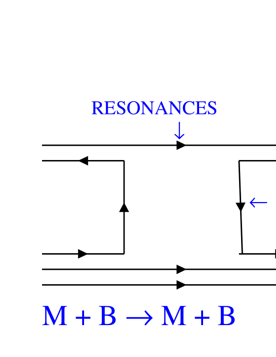
   Figure 4: Quark diagrams for meson - meson and meson - baryon scattering.

10. Shadowing Corrections ( SC ):

    To understand what is the shadowing correction ( SC ) and why we have to deal with them let us look at Fig.1 more carefully. Actually, the simple formula of Eq. (1) is correct only if the flux of “wee” partons $N$ is rather small. Better to say, that this flux is such that only one or less then one of “wee” partons has the same longitudinal and transverse momenta. However, if $N\,>\,1$, several “wee” partons can interact with the target. For example, two “wee” partons interact with the target with a cross section

    $$\sigma^{(2)}\,\,\,=\,\,\,\sigma_{0}\,\times\,\kappa$$ (26)

    where $\kappa$ is the probability for the second “wee” parton to meet and interact with the target. All “wee” partons are distributed in an area in the transverse plane which is equal $\pi\,R^{2}(s)$ and $R^{2}(s)\,\rightarrow\,\alpha^{\prime}_{P}(0)\,\ln(s)$. Therefore, $\sigma^{(2)}$ is equal to

    $$\sigma^{(2)}\,\,\,=\,\,\,\sigma_{0}\,\times\,N\,\times\,\kappa\,\,\,=\,\,\,\frac{(\,\sigma^{P}_{tot}\,)^{2}}{\pi\,R^{2}(s)}\,\,\,.$$ (27)

    Now, let us ask ourselves what should be the sign for a $\sigma^{(2)}$ contributions to the total cross section. The total cross section is just the probability that an incoming particle has at least one interaction with the target. However, in Eq. (1) we overestimate the value of the total cross section since we assumed that every parton out of the total number of “wee” partons $N$ is able to interact with the target. Actually, in the case of two parton interaction, the second parton cannot interact with the target if it is just behind the first one. The probability to find the second parton just behind the first one is equal $\kappa$ which we have estimated. Therefore, instead of flux $N$ of “wee” partons in Eq. (1) we should substitute the renormalized flux, namely

    $$RENORMALIZED\,\,\,FLUX\,\,\,=$$ (28)

    $$\,\,\,N\,\times\,\left(\,1\,\,-\,\,\kappa\,\right)\,\,\,=\,\,\,N\,\times\,\left(\,1\,\,-\,\,\frac{\sigma^{P}_{tot}}{\pi\,R^{2}(s)}\,\right)\,\,.$$

    The difference between flux of “wee” partons and the renormalized flux of “wee” partons if this difference is not very large we call shadowing and/or screening corrections. In other words,

    the shadowing corrections for the Pomeron exchange is the Glauber screening for the flux of “wee” partons.

    The analogy and terminology become more clear if you notice that Eq. (28) leads to Glauber formula for the total cross section, namely,

    $$\sigma_{tot}\,\,\,=\,\,\,\sigma^{P}_{tot}\,\,\,-\,\,\,\frac{(\,\sigma^{P}_{tot}\,)^{2}}{\pi\,R^{2}(s)}\,\,\,.$$ (29)

    If $\kappa\,\,\ll\,\,1$ we can restrict ourselves to the calculation of interaction of two “wee” partons with the target. However, if $\kappa\,\,\approx\,\,1$ we face a complicated and challenging problem of calculating all SC. We are far away from any theoretical solution of this problem especially in the “soft” interaction. What we know will be briefly reviewed in this paper.

11. Saturation of the parton ( gluon ) density:

    Saturation of the parton (gluon ) density GLR is a hypothesis about the renormalized flux of “wee” partons in the region where flux $N$ is much large than unity. More precisely, we assume that the value of $\kappa$ reaches the unitarity maximum ( $\kappa\,=\,1$) and ceases to increase. Fig. 5 gives a picture of the parton density in a target which corresponds this hypothesis. From this picture one sees that the unitarity limit can be reached at sufficiently large virtualities $Q^{2}$ ( short distances ) in the region of applicability of pQCD. It allows us to evaluate better the flux $N$ and parameter $\kappa$.

    The expression for $\kappa$ can be written in the form

    $$\kappa\,\,=\,\,xG(x,Q^{2})\frac{\sigma(GG)}{\pi R^{2}}\,\,=\,\,\frac{3\,\pi\,\alpha_{S}}{Q^{2}\,R^{2}}\,\,xG(x,Q^{2})\,\,,$$ (30)

    where

    1. $xG(x,Q^{2})$   =    the number of partons ( gluons) in the parton cascade ($N$);

    2. $R^{2}$ is the radius of the area populated by gluons in a nucleon;

    3. $\sigma(GG)$ is the gluon cross section inside the parton cascade and was evaluated in Ref.MUQI .

    Actually, at present we know $xG$ and $R^{2}$ well enough LERIHC to estimate the kinematic region where the flux of “wee” partons becomes large. This is the line (see Fig.5 )

    $$\kappa(x,Q^{2})\,\,\,=\,\,\,1\,\,.$$ (31)

    We will discuss below the physics of this equation.

    

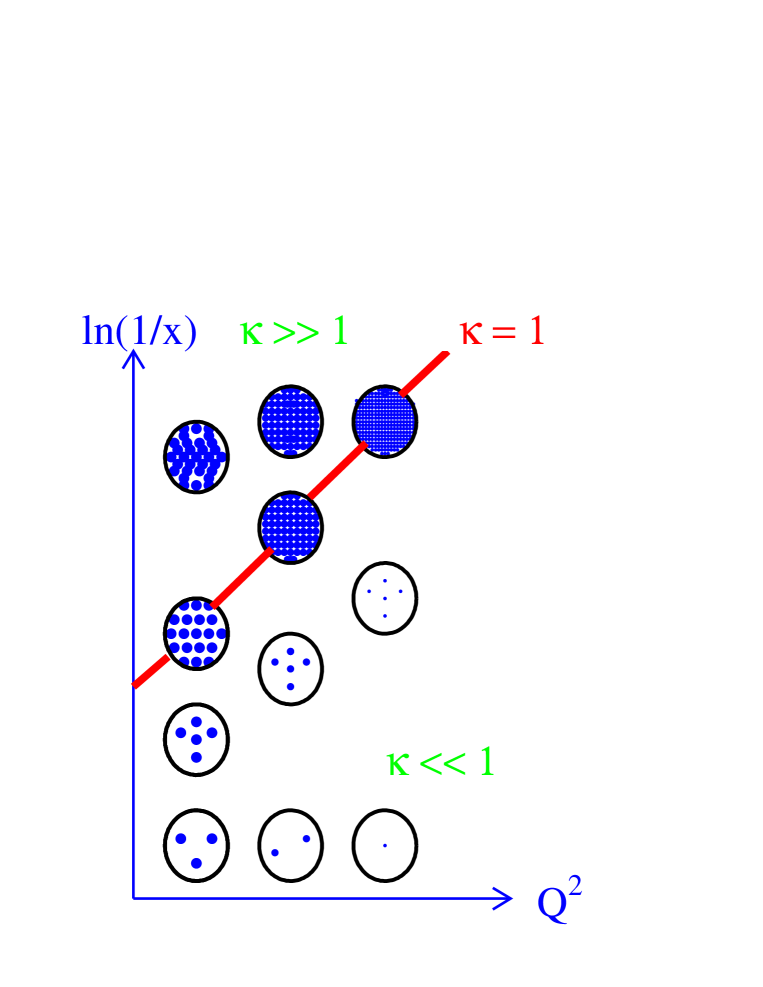
    Figure 5: Parton distributions in the transverse plane as function of $\ln(1/x)$ and $Q^{2}$.

12. Semiclassical gluon field approach:

    In the region where $N\,\,\gg\,\,1$ we can try to develop a different approach MCLER - it semiclassical gluon field approach. Indeed, due to the uncertainty relation between the number of particles and the phase of the amplitude of their production

    $$N\,\times\,\Delta\phi\,\,\geq\,\,1\,\,,$$ (32)

    we can consider $\Delta\phi\,\,\propto\,\frac{1}{N}\,\,\ll\,\,1$. Therefore, we can approach such parton system semiclassically. It means that the parton language is not more suited to discuss physics and we have to find an effective Lagrangian formulated in term of semiclassical gluonic field. A remarkable theoretical progress has been achieved in framework of such an approach MCLER but we mention this rather theoretical approach here only to illlustrate the richness of ideas that brought to the market the experiments in the deep inelastic processes mostly done at HERA and the Tevatron.

13. Impact parameter ( $\mathbf{b}_{t}$ ) representation:

    For high energy scattering it turns out to be usefull to introduce impact parameter $b_{t}$ by

    $$l\,\,\,=\,\,k\,\times\,b_{t}\,\,,$$

    where $l$ is the angular momentum in $s$ - channel of our process and $k$ is the momentum of incoming particle at high energy. High energy means that we consider the scattering process for $k\,\,a\,\,\gg\,\,1$ where $a$ is the typical size of the interaction.

    The meaning of $b_{t}$ as well as useful kinematic relations for high energy scattering is pictured in Fig.6.

    

    Figure 6: Impact parameter $b_{t}$ and useful kinematic relations for high energy scattering.

    Formally, the scattering amplitude in $b_{t}$-space is defined as

    $$a_{el}(s,b_{t})=\frac{1}{2\pi}\int d^{2}q\,\,e^{-i\vec{q_{\perp}}\cdot\vec{b}_{t}}\,\,A(s,t)$$ (33)

    where $A(s,t)$ is scattering amplitude and $t=-q^{2}_{\perp}$ is momentum transfer squared. The inverse transform for $A(s,t)$ is

    $$A(s,t)\,\,=\,\,\frac{1}{2\pi}\int a_{el}(s,b_{t})\,\,d^{2}b_{t}\,\,e^{i\vec{q}_{\perp}\cdot\vec{b_{t}}}\,\,.$$ (34)

    In this representation

    $$\sigma_{tot}=2\int d^{2}b_{t}\,\,Ima_{el}(s,b_{t})\,\,;$$ (35)

    $$\sigma_{el}=\int d^{2}b_{t}\,\,|a_{el}(s,b_{t})|^{2}\,\,.$$ (36)

14. $\mathbf{s}$ - channel unitarity:

    The most important property of the impact parameter representation is the fact that the unitarity constraint looks simple in this representation, namely, they can be written at fixed $b_{t}$.

    $$2\,Im\,a_{el}(s,b)\,\,=\,\,|a_{el}(s,b)|^{2}\,\,+\,\,G_{in}(s,b)\,\,,$$ (37)

    where $G_{in}$ is the sum of all inelastic channels. This equation is our master equation which we will use frequently during this talk.

15. A general solution to the unitarity constraint:

    Our master equation ( see Eq. (37) ) has the general solution

    $$G_{in}(s,b)\,\,=\,\,1\,\,-\,\,e^{-\,\Omega(s,b)}\,\,;$$ (38)

    $$a_{el}\,\,=\,\,i\,\{\,1\,\,-\,\,e^{-\,\frac{\Omega(s,b)}{2}\,+\,i\,\chi(s,b)}\,\}\,\,;$$

    where opacity $\Omega$ and phase $\chi=2\delta(s,b)$ are real arbitrary but real functions.

    The algebraic operations, which help to check that Eq. (36) gives the solution, are:

    $$Im\,a_{el}\,\,=\,\,1\,\,-\,\,e^{-\,\frac{\Omega}{2}}\,cos\chi\,\,;$$

    $$|a_{el}|^{2}\,\,=\,\,\left(\,1\,\,-\,\,e^{-\,\frac{\Omega}{2}\,+\,i\,\chi}\,\right)\cdot\left(\,1\,\,-\,\,e^{-\,\frac{\Omega}{2}\,-\,i\,\chi}\,\right)\,\,=\,\,1\,\,-\,\,2\,e^{-\frac{\Omega}{2}}\,cos\chi\,\,+\,\,e^{-\Omega}\,\,.$$

    The opacity $\Omega$ has a clear meaning in physics, namely $e^{-\Omega}$ is the probability to have no inelastic interactions with the target.

    One can check that Eq. (37) in the limit, when $\Omega$ is small and the inelastic processes can be neglected, describes the well known solution for the elastic scattering: phase analysis. For high energies the most reasonable assumption just opposite, namely, the real part of the elastic amplitude to be very small. It means that $\chi\,\rightarrow\,0$ and the general solution is of the form:

    $$G_{in}(s,b)\,\,=\,\,1\,\,-\,\,e^{-\,\Omega(s,b)}\,\,;$$ (39)

    $$a_{el}\,\,=\,\,i\,\{\,1\,\,-\,\,e^{-\,\frac{\Omega(s,b)}{2}}\,\}\,\,.$$

    We will use this solution to the end of this talk. At the moment, I do not want to discuss the theoretical reason why the real part should be small at high energy . I prefer to claim that this is a general feature of all experimental data at high energy.

16. The great theorems:

    Optical theorem

    The optical theorem gives us the relationship between the behaviour of the imaginary part of the scattering amplitude at zero scattering angle and the total cross section that can be measured experimentally. It follows directly from Eq. (37), after integration over $b$. Indeed,

    $$4\pi ImA(s,t=0)\,\,=\,\,\int 2Ima_{el}(s,b_{t})\,d^{2}b_{t}\,\,=$$ (40)

    $$\,\,\int\,d^{2}b_{t}\{\,|a_{el}(s,b_{t})|^{2}\,+\,G_{in}(s,b_{t})\,\,=\,\,\sigma^{el}\,+\,\sigma^{in}\,\,=\,\,\sigma_{tot}\,\,.$$

    Froissart bound

    We call the Froissart boundary the following limit of the energy growth of the total cross section:

    $$\sigma_{tot}\,\,\,\leq\,\,\,C\,\,ln^{2}s$$ (41)

    where $s$ is the total c.m. energy squared of our elastic reaction: $a(p_{a})+b(p_{b})\rightarrow a+b$, namely $s\,=\,(p_{a}\,+\,p_{b})^{2}$. The coefficient $C$ has been calculated but we do not need to know its exact value. What is really important is the fact that $C\,\propto\frac{1}{k^{2}_{t}}$, where $k_{t}$ is the minimum transverse momentum for the reaction under study. Since the minimum mass in the hadron spectrum is the pion mass the Froissart theorem predicts that $C\,\propto\,\frac{1}{m^{2}_{\pi}}$. The exact calculation gives $C\,=60mb$.

    The proofFROISSART is based on Eq. (39) and on the proven asymptotics for $\Omega$, namely,

    $$\Omega(s,b_{t})\,|_{b_{t}\,\gg\,\frac{1}{\mu}}\,\,\rightarrow\,\,s^{N}\,e^{-\,2\,\mu\,b_{t}}\,\,,$$ (42)

    where $\mu$ is the mass of the lightest hadron ( pion).

    It consists of two steps:

    1. We estimate the value of $b^{0}_{t}$ from the condition

    $$\Omega(s,b^{0}_{t})\,\,\approx\,\,1\,\,.$$ (43)

    Using Eq. (42) one contains

    $$b^{0}_{t}\,\,=\,\,\frac{N}{2\mu}\,\ln s\,\,.$$ (44)

    Note, that at high energies the value of $b^{0}_{t}$ does not depend on the exact value of $\Omega$ in Eq. (43).

    2. Eq. (35) for the total cross section we integrate over $b_{t}$ by dividing the integral into two parts $b_{t}>b^{0}_{t}$ and $b_{t}<b^{0}_{t}$. Neglecting the second part of the integral where $\Omega$ is very small yields

    $$\sigma_{tot}\,\,=\,\,4\,\pi\int^{b^{0}_{t}}_{0}\,b_{t}db_{t}\,[\,1\,\,-\,\,e^{-\frac{\Omega(s,b_{t})}{2}}\,]\,\,+\,\,4\,\pi\int^{\infty}_{b^{0}_{t}}\,b_{t}db_{t}\,[\,1\,\,-\,\,e^{-\frac{\Omega(s,b)}{2}}\,]\,\,<$$

    $$<\,\,4\pi\int^{b_{0}}_{0}bdb\,\,=\,\,2\,\pi\,b^{2}_{0}\,\,=\,\,\frac{2\pi N^{2}}{4\,\mu^{2}}\,\ln^{2}s\,\,.$$

    This is the Froissart bound.

    Pomeranchuk theorem:

    The Pomeranchuk theorem is the manifestation of the crossing symmetry, which can be formulated in the following form: one analytic function of two variables $s$ and $t$ describes the scattering amplitude of two different reactions $a+b\,\rightarrow a+b$ at $s>0$ and $t<0$ as well as $\bar{a}+b\,\rightarrow\,\bar{a}+b$ at $s<0$  $(\,u=(p_{\bar{a}}+p_{b})^{2}>0\,)$ and $t<0$.

    The Pomeranchuk theorem says that the total cross sections of the above two reactions should be equal to each other at high energy

    $$\sigma_{tot}(a\,+\,b)\,\,=\,\,\sigma_{tot}(\bar{a}\,+\,b)\,\,\,\,at\,\,\,\,s\,\rightarrow\,\,\infty\,\,,$$ (45)

    if the real part of the amplitude is smaller than imaginary part.

17. The “ black” disc approach:

    The rough realization of what we expect in the Froissart limit at ultra high energies is so called “black disc” model, in which we assume that

    $$\Omega\,\,=\,\,\infty\,\,\,\,at\,\,\,\,b\,\,<\,\,R(s)\,\,;$$

    $$\Omega\,\,=\,\,0\,\,\,\,at\,\,\,\,b\,\,>\,\,R(s)\,\,.$$

    The radius $R$ can be a function of energy and it can rise as $R\,\,\approx\,\,\ln s$ due to the Froissart theorem.

    It is easy to see that the general solution of the unitarity constraints simplifies to

    $$a(s,b)_{el}\,\,=\,\,i\,\Theta(\,R\,-\,b\,)\,\,;$$

    $$G_{in}(s,b)\,\,=\,\,\Theta(\,R\,-\,b\,)\,\,;$$

    which leads to

    $$\sigma_{in}\,\,=\,\,\int d^{2}bG_{in}\,\,=\,\,\pi\,R^{2}\,\,;$$ (46)

    $$\sigma_{el}\,\,=\,\,\int d^{2}b\,|a_{el}|^{2}\,\,=\,\,\pi\,R^{2}\,\,;$$ (47)

    $$\sigma_{tot}\,\,=\,\,\sigma_{el}\,\,+\,\,\sigma_{in}\,\,=\,\,2\,\pi\,R^{2}\,\,;$$ (48)

    $$A(s,t)\,\,=\,\,\frac{i}{2\pi}\,\int\,\,d^{2}b\Theta(\,R\,-\,b\,)\,e^{i\vec{q_{t}}\cdot\vec{b}}\,\,=\,\,i\int^{R}_{0}bdbJ_{0}(bq_{t})\,\,=\,\,i\frac{R}{q_{t}}\,J_{1}(q_{t}R)\,\,;$$

    $$\frac{d\sigma}{dt}\,\,=\,\,\pi|A|^{2}\,=\,\pi\frac{J^{2}_{1}(R\sqrt{|t|})}{|t|}\,\,.$$ (49)

    Comparison with the experimental data of the “black disc” model shows that this rather cruel model predicts all qualitative features of the experimental data such as the value of the total cross section and the minimum at certain value of $t$, furthermore the errors in the numerical evaluation is only 200 - 300%. This model certainly is not good but it is not so bad as it could be.

    Actually, this model as well as the Pomeron approach is the first model that we use to understand the new experimental data at high energy.

18. Generalized VDM for photon interaction:

    Gribov was the first one to observe GRIBOVPH that a photon ( even virtual one) fluctuates into a hadron system with life time ( coherence length ) $\tau\,\,=\,\,l_{c}\,\,=\,\,\frac{1}{mx_{B}}$ where $x_{B}=\frac{Q^{2}}{s}$, $Q^{2}$ is the photon virtuality and $m$ is the mass of the target. This life time is much larger at high energy than the size of the target and therefore, we can consider the photon - proton interaction as a processes which proceeds in two stages ( see Fig.7):

    1. Transition $\gamma^{*}\,\rightarrow\,hadrons$ which is not affected by the target and, therefore, looks similar to electron - positron annihilation;

    2. $hadron\,\,-\,\,target$ interaction, which can be treated as standard hadron - hadron interaction, for example, in the Pomeron ( Reggeon ) exchange approach .

    

    Figure 7: Two stages of photon - hadron interaction at high energy.

    These two separate stages of the photon - hadron interaction allow us to use a dispersion relation with respect to the masses $M$ and $M^{\prime}$ GRIBOVPH to describe the photon - hadron interaction ( see Fig.8 for notations ), as the correlation length $l_{c}=\frac{1}{mx}\,\gg\,R_{N}$, the target size. Based on this idea we can write a general formula for the photon - hadron interaction,

    $$\sigma(\gamma^{*}N)\,\,=\,\,\frac{\alpha_{em}}{3\,\pi}\,\int\frac{\Gamma(M^{2})\,\,d\,M^{2}}{\,Q^{2}\,+\,M^{2}\,}\,\,\sigma(M^{2},M^{\prime 2},s)\,\,\frac{\Gamma(M^{\prime 2})\,\,d\,M^{\prime 2}}{\,Q^{2}\,+\,M^{\prime 2}\,}\,\,.$$ (50)

    where $\Gamma^{2}(M^{2})=R(M^{2})$ (see Eq. (52) ) and $\sigma(M^{2},M^{\prime 2},s)$ is proportional to the imaginary part of the forward amplitude for $V\,+\,p\,\rightarrow\,V^{\prime}\,+\,p$ where $V$ and $V^{\prime}$ are the vector states with masses $M$ and $M^{\prime}$. For the case of the diagonal transition ( $M=M^{\prime}$) $\sigma(M^{2},s)$ is the total cross section for $V-p$ interaction. Experimentally, it is known that a diagonal coupling of the Pomeron is stronger than an off-diagonal coupling. Therefore, in first approximation we can neglect the off-diagonal transition and substitute in Eq. (50) $\sigma(M^{2},M^{\prime 2},s)\,=\,\sigma)M^{2}.s)\,M^{2}\,\,\delta(\,M^{2}\,-\,M^{\prime 2})$.

    

    Figure 8: The generalized Gribov’s formula for DIS.

    The resulting photon - nucleon cross section can be written written as:

    $$\sigma(\gamma^{*}N)\,\,=\,\,\frac{\alpha_{em}}{3\,\pi}\,\int\frac{R(M^{2})\,M^{2}\,d\,M^{2}}{(\,Q^{2}\,+\,M^{2}\,)^{2}}\,\sigma_{M^{2}N}(s)\,\,,$$ (51)

    where $R(M^{2})$ is defined as the ratio

    $$R(M^{2})\,\,=\,\,\frac{\sigma(e^{+}e^{-}\,\rightarrow\,hadrons)}{\sigma(e^{+}e^{-}\,\rightarrow\,\mu^{+}\mu^{-})}\,\,.$$ (52)

    The notation is illustrated in Fig.8 where $M^{2}$ is the mass squared of the hadronic system, $\Gamma^{2}(M^{2})\,=\,R(M^{2})$ and $\sigma_{M^{2}N}(s)$ is the cross section for the hadronic system to scatter off the nucleonic target.

    Experimentally, $R(M^{2})$ can be described in a two component picture: the contribution of resonances such as $\rho,\omega,\phi$,J/$\Psi$, $\Psi^{\prime}$ and so on and the contributions from quarks which give a more or less constant term changes abruptly with every new open quark - antiquark channel, $R(M^{2})\,\approx\,3\,\sum_{q}\,e^{2}_{q}$, where $e_{q}$ is the charge of the quark and the summation is done over all active quark team.

    If we take into account only the contribution of the $\rho$ - meson, $\omega$ - meson , $\phi$ and J/$\Psi$ resonances in $R(M^{2})$ we obtain the so called vector dominance model ( VDM) JJS which gives for the total cross section the following formula:

    $$\sigma_{tot}(\gamma^{*}\,+\,p\,)\,\,=\,\,\frac{\alpha_{em}}{3\pi}\,\,\sigma_{tot}(\rho+p)\sum_{i}\,\,R(M^{2}=m^{2}_{V_{i}})\{\,\frac{m^{2}_{V_{i}}}{Q^{2}\,\,+\,\,m^{2}_{V_{i}}}\,\}^{2}\,\,$$ (53)

    where $m_{V_{i}}$ is the mass of vector meson, $Q^{2}$ is the value of the photon virtuality and $R(M^{2}=m^{2}_{V_{i}})$ is the value of the $R$ in the

    mass of the vector meson which can be rewritten through the ratio of the electron - positron decay width to the total width of the resonance. Of course, the summation in Eq. (53) can be extended to all vector resonances SS or even we can return to a general approach of Eq. (50) and write a model for the off-diagonal transition between the vector meson resonances with different masses SH . We have two problems with all generalization of the VDM: (i) a number of unknown experimentally values such as masses and electromagnetic width of the vector resonances with higher masses than those that have been included in VDM and (ii) a lack of theoretical constraints on all mentioned observables. These two reasons give so much freedom in fitting of the experimental data on photon - hadron interaction that it becomes uninteresting and non - instructive. One can see from Eq. (53), that if $Q^{2}\,\gg\,m^{2}_{V}$ VDM predicts a $\frac{1}{Q^{4}}$ behaviour of the total cross section. Such a behaviour is in clear contradiction with the experimental data which show an approximate $\frac{1}{Q^{2}}$ dependence at large values of $Q^{2}$ ( i.e. scaling ).

    The solution of this puzzle as well as the systematic description of the photon - proton interaction can be reached on the basis of Gribov formula but developing a general description both “soft” and “hard” processes. The first and oversimplified version of such description was suggested by Bodelek and KwiecinskiBK and more elaborated approaches have been recently developed by Gotsman, Levin and Maor GLMPH and Martin, Ryskin and Stasto MRSPH .

19. Difftraction dissociation:

    The experimental definition of the diffractive dissociation processes:

    Diffractive dissociation processes are processes of production one ( single diffraction (SD)) or two groups of hadrons ( double diffraction ( DD ) ) with masses ( $\mathbf{M}_{1}$ and $\mathbf{M}_{2}$ in Fig.9 ) much less than the total energy ( $\mathbf{M}_{1}\,\ll\,s$ and $\mathbf{M}_{2}\,\ll\,s$ ).

    In diffractive processes no hadrons are produced in the central region of rapidity as it shown in Fig.8. This is the reason why diffractive dissociation is the simplest process with large rapidity gap ( LRG ).

    

    Figure 9-a: Lego - plot for double diffractive dissociation.

    The above definition of diffractive processes is the practical and/or experimental one. From theoretical point of view as was suggested by Feinberg FEIN and Good and Walker GW diffractive dissociation is a typical quantum mechanical process which stems from the fact that the hadron states are not diagonal with respect to the strong interaction. Let us consider this point in more details, denoting the wave functions which are diagonal with respect to the strong interaction by $\Psi_{n}$. Therefore, the amplitude of high energy interaction is equal to

    $$A_{n}\,\,=\,\,<\Psi_{n}|T|\Psi_{n^{\prime}}>\,\,=\,\,A_{n}\,\delta_{n,n^{\prime}}\,\,,$$ (54)

    where brackets denote all needed integration and $T$ is the scattering matrix. The wave function of a hadron is equal to

    $$\Psi_{hadron}\,\,\,=\,\,\,\sum^{\infty}_{n=1}\,C_{n}\Psi_{n}\,\,.$$ (55)

    Therefore, after collision the scattering matrix $T$ will give you a new wave function, namely

    $$\Psi_{final}\,\,\,=\,\,\,\sum^{\infty}_{n=1}\,\sum^{\infty}_{n^{\prime}=1}\,C_{n}<\Psi_{n}|T|\Psi_{n^{\prime}}>\Psi_{n^{\prime}}\,\,=\,\,\sum^{\infty}_{n=1}\,C_{n}\,A_{n}\,\Psi_{n}\,\,.$$ (56)

    One can see that Eq. (56) leads to elastic amplitude

    $$a_{el}\,\,=\,\,<\Psi_{final}|\Psi_{hadron}>\,\,=\,\,\sum^{\infty}_{n=1}\,\,C^{2}_{n}\,A_{n}\,\,,$$ (57)

    and to another process, namely, to production of other hadron state since $\Psi_{final}\,\,\not\equiv\,\,\Psi_{hadron}$. This process we call diffractive dissociation. The total cross section of such diffractive process we can find from Eq. (56) and it is equal to

    $$\sigma^{SD}(s,b_{t})\,\,=\,\,\sum_{final}<\Psi_{final}|\Psi_{hadron}>^{2}\,\,-\,\,<\Psi_{hadron}|\Psi_{hadron}>^{2}\,\,=$$ (58)

    $$\,\,\sum^{\infty}_{n=1}\,C^{2}_{n}\,A^{2}_{n}(s,b_{t})\,\,-\,\,\left(\,\sum^{\infty}_{n=1}\,\,C^{2}_{n}\,A_{n}(s,b_{t})\,\right)^{2}\,\,,$$

    where we regenerate our usual variable: energy ($s$) and impact parameter ( $b_{t}$ ). Using the normalization condition for the hadron wave function ( $\sum_{n}\,C^{2}_{n}\,\,=\,\,1$ ) we can see that Eq. (58) can be reduced to the form GW PUM

    $$\sigma^{SD}(s,b_{t})\,\,=\,\,<|\sigma^{2}(s,b_{t})|>\,\,-\,\,<|\sigma(s,b_{t})|>^{2}\,\,,$$ (59)

    where $<|f|>\,\,\equiv\,\,\sum_{n}C^{2}_{n}f_{n}$.

    Eq. (59) has clear optical analogy which clarify the physics of diffraction, namely, the single- slit diffraction of “white” light. Indeed, everybody knows that in the central point all rays with different wave lengths arrive with the same phase and they give a “white ” maximum. This maximum is our elastic scattering. However, the conditions of all other maxima on the screen with displacement $a$, depend on the wave lengths ( $asin\theta\,=\,k\,\lambda$ ). All of them are different from the central one and they have different colours. Sum of all these maxima gives the cross section of the diffractive dissociation.

20. Pumplin bound for SD:

    The Pumplin bound PUM follows directly from unitarity constrain of Eq. (37) which we can write for each state $n$ with wave function $\Psi_{n}$ separately:

    $$2\,\,ImA^{el}_{n}(s,b_{t})\,\,=\,\,|A^{el}_{n}(s,b_{t})|^{2}\,\,+\,\,G^{in}_{n}(s,b_{t})\,\,.$$ (60)

    Assuming that the amplitude at high energy is predominantly imagine, we obtain, as has been discussed, that

    $$|A^{el}_{n}(s,b_{t})|^{2}\,\,\leq\,\,\,G^{in}_{n}(s,b_{t}\,\,\leq\,\,\sigma^{tot}_{n}(s,b_{t})\,\,.$$ (61)

    After summing over all $n$ with weight $C^{2}_{n}$ ( averaging ) one obtains the Pumplin bound:

    $$\sigma_{el}(s,b_{t})\,\,+\,\,s^{SD}(s,b_{t})\,\,\leq\,\sigma_{tot}(s,b_{t})\,\,,$$ (62)

    where $\sigma_{el}(s.b_{t})\,\,=\,\,|a_{el}(s,b_{t})|^{2}$, $\sigma_{tot}(s,b_{t})\,\,=\,\,2\,Im\,a_{el}(s,b_{t})$ and $s^{SD}(s,b_{t})\,\,=\,\,\sum_{M}|a_{M}(s,b_{t})|^{2}$ .

21. Unitarity limit of SD for hadron and photon induced reactions:

    At high energy $A^{el}_{n}\,\,\Longrightarrow\,\,1$ ( see Eq. (41) ). It means that at high energy the scattering matrix does not depend on $n$. Therefore from Eq. (56) one can derive

    $$\Psi_{final}\,\,\,=$$ (63)

    $$\,\sum^{\infty}_{n=1}\,\sum^{\infty}_{n^{\prime}=1}\,C_{n}<\Psi_{n}|T|\Psi_{n^{\prime}}>\,\,\Psi_{n^{\prime}}\,\,=\,\,\sum^{\infty}_{n=1}\,C_{n}\,\Psi_{n}\,\,\,\equiv\,\,\Psi_{hadron}\,\,.$$

    Eq. (63) says that $\sigma^{SD}\,\,\Longrightarrow\,\,0$ at high energies. Performing integration over $b_{t}$ it is easy to obtain that in the hadron induced reactions

    $$\frac{\sigma^{SD}}{\sigma_{el}}\,\,\,\propto\,\,\frac{1}{\ln s}\,\,\Longrightarrow\,\,0.$$ (64)

    It should be stressed, that we should be careful with this statement for photon ( real or virtual ) induced reactions. As we have seen, in Gribov formula we have an integration over mass. For each mass we have the same property of the diffractive dissociation as has been presented in Eq. (64). However, due to integration over mass in Eq. (51)the ratio of the total diffractive dissociation process to the total cross section is equal to

    $$\frac{\sigma^{DD}_{tot}(\gamma^{*}p\,\rightarrow\,M+p)}{\sigma_{tot}(\gamma^{*}p\,\rightarrow\,\gamma^{*}+p)}\,\,\,\Longrightarrow\,\,\,\frac{1}{2}\,\,.$$ (65)

22. Survival Probability of Large Rapidity Gaps:

    We call any process a large rapidity gap ( LRG )process if in a sufficiently large rapidity region no hadrons are produced. Historically, both Dokshitzer et al. KHOZE and Bjorken BJLRG , suggested LRG as a signature for Higgs production in W-W fusion process in hadron-hadron collisions. The definition of the survival probability ( $<S^{2}>$ ) is clear from Fig. 9-b. Indeed, let us consider the typical LRG process - production of two jets with large transverse momenta $\vec{p}_{t1}\,\approx\,-\,\vec{p}_{t2}\,\,\gg\,\,\mu$ , where $\mu$ is the typical mass scale of “soft” processes , and with LRG between these two jets. Therefore, we consider the reaction:

    $$p(1)\,\,+\,\,p(2)\,\,\longrightarrow M_{1}[hadrons\,\,+\,\,jet_{1}(y_{1},p_{t1})]$$ (66)

    $$+\,\,LRG[\Delta y=|y_{1}-y_{2}|]\,\,+\,\,M_{2}[hadrons\,\,+\,\,jet_{2}(y_{2},p_{t2})]\,\,,$$

    where $y_{1}$ and $y_{2}$ are rapidity of jets and LRG $\Delta y=|y_{1}-y_{2}|\,\,\gg\,\,1$. To produce two jets with LRG between them we have two possibility:

    1. This LRG appears as a fluctuation in the typical inelastic event. However, the probability of such a fluctuation is proportional to $e^{-\frac{\Delta y}{L}}$ and the value of the correlation length $L$ we can evaluate $L\,\approx\,\frac{1}{\frac{dn}{dy}}$, where $\frac{dn}{dy}$ is the number of particles per unit in rapidity. Therefore, LRG means that $\Delta y\,\gg\,L$  ;

    2. The exchange of colourless gluonic state in QCD is responsible for the LRG. This exchange we denote as a Pomeron in Fig.9-b. The ratio the cross section due to the Pomeron exchange to the typical inelastic event generated by the gluon exchange ( see Fig. 9-b ) we denote $F_{s}$. Using the simple QCD model for the Pomeron exchange, namely, the Low-Nussinov LN idea that the Pomeron = two gluon exchange, Bjorken gave the first estimate for $F_{s}\,\approx\,\,0.15\%$. This is an interesting problem to obtain a more consistent theoretical estimates for $F_{s}$, but $F_{s}$ is not the survival probability. $F_{s}$ is the probability of the LRG process in a single parton shower.

    However, each parton in the parton cascade of a fast hadron could create its own parton chain which could interact with one of the parton of the target. Therefore, we expect a large contribution of inelastic processes which can fill the LRG. To take this multi shower interaction we introduce the survival probability $<S^{2}>$ ( see Fig.9-b ).

    To calculate $<S^{2}>$ we need to find the probability that all partons with rapidity $y_{i}\,>\,y_{1}$ in the first hadron ( see Eq. (66) and partons with $y_{j}\,<\,y_{2}$ in the second hadron do not interact inelastically and, therefore, they cannot produce hadrons in the LRG. As we have discuss, the meaning of Eq. (41) in physics is that

    $$P(y_{i}-y_{j},b^{ij}_{t})\,\,=\,\,e^{-\,\,\Omega(y_{i}-y_{j},b^{ij}_{t})}$$ (67)

    gives you the probability that two partons with rapidities $y_{i}$ and $y_{j}$ and with $b^{ij}_{t}\,\,=\,\,|\vec{b}_{t,i}\,-\,\vec{b}_{t,j}|$ do not interact inelastically.

    The general formula for $<S^{2}>$ reads

    $$<S^{2}>\,\,\,=\,\,\frac{\int\,dy_{i}\,dy_{j}\,d^{2}b^{ij}_{t}\,\,P_{1}(y_{i},y_{1},b_{t,i})\,P_{2}(y_{j},y_{2},b_{t,j})\,\,P(y_{i}-y_{j},b^{ij}_{t})}{\int\,dy_{i}\,dy_{j}\,d^{2}b^{ij}_{t}\,\,P_{1}(y_{i},y_{1})\,P_{2}(y_{j},y_{2})}\,\,,$$ (68)

    where $P_{1}(y_{i},y_{1})(P_{2}(y_{j},y_{2})$ is probability to find two partons with rapidity $y_{1}$ and $y_{i}$ ( $y_{2}$ and $y_{j}$ ) in hadron $1$ ( $2$ ), respectively. The deep inelastic structure function is $x_{1}G(x_{1},p^{2}_{t,1})\,\,=\,\,\int dy_{i}\,d^{2}b_{t,i}\,\,P_{1}(y_{1}=\ln(1/x_{1}),y_{i},b_{t,i})$.

    Unfortunately, there is no calculation using a general formula of Eq. (68). What we have on the market is the oversimplified calculation in the Eikonal model ( see Ref. GOTSMAN ) in which we assume that only the fastest partons from both hadrons can interact.

    

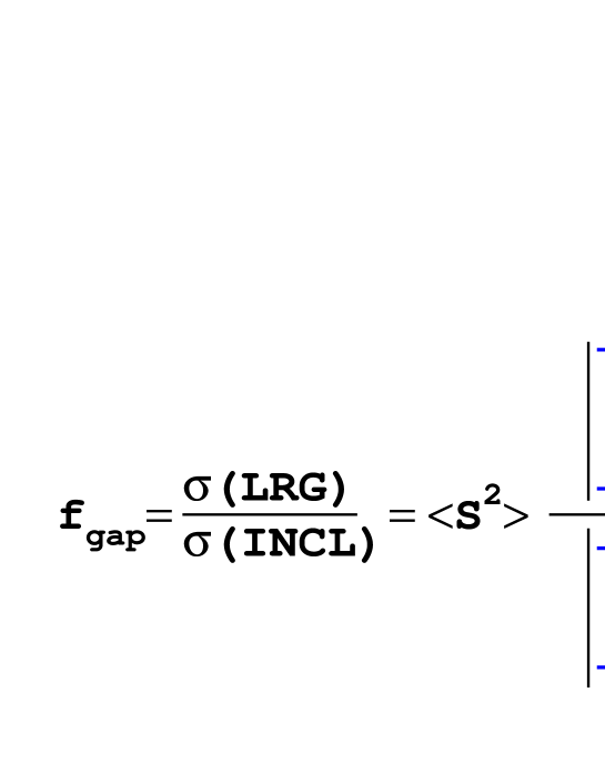
    Figure 9-b: Typical LRG process .

I “S O F T”    P O M E R O N:

II “Theorems” about Pomeron

In this section we collect main properties of the “soft” Pomeron which we have discussed in the previous section.

• There is only one Pomeron.

  It means that only “soft” Pomeron has a chance to be a simple Regge pole (Reggeon) ( see previous section for details).

• The Pomeron is the Reggeon with $\mathbf{\Delta}_{P}(0)\,=\,\alpha_{P}(0)-1\,\ll\,1$

  Being a Reggeon, the Pomeron has all typical features of a Reggeon written in Eq. (9) and presented in Fig. 10. They are:

  

  Figure 10: The exchange of the Pomeron.

  $\star$ Analiticity  ;

  $\star$ Resonances  ;

  $\star$ Factorization  ;

  $\star$ Definite phase  ;

  $\star$ Increase of the radius of interaction  ;

  $\star$ Shrinkage of the diffraction peak  ;

  Increase of the radius of interaction:

  Eq. (9) can be rewritten in the impact parameter representation taking the integral of Eq. (33) as follows

  $$a_{el}(s,b_{t})\,=\,g_{1}(0)\,g_{2}(0)(s/s_{0})^{\Delta_{P}}\frac{1}{\pi R^{2}(s)}e^{-\frac{b^{2}_{t}}{R^{2}(s)}}$$ (69)

  with

  $$R^{2}(s)\,=\,R^{2}_{0}\,+\,4\,\alpha^{\prime}_{P}\,\ln(s/s_{0})$$

  One can see, that the typical impact parameters turns out to be of the order of $R(s)$. This fact means that the radius of interaction increases with energy.

  Shrinkage of the diffraction peak:

  Using Eq. (9) we can see that the $t$-dependence is determined mostly by the Pomeron exchange since

  $$\frac{\frac{d\sigma}{dt}}{\frac{d\sigma}{dt}\,|_{t=0}}\,\propto\,e^{-\,2\alpha^{\prime}_{P}\,\ln(s/s_{0})\,|t|}\,\,.$$ (70)

  Therefore, the differential cross section falls down rapidly for $|t|\,\,\geq\,\,\frac{1}{\alpha^{\prime}_{P}(0)\,\ln(s/s_{0})}$. This phenomena we call the shrinkage of the diffraction peak. It should be stressed that this shrinkage has been observed in many “soft” reactions, but it seems to me that the value of $\alpha^{\prime}_{P}(0)$ has not been determined yet from the experimental data.

• Pomeron  =  gluedynamics at high energy .

  There is no resonances on the Pomeron trajectory. This is the principle difference between the secondary Reggeons and the Pomeron. In duality approach the Pomeron does not appear in dual diagrams of the first order and

  $$P\,\,\propto\,\,\frac{\alpha_{S}}{N_{c}}\,(\,\frac{s}{s_{0}}\,)^{C\alpha_{S}}\,\,.$$

  The common believe, which is based on the experience with duality approach and QCD calculations, is that

  The Pomeron $\longrightarrow$ glueballs $\longrightarrow$ gluon interaction at high energy.

• There is no arguments for a Pomeron but it describes experimental data quite well

  

  Figure 11: The total cross section in the Pomeron approach in the Donnachie - Landshoff approach ( full line ) and in the Eikonal model (dotted line)

  Fig.11 shows that the Pomeron exchange is able to describe the experimental data on total proton - proton scattering at high energy. Of course, this is an example. More systematic description of the data one can find in Ref.TABLE or/and in original Donnachie - Landshoff papers DL .

• Pomeron is a “ladder” diagram for a superconvergent theory like $\mathbf{g}\phi^{3}$.

  The charm of the Pomeron approach is in the relation between the elastic or / and quasi - elastic reactions ( like diffractive dissociation, for example ) and the multiparticle production at high energy. The simple picture for the Pomeron exchange presented in Fig.12 was, is and, unfortunately, will be our practical tool for application of the Pomeron phenomenology to the processes of the multiparticle production.

  

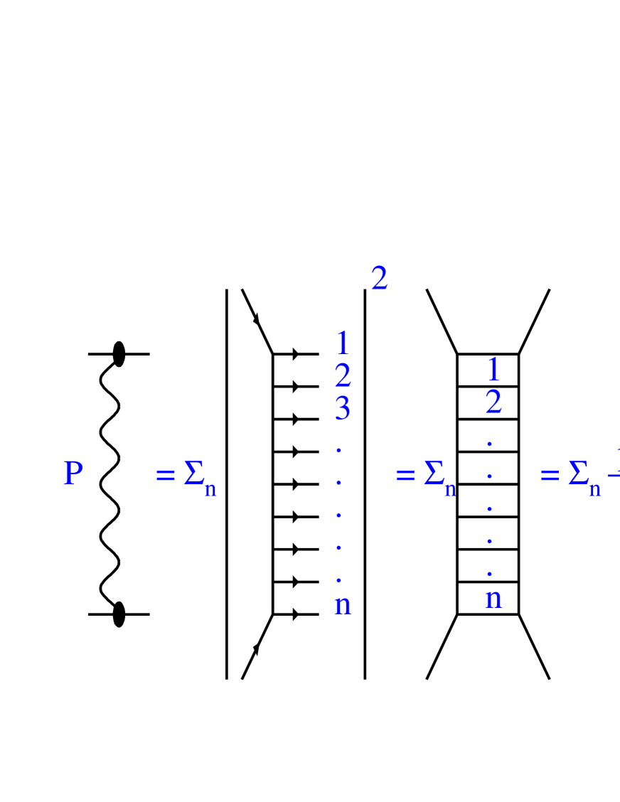
  Figure 12: The Pomeron structure in $g\phi^{3}$ - theory ( parton model ).

  In spite of the simplicity of this picture we would like to mention that it appears in simple but strict approximation, so called leading log s approximation. In this approximation we sum all contributions to Feyman diagrams of the order of $(\,\frac{g^{2}}{m^{2}}\ln s\,)^{n}$, neglecting smaller terms.

  It should be stressed that this approach reproduces the main property of observed multiparticle production at high energies.

  $\star$ Power - like behaviour of the total cross section

  $$\sigma_{tot}\,\propto\,(\frac{s}{s_{0}})^{\Sigma(q^{2})}\,\,;$$

  $\star$ Pomeron = only multiparticle production with $<N>\,\propto\,\ln s$  ;

  $\star$ Uniform rapidity distribution of the produced particles  ;

  

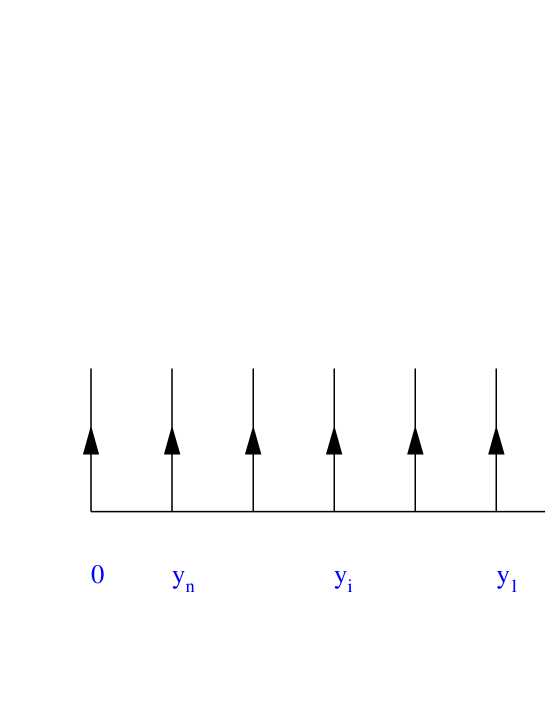
  Figure 13: Uniform distribution in rapidity in $g\phi^{3}$ - theory ( parton model ) .

  $\star$ Average transverse momentum of produced particles does not depend on energy  ;

  $\star$ There are no correlation between produced particles  ;

  $\star$ Poisson multiplicity distribution  ;

  $\star$ Increase of the interaction radius due to the random walk in impact parameters  ;

  

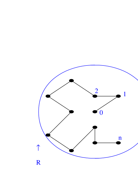
  Figure 14: Random walk in the transverse plane in $g\phi^{3}$ - theory ( parton model ).

The increase of the interaction radius is seen in Fig.14 and follows directly from uncertainty relation and from the fact that the mean transverse momentum of particles ( partons ) does not depend on energy. Indeed, from uncertainty principle:

$$\Delta\,b_{t}\,\times\,<k_{t}>\,\,\approx\,\,1\,\,,$$ (71)

where $<k_{t}>$ is the mean parton momentum. Therefore, each emission changes the position of the parton in impact parameter space on the value $\Delta b_{t}\,\,\approx\,\,\frac{1}{<k_{t}>}$. After $n$ emission the parton will be on the distance $<b^{2}_{t,n}>\,\,\propto\,\frac{1}{<k_{t}>}\,n$. Since the average number of emission $N\,\,\propto\,\,\ln s$, the radius of interaction

$$R^{2}(s)\,\,=\,\,<b^{2}_{t,N}>\,\,\propto\,\,\frac{1}{<k_{t}>}\,N\,\,=\,\,\frac{1}{<k_{t}>}\,\ln s\,\,.$$ (72)

III Donnachie - Landshoff Pomeron

In practice, when we say “soft” Pomeron, we mean so called Donnachie - Landshoff Pomeron. Donnachie and Landshoff suggested the simplest picture of high energy interaction - the exchange of the Pomeron which is a Regge pole. Note, that the Donnachie - Landshoff approach to high energy scattering is more complicated than the exchange of the Pomeron. They also included a week shadowing corrections as we will discuss below. I want to stipulate that in this section I discuss only the D-L Pomeron but not the D-L approach. In their simple picture Donnachie and Landshoff gave the most economic and elegant description of the experimental data mostly related to the total and elastic cross sections. From fitting procedure they found that the D-L Pomeron has the following features:

1.    The Pomeron intercept, $\Delta\,\,=\,\,\alpha_{P}(0)\,-\,1\,\,=\,\,0.08$  ;

2.    The Pomeron slope $\alpha^{\prime}_{P}(0)\,\,=\,\,0.25\,GeV^{-2}$  ;

3.    The linear parameterization for the Pomeron trajectory $\alpha_{P}(t)\,\,=\,\,\alpha_{P}(0)\,\,+\,\,\alpha^{\prime}_{P}(0)\,\,t$ can be used to fit the experimental data  ;

4.   The additive quark model ( AQM ) can be used to to find the $t$ - dependence of the Pomeron - hadron vertices. In AQM the Pomeron vertex is proportional to the electromagnetic form factor of the hadron.

IV Seven arguments against D - L Pomeron

In spite of the wide use of the D-L Pomeron or, may be, because of this, the D-L Pomeron is seriously sick. Here, we want to list seven arguments against the D-L Pomeron which, we think, show that D-L Pomeron ( and D-L approach, which we will discuss below) is close to its last days of existence. In what follows we try to separate the D-L Pomeron from D-L approach which includes not only the Pomeron but also week SC.

1. The D-L Pomeron violates unitarity (   $\mathbf{a}_{el}(s,b_{t})\,\leq\,1$ just around the corner   )  ;

   

   Figure 15: $a_{el}$ for the D-L Pomeron .

   From Fig.15 one can see that at $\sqrt{s}\,\approx\,\,3000GeV$ the D-L Pomeron violates the $s$-channel unitarity constrain ( see Eq. (37) ). The success of the description of the experimental data on total and elastic cross section is mostly due to the fact that the area, in which $a_{el}(s,b_{t})\,>\,1$ in Fig. 15, is much smaller than the total area. However, the fact that $a_{el}$ is close to unity should reveal itself in the description of other processes which are more sensitive to the value of $a_{el}$.

2. The D-L Pomeron gives $\mathbf{G}_{in}(s,b_{t})$ which is quite different from the Pomeron one   ;

   

   Figure 16: $G_{in}$ for the D-L Pomeron .

   In Fig. 16 we plot the value of $G_{in}(s,b_{t})$ which we calculated from the $s$-channel unitarity constrain of Eq. (37), namely,

   $$G_{in}(s,b_{t})\,\,=\,\,2\,Im\,a_{el}(s,b_{t})\,\,-\,\,|a_{el}(s.b_{t})|^{2}\,\,,$$

   using the D-L parameterization for $a_{el}(s,b_{t})$. One can see that $G_{in}$ turns out to be very close to unity in accessible energy range. Comparing $b_{t}$-dependence of $a_{el}(s,b_{t})$ ( see Fig.14 ) and $G_{in}(s,b_{t})$ ( see Fig.15) one can see that this dependence is quite different for them. It means that the main idea of the parton model (see Fig.1) that the exchange of the Pomeron is closely related to the multiparticle ( multiparton ) production is broken in the D-L approach. In other words, the most charming feature of the Pomeron approach as a whole, namely, the ability of the Pomeron to describe both elastic and inelastic processes, turns out to be inconsistent in the D-L approach. For me, it is too high price for the fit of the elastic and total cross sections even if it is a simple one.

3. The D-L Pomeron and D-L approach cannot describe the $\mathbf{s}$-dependence of the diffractive dissociation cross section, measured at CDF  ;

   

   Figure 17: $\frac{\sigma_{el}}{\sigma_{tot}}$ and $\frac{\sigma^{SD}}{\sigma_{tot}}$ versus $\ln(s/s_{0})$ with $s_{0}=400GeV^{2}$.

   For D-L Pomeron $\sigma^{SD}\,\,\propto\,\,(\,\frac{s}{s_{0}}\,)^{2\Delta_{P}}$ while $\sigma_{tot}\,\,\propto\,\,(\,\frac{s}{s_{0}}\,)^{\Delta_{P}}$. Therefore, for the D-L Pomeron

   $$\frac{s^{SD}}{\sigma_{tot}}\,\,\,\propto\,\,\,(\,\frac{s}{s_{0}}\,)^{\Delta_{P}}\,\,,$$ (73)

   while experimentally CDFSD the energy dependence of this ratio is quite different as Fig.17 demonstrates. Week SC of the D-L approach cannot change this conclusion. It turns out that SC should be as strong as in the Eikonal model or even stronger to describe the CDF data on SD.

4. The parameters of the D-L Pomeron do not fit data quite well  ;

   The parameters of the D-L Pomeron were mostly fitted from the scattering data but the D-L Pomeron trajectory predicts a resonance at $m^{2}\,\approx\,\,4\,GeV^{2}$ with spin 2 which was not found experimentally. On the other hand, the experimental data. especially new HERA data on photon - proton scattering show that the shrinkage of the diffraction peak ( $\alpha^{\prime}_{P}(0)$ ) is different for different particles HERASHR .

5. The D-L Pomeron and /or D-L Approach cannot describe the CDF data on double parton cross section  ;

   We will comment on this below after discussion of the shadowing corrections. We will show that the double parton cross section is closely related to the collision of the two parton showers which are absent in the D-L Pomeron and too small in the D-L approach.

6. The D-L Pomeron and /or D-L Approach predicts Survival Probability for LRG processes $\rightarrow$ 1 and, therefore, cannot describe the measured LRG processes at the Tevatron   ;

   As we have discussed in section 1 the origin of the survival probability is the fact that there are many parton shower interactions with the target. If we have only the exchange of the Pomeron or, in other words, only;y one parton shower interaction the survival probability is equal to unity. Experimentally D0LRG , this survival probability is, at least, 0.1 and it shows a substantial $s$ - dependence ( see Ref GOTSMAN for details ). In D-L approach this survival probability is close to unity since the value of the SC that they suggested is too small.

7. The D-L Pomeron and /or D-L Approach cannot reproduce the Glauber Shadowing for hadron - nucleus interactions  ;

   It is well known that the Glauber Shadowing can be described in the Reggeon approach as the multiPomeron exchange of the incoming particle with nucleons in a nucleus. In D-L approach such multiPomeron exchange is suppressed. On the contrary for nucleus - nucleus interaction D-L approach gives the Glauber formula since the exchange of the Pomerons between different nucleons from different nuclei are not suppressed. Therefore, in the D-L approach the Glauber shadowing for hadron - nucleus and nucleus - nucleus interactions look quite different. In the extreme case of the D-L Pomeron approach they predict that

   $$\sigma_{tot}(hadron+nucleus)\,\,\propto\,\,A$$

   while

   $$\sigma_{tot}(nucleus+nucleus)\,\,\propto\,\,A^{\frac{2}{3}}\,\,.$$

V Shadowing corrections ( SC )

In this section I discuss the shadowing ( screening, absorption ) corrections to the Pomeron exchange. Formally speaking,in the Reggeon approach such corrections can be pictured as the exchange of many Pomerons (see Figs.18a - 18b for examples). The only question, that we should answer, is how can we sum all these complicated diagrams?

Figure 18-a: The space - time picture in the parton approach for the SC induced by three Pomeron exchange .

Figure 18-b: The space - time picture in the parton model for the first “fan” Pomeron diagram .

V.1 Several general remarks:

• There is no Pomeron without SC  ;

  It means that there is no any theoretical idea why many Pomeron exchange can be equal to zero. Therefore, our main strategy in operating with the SC is to find the kinematic region in which the SC are small, to develop a technique how to calculate the SC when they are small and to built a model ( better theory of course but practically this is a problem for future) to approach SC in the kinematic region when they are large.

• SC follow from the s-channel unitarity  ;

  To understand why SC follow from the $s$-channel unitarity let us generalize the solution to the unitarity constrains of Eq. (37) using the hadronic states which are diagonal with respect to strong interaction and which have wave functions $\Psi_{n}$, as we did discussing the diffraction dissociation processes in the previous section ( see Eq. (54) - Eq. (59) ). For each of this state we have a unitarity constrain of Eq. (LABEL:PS1) and we can find a solution to Eq. (60) assuming that $Im\,A_{n}(s,b_{t})\,\,\gg\,\,Re\,A_{n}(s,b_{t})$:

  $$A^{el_{n}}\,\,\,=\,\,\,i\,\frac{1}{2}\,\{\,1\,\,\,-\,\,\,e^{-\frac{\Omega_{n}(s,b_{t})}{2}}\,\}\,\,;$$ (74)

  $$G^{in}_{n}\,\,\,\,=\,\,\,\,1\,\,\,-\,\,e^{-\Omega_{n}(s,b_{t})}\,\,.$$ (75)

  Let us assume that $\Omega_{n}\,\,\ll\,\,1$ and expand Eq. (74) and Eq. (75) with respect to $\Omega_{n}$:

  $$A^{el}_{n}(s,b_{t})\,\,=\,\,\frac{\Omega_{n}(s,b_{t})}{2}\,\,\,-\,\,\frac{\Omega^{2}_{n}(s,b_{t})}{8}\,\,\,+\,\,\,O(\Omega^{3}_{n})\,\,;$$ (76)

  $$G^{in}_{n}(s,b_{t})\,\,\,=\,\,\,\Omega_{n}(s,b_{t})\,\,\,-\,\,\,\frac{\Omega^{2}_{n}(s,b_{t})}{2}\,\,\,+\,\,\,O(\Omega^{3}_{n})\,\,.$$ (77)

  Using Eq. (55) - Eq. (58) we obtain for the observables:

  $$\sigma_{el}(s,b_{t})\,\,\,=\,\,\,\frac{1}{4}\,\,\left(\,\sum^{\infty}_{n=1}\,C^{2}_{n}\,\Omega_{n}(s,b_{t})\,\right)^{2}\,\,;$$ (78)

  $$\sigma_{tot}\,\,\,=\,\,\,\sum^{\infty}_{n=1}\,C^{2}_{n}\,\Omega_{n}(s,b_{t})\,\,\,-\,\,\,\frac{1}{4}\,\left(\,\sum^{\infty}_{n=1}\,C^{2}_{n}\,\Omega^{2}_{n}(s,b_{t})\,\right)\,\,;$$ (79)

  $$\sigma_{in}\,\,\,=\,\,\,\sum^{\infty}_{n=1}\,C^{2}_{n}\,\Omega_{n}(s,b_{t})\,\,\,-\,\,\,\frac{1}{2}\,\left(\,\sum^{\infty}_{n=1}\,C^{2}_{n}\,\Omega^{2}_{n}(s,b_{t})\,\right)\,\,;$$ (80)

  $$\sigma^{SD}\,\,\,=\,\,\,\frac{1}{4}\,\{\,\sum^{\infty}_{n=1}\,C^{2}_{n}\,\Omega^{2}_{n}(s,b_{t})\,\,\,-\,\,\,\left(\,\sum^{\infty}_{n=1}\,C^{2}_{n}\,\Omega_{n}(s,b_{t})\,\right)^{2}\,\}\,\,.$$ (81)

  As we have discussed, in the framework of converged theories or in the parton model, the one Pomeron exchange corresponds to the typical inelastic event with production of the large number of particles. Therefore, we can associate this exchange with $\Omega$ since one can see that $\sigma_{tot}(s,b_{t})\,\,=\,\,\sigma_{in}(s,b_{t})\,\,\propto\,\,\Omega$. All terms which are proportional to $\Omega^{2}$ describe the two Pomeron exchange and they induce the SC.

• The scale of SC from the experimental data on $\mathbf{\sigma}_{tot},\sigma_{el}$ and $\mathbf{\sigma}^{SD}$;

  We can evaluate the scale of the SC using experimental data on $\sigma_{tot},\sigma_{el}$ and $\sigma^{SD}$. Indeed, we can write the expression of the total cross section in the form:

  $$\sigma_{tot}\,\,\,=\,\,\sigma^{P}_{tot}\,\,\,-\,\,\,\Delta\sigma^{SC}_{tot}\,\,,$$ (82)

  where $\sigma^{P}_{tot}$ is the contribution of the Pomeron exchange to the total cross section. Summing Eq. (78) and Eq. (81) we derive that

  $$\Delta\sigma^{SC}_{tot}\,\,\,=\,\,\,\sigma_{el}\,\,+\,\,\sigma^{SD}\,\,$$ (83)

  or

  $$\kappa\,\,=\,\,\frac{\Delta\sigma_{tot}}{\sigma_{tot}}\,\,=\,\,\frac{\sigma_{el}\,+\,\sigma^{SD}}{\sigma_{tot}}\,\,\propto\,\,\frac{\int d^{2}b_{t}\,\Omega^{2}(s,b_{t})}{\int d^{2}b_{t}\,\Omega(s,b_{t})}\,\,.$$ (84)

  Fig.17 shows that in the wide range of energy $\kappa\,\,\approx\,\,0.34$ and, therefore, we can consider the single Pomeron exchange as a good approximation only with the errors of about 34%. I do not think, we need to argue that such an approximation cannot be considered as a good one.

• The scale of SC from the inclusive correlation function  ;

  It is well known ( see for example Ref.MYLEC ) that the Reggeon approach gives the two particle rapidity correlation function, which defined as:

  $$R\,\,=\,\,\frac{\frac{d^{2}\sigma(y_{1},y_{2})}{\sigma_{tot}dy_{1}dy_{2}}}{\frac{d\sigma(y_{1})}{\sigma_{tot}\,dy_{1}}\frac{d\sigma(y_{2})}{\sigma_{tot}dy_{2}}}\,\,-1$$ (85)

  where $\frac{d^{2}\sigma}{dy_{1}dy_{2}}$ is the double inclusive cross section for the reaction:

  $$a\,\,+\,\,b\,\,\rightarrow\,\,1(y_{1})\,\,+\,\,2(y_{2})\,\,+\,\,anything\,\,.$$

  The correlation function can be written in the form:

  $$R(y_{1},y_{2})\,\,=\,\,SR\,\times\,e^{-\frac{\Delta y}{L_{cor}}}\,\,\,+\,\,LR\,\,.$$ (86)

  These two terms in Eq. (86) correspond to two Reggeon diagrams in Fig.19. The first diagram gives the short range correlations which falls at $\Delta y\,=\,|y_{1}-y_{2}|\,>\,L_{cor}$ with $L_{cor}\,=\,\frac{1}{\alpha_{R}(0)}$, where $\alpha_{R}(0)$ is the intercept of the secondary Reggeon trajectory ( see Fig.2 ) and $\alpha_{R}(0)\,\approx\,0.5$. The second term is closely related to the shadowing correction to the total cross section and it is equal:

  $$LR\,\,\,=\,\,2\,\frac{\Delta\sigma_{tot}}{\sigma_{tot}}\,\,.$$ (87)

  Therefore, if we can separate the long range rapidity correlation from the short range one we will measure the value of the SC.

  

  Figure 19: The rapidity correlation function $R$ in the Reggeon approach .

  The CDF collaboration at the Tevatron did this. The CDF measured the process of inclusive production of two “hard” jets with large but almost compensating transverse momenta in each pair( $\vec{p}_{t1}\,\approx\,-\vec{p}_{t2}\,\gg\,\mu$, where $\mu$ is the scale of “soft” interactions) and with values of rapidity that are very similar. Such pairs cannot be produced by one Pomeron exchange or in other words in one parton shower collision if the difference in rapidity of these pairs is small that $1/\alpha_{S}(p^{2}_{t})$. They can only be produced in double parton shower interaction and their cross section can be calculated using the Mueller diagrams MUD given in Fig.20. It can be written in the form CDFDP

  $$\sigma_{DP}\,\,=\,\,m\,\frac{\sigma_{incl}(\,2\,\,jets\,)\,\,\sigma_{incl}(\,2\,\,jets\,)}{2\,\,\sigma_{eff}}\,\,,$$ (88)

  where factor $m$ is equal 2 for different pairs of jets and to 1 for identical pairs. The experimental value of $\sigma_{eff}\,\,=\,\,14.5\,\pm\,1.7\,\pm\,2.3\,mb$ CDFDP .

  Comparing Eq. (88) with Eq. (87) one can obtain the estimates for

  $$\frac{\Delta\sigma_{tot}}{\sigma_{tot}}\,\,=\,\,\frac{\sigma_{in}}{4\,\sigma_{eff}}\,\,\approx\,\,40-50\,\%\,\,.$$ (89)

  

  Figure 20: The Mueller ( Reggeon ) diagram for double parton interaction .

• The scale of SC from diffractive dissociation at HERA  ;

  As we have discussed the value of the SC crusially depends on the size of the target ( see Eq. (27) and Eq. (28) ) and $\kappa\,\,\propto\,\,\frac{\sigma^{P}_{tot}}{\pi\,R^{2}(s)}$. Actually, $R^{2}$ reflects the integration over $q_{t}$ ( $b_{t}$ ) in the first diagrams for the SC ( see Figs. 21 and 22 ). In some sense

  $$\int\,\,d^{2}q_{t}\,\,\,\Longrightarrow\,\,\,\frac{1}{\pi\,R^{2}}\,\,.$$

  

  Figure 21: The first order SC $\propto\,\,\int\,d^{2}b_{t}\Omega^{2}(s,b_{t})$ in the additive quark model for the proton .

  

  Figure 22: The first order SC $\propto\,\,\int\,d^{2}b_{t}\Omega^{2}(s,b_{t})$ DIS with the proton in the additive quark model for the proton .

  The HERA data on diffractive photoproduction of $J/\Psi$ meson HERAPSI give a unique possibility to find $R^{2}$. Indeed, (i) the experimental values for the slope ( see Fig.23 ) are $B_{el}\,=\,4\,GeV^{-2}$ and $B_{in}\,=\,1.66\,GeV^{-2}$ and (ii) the cross section for $J/\Psi$ diffractive production with and without proton dissociation are equal. Neglecting the $t$ dependence of the upper vertex in Fig.22, we can estimate the value of $R^{2}$. It turns out that $R^{2}\,\approx\,5\,GeV^{-2}$ or in other word it approximately in 2 times smaller than the radius of the proton. Using Eq. (27) and this value for $R^{2}$ we obtain that $\Delta\sigma/\sigma\,\approx\,\,40\%$.

V.2 Weak SC ( Donnachie - Landshoff approach ):

Let us ignore everything that I have discussed in the previous section about the size of the SC. Let us pretend that we have not learned Eq. (78) - Eq. (81) and let us try to estimate the value of the SC using only experimental data. In my opinion this was the logic of the Donnachie - Landshoff approach. Indeed, they achieved a good description of the experimental data on $\sigma_{tot}$ and $\sigma_{el}$ and, therefore, they could expect that the value of SC would be small. However, they had to introduce the SC to describe the $t$- dependence of the elastic cross section. Indeed, the experiment shows a clear structure in $t$ dependence - a minimum at $t\,\approx 1.3-1.4\,GeV^{2}$ ( see Fig.23 ). Everybody knows that such a structure is very typical for interaction in optics as well as for interaction of any waves with the target with definite size. However, the Pomeron exchange does not reproduces this typical diffractive structure. The reason for this is clear since the Pomeron corresponds to predominantly inelastic production and strictly speaking the elastic cross section should be considered as small in pure Pomeron approach. The $t$ structure appears in the Pomeron approach only due to the SC. To understand this let us consider a model with one and two Pomeron exchanges. Namely, this model corresponds Eq. (78) - Eq. (81). For purpose of simplicity we assume that the asymptotic $b_{t}$ - dependence of the Pomeron exchange give by Eq.(69) holds also for medium energies.

Eq. (79) can be rewritten in the form:

$$a_{el}(s,b_{t})\,\,=$$ (90)

$$\sigma_{0}\,\left(\,\,(\,\frac{s}{s_{0}}\,)^{\alpha_{P}(0)}\,e^{-\frac{b^{2}_{t}}{R^{2}(s)}}\,\,\,-\,\,\lambda\,\frac{\sigma_{0}}{4\,\pi R^{2}(s)}\,(\,\frac{s}{s_{0}}\,)^{2\,\alpha_{P}(0)-1}\,\,e^{-\frac{2\,b^{2}_{t}}{R^{2}(s)}}\,\right)\,\,.$$

Returning to $t$ representation we have

$$A(s,t)\,\,=$$ (91)

$$\sigma_{0}\left(\,(\,\frac{s}{s_{0}}\,)^{\alpha_{P}(0)}\,e^{-\frac{B_{el}}{2}\,|t|}\,\,\,-\,\,\lambda\,\frac{\sigma_{0}}{16\pi B_{el}}\,(\,\frac{s}{s_{0}}\,)^{2\,\alpha_{P}(0)-1}\,\,e^{-\frac{B_{el}}{4}\,|t|}\,\right)\,\,,$$

where $B_{el}$ is the $t$ slope of the elastic cross section $B_{el}\,=\,\frac{R^{2}(s)}{2}$. One can see that at sufficiently large —t— the second term in Eq. (91) becomes more important and at $|t|=|t_{0}|$ the amplitude has a zero which, actually, manifests itself as a minimum in the differential cross section. Taking $|t_{0}|\,\approx\,1.3GeV^{2}$ one can find $\lambda\,\approx\,0.04$. Donnachie and Landshoff fitted the data using a formula of Eq. (91) - type DLPPT .

Figure 23: Differential elastic cross section for proton - proton collisions at $\sqrt{s}\,=\,53\,GeV$ versus $|t|$.

It should be stressed that this small amount of SC gives about 3 - 5 % contribution to the total cross section and, therefore, can be neglected. It is interesting also to see how SC helps to preserve unitarity. Fig. 24 shows the $b_{t}$-dependence of $a_{el}$ in the D-L approach with the SC. One can see that the unitarity will be violated only at $\sqrt{s}\,\approx\,5\,TeV$ (see Fig.24 ).

Figure 24: $a_{el}(s,b_{t})$ versus $b_{t}$ in Donnachie - Landshoff approach DLPPT The values of energies are the same as in Fig.15.

V.3 Minimal SC ( Eikonal approach) :

We assume in the Eikonal approximation, that the hadron states are diagonal with the strong interaction. As we have discussed ( see Eq. (54) - Eq. (59) ), in this case $\sigma^{SD}$ = 0. Therefore, the Eikonal approach has a well defined precision, namely, we cannot trust the Eikonal approach within the accuracy better than $\frac{\sigma^{SD}}{\sigma_{tot}}$. Fig.17 shows that this estimates give errors of the order of 17 - 12 %. This is an improvement in comparison with the single Pomeron exchange or with the D-L approach with their weak SC, but it is not a perfect approach.

Let me list here all pluses and minuses of this approach. I hope, that the honest discussion of them will lead us to a better understanding of the main theoretical problems in high energy scattering.

+ ’  s  :

1. The Eikonal approach is the first thing that we have to do to comply the unitarity constraints ( see Eq. (37) ). Indeed, this approach is the consistent way to take into account two main processes: (i) the inelastic interaction with the typical Pomeron - like event with large multiplicity of produced particles; and (ii) the elastic cross section. The structure of the typical structure of the final state is pictured in Fig.25.

   

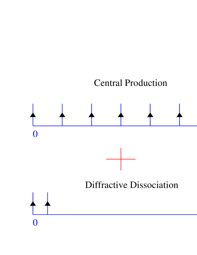
   Figure 25: Structure of the final state in the Eikonal approach.

2. The Eikonal approach gives what we expect from the wave picture of the interaction. Everybody knows that light ( or any other wave process ) interaction with the target gives always a white spot in the middle of the shade. Therefore, we cannot even dream to be consistent with the quantum mechanique without the Eikonal approach. Of course, you can calculate the elastic cross section in the D-L approach considering the elastic cross section as a small perturbation. However, we have to check how small the calculated elastic cross section using the unitarity constraints of Eq. (37) and reconstructing from it the total and inelastic cross sections. Fig. 16 shows that the correction are large and changes the behaviour of $G_{in}(s,b_{t})$.

3. The Eikonal approach is certainly the simplest way of calculating of SC and can be used for the first estimates of how essential they could be. The simplest is not always the best and we will show below that the Eikonal approach has a serious pathology.

4. The Eikonal approach describes well the experimental data on total and elastic cross sections ( see Ref.GLMSOFT and Figs.11 and 17 ).

– ’  s  :

1. In the parton model the Eikonal approach means that only the fastest parton interacts with the target. This is a very unnatural assumption and, in my opinion, it is a great defect of this approach.

2. In the Eikonal approach the errors are of the order of $\frac{\sigma^{SD}}{\sigma_{tot}}\,\,\approx\,\,10-17\%$ and they are not small.

3. The Eikonal approach cannot explain the CDF data on double parton interaction and it give $\sigma_{eff}\,\approx\,30\,mb$ ( see Eq. (88) ) which is in about two times large that experimental value ( see Eq. (85) - Eq. (89) ).

4. The intristic problem of the Eikonal model is the energy behaviour of $\sigma^{SD}$ at large masses $M^{2}\,\,\propto\,\,s$. We will show below that in this region of mass the diffractive cross section $\sigma^{SD}\,\,\propto\,\,s^{\Delta_{P}}$ and it exceeds the value of the total cross section $\sigma_{tot}\,\,\propto\,\,\ln s$. This is our payment for simplicity and unjustified ( $adhoc$ ) assumption that only the fastest parton interacts with the target.

The main assumption of the Eikonal approach is the identification the opacity $\Omega(s,b_{t})$ with the single Pomeron exchange, namely

$$\Omega(s,b_{t})\,=\,POM(s,b_{t})\,\,;$$ (92)

$$POM(s,b_{t})\,\,=\,\,\frac{\sigma_{0}}{\pi R^{2}(s)}\,(\frac{s}{s_{0}})^{\Delta_{P}}\,e^{-\frac{b^{2}_{t}}{R^{2}(s)}}\,\,;$$ (93)

$$R^{2}(s)\,=\,R^{2}_{0}\,\,+\,\,2\alpha^{\prime}_{P}\,\ln(s/s_{0})\,\,;$$ (94)

$$\nu(s)\,\,=\,\,\frac{\sigma_{0}}{\pi R^{2}(s)}\,(\frac{s}{s_{0}})^{\Delta_{P}}\,\,=\,\,\Omega(s,b_{t}=0)\,\,.$$ (95)

Eq. (92) is certainly correct in the kinematic region where $\Omega$ is small or, in other words, at rather small energies or at high energies but al large values of $b_{t}$. Therefore, the Eikonal approach is the natural generalization according to $s$-channel unitarity of the single Pomeron exchange. Using Eq. (37) and Eq. (92) - Eq. (94), one can obtain ( see Ref.GLMSOFT for details ):

$$\sigma_{tot}\,\,=\,\,2\,\pi\,R^{2}(s)\,\{\,\ln(\nu(s)/2)\,\,+\,\,C\,\,-\,Ei(-\nu/2)\,\}\,\,;$$ (96)

$$\sigma_{in}\,\,=\,\,\,\pi\,R^{2}(s)\,\{\,\ln(\nu(s))\,\,+\,\,C\,\,-\,Ei(-\nu)\,\}\,\,;$$ (97)

$$\sigma_{el}(s)\,\,=\,\,\sigma_{tot}(s)\,\,=\,\,\sigma_{in}(s)\,\,;$$ (98)

$$B\,\,=\,\,\frac{d\ln\frac{d\sigma}{dt}}{dt}\,|_{t-0}\,\,=\,\,\frac{R^{2}(s)}{2}\,\frac{hypergeom([1,1,1,],[2,2,2],-\nu/2)}{hypergeom([1,1],[2,2],-\nu/2)}\,\,.$$ (99)

Here, the notations of Maple were used for the generalized hyper geometrical functions. Figs. 11 and 17 show that the Eikonal approach is able to describe the experimental data.

The Eikonal approach gives a very simple procedure how to calculate the survival probability of LRG processes ( see our high energy glossary ). Indeed, in this approach the general formula of Eq. (68) can be simplified and it has a form:

$$<S^{2}>\,\,=\,\,\frac{\int\,d^{2}b_{t}S_{H}(b_{t})\,\,P(s,b_{t})}{\int\,d^{2}b_{t}S_{H}(b_{t})}\,\,=\,\,\frac{\int\,d^{2}b_{t}S_{H}(b_{t})\,\,e^{\Omega(s,b-t)}}{\int\,d^{2}\,b_{t}\,\,S_{H}(b_{t})}\,\,,$$ (100)

where $S_{H}(b_{t})$ is the profile function for the “hard” processes for two jets production. For all numerical estimates we took a Gaussian parameterization for $S_{H}(b_{t})\,=\,\frac{1}{\pi\,R^{2}_{H}}e^{-\frac{b^{2}_{t}}{R^{2}_{H}}}$. In the framework of this simple parameterization all integrals can be taken analytically and we have

$$<S^{2}>\,\,=\,\,\frac{a(s)\,\gamma[a(s),\nu(s)]}{[\,\nu(s)\,]^{a(s)}}\,\,,$$ (101)

with

$$a(s)\,\,=\,\,\frac{R^{2}(s)}{R^{2}_{H}}\,\,=\,\,\frac{interaction\,\,area\,\,for\,\,``soft"\,\,collisions}{interaction\,\,area\,\,for\,\,``hard"\,\,collisions}\,\,>\,\,1\,\,.$$ (102)

$\gamma[a,\nu]$ is incomplete gamma function.

Fig.26 shows the Eikonal model prediction for $<S^{2}>$ which are in a good agreement with the D0 data and reproduce the energy behaviour of the LRG rate( see Fig.9-b ).

Figure 26: $<S^{2}>$ in the Eikonal approach.

The key problem in the Eikonal approach is diffraction production which has not been included in our unitarization procedure. This is a more complicated way to express that DD is equal to zero in the Eikonal approach. However, we can treat the diffraction dissociation as a perturbation considering that its cross section is much smaller than the elastic one. Fig.17 shows that such an approach cannot not be very good since $\frac{\sigma^{DD}}{\sigma_{el}}\,\,\approx\,\,50\%$. The first step is to consider the triple Reggeon diagram of Fig.18-b type $A_{PPP}$. The second one is to take into account the rescatterings of the fast partons which suppress the value of $A_{PPP}$. Actually, the resulting cross section has the same form of the survival probability for LRG processes since the DD is the simplest LRG process:

$$\frac{M^{2}\,d\sigma^{SD}}{dM^{2}}\,|_{t=0}\,\,=\,\,\int\,d^{2}\,b_{t}A_{PPP}(s,M^{2})\,\,P(s,b_{t})\,\,=$$ (103)

$$\frac{\sigma^{2}_{0}}{2\,\pi\,R^{2}_{1}(\frac{s}{M^{2}})}\,G_{PPP}\,\times\,(\,\frac{M^{2}}{s}\,)^{2\,\Delta_{P}}\,(\,\frac{M^{2}}{s_{0}}\,)^{\Delta_{P}}\,\frac{a(s)\,\gamma[a(s),\nu{s}]}{[\nu]^{a(s)}}\,\,,$$

where

$$a(s)\,\,=\,\,\frac{2R^{2}(s)}{R^{2}_{1}(\frac{s}{M^{2}})\,\,+\,\,2\,R^{2}_{1}(\frac{M^{2}}{s_{0}})}$$ (104)

with $R^{2}_{1}(\frac{s}{M^{2}})\,=\,2\,R^{2}_{01}\,+\,r^{2}_{01}\,+\,4\,\alpha^{\prime}_{P}(0)\,\ln(\frac{s}{M^{2}})$. $R^{2}_{01}$ denotes the radius of the proton - Pomeron vertex while $r^{2}_{01}$ is the radius of the triple Pomeron vertex GLMDD . $R^{2}(s)\,=\,4\,R^{2}_{01}\,\,+\,\,4\,\alpha^{\prime}_{P}\ln(s)$.

Eq. (103) describes experimental data much better than the single Pomeron exchange after adding a secondary Reggeon contributions. It shows that we are on the correct way. The most important feature of Eikonal approach description is the flattering of the energy dependence. However, in Fig.17 we plot the integrated cross section over $M^{2}$ defining the region of integration $4\,<\,M^{2}\,0.3\,\sqrt{s\,1\,GeV^{2}}$. the experimental $\sigma^{SD}$ was integrated in the region $4\,<\,M^{2}\,0.05\,s$. We cannot trust our calculations for $M^{2}\,\propto\,s$ since

$$a(s)\,|_{s\,\,\gg\,\,1}\,\longrightarrow\,\,\,2\,\{\,\,1\,\,\,-\,\,\,\frac{\ln M^{2}}{\ln s}\,\,\}\,\,.$$ (105)

Using the asymptotics for the incomplete gamma function we obtain that

$$\frac{M^{2}\,d\sigma^{SD}}{dM^{2}}\,\,\Longrightarrow\,\,(\,M^{2}\,)^{\Delta_{P}}\,\,.$$ (106)

Integrating Eq. (14) over $M^{2}$ up to $M^{2}\,=\,k\,s$ one obtain

$$\sigma^{SD}\,\propto\,\int^{ks}\frac{dM^{2}}{M^{2}}\,(\,M^{2}\,)^{\Delta_{P}}\,\,=\,\,\frac{1}{\Delta_{P}}(\,k\,s\,)^{\Delta_{P}}\,\,\gg\,\,\sigma_{tot}\,\,\propto\,\,\ln s\,\,.$$ (107)

Eq. (16) shows that there is no way to incorporate the diffractive production in the Eikonal model since the “small” parameter of such an approach cannot be small.

This example is the most transparent illustration of the difficult problem in taking into account the SC - the description of high mass diffraction.

V.4 Correct SC ( ? )

Certainly, we do not know an answer to the question what is a correct procedure to take into account SC. Here, I discuss two models for SC which both are better than Eikonal approach.

Quasi-Eikonal Model.

The idea of this model is very simple: to take into account the diffractive dissociation in the same Eikonal way as elastic rescatterings. Doing so, we assume that we have two wave functions which are diagonal with respect to the strong interactions: $\Psi_{1}$ and $\Psi_{2}$. The general Eq. (55) has the form

$$\Psi_{hadron}\,\,\,=\,\,\,\beta_{1}\,\Psi_{1}\,\,\,+\,\,\,\beta_{2}\,\Psi_{2}\,\,\,,$$ (108)

with condition: $\beta_{1}^{2}\,+\,\beta_{2}^{2}\,\,=\,\,1$, which follows from the normalization of the wave function. The wave function of the diffractively produced bunch of hadrons should be orthogonal to $\Psi_{hadron}$ and looks as follows:

$$\Psi_{D}\,\,\,=\,\,\,-\,\beta_{2}\,\Psi_{1}\,\,\,+\,\,\,\beta_{1}\,\Psi_{2}\,\,.$$ (109)

The elastic and single diffraction amplitude in this model can be rewritten, using Eq. (56), Eq. (108) and Eq. (109) in the form:

$$a_{el}(s,b_{t})\,\,=\,\,<\Psi_{final}\ \Psi_{hadron}>\,\,=\,\,\beta^{2}_{1}\,A_{1}\,\,+\,\,\beta^{2}_{2}\,A_{2}\,\,;$$ (110)

$$a_{SD}(s,b_{t})\,\,=\,\,<\Psi_{final}\ \Psi_{D}>\,\,=\,\,\beta_{1}\,\beta_{2}\,\{\,A_{2}\,\,-\,\,A_{1}\,\}\,\,.$$ (111)

For amplitude $A_{n}(s,b_{t})$ we have a unitarity constraint of Eq. (60) and therefore:

$$A_{n}(s,b_{t})\,\,=\,\,i\,\{\,1\,\,-\,\,e^{-\frac{\Omega_{n}(s,b_{t})}{2}}\,\}\,\,;$$ (112)

$$G_{n}(s,b_{t})\,\,=\,\,1\,\,\,-\,\,\,\,e^{-\Omega_{n}(s,b_{t})}\,\,.$$ (113)

Assuming the simplest eikonal form for $\Omega_{n}$ ( see Eq. (92) - Eq. (95) ), namely

$$\Omega_{n}(s,b_{t})\,=\,\frac{\sigma_{0n}}{\pi R^{2}_{n}(s)}\,(\frac{s}{s_{0}})^{\Delta_{P}}\,e^{-\frac{b^{2}_{t}}{R^{2}_{n}(s)}}\,\,,$$ (114)

we have the final answer:

$$\sigma_{tot}\,=\,2\int\,d^{2}b_{t}\{\beta^{2}_{1}\,[\,1\,\,-\,\,e^{-\frac{\Omega_{1}}{2}}\,]\,\,+\,\,(\,1\,-\,\beta^{2}_{1}\,)\,[\,1\,-\,e^{-\frac{\Omega_{2}}{2}}\,]\,\}\,\,;$$ (115)

$$\sigma_{el}\,=\,\int\,d^{2}b_{t}\,[\,\beta^{2}_{1}\,[\,1\,\,-\,\,e^{-\frac{\Omega_{1}}{2}}\,]\,\,+\,\,(\,1\,-\,\beta^{2}_{1}\,)\,[\,1\,-\,e^{-\frac{\Omega_{2}}{2}}\,]\,]^{2}\,\,;$$ (116)

$$\sigma^{SD}\,\,=\,\,\int\,d^{2}b_{t}\,\beta^{2}_{1}\,(\,1\,-\,\beta^{2}_{1})\,[\,e^{-\frac{\Omega_{2}}{2}}\,\,-\,\,e^{-\frac{\Omega_{1}}{2}}\,]^{2}\,\,.$$ (117)

It is obvious from Eq. (115) - Eq. (117) that we introduce three new parameters to describe SC including the processes of diffractive dissociation: $R^{2}_{2}$ $\sigma_{20}$ and $\beta_{1}$. They are correlated with the total cross section of the diffractive dissociation and its $t$- dependence. At first sight it is strange that we have to introduce three parameters not two. The third parameter $\sigma_{02}$ is closely related to the cross section of “elastic” rescattering of the hadrons produced in the diffractive dissociation. The meaning of all parameters is clear from Fig. 27.

Figure 27: The Pomeron exchanges in the Quasi-Eikonal model.

We can rewrite Eq. (115) - Eq. (117) in more convenient form, using the experimental fact that the exponential parameterization works quite well for differential cross section of DD. Indeed, we can assume that

$$\Omega_{2}\,\,-\,\,\Omega_{1}\,\,=\,\,\Omega_{D}(s,b_{t})\,=\,\frac{\sigma_{D0}}{\pi R^{2}_{D}(s)}\,(\frac{s}{s_{0}})^{\Delta_{P}}\,e^{-\frac{b^{2}_{t}}{R^{2}_{D}(s)}}\,\,,$$ (118)

while for $\Omega_{1}$ we use the parameterization of Eq. (114). In such a parameterization we have a very simple form for $a_{el}$ ands $a_{D}$, namely

$$a_{el}(s,b_{t})\,\,=\,\,1\,\,-\,\,e^{-\frac{\Omega_{1}}{2}}\,\,+\,\,(1-\beta^{2}_{1})\,e^{-\frac{\Omega_{1}}{2}}\,\{\,1\,-\,e^{-\frac{\Omega_{D}}{2}}\,\}\,\,;$$ (119)

$$a_{D}(s,b_{t})\,\,=\,\,\beta^{2}_{1}\,(1-\beta^{2}_{1})\,\{\,1\,-\,e^{-\frac{\Omega_{D}}{2}}\,\}\,\,e^{-\frac{\Omega_{1}}{2}}\,\,.$$ (120)

Fig. 28 shows the result of fitting of energy behaviour of different “soft” observables. The parameters, that were used, are

1. $\Delta_{P}$  =  0.1  ;

2. $\frac{\sigma_{10}}{R^{2}_{1}}\,\,=\,\,0.06\,\,\frac{\sigma_{D}}{R^{2}_{D}}\,\,=\,\,\frac{50}{\pi R^{2}_{1}}$  ;

3.$\beta_{2}$= 0.5

4. $R^{2}_{1}\,\,=\,\,26\,\,+\,\,4\,\alpha^{\prime}_{P}(0)\,\ln(s/s_{0})$ with $\alpha^{\prime}_{P}(0)=0.25\,\,GeV^{-2}$.

5. $R^{2}_{D}\,\,=\,\,13\,\,+\,\,4\,\alpha^{\prime}_{P}(0)\,\ln(s/s_{0})$ with $\alpha^{\prime}_{P}(0)=0.25\,\,GeV^{-2}$.

The only parameter which we have to comment is a sufficiently big difference in $\frac{\sigma{0i}}{R^{2}_{i}}$ for elastic and diffractive scattering. We think, that it happened because of the fact that we took effectively into account the integration over produced mass in our parameterization.

Fig. 28-a	Fig. 28-b
Fig. 28-c	Fig. 28-d

Figure 28: The “soft” observables in the Quasi - Eikonal model.

“Fan” diagrams (Schwimmer resummation ).

The technical problem that we are going to solve here is the resummation of all “fan” diagrams (see for example Fig. 18-b and Fig. 29-a). it is interesting to mention that there is a problem which can be solved by such a resummation, namely, the interaction of a fast hadron with heavy nuclei ( see Refs. SCHWIM LR81 ). Indeed, the vertex for Pomeron - nucleus interaction is proportional to $g_{N}\,A$, where $g_{N}$ is the Pomeron-nucleon vertex and $A$ is the atomic number. Therefore, the “fan” diagrams give you the maximal contribution ( $\propto\,(g_{N}G_{3P}A)^{n}$ where $G_{3P}$ is the vertex for triple Pomeron interaction ). Neglecting all momentum transferred dependence in nucleon - nucleon scattering since $R^{2}_{N}\,=\,R^{2}_{0}\,+\,\alpha_{P}(0)\ln(s/s_{0})\,\,\ll\,\,R^{2}_{A}$ we can write a simple equation which sums all “fan” diagrams. The graphic form of this equation is presented in Fig.29-b and it has the following analytical form for p + A interaction at $Y\,=\,\ln(s/s_{0})$:

$$G_{P}(Y,b_{t})\,\,=\,\,g^{2}_{N}AF_{A}(b_{t})\,e^{\Delta_{P}\,\,Y}\,\,-\,\,g_{N}\,G_{3P}\,\,\int^{Y}_{0}\,dy\,\,e^{Y\,-\,y}\,\,G^{2}_{P}(y,b_{t})\,\,.$$ (121)

Fig. 29-a

Fig. 29-b

Figure 29: “Fan” diagrams for nucleon - nucleusa interaction: (a) an example and (b) the graphic form of equation for summation of all “fan” diagrams.

Taking derivative with respect to $Y$ and using Eq. (121) we can reduce this equation to simple differential equation:

$$\frac{d\,G_{P}(Y.b_{t})}{dY}\,\,=\,\,\Delta_{P}G_{P}(y.b_{t})\,\,-\,\gamma\,G^{2}_{P}(Y,b_{t})\,\,,$$ (122)

where $gamma=g_{N}\,G_{3P}\,$. The solution should satisfy the following initial condition which is obvious directly from Eq. (121):

$$G_{P}(Y,b_{t})|_{Y=0}\,\,=\,\,g^{2}_{N}AF_{A}(b_{t})\,\,,$$ (123)

where $F_{A}(b_{t})$ directly related to form factor of a nucleus $F(t)\,\,=\,\,\int\,\,d^{2}b_{t}\,e^{i\,\vec{q}\cdot\vec{b}_{t}}\,\,F_{A}(b_{t})$ with $q^{2}=-t$.

One can obtain the solution:

$$G_{P}(Y,b_{t})\,\,\,=\,\,\frac{g^{2}_{N}\,A\,F_{A}(b_{t})\,\,e^{\Delta_{P}\,Y}}{1\,\,+\,\,g^{2}_{N}\,A\,\,F_{A}(b_{t})\frac{\gamma}{\Delta_{P}}\,\,\{\,e^{\Delta_{P}\,Y}\,\,-\,\,1\,\}}\,\,.$$ (124)

One can see that this solution has a nice properties:

1. If $A\,F_{A}(b_{t})\,e^{\Delta_{P}\,Y}\,\,\gg\,\,1$   $G_{P}\,\,\Longrightarrow\,\,\frac{\Delta_{P}}{\gamma}$  ;

2. If $A\,F_{A}(b_{t})\,e^{\Delta_{P}\,Y}\,\,\ll\,\,1$    $G_{P}\,\,\Longrightarrow\,\,g^{2}_{N}\,A\,F_{A}(b_{t})\,\,e^{\Delta_{P}\,Y}$  ;

3. the equation

   $$g^{2}_{N}\,A\,F_{A}(b_{0})\,\,\frac{\gamma}{\Delta_{P}}\,\,e^{\Delta_{P}\,Y}\,\,=\,\,1$$ (125)

   defines the value of $b_{t}=b_{0}$, which is the border between the above two conditions. Namely, for $b_{t}\,\,<\,\,b_{0}$ the first one holds, while for $b_{t}\,\,>\,\,b_{0}$ the form factor is so small that we are in the region of the second constraint.

4. Talking for simplicity the exponential form for form factor $F_{A}(b_{t})\,\,=\,\,\frac{1}{\pi R^{2}_{A}}\,e^{-\,\frac{b^{2}_{t}}{R^{2}_{A}}}$ we obtain the solution to Eq. (125):

   $$b^{2}_{0}\,\,=\,\,R^{2}_{A}\,\,\Delta_{P}\,Y\,\,\,\ln(g^{2}_{N}\,A\,F_{A}(b_{0})\,\,)\frac{\gamma}{\Delta_{P}})\,\,.$$ (126)

5. From Eq. (126) we can obtain the asymptotic formula for the total cross section:

   $$\sigma_{tot}(nA)\,\,\Longrightarrow\,\,2\pi b^{2}_{0}\,\,\propto\,A^{\frac{2}{3}}\Delta+p\,Y\,\ln(AY)$$ (127)

6. The cross section of the diffractive dissociation turns out to be constant at large $M^{2}\,\sim\,s$. Therefore, this approach has no such difficulties as Eikonal and/or Quasi-Eikonal Model. The reason for this is quite simple: In the Eikonal model we took into account only the rescatterings of the fastest parton (see Fig.18-a ) in the parton cascade. The “fan” diagrams describes the interaction of all partons with the target as it can be seen from Fig.18-b.

7. Eq. (127) gives a nice illustration that we can have an increase in the radius of interaction without assuming any slope for Pomeron trajectory.

The “fan” diagrams gives a rather selfconsistent approach which heal a lot of difficulties but the main problem is to justify this approach. I gave one example - hadron - nucleus collision- for which the problem can be reduced to summation of the “fan” diagrams. You will see more in this lecture.

To finish with hadron - nucleus interaction we have to treat $G_{P}$ as opacity in the eikonal formula $\Omega=G_{P}$ (see Eq. (92) - Eq. (95) ).

II   “H A R D”    P O M E R O N

.

VI EVOLUTION EQUATIONS AT $\mathbf{x}\,\longrightarrow\,\,0$

VI.1 Parton cascade and evolution equations:

As it has been mentioned ( see Eq. (15) - Eq. (14) ) “hard” Pomeron is nothing more than the high energy behaviour of the scattering amplitude at short distances that follow from the pQCD. In spite of the fact that solution of the evolution equations gives nothing like the Regge pole - Pomeron, the parton cascade picture ( see Fig.1 ) is still correct for interpretation. Let me derive for you Eq. (14) and show you that that simple equations (Eq. (1) - Eq. (5) ) work quite well for the “hard” Pomeron too.

The probability to emit one extra gluon in QCD is equal to

$$P_{i}\,\,=\,\,\frac{N_{c}\alpha_{S}(k^{2}_{ti})}{\pi}\,\frac{dx_{i}}{x_{i}}\,\frac{dk^{2}_{ti}}{k^{2}_{ti}}\,\,,$$ (128)

where $x_{i}$ is a fraction of energy carried by gluon $``i"$ and $k_{ti}$ is its transverse momentum. Factor $\frac{dx_{i}}{x_{i}}dk^{2}_{ti}$ is nothing more than the invariant volume for emission ( $d^{3}k_{i}/E_{i}$ ) and the extra $k^{2}_{t}$ comes from the gluon propagator. You can check that Eq. (128) gives the only possible dimensionless combination. Recall, QCD is dimensionless theory.

To calculate the probability to emit $n$ ( $W_{n}$ ) gluons we need to find the product of probabilities, namely

$$W_{n}\,\,=\,\,\prod^{n}_{i=0}\,\,\,P_{i}\,\,,$$ (129)

and to find the probability to emit arbitrary number of gluons we have to sum Eq. (130) over $n$:

$$W\,\,=\,\,\sum^{\infty}_{n=0}\,\,W_{n}\,\,=\,\,\sum^{\infty}_{n=0}\,\,\prod^{n}_{i=0}\,\,\,P_{i}$$ (130)

$$=\,\,\sum^{\infty}_{n=0}\,\,\prod^{n}_{i=0}\,\,\,\frac{N_{c}\alpha_{S}(k^{2}_{ti})}{\pi}\,\frac{dx_{i}}{x_{i}}\,\frac{dk^{2}_{ti}}{k^{2}_{ti}}\,\,.$$

To obtain the deep inelastic structure function we have to integrate over all possible emission with the conditions: $x_{i}\,\,\geq\,\,x_{B}$ and $k^{2}_{i}\,\,\leq\,\,Q^{2}$ where $x_{B}\,\,=\,\,\frac{Q^{2}}{s}$ and $q^{2}$ is the virtuality of the probe. The largest contributions we can obtain from the phase space in which both integrals with respect $xi$ and $k^{3}{ti}$ give logs ( $ln(1/x_{B})$ and $lnQ^{2}$, respectively). This phase space is the following:

$$x_{0}\,\gg\,x_{1}\,\gg\,x_{2}\,\,\gg\,...\,\gg\,x_{i}\,\gg\,x_{i+1}\,\gg\,...\,\gg\,x_{n}\,\gg\,x_{B}\,\,;$$ (131)

$$Q^{2}\,\gg\,k^{2}_{tn}\,\gg\,k^{2}_{t,n-1}\,\gg\,...\,\gg\,k^{2}_{t1}\,\gg\,Q^{2}_{0}\,\,.$$ (132)

Therefore, we have a strong ordering in transverse momenta and fractions of energy. Taking into account Eq. (131) and Eq. (132), we can easily rewrite ( in the simplest case, neglecting $k^{2}$ dependence of QCD coupling constant )

$$\int\prod^{n}_{i=0}\,\frac{N_{c}\alpha_{S}(k^{2}_{ti})}{\pi}\,\frac{dx_{i}}{x_{i}}\,\frac{dk^{2}_{ti}}{k^{2}_{ti}}\,\,=\,\,\frac{1}{n!^{2}}\,\{\,\frac{N_{c}\alpha_{S}(Q^{2}_{0})}{\pi}\,\ln(Q^{2}/Q^{2}_{0})\,\ln(1/x_{B})\,\}^{n}\,\,\,.$$ (133)

Therefore, the structure function can be found just summing all contributions of Eq. (133):

$$xG(x,Q^{2})\,\,=\,\,\sum^{\infty}_{n=0}\,\,\frac{L^{n}}{n!^{2}}\,\,$$ (134)

where scale $L$ is equal to

$$L\,\,\,=\,\,\frac{N_{c}\alpha_{S}(Q^{2}_{0})}{\pi}\,\ln(Q^{2}/Q^{2}_{0})\,\ln(1/x_{B})\,\,=\,\,\xi\,\,y\,\,\,$$ (135)

where $\xi\,\,=\,\,\frac{N_{c}\alpha_{S}(Q^{2}_{0})}{\pi}\,\ln(Q^{2}/Q^{2}_{0})$ and $y=\ln(1/x_{B})$. For large $Q^{2}$ and small $x_{B}$ parameter $L\,\,\gg\,\,1$ and, therefore, only sufficiently large $n$ will be dominant in Eq. (135). Since

$$2n!\,\,=\,\,\Gamma(2n+1)\,\,=\,\,\frac{2^{2n}}{\sqrt{\pi}}\,\Gamma(n+1)\,\,\Gamma(n+\frac{1}{2})\,\,\Longrightarrow\,\,\frac{2^{2n}}{\sqrt{\pi}}(n!)^{2}\,\,$$ (136)

we can rewrite Eq. (134) in the form

$$xG(x,Q^{2})\,\,\Longrightarrow\,\,\sum^{\infty}_{n=0}\,\,\frac{(\,2\,\sqrt{L}\,)^{2n}}{2n!}\,\,=\,\,e^{2\sqrt{L}}$$ (137)

On the other hand, using Stirling formula, we can evaluate

$$2n!\,\,\,\rightarrow\,\,\,(2n)^{2n}\,e^{-2n}\,\,,$$

which, being substituted in Eq. (137) gives the estimate for the average $n$, namely,

$$<n>\,\,=\,\,2\sqrt{L}\,\,.$$ (138)

One can see that Eq. (137) can be written as

$$xG(x,Q^{2})|_{L\,\gg\,\,1}\,\,\Longrightarrow\,\,e^{<n>}\,\,.$$ (139)

For running coupling constant the only difference is the redefinition of the variable $\xi=\ln\frac{\alpha_{S}(Q^{2})}{\alpha_{S}(Q^{2}_{0})}$ in Eq. (135).

VI.2 Why do we use evolution equations?

The first question is what is the meaning of $<n>$. To answer this question we need to look in the picture of our cascade more careful. Let us assume that the number of “wee” partons $N$ is not extremely large or in other words there is only one “wee” parton with definite fraction of energy ($x_{i}$ ) and transverse momentum ($k_{ti}$ ). In this case only one “wee” parton interacts with the target and all others gather together without loosing their coherency. In the Feynman diagrams they contribute to the renormalization of mass and coupling constant in QCD. This is shown in Fig.30.

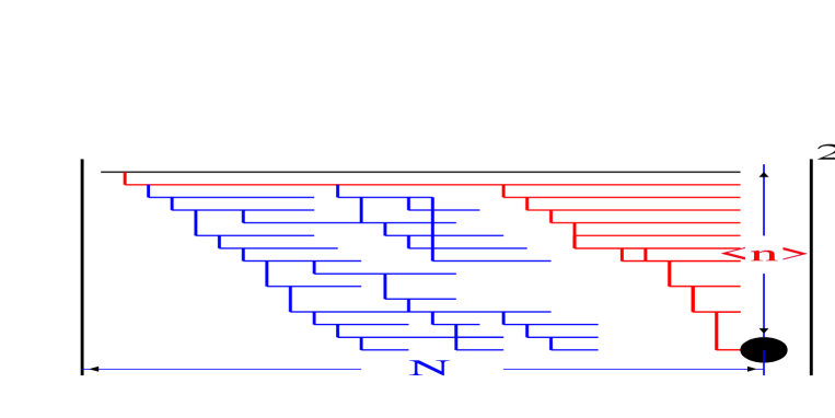
Figure 30: Parton cascade and evolution equation ( Feyman diagrams).

In Fig. 30 one can see that $<n>$ means the average number of cells in our “ladder” diagram or, in other words, in our evolution equations. On the other had, $<n>$ is the average number of produced jets ( mini - jets ) in the whole region of rapidity accessible in the experiment. I found very instructive to plot what we know from HERA experiment about the value of $<n>$ ( see Fig.31 )

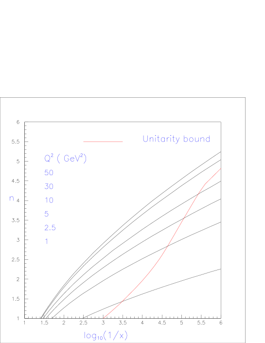
Figure 31: $<n>$ versus $x$ at different values of $Q^{2}$ from HERA experiment.

In Fig. 32 $<n>$ is plotted down to $x\,=\,10^{-6}$ and looking at this plot we can see, that

• $<n>$ increases mostly due to cascading rather in $Q^{2}$ than in $\ln(1/x)$  ;

• The maximum value of $<n>$ is about 5  ;

• $<n>$ is the total multiplicity of produced jets and/or minijets. Therefore, the average density of produced jets ( minijets) is less than $d<n>/dy\,\,\approx\,\,0.5$. This number suggests that we need to calculate only the Feynman diagrams of up to $\alpha^{2}_{S}$ or/and $\alpha^{3}_{S}$ order  ;

• High energy resummation is only a way to get $N$ without calculating $<n>$   .

The main conclusion from this discussion is very simple: we have to use the evolution equations only because it is the only known way how to calculate $N$ without evaluation of $<n>$. However, if we will find a way to calculate $<n>$ we will be able to predict our structure functions with better accuracy restricting yourselves by calculation only limited number of diagrams.

VII SC FOR “HARD” POMERON

The main outcome of our previous discussion is the fact that $N\,\,\gg\,\,1$ at high energies. It happens both for “hard” ( see Eq. (14) and/or Eq. (138)) and “soft” processes. Therefore, in the collisions at high energy the new interesting system of parton has been created with large density of partons. For the “hard” processes all these partons are at the short distances where the coupling QCD constant is small enough to be use as a small parameter. However, we cannot apply for such a system the usual methods of perturbative QCD because the density of partons is large. In essence, the theoretical problems here are non perturbative, but the origin of the non perturbative effects does not lie in long distances and large values of $\alpha_{S}$, which are typical for the confinement region.

VII.1 Which parton density is large?

The quantative estimates of which density is high, we can obtain from the $s$-channel unitarity GLR which we can use in two different form:

• $\sigma_{tot}(\gamma^{*}p)\,\,\leq\,\alpha_{em}\,2\,\pi\,R^{2}$, where $R$ is the size of the target, $\alpha_{em}$ is the fine structure constant ( see Ref. GRIB for explanation why we have $\alpha_{em}$ ). This constraint can be rewritten as GLR MUQI MU90

  $$\kappa\,\,=\,\,\frac{3\,\pi\,\alpha_{S}xG(x,Q^{2})}{Q^{2}\,R^{2}}\,\,\leq\,\,1\,\,.$$ (140)

• $\sigma^{DD}(\gamma^{*}p)\,\,\leq\,\,\sigma_{tot}(\gamma^{*}p)$, where $DD$ stands for diffractive dissociation. This inequality leads also to Eq. (140).

Therefore,

1. If $\kappa$ is very small ($\kappa\ll 1$ ), we have a low density QCD in which the parton cascade can be perfectly described by the DGLAP evolution equations DGLAP ;

2. If $\kappa\,\,\leq\,\,1$, we are in the transition region between low and high density QCD . In this region we can still use pQCD, but have to take into account the interaction between partons inside the partons cascade;

3. If $\kappa\,\,\geq\,\,1$, we reach the region of high parton density QCD, where we need to use quite different methods from pQCD

First, we want to make a remark on parton densities in a nucleus. Taking into account that for nucleus $R_{A}\,\,=\,\,R_{N}\,\times\,A^{\frac{1}{3}}$ and $xG_{A}(x,Q^{2})\,\,=\,\,A\,xG_{N}(x,Q^{2})$, we can rewrite Eq. (140) as

$$\kappa_{A}\,\,=\,\,\frac{3\,\pi\,\alpha_{S}A\,xG_{N}(x,Q^{2})}{Q^{2}\,R^{2}_{N}\,\,A^{\frac{2}{3}}}\,\,=\,\,A^{\frac{1}{3}}\,\kappa_{N}\,\,\leq\,\,1\,\,.$$ (141)

Therefore, for the case of an interaction with nucleii, we can reach a hdQCD region at smaller parton density than in a nucleon .

Fig.32 gives the kinematic plot $(x,Q^{2})$ with the line $\kappa=1$, which shows that the hdQCD effect should be seen at HERA.

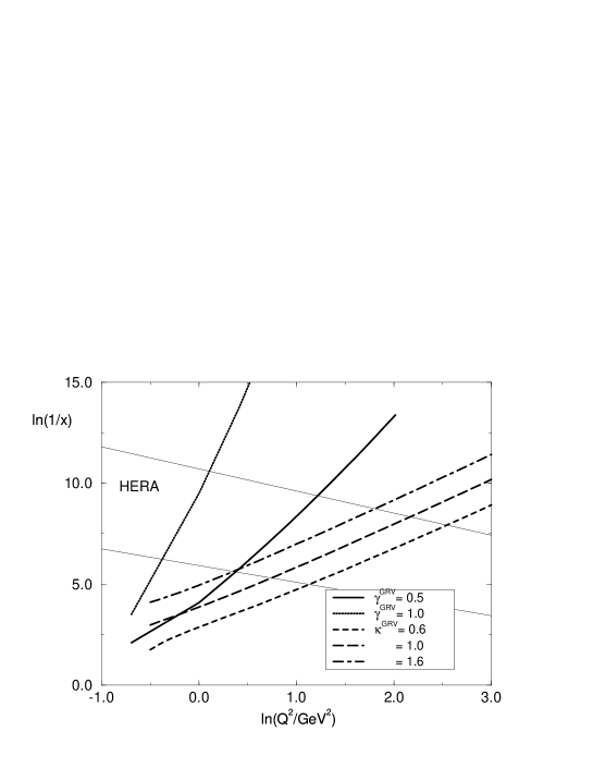
Figure 32: Contours for $<\gamma>$ and $\kappa$ for the GRV’94 gluon density and HERA kinematic region.

VII.2 Two different theoretical approaches

To understand these two approaches we have to look back at Fig.1 which gives you a picture of high energy interaction in the parton approach. In Eq. (1) $N$ is the flux of partons. The main idea of SC is the fact that this flux should be renormalized in the case of high parton density. Indeed, if the number of “wee” partons is so large that, let say, two partons have the same kinematic variables : $x_{i}$ and $\vec{k}_{ti}$, we do not need to take into account the interaction of these two partons two times. Let me recall, that the total cross section is the number of interaction but not the number of partons. It means that if the first of two partons has interacted with the target the total cross section does not depend upon the fact did the second interact or not. It is obvious that the probability to have two partons which could interact with the target semalteneously is equal to

$$P_{2}\,\,=\,\,\frac{\sigma_{0}\,\,N}{\pi R^{2}(x_{i})}\,\,,$$ (142)

where $\pi R^{2}$ is the area which is populated by partons with the fraction of energy $x_{i}$. Therefore, we have to renormalize the flux

$$RENORMALIZED\,\,\,\,FLUX\,\,=\,\,N_{REN}\,\,=\,\,N\,\times\,\{\,1\,\,-\,\,P_{2}\,\}\,\,\,.$$ (143)

One can see that this renormalized flux gives the total cross section in the form:

$$\sigma_{tot}\,\,=\,\,\sigma^{HP}_{tot}\,\,-\,\,\frac{(\,\sigma^{HP}_{tot}\,)^{2}}{\pi\,R^{2}}\,\,,$$ (144)

which is a Glauber formula for SC in the limit of small SC.

If $N\,\,\approx\,\,1$, we expect that the renormalization of the flux will be small, and we use an approach with the following typical ingredients:

$\bullet$ Parton Approach;

$\bullet$ Shadowing Corrections;

$\bullet$ Glauber Approach;

$\bullet$ Reggeon-like Technique;

$\bullet$ AGK cutting rules .

However, when $N\,\,\gg\,\,1$, we have to change our approach completely from the parton cascade to one based on semiclassical field approach, since due to the uncertainty principle $\Delta N\Delta\phi\,\approx\,1$, we can consider the phase as a small parameter. Therefore, in this kinematic region our magic words are:

$\bullet$ Semi-classical gluon fields ;

$\bullet$ Wiezs$\ddot{a}$cker-Williams approximation;

$\bullet$ Effective Lagrangian for hdQCD;

$\bullet$ Renormalization Wilson group Approach.

It is clear, that for $N\,\approx\,\,1$ the most natural way is to approach the hdQCD looking for corrections to the perturbative parton cascade. In this approach the pQCD evolution has been naturally included, and it aims to describe the transition region. The key problem is to penetrate into the hdQCD region where $\kappa$ is large. Let us call this approach “pQCD motivated approach ”.

For $N\,\gg\,\,1$, the most natural way of doing is to use the effective Lagrangian approach, and remarkable progress has been achieved both in writing of the explicit form of this effective Lagrangian, and in understanding physics behind it MCLER . The key problem for this approach was to find a correspondence with pQCD. This problem has been solved KOV .

Fig.33 shows the current situation on the frontier line in the offensive on hdQCD.

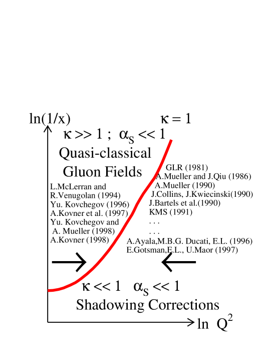
Figure 33: The current situation in the battle for hdQCD.

VII.3 The picture of interaction

To understand the picture of interaction in the region of small $x$ it is better to by examine the parton distribution in the transverse plane (see Fig.those partons with size $r_{p}\,\sim\,\frac{1}{Q}$. At $x\,\ approx\,1$ a few parton are distributed in the hadron disc. If we choose $Q$ such that $r^{2}_{p}\,\ll\,R^{2}_{h}$ then the distance between partons in the transverse plane is much larger than their size, and we can neglect the interaction between partons. The only essential process is the emission of partons,which has been taken into account in QCD evolution. As $x$ decreases for fixed $Q^{2}$ , the number of partons increases. and at value of $x=x_{cr}$, partons start to populate the whole hadron disc densely. For $x\,<\,x_{cr}$ the partons overlap spatially and begin to interact throughout the disc. For such small $x$ values, the processes of recombination and annihilation of partons should be as essential as their emission. However, neither process is incorporated into any evolution equation. What happens in the kinematic region $x\,<\,x_{cr}$ is anybody’s guess. We suggested that parton density saturates, i.e. the parton density is constant in this domain.

VII.4 The GLR equation

The first attempt to take into account the parton - parton interaction in the pQCD motivated approach was done long ago GLR . It was based on the simple idea that there are two processes in a parton cascade (see Fig.1) : (i) the probability of the emission of an extra gluon is proportional to $\alpha_{S}\,\rho$ where $\rho$ is the density of gluon in the transverse plane, namely

$$\rho\,\,=\,\,\frac{xG(x,Q^{2})}{\pi\,R^{2}}\,\,;$$ (145)

and (ii) the annihilation of a gluon, or in other words a process in which the probability is proportional to $\rho^{2}\,\times\,\sigma_{annihilation}$. $\sigma_{annihilation}$ can be estimated as $\sigma_{annihilation}\,\propto\,\alpha_{S}\,r^{2}$, where $r$ is the size of the parton produced in the annihilation process. For deep inelastic scattering, $r^{2}\,\,\propto\,\,\frac{1}{Q^{2}}$. Therefore, in the parton cascade we have

$$Emission\,\,(\,\,1\,\,\rightarrow\,\,2\,\,)\,:\,\,\,probability\,\,=\,\,P^{emission}\,\,\propto\,\,\alpha_{S}\,\,\rho\,\,;$$ (146)

$$Annihilation\,\,(\,\,2\,\,\rightarrow\,\,1\,\,)\,:\,\,\,probability\,\,=\,\,P^{annihilation}\,\,\propto\,\,\alpha^{2}_{S}\,\,\frac{1}{Q^{2}}\,\,\rho^{2}\,\,.$$ (147)

At $x\,\sim\,1$ only emission of new partons is essential, because $\rho\,\ll\,1$ and this emission is described by the DGLAP evolution equations. However, at $x\,\rightarrow\,0$ the value of $\rho$ becomes so large that the annihilation of partons becomes important, and so the value of $\rho$ is diminished. The competition of these two processes we can write as an equation for the number of partons in a phase space cell ( $\Delta y\,=\,\Delta\,\ln(1/x)\,\Delta\,\ln(Q^{2}/Q^{2}_{0})$ ):

$$\frac{\partial^{2}\rho}{\partial\ln(1/x)\partial\ln(Q^{2}/Q^{2}_{0})}\,\,=\,\,\frac{\alpha_{S}\,N_{c}}{\pi}\,\rho\,\,-\,\,\frac{\alpha^{2}_{S}\,\,\tilde{\gamma}}{Q^{2}}\,\,\rho^{2}\,\,,$$ (148)

or in terms of the gluon structure function $xG(x,Q^{2})$

$$\frac{\partial^{2}xG(x,Q^{2})}{\partial\ln(1/x)\partial\ln(Q^{2}/Q^{2}_{0})}\,\,=\,\,\frac{\alpha_{S}\,N_{c}}{\pi}\,xG(x,Q^{2}\,\,-\,\,\frac{\alpha^{2}_{S}\,\,\tilde{\gamma}}{\pi R^{2}\,\,Q^{2}}\,\,(\,xG(x,Q^{2})\,)^{2}\,\,.$$ (149)

This is the GLR equation which gave the first theoretical basis for the consideration of hdQCD. This equation describes the transition region at very large values of $Q^{2}$, but a glance at Fig.32 shows that we need a tool to penetrate the kinematic region of moderate and even small $Q^{2}$.

VII.5 Glauber - Mueller Approach

We found that it is very instructive to start with the Glauber approach to SC. The idea of how to write the Glauber formula in QCD was originally formulated in two papers Ref.LR87 and Ref. MU90 . However, the key paper for our problem is the second paper of A. Mueller, who considered the Glauber approach for the gluon structure function. The key observation is that the fraction of energy, and the transverse coordinates of the fast partons can be considered as frozen, during the high energy interaction with the target LR87 MU90 . Therefore, the cross section of the absorption of gluon($G^{*}$) with virtuality $Q^{2}$ and Bjorken $x$ can be written in the form:

$$\sigma^{N}_{tot}(\,G^{*}\,)\,\,=\,\,$$ (150)

$$\int^{1}_{0}dz\,\,\int\,\frac{d^{2}r_{t}}{2\pi}\,\,\int\frac{d^{2}b_{t}}{2\pi}\Psi^{G^{*}}_{\perp}(Q^{2},r_{t},x,z)\,\,\sigma_{N}(x,r^{2}_{t})\,\,\,\,[{\Psi^{G^{*}}_{\perp}}(Q^{2},r_{t},x,z)]^{*}\,,$$

where $z$ is the fraction of energy which is carried by the gluon, $\Psi^{G^{*}}_{\perp}$ is the wave function of the transverse polarized gluon, and $\sigma_{N}(x,r^{2}_{t})$ is the cross section of the interaction of the $GG$- pair with transverse separation $r_{t}$ with the nucleus. Mueller showed that Eq. (10) can be reduced to

$$xG^{MF}(x,Q^{2})=\frac{4}{\pi^{2}}\int^{1}_{x}\frac{dx^{\prime}}{x^{\prime}}\int_{\frac{1}{Q^{2}}}^{\infty}\frac{d^{2}r_{t}}{\pi r_{t}^{4}}\int_{0}^{\infty}\frac{d^{2}b_{t}}{\pi}2\left\{1-e^{-\frac{1}{2}\,\sigma_{N}^{GG}(x^{\prime},r^{2}_{t})S(b^{2}_{t})}\right\}$$ (151)

with

$$\sigma_{N}^{GG}\,\,=\,\,\frac{4\,\pi^{2}\,\alpha_{S}}{3}\,\,r^{2}_{t}\,xG^{DGLAP}(x,\frac{1}{r^{2}_{t}})\,\,$$

and profile function $S(b_{t})$ chosen in the Gaussian form: $S(b^{2}_{t})\,\,=\,\,\frac{1}{\pi R^{2}}\,\,e^{-\,\frac{b^{2}_{t}}{R^{2}}}\,\,.$

Obviously, the Mueller formula has a defect, namely, only the fastest partons ($GG$ pairs) interact with the target. This assumption is an artifact of the Glauber approach, which looks strange in the parton picture of the interaction. Indeed, in the parton model we expect that all partons not only the fastest ones should interact with the target. At first sight we can solve this problem by iteration Eq. (151)( see Ref. AGL ). It means that the first iteration will take into account that not only the fastest parton, but the next one will interact with the target, and so on.

VII.6 Why equation?

We would like to suggest a new approach based on the evolution equation to sum all SC. However, we want to argue first, why an equation is better than any iteration procedure. To illustrate this point of view, let us differentiate the Mueller formula with respect to $y\,=\,\ln(1/x)$ and $\xi\,=\,\ln Q^{2}$. It is easy to see that this derivative is equal to

$$\frac{\partial^{2}xG(x,Q^{2})}{\partial y\,\partial\xi}\,\,=\,\,\frac{4}{\pi^{2}}\,\int db^{2}_{t}\,\,\{\,\,1\,\,-\,\,e^{-\,\frac{1}{2}\,\sigma(x,r^{2}_{\perp}\,=\,\frac{1}{Q^{2}})\,S(b^{2}_{t})}\,\,\}\,\,.$$ (152)

The advantages of Eq. (152) are

• Everything enters at small distances  ;

• Everything is under theoretical control  ;

• Everything that is not known ( mostly non perturbative ) is hidden in the initial and boundary condition.

Of course, we cannot get rid of our problems changing the procedure of solution. Indeed, the non-perturbative effects coming from the large distances are still important, but they are absorbed in the boundary and initial conditions of the equation. Therefore, an equation is a good ( correct ) way to separate what we know ( short distance contribution) from what we don’t ( large distance contribution).

VII.7 Equation

We suggest the following way to take into account the interaction of all partons in a parton cascade with the target. Let us differentiate the $b_{t}$-integrated Mueller formula of Eq. (151) in $y\,=\,\ln(1/x)$ and $\xi=\ln(Q^{2}/Q^{2}_{0})$. It gives

$$\frac{\partial^{2}xG(y,\xi)}{\partial y\partial\xi}\,\,=\,\,\frac{2\,Q^{2}R^{2}}{\pi^{2}}\,\,\,\left\{\,\,C\,\,+\,\,\ln(\kappa_{G}(x^{\prime},Q^{2}))\,\,+\,\,E_{1}(\kappa_{G}(x^{\prime},Q^{2}))\right\}\,\,\,,$$ (153)

where $\kappa_{G}(x,Q^{2})$ is given by

$$\kappa(x,Q^{2})\,\,=\,\,\frac{N_{c}\alpha_{S}\pi}{2Q^{2}R^{2}}\,xG(x,Q^{2})\,\,.$$ (154)

Therefore, we consider $\kappa_{G}$ on the l.h.s. of Eq. (153) as the observable which is written through the solution of Eq. (153).

Eq. (153) can be rewritten in the form ( for fixed $\alpha_{S}$ )

$$\frac{\partial^{2}\kappa_{G}(y,\xi)}{\partial y\partial\xi}\,\,+\,\,\frac{\partial\kappa_{G}(y,\xi)}{\partial y}\,\,=$$ (155)

$$\,\,\frac{N_{c}\,\alpha_{S}}{\pi}\,\,\left\{\,\,C\,\,+\,\,\ln(\kappa_{G})\,\,+\,\,E_{1}(\kappa_{G})\right\}\,\,\equiv\,\,F(\kappa_{G})\,\,.$$

This is the equation which we propose.

This equation has the following desirable properties:

1. It sums all contributions of the order $(\,\alpha_{S}\,y\,\xi\,)^{n}$, absorbing them in $xG(y,\xi)$, as well as all contributions of the order of $\kappa^{n}$. Therefore, this equation solves the old problem, formulated in Ref.GLR , and for $N_{c}\,\rightarrow\,\infty$ Eq. (155) gives the complete solution to our problem, summing all SC  ;

2. The solution of this equation matches with the solution of the DGLAP evolution equation in the DLA of perturbative QCD at $\kappa\,\rightarrow\,0$  ;

3. At small values of $\kappa$ ( $\kappa\,<\,1$ ) Eq. (155) gives the GLR equation. Indeed, for small $\kappa$ we can expand the r.h.s of Eq. (155) keeping only the second term. Rewriting the equation through the gluon structure function we obtain the GLR equation GLR with the coefficient in front of the second term as calculated by Mueller and Qiu MUQI   ;

4. The first iteration of this equation gives the Mueller formula ( see Ref. MU90 )  ;

5. In general, everything that we know about SC is included in Eq. (155)  ;

VII.8 The size of SC

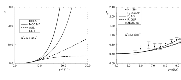
Figure 34: The estimates of SC based on Eq. (155).

In Fig.34 we plot our calculation for the DGLAP evolution equation, for the Glauber - Mueller approach, for the GLR equation and for the new evolution equation. We can conclude, that:

1. SC even in the Glauber - Mueller approach are essential for the gluon structure function  ;

2. The Glauber - Mueller approach considerably underestimates the value of SC  ;

3. The GLR equation leads to stronger SC than the solution to Eq. (155)  ;

4. The new evolution equation does not reproduce the saturation of the gluon density in the region of small $x$ which the GLR equation leads to  .

We firmly believe that the new evolution equation gives the correct way of evaluation of the value of SC. However, the difficult question arises: why the SC have not been seen at HERA? Our answer is:

1. The value of SC is rather large but only in the gluon structure function while their contribution to $F_{2}$ is rather small AGL (see Fig.34 ), and cannot be seen on the background of the experimental errors  ;

2. The theoretical determination of the gluon structure function is not very precise and we evaluate the errors as 50% LERIHC and the SC in $xG$ is hidden in such large errors  ;

3. The statement that SC have not been seen is also not quite correct. Our estimates GLMSLOPEF2 show that the contribution of SC is rather large in the $F_{2}$ slope and incorporating the SC one can describe the recent experimental data DATACOLD on $\frac{\partial F_{2}(x,Q^{2})}{\partial\ln(Q^{2}/Q^{2}_{0})}$ (see Ref.GLMSLOPEF2 for detail ).

VII.9 Effective Lagrangian Approach.

Deeply in my heart, I firmly believe that there will be a bright future for the effective Lagrangian approach in which one combines the physics of hdQCD, with the formal methods of the quantum field theory, and gives a way to incorporate the lattice calculation for the non-perturbative observables. However, the parameter or better to say a new scale $Q^{2}_{0}(x)$ which is the solution of the equation $\kappa(x,Q^{2}_{0}(x))\,\,=\,\,1$ only can be found in the pQCD motivated approach, since the effective Lagrangian was only derived and justified assuming this new scale.

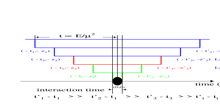
Figure 35: The space - time structure of the parton cascade.

Here, I would like to show what kind of physics have been used to obtain the effective Lagrangian. The space - time picture of the parton cascade is given in Fig.35. The main and very important feature of this cascade is that in the region of low $x$ ( in so called leading log (1/x) approximation of pQCD ) is the fact that a parton with higher energy in the cascade lives much longer than a parton with smaller energy. Let us look for the interaction of the parton emitted at time $t^{\prime}_{2}$. This parton lives much shorter time than all partons emitted before. Therefore, all these emitted before partons will have enough time form a current which depends on their density. We assume that this density is large and because of this fact our current actually is a normal classical current. Finally, the Lagrangian of the interaction of the parton emitted at time $t^{\prime}_{2}$ can be written as

$$L(\rho)\,\,+\,\,j_{\mu}(\rho)\cdot A_{\mu}\,\,+\,\,L(A)\,\,,$$

where $A$ is the field of a parton emitted at $t^{\prime}_{2}$. However, we can consider a parton emitted at $t=t^{\prime}_{3}$ and include the previous one in the system with density $\rho$. The form of Lagrangian should be the same. This is a very strong condition on the form of Lagrangian, so called Wilson renormalization group approach. In Ref.MCLER , this approach has been used to obtain the effective Lagrangian.

III T H E    B F K L    P O M E R O N

VIII The BFKL parton cascade and its evolution.

The BFKL Pomeron BFKL is an asymptotic of the scattering amplitude in perturbative QCD in the kinematic region where the log scale $L\,\,=\,\,\alpha_{S}\,\ln(1/x)\,\,\gg\,\,1$ but the values of virtualities of incoming particles are moreless the same $Q^{2}_{0}\,\,\sim\,\,Q^{2}$. Practically, this means that we calculate the same diagrams as before but in the kinematic region where Eq. (138) holds while there is no special requirements for transverse momentum integration ( there is no Eq. (139) ). Of course, the BFKL Pomeron should match the “hard” Pomeron in the situation when $Q^{2}\,\,gg\,\,Q^{2}_{0}$.

First thing, that I would like to stress is the fact that the origin of the $ln(1/x)$ contributions is very simple. As it has been mentioned the factor $dx_{i}/x_{i}$ in Eq. (128) comes from the phase space. Therefore, if we write the optical theorem for total cross section of two particles with virtualities $Q^{2}$ and $Q^{2}_{0}$ in the form

$$\sigma_{tot}(x,Q^{2},Q^{2}_{0})\,\,=\,\,\sum^{\infty}_{n=2}\,\int\prod_{i}\frac{dx_{i}}{x_{i}}d^{2}k_{ti}|M_{2\,\rightarrow n}(x_{i},k_{i})|^{2}$$ (156)

on can see that to obtain $log(1/x)$ contribution we can safely put all $x_{i}=0$ in amplitudes $M_{n}$. It gives

$$\sigma_{tot}(x,Q^{2},Q^{2}_{0})\,\,=\,\,\sum^{\infty}_{n=0}\,\int\prod_{i}\frac{dx_{i}}{x_{i}}\,\times\,\int d^{2}k_{ti}|M_{2\,\rightarrow\,2+n}(0,k_{i})|^{2}\,\,=$$ (157)

$$\,\,\sum^{\infty}_{n=2}\,\frac{\ln^{n}(1/x)}{n!}\int\,\prod^{n}_{i}d^{2}k_{ti}\,|M_{2\,\rightarrow\,2+n}(0,k_{i})|^{2}\,\,.$$

Deriving Eq. (157) we used the ordering in $x_{i}$ of Eq. (138).

Assuming that the integral over $k_{ti}$ in Eq. (157) gives $\int\prod^{n}_{i}d^{2}k_{ti}\,|M_{2\,\rightarrow\,2+n}(0,k_{i})|^{2}\,\,=\,\,\omega^{n}_{L}$ we can easily obtain that

$$\sigma_{tot}(x,Q^{2},Q^{2}_{0})\,\,=\,\,\frac{\sigma_{0}}{\sqrt{Q^{2}\,Q^{2}_{0}}}\,\,\,\,\,\,(\frac{1}{x}\,)^{\omega_{L}}\,\,,$$ (158)

where $\omega_{L}\,\,\propto\,\alpha_{S}$. The result of Eq. (158) can be rewritten in the form $\sigma_{tot}\,\,\propto\,\,e^{<n>}$ with $<n>=\omega_{L}\,\ln(1/x)$. Note, that factor in front can be obtained just from dimension of the total cross section and the fact that the scattering amplitude in the region of $Q^{2}\,\,\approx\,\,Q^{2}_{0}$ should be symmetric with respect to $Q^{2}\,\rightarrow\,\,Q^{2}_{0}$ and $Q^{2}_{0}\,\rightarrow\,Q^{2}$.

It is interesting to point out that the simple feature of QCD,namely, the fact that we have a dimensionless coupling constant in QCD. In such theory each emission leads to the change of the $\ln k_{t}$ of a parton by some value ( $d$ ) :

$$\Delta\ln(k^{2}_{ti}/Q^{2}_{0})\,\,=\,\,d\,\,.$$ (159)

After $n$- emissions the total change of the transverse momentum will be equal to;

$$<\ln^{2}\,\,(k^{2}_{ti}/Q^{2}_{0})>|_{after\,\,\,n\,\,\,\,emissions}\,\,=\,\,d\,n\,\,.$$ (160)

It means that in average for the scattering amplitude we have

$$<\ln^{2}\,\,(Q^{2}/Q^{2}_{0})>\,\,=\,\,d\,<n>\,\,=\,\,d\,\omega_{L}\ln(1/x)\,\,=\,\,4\,D\,\ln(1/x)\,\,.$$ (161)

Therefore, the transverse momentum dep[endence of the scattering amplitude is a distribution with $<ln(Q^{2}/Q^{2}_{0})>$ given by Eq. (160).

Collecting everything that has been discussed we have

$$\sigma_{tot}(x,Q^{2},Q^{2}_{0})\,\,=\,\,\frac{\sigma_{0}}{\sqrt{Q^{2}\,Q^{2}_{0}}}\,\,\,\,e^{\omega_{L}\,Y}\,\,\frac{1}{\sqrt{4\,D\,\pi\,Y}}\,\,\,\,e^{-\frac{\ln^{2}(Q^{2}/Q^{2}_{0})}{4\,D\,Y}}\,\,.$$ (162)

Eq. (162) gives the answer. The values of three constants: $\sigma_{0}\,\,=\,\,\alpha^{4}_{S}$  ,    $\omega_{L}\,\,\propto\,\,\alpha_{S}$   and  $D\,\,\propto\,\,\alpha_{S}$ have been found in the BFKL approach to perturbative QCDBFKL . It should be stressed that we have used heavily a fact that out theory has no dimension scale. Actually, it has because the QCD coupling depends on the transverse momentum. Therefore, strictly speaking, Eq. (162) is valid only for fixed QCD coupling.

IX The BFKL equation.

IX.1 $\mathbf{\alpha}_{S}(Q^{2}_{0})$ fixed.

This section will be a bit more formal than everything that was before. Nevertheless, I would like to share with you a beautiful result, that the “soft” Pomeron might be the BFKL Pomeron with running QCD coupling + confinement.

The natural function for which the BFKL equation can be written is the gluon density $\phi(y,q^{2})$ which is closely related to the gluon structure function.

$$xG(x,Q^{2})\,\,=\,\,\int^{Q^{2}}\,\,\alpha_{S}(q^{2})\,\phi(y,q^{2})\,\,,$$ (163)

where we introduce from the beginning a new symmetric variable $y=\ln\frac{s}{QQ_{0}}$. In the leading order $y$ is equal to $y=\ln(1/x)$ but in the next to leading order this variable turns out yo be much more convenient.

The BFKL equation BFKL has a form:

$$\frac{d\phi(y,q^{2})}{dy}\,\,=$$ (164)

$$\,\,\delta^{(2)}((\,\vec{q}\,\,-\,\,\vec{q}_{0}\,)\,\,\,+\,\,\int\,\,d^{2}\,q^{\prime}\,K(\,\vec{q},\vec{q}^{\prime}\,)\,\phi(\,y,\,\vec{q}^{\prime},\vec{q}_{0})\,)\,\,-\,\,2\,\alpha_{G}(q^{2})\,\phi(\,y,\,\vec{q},\vec{q}_{0})\,)\,\,,$$

where all notations are clear from Fig.36.

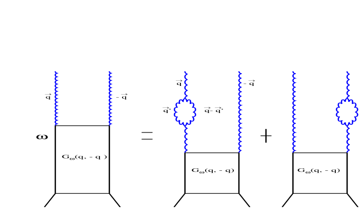
Figure 36: The BFKL equation.

The BFKL kernel has a remarkable property that function

$$\phi_{f}(q^{2})\,\,=\,\,\frac{1}{\sqrt{q^{2}}}\,(\,q^{2}\,)^{f}\,\,$$ (165)

is an eigenfunction, namely

$$\int\,\,d^{2}\,q^{\prime}\,K(q,q^{\prime})\,\phi_{\omega}(q^{\prime})\,\,=\,\,\omega(f)\,\phi_{f}(q^{2})\,\,,$$ (166)

with

$$\omega(f)\,\,=\,\,\frac{N_{c}\alpha_{S}(Q^{2}_{0})}{\pi}\,\{\,\Psi(f)+\Psi(1-f)-2\Psi(1)\,\}\,\,=$$ (167)

$$\,\,\omega_{L}\,\,+\,\,D(f-\frac{1}{2})^{2}\,\,+\,\,O((f-\frac{1}{2})^{3})\,\,,$$ (168)

where $\Psi(z)\,\,=\,\,\frac{d\ln\Gamma(z)}{dz}$ ($\Gamma(z)$ is the Euler gamma-function. For the Mellin transform of $\pi$

$$\phi(y,q^{2})\,\,=\,\,\int^{a+i\infty}_{a-i\infty}\,\,\frac{d\,\omega}{2\,\pi\,i}\,\,e^{\omega\,y}\,G_{\omega}(q^{2})$$ (169)

the BFKL equation reduces to the simple form:

$$\omega\,G_{\omega}(f)\,\,=\,\,1\,\,+\,\,\,\omega(f)\,G_{\omega}(f)\,\,,$$ (170)

where

$$G_{\omega}(q^{2})\,\,=\,\,\int^{a+i\infty}_{a-i\infty}\,\,\frac{d\,f}{2\,\pi\,i}\,\,e^{-f\,(r-r_{0})}\,\,G_{\omega}(f)\,\,,$$ (171)

with $r-r_{0}=ln(Q^{2}/Q^{2}_{0})$.

Substituting solution to Eq. (170) $G_{\omega}(f)\,\,=\,\,\frac{1}{\omega-\omega(f)}$ into Eq. (169) and Eq. (171), we obtain after integration over $\omega$ since we can close contour on the pole in $\omega$

$$\phi(y,q^{2})\,\,=\,\,\int^{a+i\infty}_{a-i\infty}\,\,\frac{d\,f}{2\,\pi\,i}\,\,e^{\omega(f)\,y\,\,-\,\,f\,(r-r_{0})}\,\,G_{\omega}(f)\,\,,$$ (172)

where $G_{\omega}(f)$ should be found from initial nonperturbative parton distributions. Using the expansion of $\omega(f)$ at $f\,\rightarrow\,\frac{1}{2}$, one can see that we are able to take the integral by saddle point method and obtain the answer of Eq. (162) with

$$\omega_{L}\,\,=\,\,\frac{N_{c}\alpha_{S}(Q^{2}_{0})}{\pi}\,4\,\ln 2\,\,;$$ (173)

$$D\,\,=\,\,\frac{N_{c}\alpha_{S}(Q^{2}_{0})}{\pi}\,14\,\zeta(3)\,\,.$$ (174)

IX.2 Running QCD coupling.

The previous subsection was written mostly because I would like to point out that the running QCD coupling leads to a result which is very important since it gives the only theoretical way that I know to obtain the Pomeron - a Reggeon with intercept bigger than 1. Indeed, let us consider the BFKL kernel to be proportional to the running $\alpha_{S}(q^{2})\,\,=\,\,\frac{\alpha_{s}(Q^{2}_{0}))r_{0}}{r}$ where $r_{0}\,=\,lnQ^{2}_{0}/\Lambda^{2})$ and $r\,=\,lnQ^{2}/\Lambda^{2})$ . $\Lambda^{2}$ is the position of Landau pole in $\alpha_{S}$ where QCD coupling constant becomes very large. The generalized BFKL equationRUNBFKL looks as follows:

$$\frac{d\phi(y,q^{2})}{dy}\,\,=$$ (175)

$$\delta^{(2)}((\,\vec{q}\,\,-\,\,\vec{q}_{0}\,)\,\,\,+\,\,\frac{r_{0}}{r}\,\,\int\,\,d^{2}\,q^{\prime}\,K(\,\vec{q},\vec{q}^{\prime}\,)\,\phi(\,y,\,\vec{q}^{\prime},\vec{q}_{0})\,)\,\,.$$

This equation can be easily rewritten as the differential equation in double Mellin transform with respect to $y$ and $r$ ( see Eq. (165) ).

$$-\,\omega\frac{dg(\omega,f)}{df}\,\,=\,\,r_{0}\,\omega_{conf}(f)\,g(\omega,f)\,\,+\,\,r_{0}\,e^{-fr_{0}}\,\,.$$ (176)

The solution of homogeneous equation ( Eq. (176) without the last term ) can be easily found and it has the form ( see Refs. RUNBFKL for details ):

$$g(\omega,f)\,\,=\,\,\tilde{g}(\omega)\,e^{-\,\frac{r_{0}}{\omega}\,\int^{f}_{f_{0}}\,\omega_{conf}(f^{\prime})df^{\prime}}\,\,.$$ (177)

Function $\tilde{g}(\omega)$ should be specified from initial or boundary conditions. The value of $f_{0}$ can be arbitrary since its redefinition is included in function $\tilde{g}(\omega)$. Unless it is specially stipulated $f_{0}$ = 0.

Let us find a Green function of the BFKL equation with running QCD coupling ( $G_{r}(y,r)$ ) which satisfies the following boundary condition:

$$G_{r}(y,r):$$ (178)

$$G_{r}(y,r=r_{0})\,\,=\,\,\delta(y\,-\,y_{0})$$

This Green function allows us to find us the solution of the BFKL equation for any boundary input distribution $G_{in}(y,q^{2}=q^{2}_{0})$ at $q^{2}=q^{2}_{0}$ ( $r=r_{0}$ ). Indeed, such a solution is equal to

$$G(y,r)\,\,=\,\,\int\,dy_{0}\,G_{r}(y,r)\,G_{in}(y_{0},q^{2}=q^{2}_{0})\,\,.$$ (179)

Such a Green function is very useful for study of the boundary condition for the DGLAP evolution. Using $G_{r}(y,r)$ and Eq. (179), we can investigate the $y$-dependence at $q^{2}\,\cong\,q^{2}_{0}$. We can distinguish two cases with different solutions:

1. The integral over $y_{0}$ depends mostly on properties of input function $G_{in}$;

2. The integral over $y_{0}$ is sensitive to the Green function. In this case we can claim that the energy behaviour of our boundary condition is defined by the BFKL dynamics.

Therefore, this Green function ( $G_{r}(y,r)$ ) can provide us with an educated guess for the energy dependence of the boundary condition in the DGLAP evolution equations DGLAP .

Substituting in Eq. (177) the expansion of $\omega_{conf}$ at $f\,\rightarrow\,\frac{1}{2}$ ( see Eq. (168) ) we obtain that integral over $f$ in Eq. (177) gives the Airy function $Ai\left((\frac{\omega}{r_{0}D})^{\frac{1}{3}}\,[\,r\,-\,\frac{\omega_{L}}{\omega}r_{0}\,]\,\right)$. Therefore to satisfy the boundary condition of Eq. (178) we have to choose a function $\tilde{g}(\omega)\,=\,Ai^{-1}\left((\frac{\omega}{r_{0}D})^{\frac{1}{3}}\,[\,r_{0}\,-\,\frac{\omega_{L}}{\omega}r_{0}\,]\,\right)$.

Finally RUNBFKL , $G_{r}(y-y_{0},r,r_{0})$ is equal to

$$G_{r}(y-y_{0},r,r_{0})\,\,=$$ (180)

$$\,\,\sqrt{\frac{r}{r_{0}}}\,\int^{a+i\infty}_{a-i\infty}\,\frac{d\omega}{2\pi i}\,e^{\omega\,(y-y_{0})}\,\,\frac{Ai\left((\frac{\omega}{r_{0}D})^{\frac{1}{3}}\,[\,r\,-\,\frac{\omega_{L}}{\omega}r_{0}\,]\,\right)}{Ai\left((\frac{\omega}{r_{0}D})^{\frac{1}{3}}\,[\,r_{0}\,-\,\frac{\omega_{L}}{\omega}r_{0}\,]\,\right)}\,\,.$$

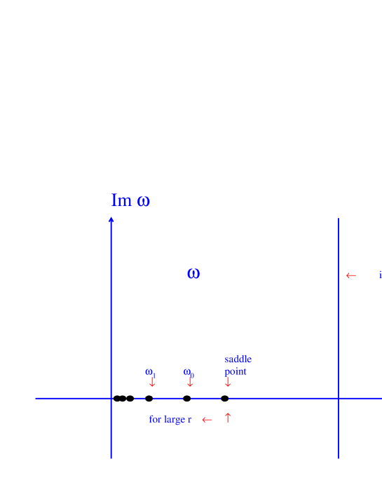
Figure 37: Singularities in $\omega$-plane for the BFKL equation with running QCD coupling.

Airy function is an analytical function which has zeros and a singular behaviour at large values of the argument $Ai(z)|_{z\,>\,0;|z|\,\gg\,1}\,\,\rightarrow\,\,\frac{1}{2z^{\frac{1}{4}}}e^{-\frac{2}{3}\,z^{\frac{3}{2}}}$. Therefore, we have two possibility to take the integral over $\omega$ (see Fig.37, which shows the structure of singularities in $\omega$ - plane ):

1. To draw contour through the saddle point  ;

2. To close contour on the zeros of the denominator  .

It turns out that the position of the saddle point $\omega_{SP}\,=\,\omega_{L}(r_{0})\,\frac{r_{0}}{r_{0}+r}$ and at large values of $q^{2}$ ( $r$ ) it moves to the left. Therefore, for large $r$ the rightmost singularity is the $\omega_{0}(r_{0})$ - the zero of the denominator. Closing contour on pole at $\omega\,=\,\omega_{0}$ we obtain Regge asymptotic $\sigma\,\,\propto\,\,e^{\omega_{0}\,y}$ and all $r$- dependence enters only in the value of residue.

For not very large $r$ the saddle point contribution turns out to be dominant and leads to the Green function:

$$G_{r}(y-y_{0},r,r_{0})\,\,\propto\,\,\,e^{\omega_{L}\,(\,y\,-\,y_{0}\,)\,\,-\,\,\frac{(\,r\,-\,r_{0}\,)^{2}}{4\,D\,(\,y\,-\,y_{0}\,)}\,\,+\,\,\frac{D\,\omega^{2}_{L}}{12\,\,r^{2}_{0}}\,\,(\,y\,-\,y_{0}\,)^{3}}\,\,,$$ (181)

where $\omega_{L}$ and $D$ the running coupling constant $\alpha_{S}(r_{0})$ should be taken at different scale: $\frac{r+r_{0}}{2}$ instead of $r_{0}$ KM . One can see that Eq. (181) gives a Regge-BFKL asymptotic of Eq. (19) but only at restricted values of $y\,-\,y_{0}\,\,\leq\,\,\frac{1}{\alpha^{\frac{5}{3}}_{S}}$. For larger $y\,-\,y_{0}$ the last term in exponent appears which has clear non - Regge behaviour KM .

IX.3 Summary.

The BFKL Pomeron in pQCD gives an example of a different asymptotic behaviour of the scattering amplitude than the Regge pole (“soft” Pomeron ). It is very instructive to understand that the space - time picture of the BFKL Pomeron is very similar to the “soft” Pomeron and a difference is only in the particular properties of the QCD cascade.

For the running QCD coupling the BFKL asymptotics depend on the non perturbative QCD initial condition which, in general, generates a “soft” Pomeron asymptotic behaviour at large values of virtuality.

Certainly, the BFKL Pomeron is our window to non-perturbative regime and we need more experience especially with the BFKL asymptotic in the next-to-leading order approximation ( see Refs. NLO ) to make a reasonable educated guess about high energy asymptotic in non-perturbative QCD.

X My several last words.

In this talk, I tried to explain what we have in mind when we are saying Pomeron. This is only an introduction in which I had to avoid many important details. I feel pity that I did not discuss the open theoretical questions and how the experimental measurements could help us to solve them. However, this is an interesting subject but certainly it cannot be considered in such an introductory talk. I also apologize that in the last section about the BFKL Pomeron, I was using mathematics too much, but I did this only to show you the only one example how a “soft” Pomeron can appear in QCD.

I am very grateful to A. Santoro who invited me to his conference in Rio de Janeiro and without whom this talk will never be written. I thank all my brasilian friends:Francisco Caruso, Helio del Motta, Maria - Elena Pol and Ronald Shellard, whose hospitality recall me once more that I left a part of my heart in Rio. My special thanks go to E. Gotsman and U. Maor, who started with me re-analyze the situation in “soft” interaction more than five years ago and who spoke through my talk too, but with my full responsibility for all inconsistency here.

I would like to acknowledge the kind hospitality of the Theory Group at DESY where this paper was completed.

References

- (1) P.D.B. Collins: “ An introduction to Regge theory and High Energy Physics”,Cambridge U.P. 1977.
- (2) E. Levin: “Everything about Reggeons. Part i: Reggeons in “soft” interactions”TAUP 2465-97, DESY 97-213,hep-ph/9710546.
- (3) A. Donnachie and P.V. Landshoff: Nucl. Phys. B244(1984) 322; Nucl. Phys. B267(1986) 690, Phys. Lett. B296 (1992) 227; Z. Phys. C61 (1994) 139.
- (4) Particle Data Group, R.M. Barnett et al.: Phys. Rev.D54(1996) 1.
- (5) V.N. Gribov and L.N. Lipatov:Sov. J. Nucl. Phys. 15 (1972) 438; L.N. Lipatov: Yad. Fiz. 20 (1974) 181; G. Altarelli and G. Parisi:Nucl. Phys. B126 (1977) 298; Yu.L. Dokshitser:Sov. Phys. JETP 46 (1977) 641.
- (6) R.K. Ellis, Z. Kunst and E.M. Levin: Nucl. Phys. B420(1994) 517.
- (7) E.A. Kuraev, L.N. Lipatov and V.S. Fadin: Sov. Phys. JETP 45 (1977) 199 ; Ya.Ya. Balitskii and L.V. Lipatov: Sov. J. Nucl. Phys. 28 (1978) 822; L.N. Lipatov: Sov. Phys. JETP 63 (1986) 904.
- (8) J.C. Collins, D.E. Soper and G. Sterman:Nucl. Phys.B308 (1988) 833.
- (9) S. Filliponi, G. Pancheri and Y. Srivastava: Phys. Rev. Lett. 80 (1998 ) 1038, hep - ph/9804270.
- (10) G.Veneziano: Phys. Lett. B52(1974) 220; Nucl. Phys. B94 (1974) 365; G. Marchesini and G. Veneziano: Phys. Lett. B56(1975) 271; M. Ciafaloni, G.Marchesini and G. Veneziano: Nucl. Phys. B98 (1975) 472.
- (11) L.V. Gribov, E.M. Levin and M.G. Ryskin: Phys. Rep. 100 (1983) 1.
- (12) A.H. Mueller and J. Qiu: Nucl. Phys. B268 (1986) 427.
- (13) L. McLerran and R. Venugopalan: Phys. Rev. D49 (1994) 2233,3352, D50 (1994) 2225, D53 (1996) 458; J. Jalilian-Marian, A. Kovner, A. Leonidov and H. Weigert: hep - ph/9701284 hep-ph/9706377; J. Jalilian-Marian, A. Kovner, L. McLerran and H. Weigert: Phys. Rev. D55 (1997) 5414; Yu. Kovchegov: Phys. Rev. D54 (1996) 5463; Yu. Kovchegov and A.H. Mueller: hep-ph/9802440.
-
(14)
M. Froissart: Phys. Rev. 123 (1961) 1053;
A. Martin:“Scattering Theory: Unitarity, Analyticity and Crossing”, Lecture notes in Physics, Springer-Verlag, Berlin - Heidelberg-New York (1969). - (15) V.N. Gribov: Sov. Phys. JETP 30 (1970) 709.
- (16) J.J. Sakurai: Phys.Rev.Lett. 22 ( 1969 ) 981.
- (17) J.J. Sakurai and D. Schildknecht: Phys.Lett. B40 ( 1972 ) 121.
- (18) R. Devenish and D. Schildknecht: Phys.Rev. D14 ( 1976 ) 93 and reference therein.
- (19) B. Badelek and J. Kwiecinski: Z. Phys.C43 (1989) 251; Phys. Lett.B295 (1992) 263; Phys. Rev.D50 (1994) R4.
- (20) E. Gotsman, E. Levin and U. Maor: TAUP 2443-97, DESY 97-154, hep-ph/9708275,EPJ (in press).
- (21) A. Martin, M.G. Ryslkin and A.M. Stasto: DTYP/98/20,hep-ph/9806212.
-
(22)
E.L. Feinberg: ZhETP 29 ( 1955 ) 115 ;
A. I. Akieser and A,G, Sitenko: ZhETP 32 ( 1957 ) 744. - (23) M.L. Good and W.D. Walker: Phys. Rev. 120 ( 1960 ) 1857.
- (24) J. Pumplin: Phys. Rev. D8 ( 1973 0 2899.
-
(25)
Yu. L. Dokshitzer, V. Khoze and S.I. Troyan, Proc.“Physics in
Collisions 6”, p. 417, ed. M. Derrick, WS 1987; Sov. J. Nucl.
Phys. 46 (1987) 712;
Yu. L. Dokshitzer, V. Khoze and T. Sjostrand, Phys. Lett. B274, (1992) 116. - (26) J. D. Bjorken, Int. J. Mod. Phys.A7 (1992) 4189; Phys. Rev. D47 (1993) 101.
- (27) F. Low:Phys. Rev. D12 (1975) 163; S. Nussinov: Phys. Rev. Lett. 34 (1975) 1286, Phys. REv. D14 (1976) 244.
-
(28)
E.Gotsman: Plenary talk at LISHEP’98 ( these proceedings);
E. Gotsman, E. Levin and U. Maor: TAUP 2485-98,hep-ph/9804404,Phys. Lett. ( in press ). - (29) F. Abe et al.,CDF Collaboration: Phys. Rev. D50 ( 1994 ) 5518, 5535, 5550.
- (30) J. Breitweg et al., ZEUS Collaboration: DESY-98-107.
-
(31)
A. Brandt: Plenary talk at LISHEP’98 ( these proceeedings);
B. Abbodt et al., The D0 Collaboration: Paper to “XVIII Int. Symp. on Lepton -Photon Interaction”, 28 July - 1 Aug, Hamburg, Germany;
S. Abachi et al., The D0 Collaboration: Phys. Rev. Lett. 72 (1994) 2332; Phys. Rev. Lett. 76 (1996) 734;
F. Abe et al., The CDF Collaboration: Phys. Rev. Lett. 74 ( 1995 ) 855. - (32) A.H. Mueller: Phys. Rev. D2 ( 1970 ) 2963; D4 ( 1971 ) 150.
- (33) F. Abe et al.,CDF Collaboration: FERMILAB-PUB-97/083-E.
-
(34)
S. Aid et al.,H1 Collaboration: Nucl. Phys. B472 ( 1996 ) 3;
M. Derrick et al., ZEUS Collaboration: Phys. Lett. B350 ( 1996 ) 120. - (35) A. Donnachie and P.V. Landshoff: Z. Phys C2 ( 1979 ) 55; Nucl. Phys. 231 (1984) 189, 244 (1984) 322; Phys. Lett. 387 (1996) 637.
- (36) E. Gotsman, E. Levin and U. Maor: TAUP-2485-98, hep-ph/9804404; Phys.Lett. B403 ( 1997 ) 120, B347 (1995 ) 424, B309 (1993 )199; Z.Phys. C57 ( 1993 ) 677-684.
- (37) E. Gotsman, E. Levin and U. Maor: Phys.Rev. D49 ( 1994 ) 4321.
- (38) A. Schwimmer: Nucl.Phys. B94 ( 1975 ) 445.
- (39) E.M. Levin and M.G. Ryskin: Yad.Fiz 31 ( 1980 ) 429.
- (40) A.H.Mueller: Nucl. Phys. B335 (1990) 115.
- (41) E.M. Levin and M.G. Ryskin: Sov. J. Nucl. Phys. 45 ( 1987 ) 234.
- (42) A. Ayala, M.B.G. Ducati and E. Levin: Nucl.Phys. B511 (1998 ) 355, B493 ( 1997 ) 305.
- (43) V. N. Gribov: Sov. Phys. JETP 30 (1970) 709.
- (44) E. Levin: Talk given at RIKEN BNL Workshop on Perturbative QCD as a Probe of Hadron Structure, Upton, NY, 14-25 Jul 1997. TAUP -2450-97, hep-ph/9709226.
- (45) J. Jalilian-Marian, A. Kovner, A. Leonidov and H. Weigert: hep - ph/9701284, hep-ph/9706377 , hep-ph/9807462.
- (46) E. Gotsman, E. Levin and U. Maor: Phys.Lett. B425 ( 1998 ) 369;E. Gotsman, E. Levin, U. Maor and E. Naftali: DESY-98-102, TAUP 2515/98, hep-ph/9808257.
-
(47)
A. Caldwell : Invited talk at DESU Theory Workshop DESY, Octorber
1997;
H. Abramowicz and A. Levy: “ The ALLM parameterization of an upgrade”, DESY 97-251, hep-ph/9712415. -
(48)
L.V. Gribov, E.M. Levin and M.G. Ryskin: Phys. Rep. 100 (1983)
1;
L.N. Lipatov: Sov. Phys. JETP 63 (1986 ) 904 ;
R.E. Hancock and D. Ross : Nucl. Phys. ( 1992 ) 575;
N.N. Nikolaev and B.G. Zakharov: Phys. Lett. B327 ( 1994 ) 157;
M. A. Braun: Phys. Lett. B345 ( 1995 ) 155;
E. Levin: Nucl. Phys. B453 ( 1995 ) 303;
L.P.A. Haakman, O.V. Kancheli and J.H. Koch: Phys. Lett. B391 ( 1997 ) 157,Nucl. Phys. B518 ( 1998 ) 275;
Yuri Kovchegov and A. Mueller: CU-TP-889,hep-ph/9805208;
D. A. Ross: SHEP - 98 - 06, hep-ph/9804332;
E. Levin: TAUP 2501 - 98, hep-ph/9806228. -
(49)
Yuri Kovchegov and A. Mueller: CU-TP-889,hep-ph/9805208;
E. Levin: TAUP 2501 - 98, hep-ph/9806228. -
(50)
V.S. Fadin and L.N. Lipatov: hep-ph/9802290 and references
therein;
M. Ciafoaloni and G. Camici: hep-ph/9803389 and references therein.