CERN-TH/98-240

CMU-9805

hep-ph/9808360

August 1998

QCD analysis of inclusive B decay
into charmonium
M. Beneke   and    F. Maltoni Theory Division, CERN, CH-1211 Geneva 23
and
I.Z. Rothstein Department of Physics, Carnegie Mellon University,

Pittsburgh, PA 15213, U.S.A

We compute the decay rates and $H$-energy distributions of $B$ mesons into the final state $H+X$, where $H$ can be any one of the $S$-wave or $P$-wave charmonia, at next-to-leading order in the strong coupling. We find that a significant fraction of the observed $J/\psi$, $\psi^{\prime}$ and $\chi_{c}$ must be produced through $c\bar{c}$ pairs in a colour octet state and should therefore be accompanied by more than one light hadron. At the same time we obtain stringent constraints on some of the long-distance parameters for colour octet production.

PACS Nos.: 13.25.Hw, 14.40.Gx, 12.38.Bx

I Introduction

Exclusive $B$ decays provide us with important information on the structure of the Cabibbo-Kobayashi-Maskawa (CKM) matrix. However, the theoretical calculation of absolute branching fractions is complicated by the fact that a rather detailed knowledge of strong interaction effects is required. The theoretical situation with regard to strong interaction dynamics improves as one considers more inclusive final states. At leading order in $\Lambda_{QCD}/m_{b}$, where $m_{b}$ is the $b$ quark mass and $\Lambda_{QCD}$ the strong interaction scale, the totally inclusive $B$ decay rate can be computed completely in perturbation theory. However, it is not necessary that the process be totally inclusive. A semi-inclusive decay $B\to H+X$ can also be treated perturbatively in part, provided the formation of the hadron $H$ proceeds through a short-distance process. This is the case, if $H$ is a charmonium state, because the production of a charm-quark $c\bar{c}$ pair requires energies much larger than $\Lambda$. The bound state dynamics of $H$ then factorizes and can be parametrized. This statement is summarized by the factorization formula [2]

$$\Gamma(B\to H+X)=\sum_{n}C(b\to c\bar{c}[n]+x)\,\langle{\cal O}^{H}[n]\rangle,$$ (1)

which is valid up to power corrections of order $\Lambda_{QCD}/m_{b,c}$. (To this accuracy it is justified to treat the $B$ meson as a free $b$ quark.) The parameters $\langle{\cal O}^{H}[n]\rangle$, defined in [2], are sensitive to the charmonium bound state scales of order $m_{c}v$ and $m_{c}v^{2}$, where $v$ is the typical charm quark velocity in the charmonium bound state. With $v^{2}\sim 0.25$ for $J/\psi$ we consider these scales to be too small to be treated perturbatively. On the other hand the coefficient functions $C(b\to c\bar{c}[n]+x)$ describe the production of a $c\bar{c}$ configuration $n$ at short distances and can be expanded in the strong coupling $\alpha_{s}(\mu)$ at a scale $\mu$ of order $2m_{c}$. We have expressed the decay rate in terms of several non-perturbative parameters $\langle{\cal O}^{H}[n]\rangle$. The predictive power lies in the fact that these parameters are independent of the particular charmonium production process and hence are constrained by other charmonium production processes.

Because charmonia pass as non-relativistic systems, Eq. (1) involves an expansion in $v^{2}$ and the $c\bar{c}[n]$ configurations that appear in lower orders of this expansion can be usefully classified by ${}^{2S+1}\!L_{J}^{(C)}$, where $S$, $L$ and $J$ refer to spin, orbital angular momentum and total angular momentum, respectively. In addition $C=1,8$ refers to a colour singlet or a colour octet configuration. In the present work we calculate the short-distance coefficients for

$$n\in\left\{{}^{3}\!S_{1}^{(1,8)},{}^{1}\!S_{0}^{(1,8)},{}^{3}\!P_{0,1,2}^{(1)},{}^{3}\!P_{J}^{(8)},{}^{1}\!P_{1}^{(1,8)}\right\}$$ (2)

at next-to-leading order (NLO) in $\alpha_{s}$. As we discuss later, we believe that these terms in the velocity expansion are sufficient to reliably predict (to about 25%, barring radiative corrections in $\alpha_{s}$) the decay rates into $J/\psi$, $\psi^{\prime}$, $\eta_{c}$, $\chi_{0,1,2}$ and the elusive ${}^{1}P_{1}$ state $h_{c}$ as a function of the long-distance parameters $\langle{\cal O}^{H}[n]\rangle$. We find that, given the present uncertainties in the long-distance parameters, the experimentally observed branching fraction [3] for $J/\psi$ and $\psi^{\prime}$ can easily be accounted for at NLO. However, we find it difficult to account for the observed $\chi_{c1}$ and $\chi_{c2}$ branching fractions simultaneously, because the $\alpha_{s}$ expansion of the colour singlet contribution in $\chi_{c1}$ production turns out to be untrustworthy at NLO. The NLO corrections typically enhance the decay rate by about (20-50)% in the colour octet channels and lead to bounds on the long-distance parameters, which should be useful for the phenomenology of other charmonium production processes. We also compute weights of the charmonium energy distribution, which yield additional information. The shape of the energy distribution itself, however, is difficult to predict, because it is distorted by the motion of the $b$ quark in the $B$ meson and the energy taken away in the hadronization of a $c\bar{c}$ state $n$. This distortion averages out in weighted sums, as long as the weights are sufficiently smooth.

We then compare the inclusive calculation for $J/\psi+X$ with the sum of the measured decay rates for $J/\psi+K$ and $J/\psi+K^{*}$. The comparison suggests a significant fraction of multi-body decays, consistent with the energy spectrum observed by CLEO [3]. A substantial contribution from multi-body decays is also reassuring from the point of view of validity of the theoretical calculation. Factorization implies that a $c\bar{c}$ state $n$ hadronizes into a $J/\psi$ plus light hadrons independent of the remaining decay process up to corrections of order $\Lambda_{QCD}/m_{b,c}$. If $n$ refers to a colour octet state, the conversion into charmonium requires the emission of at least one gluon. Although colour reconnections with the spectator quark in the $B$ meson must eventually occur, we expect a charmonium produced through a colour octet $c\bar{c}$ state to be accompanied by more than one light hadron more often than for a colour singlet $c\bar{c}$ state. Since we find that a large fraction of the total decay rate is from colour octet intermediate states, we also expect a large fraction of multi-body final states. This evidence also suggests to us that the energy released in the $B$ meson decay into charmonium is already large enough for an inclusive treatment to be applicable.

Inclusive production of $S$ wave charmonia has been considered in Refs. [4, 5] in the colour singlet model and at leading order (LO). In addition, the colour singlet production of the $P$-wave state $\chi_{c1}$ was computed in Ref. [6]. (At LO the states $\chi_{c0}$ and $\chi_{c2}$ are not produced.) The colour singlet model is contained in Eq. (1) as the term where the quantum numbers of $n$ match those of the charmonium state. For $P$-wave charmonia the colour singlet model does not coincide with the non-relativistic limit $v\to 0$ and is generally inconsistent. The authors of Ref. [7] noted that the contribution from $c\bar{c}[{}^{3}\!S_{1}^{(8)}]$ is leading order in $v$ for $\chi_{cJ}$ and that $c\bar{c}[{}^{1}\!S_{0}^{(8)}]$ is leading order for $h_{c}$. They computed the relevant short-distance coefficients to LO in $\alpha_{s}$. In the case of $J/\psi$, the short-distance coefficients of $c\bar{c}[n]$ states with $n={}^{3}S_{1}^{(8)},{}^{1}\!S_{0}^{(8)},{}^{3}P_{J}^{(8)}$ are strongly enhanced as a consequence of the particular structure of the weak effective Lagrangian that mediates $b$ quark decay. These production channels have to be taken into account although the corresponding long-distance matrix elements are suppressed by a factor of $v^{4}$. The relevant coefficient functions were computed in Ref. [8], again at LO in $\alpha_{s}$. Ref. [9] adds a study of $J/\psi$ polarization effects. The only NLO calculation of charmonium production in $B$ decay is due to Bergström and Ernström [10], who computed the contribution of the colour singlet ${}^{3}\!S_{1}$ intermediate $c\bar{c}$ state to $J/\psi$ production. We repeated their calculation and comment on it later on.

The paper is organized as follows: In Section II we introduce notation and discuss the structure of important contributions to a given charmonium state. Section III provides some details on the calculation related to the handling of ultraviolet and infrared divergences at intermediate stages. Section IV contains our main results. We present expressions for the decay rates in numerical form and a comparison with existing experimental data. Analytic results for the decay rates and energy distributions are collected in two appendices for reference. Section V contains our conclusions.

II Preliminaries

The terms of interest in the $\Delta B=1$ effective weak Hamiltonian

$$H_{eff}=\frac{G_{F}}{\sqrt{2}}\sum_{q=s,d}\left\{V_{cb}^{\ast}V_{cq}\,\left[\frac{1}{3}C_{[1]}(\mu){\cal O}_{1}(\mu)+C_{[8]}(\mu){\cal O}_{8}(\mu)\right]-V_{tb}^{\ast}V_{tq}\sum_{i=3}^{6}C_{i}(\mu){\cal O}_{i}(\mu)\right\}$$ (3)

contain the ‘current-current’ operators

$${\cal O}_{1} = [\bar{c}\gamma_{\mu}(1-\gamma_{5})c]\,[\bar{b}\gamma^{\mu}(1-\gamma_{5})q]$$ (4)

$${\cal O}_{8} = [\bar{c}\,T^{A}\gamma_{\mu}(1-\gamma_{5})c]\,[\bar{b}\,T^{A}\gamma^{\mu}(1-\gamma_{5})q]$$ (5)

and the QCD penguin operators ${\cal O}_{3-6}$. (See the review Ref. [11] for their precise definition.) For the decays $B\to\mbox{charmonium}\,+X$ it is convenient to choose a Fierz version of the current-current operators such that the $c\bar{c}$ pair at the weak decay vertex is either in a colour singlet or a colour octet state. The coefficient functions are related to the usual $C_{\pm}$ by

$$C_{[1]}(\mu) = 2C_{+}(\mu)-C_{-}(\mu),$$ (6)

$$C_{[8]}(\mu) = C_{+}(\mu)+C_{-}(\mu).$$ (7)

The NLO Wilson coefficients $C_{\pm}(\mu)$ have been computed in Refs. [12, 13]. With the conventions of Ref. [13]

$$C_{\pm}(\mu)=\left[\frac{\alpha_{s}(M_{W})}{\alpha_{s}(\mu)}\right]^{\gamma^{(0)}_{\pm}/(2\beta_{0})}\left(1+\frac{\alpha_{s}(\mu)}{4\pi}B_{\pm}\right)\left(1+\frac{\alpha_{s}(M_{W})-\alpha_{s}(\mu)}{4\pi}(B_{\pm}-J_{\pm})\right)$$ (8)

with

$$J_{\pm} = \frac{\gamma^{(0)}_{\pm}\beta_{1}}{2\beta_{0}^{2}}-\frac{\gamma^{(1)}_{\pm}}{2\beta_{0}}$$ (9)

$$B_{\pm} = \frac{3\mp 1}{6}\,(\pm 11+\kappa_{\pm})$$ (10)

and the one-loop and two-loop anomalous dimensions

$$\gamma^{(0)}_{\pm} = \pm\,2\,(3\mp 1),$$ (11)

$$\gamma^{(1)}_{\pm} = \frac{3\mp 1}{6}\left(-21\pm\frac{4}{3}\,n_{f}-2\beta_{0}\kappa_{\pm}\right).$$ (12)

The quantity $\kappa_{\pm}$ is scheme-dependent and depends in particular on the treatment of $\gamma_{5}$. In the ‘naive dimensional regularization’ (NDR) scheme, $\kappa_{\pm}=0$; in the ’t Hooft-Veltman (HV) scheme, $\kappa_{\pm}=\mp 4$. In the HV scheme the current-current operators, implied by the convention used in Refs. [11, 13], are not minimally subtracted. If one computes the low energy matrix elements of the weak Hamiltonian in the modified minimal subtraction ($\overline{\rm MS}$) scheme, as we will do below, one has to apply an additional finite renormalization. This amounts to multiplying the coefficients $C_{\pm}(\mu)$ by a factor of $1-4\alpha_{s}(\mu)/(3\pi)$, or, equivalently, to an additional contribution to $\kappa_{\pm}$ in the HV scheme. No additional renormalization is required in the NDR scheme. At NLO the strong coupling is given by

$$\alpha_{s}(\mu)=\frac{4\pi}{\beta_{0}\ln(\mu^{2}/\Lambda_{QCD}^{2})}\left[1-\frac{\beta_{1}\ln[\ln(\mu^{2}/\Lambda_{QCD}^{2})]}{\beta_{0}^{2}\ln(\mu^{2}/\Lambda_{QCD}^{2})}\right]$$ (13)

with

$$\beta_{0}=11-\frac{2}{3}\,n_{f},\qquad\quad\beta_{1}=102-\frac{38}{3}\,n_{f}.$$ (14)

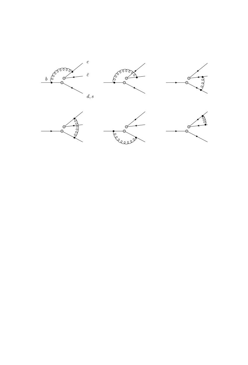
FIG. 1.: One-loop virtual corrections to $b\to c\bar{c}q$. Wave function renormalizations are not shown.

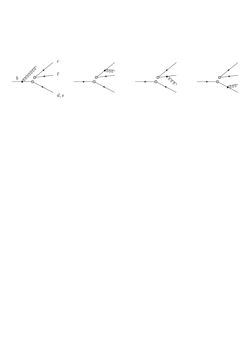
FIG. 2.: Real gluon corrections to $b\to c\bar{c}q$.

The NLO QCD corrections involve the one-loop virtual gluon correction to $b\to c\bar{c}[n]+q$ and the real gluon correction $b\to c\bar{c}[n]+q+g$, where the $c\bar{c}$ pair is projected on one of the states in (2). The corresponding diagrams are shown in Figs. 1 and 2 respectively. The decay rate into a quarkonium can be written as the sum of partial decay rates through one of the intermediate $c\bar{c}$ states $n$. At next-to-leading order the partial decay rates take the form

$$\Gamma[n] = \Gamma_{0}\,\Big{[}C_{[1,8]}^{2}f[n](\eta)\left(1+\delta_{P}[n]\right)$$ (16)

$$+\,\frac{\alpha_{s}(\mu)}{4\pi}\left(C_{[1]}^{2}g_{1}[n](\eta)+2C_{[1]}C_{[8]}g_{2}[n](\eta)+C_{[8]}^{2}g_{3}[n](\eta)\right)\Big{]}\,\langle{\cal O}^{H}[n]\rangle,$$

where

$$\Gamma_{0}=\frac{G_{F}^{2}|V_{bc}|^{2}m_{b}^{3}}{216\pi(2m_{c})},$$ (17)

and $\eta=4m_{c}^{2}/m_{b}^{2}$. The operators ${\cal O}^{H}[n]$ are defined as in Ref. [2]. The LO term is multiplied by $C_{[1]}^{2}$ if $n$ is a colour singlet state and by $C_{[8]}^{2}$ if $n$ is a colour octet state. We also used the fact that $|V_{cs}|^{2}+|V_{cd}|^{2}\approx 1$ to high accuracy. The functions $f[n]$ and $g_{i}[n]$ will be given later. The LO contribution is multiplied by a correction term $\delta_{P}[n]$ due to the penguin operators in (3). Likewise, we write the quarkonium energy distribution as

$$\frac{d\Gamma[n]}{dx} = \Gamma_{0}\,\Big{[}C_{[1,8]}^{2}f[n](\eta)\left(1+\delta_{P}[n]\right)\,\delta(1+\eta-x)$$ (19)

$$+\,\frac{\alpha_{s}(\mu)}{4\pi}\left(C_{[1]}^{2}g_{1}[n](\eta,x)+2C_{[1]}C_{[8]}g_{2}[n](\eta,x)+C_{[8]}^{2}g_{3}[n](\eta,x)\right)\Big{]}\,\langle{\cal O}^{H}[n]\rangle$$

where $x=2P\cdot p_{b}/m_{b}^{2}$. Note that to leading order in $\Lambda_{QCD}/m_{b}$ we do not distinguish the $b$ quark mass from the $B$ meson mass. To the order in the velocity expansion considered in this paper, we can also identify the momentum of the quarkonium with the momentum $P$ of the $c\bar{c}$ pair. (The kinematic effect of distinguishing the two is discussed in Ref. [14].) Hence $x$ can also be identified with $2E_{H}/M_{B}$, where $E_{H}$ is the quarkonium energy in the $B$ meson rest frame and $M_{B}$ the $B$ meson mass.

We now discuss which intermediate $c\bar{c}$ states should be taken into account for the production of a given quarkonium $H$.

$J/\psi$, $\psi^{\prime}$: At leading order in the velocity expansion the spin-triplet $S$-wave charmonium states are produced directly from a $c\bar{c}$ pair with the same quantum numbers, i.e. $n={}^{3}\!S_{1}^{(1)}$. At order $v^{4}$ relative to this colour singlet contribution, a $\psi$ can materialize through the colour octet $c\bar{c}$ states $n={}^{3}\!S_{1}^{(8)},{}^{1}\!S_{0}^{(8)},{}^{3}\!P_{J}^{(8)}$, where the subscript ‘$J$’ implies a sum over $J=0,1,2$. The suppression factor $v^{4}$ follows from the counting rules for the multipole transitions for soft gluons that convert the state $n$ into the $\psi$ meson [2]. The leading order colour singlet contribution is proportional to $C_{[1]}^{2}$, while the colour octet terms are proportional to $C_{[8]}^{2}$. Because the weak effective Hamiltonian favours the production of colour octet $c\bar{c}$ pairs by a large factor

$$C_{[8]}^{2}/C_{[1]}^{2}\approx 15,$$ (20)

the colour octet contributions must be included, since their suppression by $v^{4}\sim 1/15$ (for $J/\psi$) can easily be compensated. (The numbers serve only as order of magnitude estimates of the relative importance of the colour singlet and the colour octet contributions.) According to the velocity counting rules, there is a correction of order $v^{2}$ to the colour singlet contribution related to the derivative operator ${\cal P}_{1}({}^{3}\!S^{(1)})$ as defined in Ref. [2]. Because it is multiplied by the small coefficient $C_{[1]}^{2}$, and because we will find that the colour singlet contribution is indeed a small contribution to the total production cross section, we do not consider this additional correction in what follows. Similar derivative operators contribute to the colour octet channels. We do not take them into account, because we do not take into account other corrections of order $v^{6}$ with the large coefficient $C_{[8]}^{2}$. Hence, even after including the NLO correction in $\alpha_{s}$, there remains an uncertainty of order $v^{2}\sim 25\%$ in the theoretical prediction, assuming that the long-distance matrix elements were accurately known.

$\eta_{c}$: The same discussion applies to the spin-singlet state. The colour singlet contribution involves $n={}^{1}\!S_{0}^{(1)}$. At relative order $v^{4}$, $\eta_{c}$ can be produced through the colour octet $c\bar{c}$ states $n={}^{1}\!S_{0}^{(8)},{}^{3}\!S_{1}^{(8)},{}^{1}\!P_{1}^{(8)}$.

$\chi_{cJ}$: At leading order in the velocity expansion, both $n={}^{3}\!P_{J}^{(1)}$ and $n={}^{3}\!S_{1}^{(8)}$ contribute to the production of a the spin-triplet $P$-wave state [7]. Because the partial production rate through the ${}^{3}\!S_{1}^{(8)}$ state is already multiplied by the large coefficient $C_{[8]}^{2}$, it is not necessary to go to higher orders in the velocity expansion. Note that, because of the $V-A$ structure of the weak vertex, a $c\bar{c}$ pair cannot be produced in a ${}^{3}\!P_{0,2}$ angular momentum state at LO in $\alpha_{s}$.

$h_{c}$: The same discussion as for the $\chi_{cJ}$ states applies to the spin-singlet $P$-wave state. In this case we take into account $n={}^{1}\!P_{1}^{(1)}$ and $n={}^{1}\!S_{0}^{(8)}$ at NLO in $\alpha_{s}$. Owing to the $V-A$ structure of the weak vertex, a $c\bar{c}$ pair cannot be produced in a ${}^{1}\!P_{1}$ angular momentum state at LO in $\alpha_{s}$.

III Outline of the calculation

The Feynman diagrams shown in Figs. 1 and 2 are projected onto a colour and angular momentum state as specified in (2). The virtual corrections contain ultraviolet (UV) divergences, which can be absorbed into a renormalization of the operators ${\cal O}_{1,8}$ in the weak effective Hamiltonian (3). The virtual corrections contain infrared (IR) divergences, which cancel against IR divergences in the real corrections. In addition, the real corrections contain IR divergences due to the emission of soft gluons from the $c$ or $\bar{c}$ lines, which do not cancel with IR divergences in the virtual correction, if the $c\bar{c}$ pair is projected on a $P$-wave state. These IR divergences can be factorized and absorbed into a renormalization of the non-perturbative matrix elements $\langle{\cal O}^{H}[n]\rangle$. In the following we provide some details on the UV and IR regularization, which are specific of the present calculation. More details on the strategy of a next-to-leading order calculation can be found in Ref. [15], which deals with quarkonium decay and total quarkonium production cross sections in fixed-target collisions.

A UV regularization and the treatment of $\gamma_{5}$

The UV divergences are regulated dimensionally and the IR divergences are regulated with a gluon mass. The UV divergences in the diagrams of Fig. 1 cancel against the UV divergences in diagrams (not shown in the figure) with the insertion of the 1-loop counterterm for ${\cal O}_{1,8}$. We combine the diagram with its counterterm diagram before projecting on a particular $c\bar{c}$ state $n$, and before taking the 2-particle phase space integral. This has the advantages that it avoids extending the projection to $d$ dimensions and that the phase space integral can also be done in four dimensions.

The finite part of the virtual gluon correction depends on the prescription for handling $\gamma_{5}$ in $d$ dimensions. This has to be chosen consistently with the one used to define the operators ${\cal O}_{1,8}$ in Ref. [13]. The prescription consists of a definition of $\gamma_{5}$ and its anti-commutation property, together with a choice of ‘evanescent operators’. The evanescent operators are implicitly defined by specifying the order $\epsilon$ (where $d=4-2\epsilon$) terms of the following products of Dirac matrices:

$$\gamma_{\rho}\gamma_{\alpha}\Gamma_{\mu}\otimes\gamma_{\rho}\gamma_{\alpha}\Gamma_{\mu} = (16+4X_{R}\epsilon)\,\Gamma_{\mu}\otimes\Gamma_{\mu}+E_{X}$$ (21)

$$\Gamma_{\mu}\gamma_{\rho}\gamma_{\alpha}\otimes\gamma_{\alpha}\gamma_{\rho}\Gamma_{\mu} = (4+4Y_{R}\epsilon)\,\Gamma_{\mu}\otimes\Gamma_{\mu}+E_{Y}$$ (22)

$$\Gamma_{\mu}\otimes\gamma_{\rho}\gamma_{\alpha}\Gamma_{\mu}\gamma_{\alpha}\gamma_{\rho} = (4+4Z_{R}\epsilon)\,\Gamma_{\mu}\otimes\Gamma_{\mu}+E_{Z}.$$ (23)

(Here we defined $\Gamma_{\mu}=\gamma_{\mu}(1-\gamma_{5})$.) The renormalization conventions of Refs. [13, 16] correspond to:

$$\mbox{NDR scheme}: \quad X_{\rm NDR}=-1\qquad Y_{\rm NDR}=Z_{\rm NDR}=-2,$$ (24)

$$\mbox{HV scheme\hskip 2.84544pt}: \,\,\quad X_{\rm HV}=-1\qquad\,\,\,\,\,Y_{\rm HV}=Z_{\rm HV}=0.$$ (25)

In the HV scheme, vertex diagrams are treated differently in Ref. [13] and Ref. [16]. As a consequence, as already mentioned above, in the HV scheme one has to multiply the coefficients $C_{\pm}(\mu)$ defined in refs. [11, 13] by the factor $1-4\alpha_{s}(\mu)/(3\pi)$, while this factor is already included in the definition of Ref. [16]. We checked that our final result is identical in the NDR and HV schemes up to terms beyond NLO accuracy, if we use the expressions for $C_{\pm}(\mu)$ of Sect. II including the additional factor just mentioned in the HV scheme.

The coefficient functions quoted in Sect. II refer to a Fierz version of the weak Hamiltonian different from (3) and Fierz transformations do not commute with renormalization in general. If we use the standard Fierz version rather than the singlet-octet form quoted in (3), this interchanges $Y_{R}$ and $Z_{R}$ in the results quoted in Appendix A.3. However, since in both schemes we used one has $Y_{R}=Z_{R}$, either of the two Fierz versions can be used.

The NLO calculation for $n={}^{3}\!S_{1}^{(1)}$ has already been done in Ref. [10] in the HV scheme. We find that our result for the functions $g_{i}[{}^{3}\!S_{1}^{(1)}]$ defined in (16) and given in the Appendix agrees with the result of Ref. [10]. Nevertheless our result for the contribution of this channel to the decay rate, given by $C_{[1]}^{2}\,f[{}^{3}\!S_{1}^{(1)}](\eta)\,+\,$NLO terms, differs from the one given in Ref. [10], because the authors of Ref. [10] used the coefficient functions of Ref. [13], but did not correct them (or alternatively, the low energy matrix elements) by the factor $1-4\alpha_{s}(\mu)/(3\pi)$. As explained above with the conventions of Ref. [13] this additional factor is necessary in the HV scheme to obtain a scheme-independent result.

B IR regularization and NRQCD factorization

The real and virtual corrections individually have double-logarithmic IR divergences, which we regulate by a gluon mass. However, after adding all contributions to the partonic process $b\to c\bar{c}+X$, the IR divergences do not cancel completely. The remaining IR divergences are associated only with emission from the $c$ and $\bar{c}$ quark. This is a necessary (but not sufficient) requirement for their factorization into NRQCD matrix elements as discussed in detail in Ref. [2].

In addition to these IR divergences related to soft gluon emission, the last diagram in Fig. 1 exhibits the well-known Coulomb divergence, when the relative momentum of the $c$ and $\bar{c}$ is set to zero. We regularize this divergence by keeping the relative momentum finite in the integrals, which would otherwise give rise to the Coulomb singularity.

In order to extract the short-distance parts $\Gamma[m]$ (see (16)) of the partonic decay, we write

$$\Gamma(b\to c\bar{c}[n]+X)=\sum_{m}\Gamma[m]\,\langle{\cal O}^{\rm pert}[m]\rangle,$$ (26)

where $\langle{\cal O}^{\rm pert}[m]\rangle$ denotes the NRQCD matrix element for a perturbative $c\bar{c}$ pair in the state $n$. At NLO one has to calculate the left-hand side and $\langle{\cal O}^{\rm pert}[m]\rangle$ to NLO.

The diagrams that contribute the $\alpha_{s}$ correction to $\langle{\cal O}^{\rm pert}[m]\rangle$ are shown in Fig. 3. For the first diagram (together with its complex conjugate) we obtain

$$\langle{\cal O}^{\rm pert,1}[n]\rangle_{\rm A}=\langle{\cal O}^{\rm pert,0}[n]\rangle\cdot A[n]\,a_{s}\cdot\frac{2\pi^{2}}{v},$$ (27)

where $A[n]=C_{F}=4/3$, if $n$ is a colour singlet state, $A[n]=-1/(2N_{c})=-1/6$ if $n$ is a colour octet state and $v$ is the relative velocity of the two quarks. (The superscript ‘0’ refers to a matrix element at tree level, ‘1’ denotes a 1-loop contribution.) This renders the short-distance coefficients free of the Coulomb singularity.

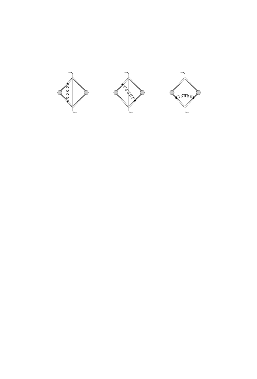
FIG. 3.: Perturbative corrections to the NRQCD operator matrix elements. A shaded circle denotes an insertion that specifies the angular momentum and colour of the $c\bar{c}$ pair. The vertical line implies that the diagram is ‘cut’. Symmetric diagrams are not shown.

The other two diagrams (called collectively ‘B’) together with their symmetry partners are UV and IR divergent. We define the NRQCD matrix elements in the $\overline{\rm MS}$ scheme and denote their renormalization scale by $\hat{\mu}$. The IR divergence is regulated with a gluon mass to be consistent with the IR regulator used for the evaluation of the partonic process on the left-hand side of (26). The result is (compare with the Appendix of Ref. [2] and with Ref. [15], where other IR regulators are used):

$$\langle{\cal O}^{\rm pert,1}_{1}({}^{3}\!S_{1})\rangle_{\rm B} = \frac{\alpha_{s}}{4\pi}\left(\ln\frac{\lambda^{2}}{\hat{\mu}^{2}}+\frac{1}{3}\right)\left(-48\right)\langle{\cal O}^{\rm pert,0}_{8}({}^{3}\!P_{0})\rangle/m_{c}^{2},$$ (28)

$$\langle{\cal O}^{\rm pert,1}_{8}({}^{3}\!S_{1})\rangle_{\rm B} = \frac{\alpha_{s}}{4\pi}\left(\ln\frac{\lambda^{2}}{\hat{\mu}^{2}}+\frac{1}{3}\right)\bigg{[}\left(-\frac{32}{3}\right)\langle{\cal O}^{\rm pert,0}_{1}({}^{3}\!P_{0})\rangle/m_{c}^{2}$$ (30)

$$+\,\left(-20\right)\langle{\cal O}^{\rm pert,0}_{8}({}^{3}\!P_{0})\rangle/m_{c}^{2}\bigg{]},$$

$$\langle{\cal O}^{\rm pert,1}_{1}({}^{1}\!S_{0})\rangle_{\rm B} = \frac{\alpha_{s}}{4\pi}\left(\ln\frac{\lambda^{2}}{\hat{\mu}^{2}}+\frac{1}{3}\right)\left(-\frac{16}{3}\right)\langle{\cal O}^{\rm pert,0}_{8}({}^{1}\!P_{1})\rangle/m_{c}^{2},$$ (31)

$$\langle{\cal O}^{\rm pert,1}_{8}({}^{1}\!S_{0})\rangle_{\rm B} = \frac{\alpha_{s}}{4\pi}\left(\ln\frac{\lambda^{2}}{\hat{\mu}^{2}}+\frac{1}{3}\right)\bigg{[}\left(-\frac{32}{27}\right)\langle{\cal O}^{\rm pert,0}_{1}({}^{1}\!P_{1})\rangle/m_{c}^{2}$$ (33)

$$+\,\left(-\frac{20}{9}\right)\langle{\cal O}^{\rm pert,0}_{8}({}^{1}\!P_{1})\rangle/m_{c}^{2}\bigg{]}.$$

($\lambda$ denotes the gluon mass.) Note that if one breaks up the ${}^{3}\!P$ term into terms with different $J$, one should replace

$$\langle{\cal O}^{\rm pert,0}_{1,8}({}^{3}\!P_{0})\rangle\to 1/9\,(\langle{\cal O}^{\rm pert,0}_{1,8}({}^{3}\!P_{0})\rangle+\langle{\cal O}^{\rm pert,0}_{1,8}({}^{3}\!P_{1})\rangle+\langle{\cal O}^{\rm pert,0}_{1,8}({}^{3}\!P_{2})\rangle).$$ (34)

Using these results and solving for $\Gamma[n]$ we find the IR finite short-distance coefficients for each $n$ collected in Appendix A.3.

C Difficulties with the colour singlet channels

The LO contributions to the colour singlet channels ${}^{1}\!S_{0}^{(1)}$, ${}^{3}\!S_{1}^{(1)}$ and ${}^{3}\!P_{1}^{(1)}$ are proportional to the small and strongly scale dependent coefficient $C_{[1]}^{2}(\mu)$. One would therefore expect the NLO contribution to be particularly important for these channels. However, the strict NLO calculation leads to a negative, and therefore meaningless decay rate into these channels and to the conclusion that a reliable result can only be obtained at next-to-next-to-leading order. This problem was already identified and discussed in Ref. [10]. (For the remainder of this section it is assumed that the reader has consulted Ref. [10] for more details.)

Consider the three next-to-leading order terms $g_{i}$ in (16). Despite its large coefficient $C_{[8]}^{2}$ the $g_{3}$-term, which comes only from a real correction, turns out to be numerically very small (see the tables in the following section). Both $g_{1}$ and $g_{2}$ (at $\mu=m_{b}$) are large and negative, and $g_{2}$ in particular, which comes with the larger coefficient $2C_{[1]}C_{[8]}$, drives the decay rate negative.

The authors of Ref. [10] suggested treating the decay process in a simultaneous expansion in $\alpha_{s}$ and $C_{[1]}/C_{[8]}$. This implies that one should add to the term of order $\alpha_{s}C_{[1]}C_{[8]}$ all terms of order $\alpha_{s}^{2}C_{[8]}^{2}$, because they also count as NLO in this rearranged expansion. On the other hand, the term $\alpha_{s}C_{[1]}^{2}$ (which involves $g_{1}$) should be neglected as being of higher order. The authors of Ref. [10] did not actually calculate all terms of order $\alpha_{s}^{2}C_{[8]}^{2}$, but estimated them by adding

$$\Gamma_{0}\,\langle{\cal O}^{H}[n]\rangle\left(\frac{\alpha_{s}(\mu)}{4\pi}\right)^{2}\,C_{[8]}^{2}\,\frac{g_{2}[n]^{2}}{f[n]}$$ (35)

to (16). This estimate can be motivated as follows: the virtual contribution to $g_{2}$ is given by the first four diagrams in Fig. 1 times the (complex conjugated) tree amplitude. All two-particle $[c\bar{c}]q$ cuts to the $\alpha_{s}^{2}C_{[8]}^{2}$ term are given by the square of the first four diagrams in Fig. 1. Hence, ignoring the real contribution, one may argue that $g_{2}[n]^{2}/f[n]$ is close (but not equal) to the two-particle contributions to the $\alpha_{s}^{2}C_{[8]}^{2}$ term.

In Ref. [17] the square of the 1-loop amplitude with a $[c\bar{c}]q$ final state is computed exactly and argued to provide a better estimate than the original one of Ref. [10], because one leaves out only real contributions to the coefficient of $\alpha_{s}^{2}C_{[8]}^{2}$, which are argued to be phase-space suppressed. However, we find that for the ${}^{3}\!P_{1}^{(1)}$ channel the virtual contributions alone are IR divergent. Therefore the real correction that cancels this divergence cannot be argued to be small. In our opinion this also calls into question the assumption that the real contributions are numerically small for the $S$-wave channels. For this reason we choose to follow with a minor modification the procedure of Ref. [10], which adds an IR finite term by construction, since $g_{2}$ is IR finite. The minor modification is the following: the third and fourth diagrams in Fig. 1 have imaginary parts, which contribute to the real part of the square of the amplitude (and hence to the coefficient of $\alpha_{s}^{2}C_{[8]}^{2}$). The remnants of these imaginary parts after multiplying the one-loop amplitude by the complex conjugate of the tree amplitude can easily be restored from the $\ln(1-\eta)$-term (and $\mbox{Li}_{2}(\eta)$-term in the case of ${}^{3}\!P_{1}^{(1)}$) in the results presented in Appendix A.3. If we call the restored imaginary part $\mbox{Im}\,g_{2}$, then we use (35), with $g_{2}^{2}$ replaced by $g_{2}^{2}+(\mbox{Im}\,g_{2})^{2}$.

We wish to emphasize two points: first, the discussed modifications of the colour singlet channels are certainly ad hoc and should be regarded with great caution. Second, the effect on the decay rate into a particular quarkonium state is not severely affected by this uncertainty, because it is dominated by colour octet contributions, whose short-distance coefficients can be computed reliably at NLO as we shall see.

In order to gain a numerical understanding of the importance of the various terms involved in the colour singlet channels, we consider in the following three computational schemes for the decay rate: (a) the (strict) NLO calculation; (b) the NLO calculation with the term (35) added, but without the $g_{1}$-term (‘improved’); (c) the same as (b), but with $g_{1}$ included (‘total’). For the $S$-wave colour singlet channels, (a) and (c) yield a negative rate. They are therefore meaningless. Option (b) yields a positive result of a magnitude similar to the result of Refs. [10, 17]. It may be considered as an order-of-magnitude estimate for the colour singlet contribution, but it may well be uncertain by 100%. For the ${}^{3}\!P_{1}^{(1)}$ channel all three options give negative partial rates. However, since this channel mixes with ${}^{3}\!S_{1}^{(8)}$ and only the sum of the two is physical, a negative partial rate is not unphysical by itself.

IV Results and Discussion

In this section we present our results for the branching fractions of $B$ decay into charmonium and moments of the quarkonium energy distributions in numerical form. The analytic expressions that enter (16) and (19) are collected in the appendices for reference.

A Branching ratios for $B$ decay into charmonium

1 General discussion of NLO corrections

We normalize our calculation to the theoretical expression for the inclusive semileptonic decay rate

$$\Gamma^{\rm th}_{\rm SL}=\frac{G_{F}^{2}|V_{bc}|^{2}m_{b}^{5}}{192\pi^{3}}\left(1-8z^{2}+8z^{6}-z^{8}-24z^{4}\ln z\right)\eta_{1}(z),$$ (36)

where $z=m_{c}/m_{b}$ and

$$\eta_{1}(z)=1-\frac{2\alpha_{s}(m_{b})}{3\pi}\left(\frac{3}{2}+\left(-\frac{31}{4}+\pi^{2}\right)\left(1-z\right)^{2}\right)$$ (37)

represents an excellent approximation [18] for the 1-loop QCD correction factor. (The complete analytic result can be found in Ref. [19].) For any particular quarkonium state $H$, we obtain the branching fraction in the form

$$\mbox{Br}\,(B\to H+X) = {\cal N}\,\sum_{n}\,\langle{\cal O}^{H}[n]\rangle\Big{[}C_{[1,8]}^{2}f[n](\eta)\left(1+\delta_{P}[n]\right)$$ (39)

$$+\,\frac{\alpha_{s}(\mu)}{4\pi}\left(C_{[1]}^{2}g_{1}[n](\eta)+2C_{[1]}C_{[8]}g_{2}[n](\eta)+C_{[8]}^{2}g_{3}[n](\eta)\right)\Big{]}.$$

The overall factor is given by

$${\cal N}=\mbox{Br}^{\rm exp}_{\rm SL}\,\frac{\Gamma_{0}}{\Gamma^{\rm th}_{\rm SL}}=3.0\cdot 10^{-2}\,{\rm GeV}^{-3},$$ (40)

where we used $\mbox{Br}^{\rm exp}_{\rm SL}=10.4\%$ and $\Gamma_{0}$ as given by (17). The charm and bottom pole masses are taken to be $1.5\,$GeV and $4.8\,$GeV, respectively. This yields $\eta=0.39$, which we use unless otherwise mentioned. The sensitivity of the charmonium production cross sections to the quark mass values will be discussed below.

We first examine the impact of the next-to-leading order correction and the dependence on the factorization scale $\mu$ for each intermediate $c\bar{c}$ state separately. We neglect the penguin contribution for this purpose. In Table I we show the branching fractions excluding the dimensionless normalization factor ${\cal N}\langle{\cal O}^{H}[n]\rangle$ for three values of $\mu$ at LO and at NLO. To evaluate the LO expression we also use the Wilson coefficients at LO and 1-loop running of the strong coupling with $\Lambda_{QCD}^{LO}$ such that $\alpha_{s}(M_{Z})=0.119$ both in LO and NLO. This is a large effect for the colour singlet channel, since $C_{[1]}(m_{b})=0.55$, $C_{[8]}(m_{b})=2.14$ (in the NDR scheme) but $C_{[1]}^{LO}(m_{b})=0.41$, $C_{[8]}^{LO}(m_{b})=2.19$.

$$\begin{array}[]{c|c|c|c|c|c|c}\hline\cr\hline\cr n&\vrule\lx@intercol\hfil\mbox{LO}\hfil\lx@intercol\vrule\lx@intercol&\vrule\lx@intercol\hfil\mbox{NLO}\hfil\lx@intercol\\ \hline\cr\mu/\mbox{GeV}&2.5&5&10&2.5&5&10\\ \hline\cr{}^{1}\!S_{0}^{(1)}&0.0453&0.201&0.407&-0.219&-0.426&-0.554\\ {}^{3}\!S_{1}^{(1)}&0.0269&0.119&0.242&-0.119&-0.250&-0.334\\ {}^{3}\!P_{0}^{(1)}&0&0&0&-0.660&-0.481&-0.377\\ {}^{3}\!P_{1}^{(1)}&0.0537&0.238&0.484&-0.654&-0.738&-0.794\\ {}^{3}\!P_{2}^{(1)}&0&0&0&-0.534&-0.389&-0.305\\ {}^{1}\!P_{1}^{(1)}&0&0&0&-1.02&-0.741&-0.58\\ \hline\cr{}^{1}\!S_{0}^{(8)}&8.72&8.01&7.51&12.6&11.1&10.2\\ {}^{3}\!S_{1}^{(8)}&5.18&4.75&4.46&7.70&6.80&6.18\\ {}^{3}\!P_{J}^{(8)}&31.1&28.5&26.8&38.3&34.5&31.7\\ {}^{1}\!P_{1}^{(8)}&0&0&0&-1.95&-1.53&-1.30\\ \hline\cr\hline\cr\end{array}\vspace*{0.2cm}$$

TABLE I.: Comparison of LO and NLO for the decay rate into a $c\bar{c}$ pair in state $n$ and the dependence on the factorization scale $\mu$. The dimensionless overall factor ${\cal N}\,\langle{\cal O}^{H}[n]\rangle$ is not included. Quark masses: $m_{b}=4.8\,$GeV, $m_{c}=1.5\,$GeV. Penguin contribution not included.

$$\begin{array}[]{c|c|c|c|c}\hline\cr\hline\cr n&\mu&{}^{1}\!S_{0}^{(1)}&{}^{3}\!S_{1}^{(1)}&{}^{3}\!P_{1}^{(1)}\\ \hline\cr&2.5&0.0453&0.0269&0.054\\ \mbox{LO}&5&0.201&0.119&0.238\\ &10&0.407&0.242&0.484\\ \hline\cr&2.5&-0.219&-0.119&-0.654\\ \mbox{NLO}&5&-0.426&-0.250&-0.738\\ &10&-0.554&-0.334&-0.794\\ \hline\cr&2.5&0.0951&0.034&-0.392\\ \mbox{`Impr'}&5&0.058&0.0259&-0.280\\ &10&0.0706&0.0402&-0.176\\ \hline\cr&2.5&0.0283&-0.0138&-0.455\\ \mbox{`Tot'}&5&-0.0984&-0.0862&-0.427\\ &10&-0.159&-0.124&-0.391\\ \hline\cr\hline\cr\end{array}\vspace*{0.2cm}$$

TABLE II.: The same quantity as in Table I for various treatments of the colour singlet channel (for which the LO short distance coefficient, i.e. $f[n]$, is non-vanishing). Penguin contribution not included.

We now observe that the colour singlet contributions are, as expected, enormously scale-dependent at LO. The NRQCD matrix element $\langle{\cal O}_{1}^{J/\psi}({}^{3}\!S_{1})\rangle$ is related to the radial wavefunction at the origin by $\langle{\cal O}_{1}^{J/\psi}({}^{3}\!S_{1})\rangle=9|R(0)|^{2}/(2\pi)$ up to corrections of order $v^{4}$. Using $\langle{\cal O}_{1}^{J/\psi}({}^{3}\!S_{1})\rangle=1.16\,$GeV³ [20], we obtain

$$\mbox{Br}\,(B\to J/\psi+X)=(0.09-0.84)\%\qquad\mbox{(colour singlet, LO)}$$ (41)

to be compared with the measured branching fraction $(0.80\pm 0.08)\%$ [3]. The LO prediction is uncertain by a factor of about 10 for all colour singlet channels, as can be seen from Table I. As also seen from this table, the scale uncertainty is reduced to a factor 2–3 at NLO. However, the NLO correction term renders the partial decay rates negative, as already mentioned in Section III C.

The situation can be somewhat improved by adding the estimate (35) for the order $\alpha_{s}^{2}$ NNLO term with the large coefficient $C_{[8]}^{2}$, while treating the $\alpha_{s}C_{[1]}^{2}$ term as formally of higher order in a double expansion in $\alpha_{s}$ and $C_{[1]}/C_{[8]}$ [10]. The addition of (35) also reduces the factorization scale dependence further, because it contains exactly the double logarithmic correction $\alpha_{s}^{2}C_{[8]}^{2}\ln^{2}(m_{b}^{2}/\mu^{2})$, which is required to cancel the large scale dependence of $C_{[1]}^{2}$ at leading order in $\alpha_{s}$. In Table II we display the result for the partial decay rates into the colour singlet channel, which is obtained in this way (denoted ‘Impr’ in the table) and for comparison again the LO and NLO result. The improvement can and should be done only for those colour singlet channels that have non-vanishing LO contributions. The last three rows of Table II show the results that are obtained if we add back the $g_{1}$ term in (39) to the improved treatment. The $\alpha_{s}C_{[1]}^{2}g_{1}$ term is sizeable and negative and therefore re-introduces a large scale dependence. The same improvement that is applied to the LO $C_{[1]}^{2}f$ term is necessary for the $g_{1}$ term, which would require going to order $\alpha_{s}^{3}C_{[8]}^{2}$. One may argue that unless this is done, it is preferable to leave the $g_{1}$ term out entirely. Therefore we shall use the ‘improved’ version (‘Impr’ in Table II) as our default option later. While the result is certainly not accurate, we believe that this is the best we can do to the colour singlet channel without making arbitrary modifications. We note that for $J/\psi$ this gives a colour singlet contribution to the branching fraction, which is close to the lower limit in (41) and also compatible with the estimates of Refs. [10, 17]. It seems safe to conclude that colour singlet production alone is not sufficient to explain the measured branching fraction.

The partial rates in the four relevant colour octet channels are shown in the lower part of Table I. In this case we find that the perturbative expansion is very well behaved. The NLO short-distance coefficients are larger by 20%–50% than the LO coefficients and the scale dependence is very moderate. The scale dependence is not reduced from LO to NLO. This is due to the fact that the LO coefficients depend only on the scale-insensitive $C_{[8]}$, while there are sizeable coefficients of the highly scale-dependent combinations $C_{[1]}C_{[8]}$ and $C_{[1]}^{2}$ at NLO. The numerical enhancement of the short-distance coefficients in the colour octet channels, which is evident from Table I, is sufficient to account for the measured $J/\psi$ branching fraction, as already noted in Refs. [8, 9]. The positive NLO correction reinforces this trend. Other $J/\psi$ production processes suggest that the long-distance parameters in the colour octet channels are of the order a few times $10^{-2}\,$GeV³. (This will be made more precise soon.) This leads to typical branching fractions of order $0.5\%$.

$$\begin{array}[]{c|c|c|c|c|c}\hline\cr\hline\cr n&f&\delta_{P}&g_{1}&g_{2}&g_{3}\\ \hline\cr{}^{3}\!S_{1}^{(1)}&0.661&-0.004&-20.5&-8.46+2.65\ln(m_{b}^{2}/\mu^{2})&0.162\\ {}^{3}\!S_{1}^{(8)}&0.992&-0.09&0.486&-6.35+1.98\ln(m_{b}^{2}/\mu^{2})&32.0-3.97\ln(m_{b}^{2}/\mu^{2})\\ {}^{1}\!S_{0}^{(8)}&1.67&0.009&0.556&-11.2+3.34\ln(m_{b}^{2}/\mu^{2})&50.2-6.68\ln(m_{b}^{2}/\mu^{2})\\ {}^{3}\!P_{J}^{(8)}&5.95&0.009&-129&-36.6+11.9\ln(m_{b}^{2}/\mu^{2})&121-23.8\ln(m_{b}^{2}/\mu^{2})\\ \hline\cr\hline\cr\end{array}$$

TABLE III.: Numerical values for the LO and NLO functions (NDR scheme) that enter the branching ratio $\mbox{Br}\,(B\to J/\psi+X)$ according to (39) for $m_{b}=4.8\,$GeV, $m_{c}=1.5\,$GeV. The estimate for the penguin correction $\delta_{P}$ is obtained with the parameters detailed in Appendix A.2. The table applies without modification to $\psi^{\prime}$.

$$\begin{array}[]{c|c|c|c|c|c}\hline\cr\hline\cr n&f&\delta_{P}&g_{1}&g_{2}&g_{3}\\ \hline\cr{}^{1}S_{0}^{(1)}&1.11&0.07&-28.6&-15.0+4.46\ln(m_{b}^{2}/\mu^{2})&0.185\\ {}^{1}S_{0}^{(8)}&1.67&0.009&0.556&-11.2+3.34\ln(m_{b}^{2}/\mu^{2})&50.2-6.68\ln(m_{b}^{2}/\mu^{2})\\ {}^{3}S_{1}^{(8)}&0.992&-0.09&0.486&-6.35+1.98\ln(m_{b}^{2}/\mu^{2})&32.0-3.97\ln(m_{b}^{2}/\mu^{2})\\ {}^{1}P_{1}^{(8)}&0&0&-28.2&0&-17.4\\ \hline\cr\hline\cr\end{array}$$

TABLE IV.: Numerical values for the LO and NLO functions (NDR scheme) that enter the branching ratio $\mbox{Br}\,(B\to\eta_{c}+X)$ according to (39) for $m_{b}=4.8\,$GeV, $m_{c}=1.5\,$GeV. The estimate for the penguin correction $\delta_{P}$ is obtained with the parameters detailed in Appendix A.2.

$$\begin{array}[]{c|c|c|c|c|c}\hline\cr\hline\cr n&f&\delta_{P}&g_{1}&g_{2}&g_{3}\\ \hline\cr{}^{3}P_{0}^{(1)}&0&0&0&0&-6.11\\ {}^{3}S_{1}^{(8)}&0.992&-0.09&0.486&-6.35+1.98\ln(m_{b}^{2}/\mu^{2})&32.0-3.97\ln(m_{b}^{2}/\mu^{2})\\ \hline\cr\hline\cr\end{array}$$

TABLE V.: Numerical values for the LO and NLO functions (NDR scheme) that enter the branching ratio $\mbox{Br}\,(B\to\chi_{c0}+X)$ according to (39) for $m_{b}=4.8\,$GeV, $m_{c}=1.5\,$GeV. The estimate for the penguin correction $\delta_{P}$ is obtained with the parameters detailed in Appendix A.2.

$$\begin{array}[]{c|c|c|c|c|c}\hline\cr\hline\cr n&f&\delta_{P}&g_{1}&g_{2}&g_{3}\\ \hline\cr{}^{3}P_{1}^{(1)}&1.32&0.07&-26.8&-16.3+5.29\ln(m_{b}^{2}/\mu^{2})&-4.04\\ {}^{3}S_{1}^{(8)}&0.992&-0.09&0.486&-6.35+1.98\ln(m_{b}^{2}/\mu^{2})&32.0-3.97\ln(m_{b}^{2}/\mu^{2})\\ \hline\cr\hline\cr\end{array}$$

TABLE VI.: Numerical values for the LO and NLO functions (NDR scheme) that enter the branching ratio $\mbox{Br}\,(B\to\chi_{c1}+X)$ according to (39) for $m_{b}=4.8\,$GeV, $m_{c}=1.5\,$GeV. The estimate for the penguin correction $\delta_{P}$ is obtained with the parameters detailed in Appendix A.2.

$$\begin{array}[]{c|c|c|c|c|c}\hline\cr\hline\cr n&f&\delta_{P}&g_{1}&g_{2}&g_{3}\\ \hline\cr{}^{3}P_{2}^{(1)}&0&0&0&0&-4.94\\ {}^{3}S_{1}^{(8)}&0.992&-0.09&0.486&-6.35+1.98\ln(m_{b}^{2}/\mu^{2})&32.0-3.97\ln(m_{b}^{2}/\mu^{2})\\ \hline\cr\hline\cr\end{array}$$

TABLE VII.: Numerical values for the LO and NLO functions (NDR scheme) that enter the branching ratio $\mbox{Br}\,(B\to\chi_{c2}+X)$ according to (39) for $m_{b}=4.8\,$GeV, $m_{c}=1.5\,$GeV. The estimate for the penguin correction $\delta_{P}$ is obtained with the parameters detailed in Appendix A.2.

$$\begin{array}[]{c|c|c|c|c|c}\hline\cr\hline\cr n&f&\delta_{P}&g_{1}&g_{2}&g_{3}\\ \hline\cr{}^{1}P_{1}^{(1)}&0&0&0&0&-9.41\\ {}^{1}S_{0}^{(8)}&1.67&0.009&0.556&-11.2+3.34\ln(m_{b}^{2}/\mu^{2})&50.2-6.68\ln(m_{b}^{2}/\mu^{2})\\ \hline\cr\hline\cr\end{array}$$

TABLE VIII.: Numerical values for the LO and NLO functions (NDR scheme) that enter the branching ratio $\mbox{Br}\,(B\to h_{c}+X)$ according to (39) for $m_{b}=4.8\,$GeV, $m_{c}=1.5\,$GeV. The estimate for the penguin correction $\delta_{P}$ is obtained with the parameters detailed in Appendix A.2.

For our standard value of the quark masses ($m_{b}=4.8\,$GeV, $m_{c}=1.5\,$GeV), the numerical values for the functions that enter (39) are given in Tables III–VIII for all of the six (known) charmonium states below the $D\bar{D}$ threshold. We keep the dependence on the factorization scale of the weak Hamiltonian $\mu$, but put the NRQCD factorization scale equal to $2m_{c}$. At the scale $m_{b}=4.8\,$GeV we also have $\alpha_{s}(m_{b})=0.22$ and $C_{[1]}(m_{b})=0.55$, $C_{[8]}(m_{b})=2.14$. The tables also include the penguin correction factor $\delta_{P}$.

We find that the dependence on the quark masses changes little when going from LO to NLO (for those $n$ for which the LO term is non-zero). The quark mass dependence is reasonably well estimated by that of the ratio

$$r=\frac{(1-4m_{c}^{2}/m_{b}^{2})^{2}}{m_{b}^{2}m_{c}f_{1}(m_{c}/m_{b})},$$ (42)

where $f_{1}(z)$ is the tree-level phase space factor in round brackets in (36) and the NRQCD matrix elements are assumed fixed. If we vary $m_{c}$ by $\pm 100\,$MeV and $m_{b}$ by $\pm 200\,$MeV around our ‘standard’ values and add the separate variations in square, we find a variation of $r$ of about 15% relative to the standard value. Taking into account the approximativeness of this estimate, we assign an overall normalization uncertainty of 20% due to quark masses.

2 $B\to\psi(nS)+X$

We now turn to a more specific discussion of $B$ decay into the spin-triplet $S$-wave states $J/\psi$ and $\psi^{\prime}$, denoted collectively by $\psi(nS)$ or just $\psi$. For quick reference we give the branching ratio in completely numerical form for $\mu=m_{b}=4.8\,$GeV and $m_{c}=1.5\,$GeV:

$$\mbox{Br}\,(B\to\psi(nS)+X) = \left\{\begin{array}[]{c}-0.741\\ 0.0754\\ -0.254\\ \end{array}\right\}10^{-2}\,\langle{\cal O}^{\psi}_{1}(^{3}\!S_{1})\rangle+0.195\langle{\cal O}^{\psi}_{8}(^{3}\!S_{1})\rangle$$ (47)

$$+\,0.342\left[\langle{\cal O}^{\psi}_{8}(^{1}\!S_{0})\rangle+\frac{3.10}{m_{c}^{2}}\,\langle{\cal O}^{\psi}_{8}(^{3}\!P_{0})\rangle\right].$$

The penguin correction is included. For the coefficient of the colour singlet operator we display the result obtained according to the procedures ‘NLO’, ‘Improved’ and ‘Total’ in Table II. As discussed earlier, we use the second entry (‘Improved’) in the following.

FIG. 4.: The $J/\psi$ branching fraction as a function of renormalization scale $\mu$ for various values of $M_{3.1}^{\psi}({}^{1}\!S_{1}^{(8)},{}^{3}\!P_{J}^{(8)})$ in $10^{-2}\,$GeV³. The horizontal band shows the CLEO measurement [3] and the dashed curve the colour singlet contribution alone.

The colour singlet matrix element is computed from the wave functions at the origin obtained with the Buchmüller-Tye potential as given in Ref. [20]:

$$\langle{\cal O}_{1}^{\psi}({}^{3}\!S_{1})\rangle=\frac{9|R(0)|^{2}}{2\pi}=\left\{\begin{array}[]{c}\,\,1.16\,\mbox{GeV}^{3}\qquad(J/\psi)\\ \!0.76\,\mbox{GeV}^{3}\qquad(\psi^{\prime})\end{array}\right.$$ (48)

The colour octet matrix element $\langle{\cal O}_{8}^{\psi}({}^{3}\!S_{1})\rangle$ is rather well determined by direct $\psi$ production at large transverse momentum in $p\bar{p}$ collisions [21, 22, 23]. We use the values [23]:

$$\langle{\cal O}_{8}^{\psi}({}^{3}\!S_{1})\rangle=\left\{\begin{array}[]{c}\,\,\,1.06\cdot 10^{-2}\,\mbox{GeV}^{3}\qquad(J/\psi)\\ \!0.44\cdot 10^{-2}\,\mbox{GeV}^{3}\qquad(\psi^{\prime})\end{array}\right.$$ (49)

There is an uncertainty of a factor 2 in each direction of the central value associated with these numbers. With the number quoted the ${}^{3}\!S_{1}^{(8)}$ channel contributes 0.21% to the $J/\psi$ branching fraction and 0.09% to the $\psi^{\prime}$ branching fraction. The other two colour octet matrix elements are not yet well determined. In Fig. 4 we show the $J/\psi$ branching fraction as a function of the renormalization scale $\mu$ for various values of $M_{3.1}^{\psi}({}^{1}\!S_{1}^{(8)},{}^{3}\!P_{J}^{(8)})$, where

$$M_{k}^{\psi}({}^{1}\!S_{1}^{(8)},{}^{3}\!P_{J}^{(8)})=\langle{\cal O}^{\psi}_{8}(^{1}\!S_{0})\rangle+\frac{k}{m_{c}^{2}}\,\langle{\cal O}^{\psi}_{8}(^{3}\!P_{0})\rangle.$$ (50)

With the other parameters fixed, the branching ratios $\mbox{Br}\,(B\to J/\psi+X)=(0.80\pm 0.08)\%$ and $\mbox{Br}\,(B\to\psi^{\prime}+X)=(0.34\pm 0.05)\%$ measured by CLEO are reproduced by

$$M_{3.1}^{\psi}({}^{1}\!S_{1}^{(8)},{}^{3}\!P_{J}^{(8)})=\left\{\begin{array}[]{c}\,\,\,1.5\cdot 10^{-2}\,\mbox{GeV}^{3}\qquad(J/\psi)\\ 0.6\cdot 10^{-2}\,\mbox{GeV}^{3}\qquad(\psi^{\prime}).\end{array}\right.$$ (51)

If we allow the colour singlet contribution to vary between zero and twice the value assumed above, include the above variation of $\langle{\cal O}_{8}^{\psi}({}^{3}\!S_{1})\rangle$ as well as the experimental error, and add all variations linearly, we obtain the allowed range

$$M_{3.1}^{\psi}({}^{1}\!S_{1}^{(8)},{}^{3}\!P_{J}^{(8)})=\left\{\begin{array}[]{c}\,\,\,(0.4-2.3)\cdot 10^{-2}\,\mbox{GeV}^{3}\qquad(J/\psi)\\ (0.0-1.0)\cdot 10^{-2}\,\mbox{GeV}^{3}\qquad(\psi^{\prime}).\end{array}\right.$$ (52)

It is interesting to compare the central values (51) and the upper limits with other determinations of the parameter $M_{k}^{\psi}({}^{1}\!S_{1}^{(8)},{}^{3}\!P_{J}^{(8)})$. The central values are about a factor 3 smaller than the central values obtained for $M_{3.5}^{\psi}({}^{1}\!S_{1}^{(8)},{}^{3}\!P_{J}^{(8)})$ from $\psi$ production at the Tevatron at moderate transverse momentum [22, 23]. As emphasized in Ref. [23] the Tevatron extraction is very sensitive to various effects that affect the transverse momentum distribution. Indeed, Refs. [24, 25] quote smaller values compatible with, or smaller than the central values above. The total production cross section in fixed target collisions probes $M_{7}^{\psi}({}^{1}\!S_{1}^{(8)},{}^{3}\!P_{J}^{(8)})$ (assuming the validity of NRQCD factorization, which may be controversial). Given that a different combination of matrix elements enters, the values obtained in Ref. [26] are certainly consistent with the above central value. In view of the uncertainties involved in charmonium production in hadron collisions, we believe that the above upper limit on $M_{3.1}^{\psi}({}^{1}\!S_{1}^{(8)},{}^{3}\!P_{J}^{(8)})$ is the most stringent one existing at present. We note that small values of $\langle{\cal O}^{\psi}_{8}(^{1}\!S_{0})\rangle$ and $\langle{\cal O}^{\psi}_{8}(^{3}\!P_{0})\rangle$ seem to be preferred by the non-observation of a significant colour octet contribution in the energy spectrum of inelastic $J/\psi$ photoproduction [27, 8, 28] (see, however, the discussion in Ref. [14]). We conclude that the measured $J/\psi$ and $\psi^{\prime}$ branching fractions can be accounted for with values of the NRQCD long-distance parameters consistent with previously available values.

3 $B\to\eta_{c}+X$

Presently, only an experimental upper bound $\mbox{Br}\,(B\to\eta_{c}+X)<0.9\%$ [3] exists on $\eta_{c}$ production. For the same choice of input parameters as above, we have

$$\mbox{Br}\,(B\to\eta_{c}+X) = \left\{\begin{array}[]{c}-1.19\\ 0.250\\ -0.210\\ \end{array}\right\}10^{-2}\,\langle{\cal O}^{\eta_{c}}_{1}(^{1}\!S_{0})\rangle+0.342\langle{\cal O}^{\eta_{c}}_{8}(^{1}\!S_{0})\rangle$$ (57)

$$+\,0.195\left[\langle{\cal O}^{\eta_{c}}_{8}(^{3}\!S_{1})\rangle-\frac{0.240}{m_{c}^{2}}\,\langle{\cal O}^{\eta_{c}}_{8}(^{1}\!P_{1})\rangle\right].$$

The LO term is enhanced by about 10% because of the penguin correction.

There is at present no information on the $\eta_{c}$ colour octet matrix elements from other $\eta_{c}$ production processes. The colour octet matrix elements are non-zero because soft gluon emission connects the colour octet $c\bar{c}$ state to the physical charmonium state. The soft gluon emission amplitude can be multipole expanded, supposing that the characteristic momentum of the emitted gluons is of order $m_{c}v^{2}$, smaller than the characteristic momentum $m_{c}v$ of the charm quarks in the charmonium rest frame. Up to corrections of order $v^{2}$, spin symmetry imposes relations between the $\eta_{c}$ and $J/\psi$ matrix elements. In addition to the familiar spin symmetry relation $\langle{\cal O}^{J/\psi}_{1}(^{3}\!S_{1})\rangle=3\,\langle{\cal O}^{\eta_{c}}_{1}(^{1}\!S_{0})\rangle$ for the colour singlet wave function, we find

$$\langle{\cal O}^{\eta_{c}}_{8}(^{1}\!S_{0})\rangle = \frac{1}{3}\,\langle{\cal O}^{J/\psi}_{8}(^{3}\!S_{1})\rangle,$$ (58)

$$\langle{\cal O}^{\eta_{c}}_{8}(^{3}\!S_{1})\rangle = \langle{\cal O}^{J/\psi}_{8}(^{1}\!S_{0})\rangle,$$ (59)

$$\langle{\cal O}^{\eta_{c}}_{8}(^{1}\!P_{1})\rangle = 3\,\langle{\cal O}^{J/\psi}_{8}(^{3}\!P_{0})\rangle.$$ (60)

Note that these relations are consistent with the renormalization group equations for the matrix elements that follow from (28). Since we do not know $\langle{\cal O}^{J/\psi}_{8}(^{1}\!S_{0})\rangle$ and $\langle{\cal O}^{J/\psi}_{8}(^{3}\!P_{0})\rangle$ separately, we assume that between one half and all of $M_{3.1}^{\psi}({}^{1}\!S_{1}^{(8)},{}^{3}\!P_{J}^{(8)})$ is due to $\langle{\cal O}^{J/\psi}_{8}(^{1}\!S_{0})\rangle$. With the central value from (51) this leads to the estimate

$$\mbox{Br}\,(B\to\eta_{c}+X)\approx(0.3-0.5)\%.$$ (61)

We emphasize that this estimate is crude and depends sensitively on the validity of the relations (58). This estimate is below the $J/\psi$ branching fraction, but with the increase in statistics since the previous analysis [3], a branching fraction in the above range may perhaps be reached with the CLEO detector.

4 $B\to\chi_{cJ}+X$

Colour octet effects in charmonium production were in fact considered for the first time for $\chi_{c}$ production in $B$ decay [7]. The authors showed that the observed $\chi_{c2}$ signal can be explained by the production of a $c\bar{c}[{}^{3}\!S_{1}^{(8)}]$ state followed by a soft dipole transition. (Recall that at LO in the colour singlet model, $\chi_{c0}$ and $\chi_{c2}$ are not produced.) The LO production through a $c\bar{c}[{}^{3}\!S_{1}^{(8)}]$ pair corresponds to the IR sensitive contribution at order $\alpha_{s}$ in the ordinary colour singlet channel. Our NLO calculation adds to those the ‘hard’ contributions at order $\alpha_{s}$ in the colour singlet and the colour octet channels. With $m_{b}=4.8\,$GeV, $m_{c}=1.5\,$GeV and $\mu=m_{b}$ as usual we obtain

$$\mbox{Br}\,(B\to\chi_{c0}+X) = \frac{-0.0148}{m_{c}^{2}}\,\langle{\cal O}^{\chi_{c0}}_{1}(^{3}\!P_{0})\rangle+0.195\,\langle{\cal O}^{\chi_{c0}}_{8}(^{3}\!S_{1})\rangle,$$ (62)

$$\mbox{Br}\,(B\to\chi_{c1}+X) = \left\{\begin{array}[]{c}-2.14\\ -0.783\\ -1.21\\ \end{array}\right\}\frac{10^{-2}}{m_{c}^{2}}\,\langle{\cal O}^{\chi_{c1}}_{1}(^{3}\!P_{1})\rangle+0.195\,\langle{\cal O}^{\chi_{c1}}_{8}(^{3}\!S_{1})\rangle,$$ (66)

$$\mbox{Br}\,(B\to\chi_{c2}+X) = \frac{-0.0120}{m_{c}^{2}}\,\langle{\cal O}^{\chi_{c2}}_{1}(^{3}\!P_{2})\rangle+0.195\,\langle{\cal O}^{\chi_{c2}}_{8}(^{3}\!S_{1})\rangle$$ (67)

to be compared with the measurements [3]

$$\mbox{Br}\,(B\to\chi_{c1}+X) = (0.37\pm 0.07)\%,$$ (68)

$$\mbox{Br}\,(B\to\chi_{c2}+X) = (0.25\pm 0.10)\%.$$ (69)

Owing to the spin symmetry relations, valid up to higher order corrections in $v^{2}$,

$$\langle{\cal O}^{\chi_{cJ}}_{1}(^{3}\!P_{J})\rangle = (2J+1)\,\langle{\cal O}^{\chi_{c0}}_{1}(^{3}\!P_{0})\rangle,$$ (70)

$$\langle{\cal O}^{\chi_{cJ}}_{8}(^{3}\!S_{1})\rangle = (2J+1)\,\langle{\cal O}^{\chi_{c0}}_{8}(^{3}\!S_{1})\rangle,$$ (71)

only two of the six above parameters are independent. The colour singlet contribution is always negative. However, since the two matrix elements involved mix under renormalization each short-distance coefficient depends on an arbitrary convention to separate the two contributions. (We used the $\overline{\rm MS}$ scheme.) Hence a negative partial rate is not unphysical.

Due to the near-proportionality of (66), (67), we find, however, that it is very difficult to reproduce the experimental result with a reasonable choice of matrix elements. With most reasonable choices one obtains a $\chi_{c2}$ production cross section larger than the cross section for $\chi_{c1}$. If we take the colour singlet matrix element from the Buchmüller-Tye potential model [20],

$$\langle{\cal O}^{\chi_{c0}}_{1}(^{3}\!P_{0})\rangle/m_{c}^{2}=4.8\cdot 10^{-2}\,\mbox{GeV}^{3},$$ (72)

and adjust

$$\langle{\cal O}^{\chi_{c0}}_{8}(^{3}\!S_{1})\rangle=(4.5-6.5)\cdot 10^{-3}\,\mbox{GeV}^{3}$$ (73)

to reproduce the measured $\chi_{c2}$ branching fraction, we obtain

$$\mbox{Br}\,(B\to\chi_{c1}+X)=(0.15-0.27)\%,$$ (74)

which is below the measurement. We conclude that the expansion in $\alpha_{s}$ is not well behaved enough for $P$-wave charmonium production in $B$ decay, at least to next-to-leading order, to arrive at quantitative relations. The problem is caused to a large extent by the fact that the leading order colour singlet contribution to $\chi_{c1}$ production, which would have been expected to enhance $\chi_{c1}$ production relative to $\chi_{c2}$ production, is turned negative (or very small) at NLO.

In addition, the colour singlet contributions are also negative for $\chi_{c0}$ and $\chi_{c2}$, which have no leading order contribution. This requires large cancellations between a negative colour singlet contribution and a positive colour octet contribution. These cancellations may be considered an artefact of the $\overline{\rm MS}$ factorization scheme, which appears unnatural from this point of view.

Because of this unsatisfactory situation, we find it difficult to predict the $\chi_{c0}$ branching fraction better than the naive expectation of one fifth of the $\chi_{c2}$ branching fraction. Note that we consider the prediction for the $\chi_{c1}$ state less reliable than for the $\chi_{c2}$ state, so that the range for the colour octet matrix element obtained in (73) may not be totally unreasonable.

5 $B\to h_{c}+X$

Finally, we consider the production of the ${}^{1}\!P_{1}$ state $h_{c}$, which will probably be difficult to measure. With the usual choice of parameters:

$$\mbox{Br}\,(B\to h_{c}+X) = \frac{-0.0228}{m_{c}^{2}}\,\langle{\cal O}^{h_{c}}_{1}(^{1}\!P_{1})\rangle+0.342\,\langle{\cal O}^{h_{c}}_{8}(^{1}\!S_{0})\rangle.$$ (75)

We use the spin symmetry relation $\langle{\cal O}^{h_{c}}_{1}(^{1}\!P_{1})\rangle=3\,\langle{\cal O}^{\chi_{c0}}_{1}(^{3}\!P_{0})\rangle$ for the derivative of the wave function at the origin (squared) and the spin symmetry relation

$$\langle{\cal O}^{h_{c}}_{8}(^{1}\!S_{0})\rangle=3\,\langle{\cal O}^{\chi_{c0}}_{8}(^{3}\!S_{1})\rangle$$ (76)

for the colour octet matrix element. With the value of the colour singlet matrix element as quoted above and the colour octet matrix element in the range (73) we obtain the estimate

$$\mbox{Br}\,(B\to h_{c}+X)\approx(0.13-0.34)\%.$$ (77)

The given range hinges on the estimate (76), which follows from the statistical factor 3 for the E1 ${}^{1}\!S_{0}\to{}^{1}\!P_{1}$ transition and another factor 3 for the final state with $J=1$, provided we assume a spin-independent overlap integral in terms of colour singlet and colour octet wave functions. Then taking into account the fact that the definition of $\langle{\cal O}^{\chi_{c0}}_{8}(^{3}\!S_{1})\rangle$ does not include an average over the three initial polarizations, we obtain the relative factor $9/3=3$. Note again that (76) is consistent with (28).

B Quarkonium momentum distributions

We briefly address quarkonium momentum distributions. We restrict ourselves to the $S$-wave states $J/\psi$ and $\psi^{\prime}$, first because data exist at present only for these states [3] and second, because the theoretical prediction appears to be most reliable for the $S$-wave states.

The energy distributions of the $c\bar{c}$ -pair in the partonic process $b\to c\bar{c}[n]+q+g$ are collected in Appendix B. The partonic energy/momentum distributions are distributions in the mathematical sense and cannot be used to predict the physical momentum spectrum. Two effects lead to a smearing of the partonic energy/momentum distribution:

(a) The $b$ quark has a residual motion in the $B$ meson and does not decay at rest. This leads to an energy smearing of order $\Lambda$, where $\Lambda$ is the QCD scale. For $B$ decay into charmonium this ‘Fermi motion’ effect has already been modelled in Ref. [29], and more recently in Ref. [30].

(b) The second effect is related to the fact that charmonium production through colour octet $c\bar{c}[n]$ states requires the emission of soft gluons with energy of order $m_{c}v^{2}\approx\Lambda$. The NRQCD matrix elements measure the probability for the transition $n\to\,\mbox{charmonium}$, but do not take into account the kinematic effect of the soft gluon emission, which becomes important near the upper endpoint of the charmonium momentum distribution [14]. Because the maximal $J/\psi$ momentum in $B$ decay is only about $2\,$GeV, this effect is expected to be at least as important as the $b$ quark motion, especially in view of the large fraction of colour octet production. No attempt has been made so far to take this effect into account in a realistic model for the spectrum. Both effects are also related to the fact that the phase space boundaries in the partonic calculation depend on the quark masses rather than the $B$ meson, $J/\psi$ and $K$ masses.

$$\begin{array}[]{c|c|c|c|c}\hline\cr\hline\cr\mbox{Moment}&\langle{\cal O}^{\psi}_{1}(^{3}\!S_{1})\rangle&\langle{\cal O}^{\psi}_{8}(^{3}\!S_{1})\rangle&\langle{\cal O}^{\psi}_{8}(^{1}\!S_{0})\rangle&\langle{\cal O}^{\psi}_{8}(^{3}\!P_{0})\rangle/m_{c}^{2}\\ \hline\cr 0&7.5\cdot 10^{-4}&2.0\cdot 10^{-1}&3.4\cdot 10^{-1}&1.06\\ \mbox{L1}&5.1\cdot 10^{-4}&1.9\cdot 10^{-1}&3.3\cdot 10^{-1}&9.8\cdot 10^{-1}\\ \mbox{L2}&3.3\cdot 10^{-4}&1.8\cdot 10^{-1}&3.2\cdot 10^{-1}&9.2\cdot 10^{-1}\\ \mbox{L3}&1.7\cdot 10^{-4}&1.7\cdot 10^{-1}&3.1\cdot 10^{-1}&8.7\cdot 10^{-1}\\ \hline\cr\mbox{S1}&2.4\cdot 10^{-4}&8.7\cdot 10^{-3}&1.4\cdot 10^{-2}&7.9\cdot 10^{-2}\\ \mbox{S2}&5.4\cdot 10^{-5}&1.6\cdot 10^{-3}&2.3\cdot 10^{-3}&1.6\cdot 10^{-2}\\ \mbox{S3}&2.4\cdot 10^{-5}&5.8\cdot 10^{-4}&7.5\cdot 10^{-4}&6.1\cdot 10^{-3}\\ \hline\cr\hline\cr\end{array}$$

TABLE IX.: Coefficients of NRQCD matrix elements in GeV^-3 for the moments of the $J/\psi$ momentum distribution. ‘Ln’ denotes the moment with the weight function $z^{n}$, ‘Sn’ the moment with the weight function $(1-z)^{n}$.

In this paper neither of the two effects will be modelled. One expects them to be suppressed by powers of $\Lambda_{QCD}/m_{b,c}$ and $v^{2}$ provided a smooth average of the momentum distribution (like the integration to the total width) is taken. We define

$$\mbox{Br}\,(\psi,W) \equiv \int\limits_{0}^{1}dz\,W(z)\,\frac{1}{\Gamma_{B}}\,\frac{d\Gamma(B\to\psi+X)}{dz}$$ (78)

$$= \sum_{n}{\cal N}\,\langle{\cal O}^{\psi}[n]\rangle\int\limits_{2\sqrt{\eta}}^{1+\eta}dx\,\frac{d\Gamma[n]}{dx}\,W\!\left(\frac{\sqrt{x^{2}-4\eta}}{1-\eta}\right),$$ (79)

where $z\equiv|\vec{p}_{\psi}|/|\vec{p}_{\psi,max}|$ and $\Gamma_{B}$ is the total $B$ decay rate. The variable $x$ is the energy fraction, defined together with $d\Gamma[n]/dx$ in (19). (The functions $g_{i}[n](\eta,x)$ that enter there can be found in Appendix B.) Finally $W(z)$ is a smooth weight on the momentum distribution.

In Table IX we give the coefficients in front of the NRQCD matrix elements in (78) for the weight functions $z^{n}$ (Ln) and $(1-z)^{n}$ (Sn) up to $n=3$. For $n=0$ we recover the inclusive branching fraction (47). The first weight function increasingly weights the endpoint region as $n$ increases. Therefore one cannot take $n$ large without enhancing higher order terms in the velocity expansion [14] not taken into account here. The second weight function weights the small-momentum tail. The moments decrease rapidly with $n$, because, as expected, the spectrum favours a large momentum of the $\psi$. The LO order and NLO virtual contributions do not contribute to the Sn moments. These moments are directly sensitive to hard gluon radiation.

The momentum spectrum measured by CLEO [3] is given in the CLEO rest frame rather than the $B$ rest frame. With the improved statistics that should be available now, it will be interesting to see whether one can obtain additional information on charmonium production by comparing averages of the momentum spectrum with the above predictions. For example, one may think of using the Sn moments to determine the parameters $\langle{\cal O}^{\psi}_{8}(^{1}\!S_{0})\rangle$ and $\langle{\cal O}^{\psi}_{8}(^{3}\!P_{0})\rangle$ separately.

C Comparison with exclusive two-body modes

It is interesting to compare qualitative features of the theoretical result for inclusive charmonium production with the sum of the most important exclusive two-body decay channels containing charmonium. We discuss only $J/\psi$ because only limited experimental information exists for the other charmonium states.

There exist only two two-body modes of any importance. Their branching fractions are measured to be [31]

$$\mbox{Br}\,(B\to J/\psi+K) = \left\{\begin{array}[]{c}(0.099\pm 0.010)\%\\ (0.089\pm 0.012)\%,\end{array}\right.$$ (82)

$$\mbox{Br}\,(B\to J/\psi+K^{*}) = \left\{\begin{array}[]{c}(0.147\pm 0.027)\%\\ (0.135\pm 0.018)\%,\end{array}\right.$$ (85)

where the upper line in both (82) and (85) refers to $B^{\pm}$ and the lower one to $B^{0}$. The combined branching fraction of about 0.25% is far below the inclusive branching fraction of $0.80\pm 0.08\%$. The existence of a large fraction of three-body modes is also confirmed by the broad energy distribution measured by CLEO [3].

There is no clear association of the colour singlet contribution with the inclusive branching fraction with the above two-body modes. A colour singlet $c\bar{c}$ pair can radiate a hard gluon and end up as a three-body mode. Likewise, the soft gluon that is necessarily emitted from a $c\bar{c}$ pair in a colour octet state can be re-absorbed by the light quarks and combine to the kaon. This process depends on the spectator light quark in the $B$ meson and would therefore seem to violate the factorization hypothesis of the NRQCD approach. However, factorization requires only that such spectator dependence cancels out to first approximation (in $\Lambda_{QCD}/m_{c,b}$) in the average over all decay modes.

Nevertheless it is natural to expect that a $c\bar{c}$ pair in a colour octet state finds itself more often hadronizing in a multi-body decay than a colour singlet $c\bar{c}$ pair and therefore we consider the observation of a large fraction of multi-body decays as supporting evidence for the colour octet picture. The fact that the sum of the two two-body modes above is larger than the (poorly predicted) inclusive colour singlet branching fraction of approximately 0.1% suggests that the NLO calculation underestimates this contribution. (Another possibility is that some fraction of the large colour octet partial rate does in fact end up in two-body modes.)

The large fraction of three body decays is significant in another respect. The NRQCD approach assumes ‘local parton-hadron duality’, which is often discussed in connection with the inclusive non-leptonic decays of $B$ mesons. A crucial consequence of ‘local parton-hadron duality’ is that the effect of colour reconnections to the spectator quarks are small (power-suppressed) even though colour reconnections must occur in every single decay. The same assumption underlies the NRQCD factorization approach to inclusive charmonium production. The assumption is usually justified by the presence of a large energy release into the final state and many decay modes to be averaged over. Since the energy release in decays into charmonium is not particularly large, the existence of a sufficient fraction of decays with additional pions suggests that the total decay rate provides enough averaging for an approximate cancellation of non-factorizable effects.

V Conclusion

We presented an analysis of inclusive $B$ decay into the known charmonium states at next-to-leading order in the strong coupling and accounting for the most important colour singlet and colour octet production mechanisms. We find that radiative corrections make the colour singlet contributions negative, an effect already observed in Ref. [10] for the colour singlet contribution to $J/\psi$ production and explained by the suppression of colour singlet production at leading order due to the particular structure of the weak effective Hamiltonian. The problem is particularly serious for $\chi_{c1}$ production. As a consequence, the appealing theoretical pattern for $\chi_{cJ}$ production at leading order [7] becomes obscured quantitatively at next-to-leading order, although the qualitative requirement of an additional colour octet component is not put into question. In general, we find it difficult to make a quantitative prediction for any of the four $P$-wave states.

The situation is more satisfactory for $S$-wave production, and in particular for $J/\psi$ production, for which we confirm the earlier conclusion that the colour singlet contribution is about a factor 5–10 below the observed production rate. The next-to-leading order corrections to the colour octet channels computed in this paper are positive and of order 20%–50%. Assuming that these channels make up for the missing contribution, we adjust a certain combination of NRQCD matrix elements to reproduce the experimental branching fraction. The value for the matrix element is somewhat smaller than, but within errors compatible with the magnitude suggested by other quarkonium production processes. Since the $\alpha_{s}$ expansion appears to be well-behaved for $J/\psi$ production, we obtain the sharpest upper bound to date on a combination of $\langle{\cal O}^{\psi}_{8}(^{1}\!S_{0})\rangle$ and $\langle{\cal O}^{\psi}_{8}(^{3}\!P_{0})\rangle/m_{c}^{2}$, even when we assume that there are no other production mechanisms. In principle, with more accurate data appearing, weights on the $J/\psi$ momentum distribution can also be used to determine $\langle{\cal O}^{\psi}_{8}(^{1}\!S_{0})\rangle$ and $\langle{\cal O}^{\psi}_{8}(^{3}\!P_{0})\rangle/m_{c}^{2}$ individually, which has so far proven to be difficult, even combining information from other $J/\psi$ production processes.

Acknowledgements. We thank Gerhard Buchalla and Marco Ciuchini for helpful discussions on the renormalization of the weak effective Hamiltonian in the HV scheme. We thank Ben Grinstein for his interest in this work and Tom Ferguson and Giancarlo Moneti for their effort in explaining the data on $J/\psi$ momentum distributions to us. This work was supported in part by the EU Fourth Framework Programme ‘Training and Mobility of Researchers’, Network ‘Quantum Chromodynamics and the Deep Structure of Elementary Particles’, contract FMRX-CT98-0194 (DG 12 - MIHT) and by the DOE grant DOE-ER-40682-145.

Appendix A. Short-distance coefficients for integrated decay widths

We collect the expressions that enter the integrated partial rates (16) in this appendix. Recall $\eta=4m_{c}^{2}/m_{b}^{2}$. The scale $\mu$ denotes the factorization scale at which the coefficients $C_{[1,8]}$ are evaluated. We distinguish from it the renormalization scale $\hat{\mu}$ of the NRQCD matrix element $\langle{\cal O}^{H}[n]\rangle$.

A.1. Lowest order functions

The lowest order function $f[n](\eta)$ vanishes for $n={}^{3}\!P_{0}^{(1)},\,^{3}\!P_{2}^{(1)},\,^{1}\!P_{1}^{(1)}$ and ${}^{1}\!P_{1}^{(8)}$. The non-vanishing ones are:

$$f[^{3}\!S_{1}^{(1)}](\eta) = (1-\eta)^{2}(1+2\eta),$$ (A.86)

$$f[^{1}\!S_{0}^{(1)}](\eta) = 3\,(1-\eta)^{2},$$ (A.87)

$$f[^{3}\!P_{1}^{(1)}](\eta) = 2\,(1-\eta)^{2}(1+2\eta),$$ (A.88)

$$f[^{3}\!S_{1}^{(8)}](\eta) = \frac{3}{2}\,(1-\eta)^{2}(1+2\eta),$$ (A.89)

$$f[^{1}\!S_{0}^{(8)}](\eta) = \frac{9}{2}\,(1-\eta)^{2},$$ (A.90)

$$f[^{3}\!P_{J}^{(8)}](\eta) = 9\,(1-\eta)^{2}(1+2\eta).$$ (A.91)

A.2. The penguin correction

We consider only the contribution where a decay through a QCD penguin operator ${\cal O}_{3-6}$ interferes with the decay amplitude through a current-current operator. Since the penguin operators have small coefficient functions, it is sufficient to evaluate the penguin contributions in lowest orders in $\alpha_{s}$. The double penguin contribution is negligible in size. Since $f[n](\eta)=0$ for $n={}^{3}\!P_{0}^{(1)},\,^{3}\!P_{2}^{(1)},\,^{1}\!P_{1}^{(1)},\,^{1}\!P_{1}^{(8)}$, the penguin contribution also vanishes in leading order for these $n$. For the other intermediate states, we find

$$\delta_{P}[^{3}\!S_{1}^{(1)}]=2\,\frac{3(C_{3}+C_{5})+C_{4}+C_{6}}{C_{[1]}}\approx-0.004,$$ (A.92)

$$\delta_{P}[^{1}\!S_{0}^{(1)}]=\delta_{P}[^{3}\!P_{1}^{(1)}]=2\,\frac{3(C_{3}-C_{5})+C_{4}-C_{6}}{C_{[1]}}\approx 0.07,$$ (A.93)

$$\delta_{P}[^{3}\!S_{1}^{(8)}]=4\,\frac{C_{4}+C_{6}}{C_{[8]}}\approx-0.09,$$ (A.94)

$$\delta_{P}[^{1}\!S_{0}^{(8)}]=\delta_{P}[^{3}\!P_{J}^{(8)}]=4\,\frac{C_{4}-C_{6}}{C_{[8]}}\approx 0.009.$$ (A.95)

Here we used unitarity of the Cabibbo-Kobayashi-Maskawa (CKM) matrix to relate the CKM factor of the penguin contribution to the CKM factor of the current-current operator contribution (up to a negligible error $\mbox{Re}\,(V_{cb}^{*}V_{cs}/(V_{tb}^{*}V_{ts}))=-1$). For the numerical estimate we have used the leading logarithmic approximation for the Wilson coefficients at the scale $m_{b}=4.8\,$GeV and with $\Lambda_{QCD}^{LO}$ adjusted to reproduce $\alpha_{s}(m_{Z})$ which gives $\Lambda_{QCD}^{LO}=93\,$MeV (for 5 flavours). This implies $C_{[1]}(m_{b})=0.41$, $C_{[8]}(m_{b})=2.19$, $C_{3}(m_{b})=0.010$, $C_{4}(m_{b})=-0.024$, $C_{5}(m_{b})=0.007$ and $C_{6}(m_{b})=-0.028$.

A.3. Next-to-leading order functions

The next-to-leading order functions depend on the scheme-dependent constants $X_{R}$, $Y_{R}$ and $Z_{R}$. Their values in the NDR and HV scheme are given in section III A.

A.3.1. ${}^{3}\!S_{1}^{(1)}$

$$g_{1}[^{3}\!S_{1}^{(1)}](\eta) = \frac{4}{3}\Bigg{\{}(-1)\,(1-\eta)^{2}(1+2\eta)\bigg{[}8\,\mbox{Li}_{2}(\eta)+4\ln(1-\eta)\ln\eta-4Z_{R}+\frac{4\pi^{2}}{3}\bigg{]}$$ (A.98)

$$-\,4\,\eta(1+\eta)\,(1-2\eta)\,\ln\eta-2\,(1-\eta)^{2}\,(5+4\eta)\,\ln(1-\eta)$$

$$-\,(1-\eta)\,(1-2\eta)\,(3+5\eta)\Bigg{\}}.$$

$$g_{2}[^{3}\!S_{1}^{(1)}](\eta) = \frac{4}{3}\Bigg{\{}(1-\eta)^{2}(1+2\eta)\left[3\ln\frac{m_{b}^{2}}{\mu^{2}}+Y_{R}-X_{R}\right]$$ (A.101)

$$-\,\frac{(1-\eta)(34+23\eta-51\eta^{2}+16\eta^{3})}{2(2-\eta)}+\frac{2(1-\eta)^{3}(3-\eta^{2})}{(2-\eta)^{2}}\ln(1-\eta)$$

$$-\,\frac{(26-19\eta+4\eta^{2})\eta^{2}}{2-\eta}\ln\eta-\frac{8(1-\eta)^{3}\eta}{2-\eta}\ln 2\Bigg{\}}.$$

$$g_{3}[^{3}\!S_{1}^{(1)}](\eta) = \frac{4}{27}\,(1-\eta)\,(1+37\eta-8\eta^{2})-\frac{8\,(1-6\eta)}{9}\,\ln\eta.$$ (A.102)

A.3.2. ${}^{1}\!S_{0}^{(1)}$

$$g_{1}[^{1}\!S_{0}^{(1)}](\eta) = (-4)\,(1-\eta)^{2}\bigg{[}8\,\mbox{Li}_{2}(\eta)+4\ln(1-\eta)\ln\eta-4Z_{R}+\frac{4\pi^{2}}{3}\bigg{]}$$ (A.104)

$$-\,16\,\eta(1-\eta)\,\ln\eta+\frac{8\,(1-\eta)^{2}\,(2-5\eta)}{\eta}\,\ln(1-\eta)+20\,(1-\eta)^{2}.$$

$$g_{2}[^{1}\!S_{0}^{(1)}](\eta) = 4(1-\eta)^{2}\left[3\ln\frac{m_{b}^{2}}{\mu^{2}}+Y_{R}-X_{R}\right]+4\eta^{2}\,\ln\eta$$ (A.106)

$$-\,\frac{2(1-\eta)(34-53\eta+17\eta^{2})}{2-\eta}+\frac{8\,(1-\eta)^{3}(3-\eta)}{(2-\eta)^{2}}\,\ln(1-\eta).$$

$$g_{3}[^{1}\!S_{0}^{(1)}](\eta) = \frac{4}{9}\,\left((-1)\,(1-\eta)\,(11-7\eta+2\eta^{2})-6\ln\eta\right).$$ (A.107)

A.3.3. ${}^{3}\!P_{0}^{(1)}$

$$g_{1}[^{3}\!P_{0}^{(1)}](\eta) = 0.$$ (A.108)

$$g_{2}[^{3}\!P_{0}^{(1)}](\eta) = 0.$$ (A.109)

$$g_{3}[^{3}\!P_{0}^{(1)}](\eta) = \frac{16}{9}\,(1-\eta)^{2}\,(1+2\eta)\,\left[-\ln\frac{\hat{\mu}^{2}}{4m_{c}^{2}}+2\ln(1-\eta)\right]$$ (A.111)

$$-\,\frac{8}{9}\,(1-12\eta^{2}+8\eta^{3})\,\ln\eta-\frac{4}{9}\,(1-\eta)\,(25-13\eta-18\eta^{2}).$$

A.3.4. ${}^{3}\!P_{1}^{(1)}$

$$g_{1}[^{3}\!P_{1}^{(1)}](\eta) = \left(-\frac{8}{3}\right)\,(1-\eta)^{2}\,(1+2\eta)\bigg{[}8\,\mbox{Li}_{2}(\eta)+4\ln(1-\eta)\ln\eta-4Z_{R}+\frac{4\pi^{2}}{3}\bigg{]}$$ (A.114)

$$-\,\frac{32}{3}\,\eta\,(1+\eta)\,(1-2\eta)\,\ln\eta-\frac{16}{3}\,(1-\eta)^{2}\,(5+4\eta)\,\ln(1-\eta)$$

$$+\,\frac{8}{3}\,(1-\eta)\,(5+9\eta-6\eta^{2}).$$

$$g_{2}[^{3}\!P_{1}^{(1)}](\eta) = \frac{8}{3}\,(1-\eta)^{2}(1+2\eta)\left(3\ln\frac{m_{b}^{2}}{\mu^{2}}+Y_{R}-X_{R}\right)$$ (A.119)

$$+\,\frac{64}{3}\,\eta^{2}\Bigg{(}-\mbox{Li}_{2}\Bigg{(}\frac{1-\eta}{2-\eta}\Bigg{)}+\mbox{Li}_{2}\Bigg{(}\frac{2(1-\eta)}{2-\eta}\Bigg{)}-2\mbox{Li}_{2}(\eta)-\ln 2\,\ln(2-\eta)+\ln 2\,\ln\eta$$

$$-\,\ln\eta\,\ln(1-\eta)+\frac{\pi^{2}}{3}\Bigg{)}+\frac{16(1-\eta)\,(3+8\eta^{2}-10\eta^{3}+3\eta^{4})}{3(2-\eta)^{2}}\,\ln(1-\eta)$$

$$-\,\frac{8\eta^{2}\,(48-96\eta+59\eta^{2}-12\eta^{3})}{3(2-\eta)^{2}}\,\ln\eta-\frac{32(1-\eta)\,\eta\,(4-21\eta+17\eta^{2}-4\eta^{3})}{3(2-\eta)^{2}}\,\ln 2$$

$$-\,\frac{4(1-\eta)\,(34+23\eta-3\eta^{2}-8\eta^{3})}{3(2-\eta)}.$$

$$g_{3}[^{3}\!P_{1}^{(1)}](\eta) = \frac{16}{9}\,(1-\eta)^{2}\,(1+2\eta)\,\left[-\ln\frac{\hat{\mu}^{2}}{4m_{c}^{2}}+2\ln(1-\eta)\right]$$ (A.121)

$$-\,\frac{16}{9}\,(1-2\eta)\,(1+2\eta-2\eta^{2})\,\ln\eta-\frac{8}{27}\,(1-\eta)\,(13+37\eta-56\eta^{2}).$$

A.3.5. ${}^{3}\!P_{2}^{(1)}$

$$g_{1}[^{3}\!P_{2}^{(1)}](\eta) = 0.$$ (A.122)

$$g_{2}[^{3}\!P_{2}^{(1)}](\eta) = 0.$$ (A.123)

$$g_{3}[^{3}\!P_{2}^{(1)}](\eta) = \frac{16}{9}\,(1-\eta)^{2}\,(1+2\eta)\,\left[-\ln\frac{\hat{\mu}^{2}}{4m_{c}^{2}}+2\ln(1-\eta)\right]$$ (A.125)

$$-\,\frac{16}{45}\,(1-30\eta^{2}+20\eta^{3})\,\ln\eta-\frac{8}{45}\,(1-\eta)\,(27+31\eta-76\eta^{2}).$$

A.3.6. ${}^{1}\!P_{1}^{(1)}$

$$g_{1}[^{1}\!P_{1}^{(1)}](\eta) = 0.$$ (A.126)

$$g_{2}[^{1}\!P_{1}^{(1)}](\eta) = 0.$$ (A.127)

$$g_{3}[^{1}\!P_{1}^{(1)}](\eta) = \frac{16}{3}\,(1-\eta)^{2}\,\left[-\ln\frac{\hat{\mu}^{2}}{4m_{c}^{2}}+2\ln(1-\eta)\right]$$ (A.129)

$$-\,\frac{8}{9}\,(1-6\eta+12\eta^{2})\,\ln\eta-\frac{4}{27}\,(1-\eta)\,(119-85\eta+8\eta^{2}).$$

A.3.7. ${}^{3}\!S_{1}^{(8)}$

$$g_{1}[^{3}\!S_{1}^{(8)}](\eta) = -\frac{8\,(1-6\eta)}{3}\,\ln\eta+\frac{4}{9}\,(1-\eta)\,(1+37\eta-8\eta^{2}).$$ (A.130)

$$g_{2}[^{3}\!S_{1}^{(8)}](\eta) = (1-\eta)^{2}(1+2\eta)\left(3\ln\frac{m_{b}^{2}}{\mu^{2}}+Y_{R}-X_{R}\right)$$ (A.133)

$$+\,\frac{2(1-\eta)^{3}(3-\eta^{2})}{(2-\eta)^{2}}\,\ln(1-\eta)-\Bigg{(}\frac{4(1-\eta)^{2}\eta^{2}}{2-\eta}+11\eta^{2}\Bigg{)}\,\ln\eta-\frac{8(1-\eta)^{3}\eta}{2-\eta}\,\ln 2$$

$$-\frac{(1-\eta)(34+23\eta-51\eta^{2}+16\eta^{3})}{2(2-\eta)}.$$

$$g_{3}[^{3}\!S_{1}^{(8)}](\eta) = \frac{3}{2}\,(1-\eta)^{2}\,(1+2\eta)\Bigg{(}-4\ln\frac{m_{b}^{2}}{\mu^{2}}+\frac{4}{3}X_{R}+\frac{14}{3}Y_{R}$$ (A.140)

$$-\,\frac{2}{3}Z_{R}-3\ln^{2}(2-\eta)+6\ln(1-\eta)\,\ln(2-\eta)\Bigg{)}$$

$$+\,(1-\eta)\,(1+2\eta)\Bigg{(}(29+7\eta)\,\mbox{Li}_{2}(\eta)-(7+29\eta)\,\frac{\pi^{2}}{6}+9\,(1+\eta)\,\mbox{Li}_{2}\Bigg{(}\frac{1-\eta}{2-\eta}\Bigg{)}$$

$$-\,18\,\mbox{Li}_{2}\Bigg{(}\frac{2(1-\eta)}{2-\eta}\Bigg{)}+18\,\ln 2\,\ln(2-\eta)-18\,\ln 2\,\ln\eta+2\,(5+4\eta)\,\ln\eta\,\ln(1-\eta)\Bigg{)}$$

$$-\,\frac{(1-\eta)^{2}(110+188\eta-291\eta^{2}+83\eta^{3})}{(2-\eta)^{2}}\,\ln(1-\eta)$$

$$+\,\frac{34+547\eta-1062\eta^{2}+1158\eta^{3}-426\eta^{4}}{6(2-\eta)}\,\ln\eta-\frac{(1-\eta)^{2}(18+83\eta-74\eta^{2})}{2-\eta}\,\ln 2$$

$$+\,\frac{(1-\eta)\,(5294+5779\eta-14795\eta^{2}+5228\eta^{3})}{36(2-\eta)}.$$

A.3.8. ${}^{1}\!S_{0}^{(8)}$

$$g_{1}[^{1}\!S_{0}^{(8)}](\eta) = -8\ln\eta-\frac{4}{3}\,(1-\eta)(11-7\eta+2\eta^{2}).$$ (A.141)

$$g_{2}[^{1}\!S_{0}^{(8)}](\eta) = 3(1-\eta)^{2}\left(3\ln\frac{m_{b}^{2}}{\mu^{2}}+Y_{R}-X_{R}\right)+\frac{6\,(3-\eta)(1-\eta)^{3}}{(2-\eta)^{2}}\,\ln(1-\eta)$$ (A.143)

$$+\,3\eta^{2}\ln\eta-\frac{3(1-\eta)(34-53\eta+17\eta^{2})}{2(2-\eta)}.$$

$$g_{3}[^{1}\!S_{0}^{(8)}](\eta) = \frac{9}{2}\,(1-\eta)^{2}\Bigg{(}-4\ln\frac{m_{b}^{2}}{\mu^{2}}+\frac{4}{3}X_{R}+\frac{14}{3}Y_{R}-\frac{2}{3}Z_{R}$$ (A.149)

$$-\,3\ln^{2}(2-\eta)+6\ln(1-\eta)\,\ln(2-\eta)-6\,\ln 2\Bigg{)}$$

$$+\,3\,(1-\eta)\Bigg{(}(29+7\eta)\,\mbox{Li}_{2}(\eta)-(7+29\eta)\,\frac{\pi^{2}}{6}+9\,(1+\eta)\,\mbox{Li}_{2}\Bigg{(}\frac{1-\eta}{2-\eta}\Bigg{)}$$

$$-\,18\,\mbox{Li}_{2}\Bigg{(}\frac{2(1-\eta)}{2-\eta}\Bigg{)}+18\,\ln 2\,\ln(2-\eta)-18\,\ln 2\,\ln\eta+2\,(5+4\eta)\,\ln\eta\,\ln(1-\eta)\Bigg{)}$$

$$-\,\frac{3(1-\eta)^{2}(4+106\eta-113\eta^{2}+33\eta^{3})}{(2-\eta)^{2}\,\eta}\,\ln(1-\eta)$$

$$+\,\frac{17-48\eta+90\eta^{2}}{2}\,\ln\eta+\frac{(1-\eta)\,(4478-6221\eta+2077\eta^{2}+20\eta^{3})}{12(2-\eta)}.$$

A.3.9. ${}^{3}\!P_{J}^{(8)}$

We have summed over $J=0,1,2$.

$$g_{1}[^{3}\!P_{J}^{(8)}](\eta) = (1-\eta)^{2}(1+2\eta)\Big{[}(-48)\,\ln\frac{\hat{\mu}^{2}}{4m_{c}^{2}}+96\,\ln(1-\eta)\Big{]}$$ (A.151)

$$-\,24\,(1-12\eta^{2}+8\eta^{3})\ln\eta-4(1-\eta)\,(35+41\eta-94\eta^{2}).$$

$$g_{2}[^{3}\!P_{J}^{(8)}](\eta) = 6(1-\eta)^{2}(1+2\eta)\left(3\ln\frac{m_{b}^{2}}{\mu^{2}}+Y_{R}-X_{R}\right)$$ (A.156)

$$+\,48\eta^{2}\Bigg{(}-\mbox{Li}_{2}\Bigg{(}\frac{1-\eta}{2-\eta}\Bigg{)}+\mbox{Li}_{2}\Bigg{(}\frac{2(1-\eta)}{2-\eta}\Bigg{)}-2\mbox{Li}_{2}(\eta)-\ln 2\,\ln(2-\eta)+\ln 2\,\ln\eta$$

$$-\,\ln\eta\,\ln(1-\eta)+\frac{\pi^{2}}{3}\Bigg{)}+\frac{12(1-\eta)\,(3+8\eta^{2}-10\eta^{3}+3\eta^{4})}{(2-\eta)^{2}}\,\ln(1-\eta)$$

$$-\,\frac{6\eta^{2}\,(48-96\eta+59\eta^{2}-12\eta^{3})}{(2-\eta)^{2}}\,\ln\eta-\frac{24(1-\eta)\,\eta\,(4-21\eta+17\eta^{2}-4\eta^{3})}{(2-\eta)^{2}}\,\ln 2$$

$$-\,\frac{3(1-\eta)\,(34+23\eta-3\eta^{2}-8\eta^{3})}{2-\eta}.$$

$$g_{3}[^{3}\!P_{J}^{(8)}](\eta) = (1-\eta)^{2}\,(1+2\eta)\,(-30)\,\ln\frac{\hat{\mu}^{2}}{4m_{c}^{2}}$$ (A.166)

$$+\,9\,(1-\eta)^{2}\,(1+2\eta)\Bigg{(}-4\ln\frac{m_{b}^{2}}{\mu^{2}}+\frac{4}{3}X_{R}+\frac{14}{3}Y_{R}-\frac{2}{3}Z_{R}-3\ln^{2}(2-\eta)$$

$$+\,6\ln(1-\eta)\,\ln(2-\eta)\Bigg{)}-12\,(3-4\eta)\,(3+7\eta)\Bigg{(}\mbox{Li}_{2}\Bigg{(}\frac{2(1-\eta)}{2-\eta}\Bigg{)}-\ln 2\,\ln(2-\eta)$$

$$+\,\ln 2\,\ln\eta\Bigg{)}+6\,(29+36\eta-91\eta^{2}-14\eta^{3})\,\mbox{Li}_{2}(\eta)$$

$$+\,6\,(9+18\eta-29\eta^{2}-18\eta^{3})\,\mbox{Li}_{2}\Bigg{(}\frac{1-\eta}{2-\eta}\Bigg{)}-(7+36\eta-25\eta^{2}-58\eta^{3})\,\pi^{2}$$

$$+\,12\,(5+9\eta-16\eta^{2}-8\eta^{3})\,\ln\eta\,\ln(1-\eta)$$

$$-\,\frac{30(1-\eta)(14+6\eta-69\eta^{2}+58\eta^{3}-13\eta^{4})}{(2-\eta)^{2}}\,\ln(1-\eta)$$

$$+\,\frac{3(4-68\eta-159\eta^{2}+632\eta^{3}-466\eta^{4}+106\eta^{5})}{(2-\eta)^{2}}\,\ln\eta$$

$$-\,\frac{6(1-\eta)(36+112\eta-399\eta^{2}+269\eta^{3}-58\eta^{4})}{(2-\eta)^{2}}\,\ln 2$$

$$+\,\frac{(1-\eta)(1078+851\eta-3757\eta^{2}+1402\eta^{3})}{2(2-\eta)}.$$

A.3.10. ${}^{1}\!P_{1}^{(8)}$

$$g_{1}[^{1}\!P_{1}^{(8)}](\eta) = 16\,(1-\eta)^{2}\,\left[-\ln\frac{\hat{\mu}^{2}}{4m_{c}^{2}}+2\ln(1-\eta)\right]$$ (A.168)

$$-\,\frac{8}{3}\,(1-6\eta+12\eta^{2})\,\ln\eta-\frac{4}{9}\,(1-\eta)\,(119-85\eta+8\eta^{2}).$$

$$g_{2}[^{1}\!P_{1}^{(8)}](\eta) = 0.$$ (A.169)

$$g_{3}[^{1}\!P_{1}^{(8)}](\eta) = 10\,(1-\eta)^{2}\,\left[-\ln\frac{\hat{\mu}^{2}}{4m_{c}^{2}}+2\ln(1-\eta)\right]$$ (A.171)

$$-\,\frac{2}{3}\,(7-15\eta+30\eta^{2})\,\ln\eta-\frac{1}{9}\,(1-\eta)\,(347-244\eta+29\eta^{2}).$$

Appendix B. Short-distance coefficients for energy distributions

At leading order in $\alpha_{s}$ the energy of the quarkonium is fixed. A non-trivial energy distribution is generated by gluon emission at NLO. The functions $g_{i}[n](\eta,x)$, where $x$ is the quarkonium energy fraction as defined in the text, can be expressed in the form

$$g_{i}[n](\eta,x)=g_{i}[n](\eta)\,\delta(1+\eta-x)+[g_{i,real}[n](\eta,x)]_{+},$$ (B.1)

where $g_{i}[n](\eta)$ is the corresponding function for the total integrated decay rate, given in Appendix A.3. The ‘plus-distribution’ is defined by

$$\int\limits_{2\sqrt{\eta}}^{1+\eta}dx\,\left[f(x)\right]_{+}\,t(x)=\int\limits_{2\sqrt{\eta}}^{1+\eta}dx\,f(x)\,(t(x)-t(1+\eta))$$ (B.2)

for a test function $t$. We also introduce

$$\rho=\sqrt{x^{2}-4\eta}.$$ (B.3)

The kinematic limits on $x$ are $2\sqrt{\eta}<x<1+\eta$. In the following we give the energy distribution functions $g_{i,real}[n](\eta,x)$.

B.1. ${}^{3}\!S_{1}^{(1)}$

$$g_{1,real}[^{3}\!S_{1}^{(1)}](x,\eta) = \frac{4}{3}\Bigg{(}-\frac{7(1+\eta-2\eta^{2})}{1+\eta-x}-(3-2\eta)\Bigg{)}\rho$$ (B.5)

$$+\frac{4}{3}\Bigg{(}\frac{4(1-\eta)^{2}(1+2\eta)}{1+\eta-x}+2(3+5\eta-2\eta^{2}-x-2\eta x)\Bigg{)}\ln\frac{2-x+\rho}{2-x-\rho}.$$

$$g_{2,real}[^{3}\!S_{1}^{(1)}](x,\eta) = -\frac{8}{3}(1-2\eta)\rho+\frac{8}{3}(1-3\eta-x)\ln\frac{2-x+\rho}{2-x-\rho}$$ (B.7)

$$+\frac{32}{3}\,\eta^{2}\ln\frac{2\eta-x-\rho}{2\eta-x+\rho}.$$

$$g_{3,real}[^{3}\!S_{1}^{(1)}](x,\eta) = \frac{4}{3}\,(2-x)\rho+\frac{16}{3}\,x(1+\eta-x)\ln\frac{2\eta-x-\rho}{2\eta-x+\rho}.$$ (B.8)

B.2. ${}^{1}\!S_{0}^{(1)}$

$$g_{1,real}[^{1}\!S_{0}^{(1)}](x,\eta) = \left(-\frac{28(1-\eta)}{1+\eta-x}-12\right)\,\rho$$ (B.10)

$$+\,\left(\frac{16\,(1-\eta)^{2}}{1+\eta-x}+8(3-\eta-x)\right)\ln\frac{2-x+\rho}{2-x-\rho}.$$

$$g_{2,real}[^{1}\!S_{0}^{(1)}](x,\eta) = -8\,\rho+8(1+\eta-x)\,\ln\frac{2-x+\rho}{2-x-\rho}.$$ (B.11)

$$g_{3,real}[^{1}\!S_{0}^{(1)}](x,\eta) = (-4)\,(6+8\eta-7x)\,\rho+16\,(1+\eta-x)\,(x-2\eta)\,\ln\frac{2\eta-x-\rho}{2\eta-x+\rho}.$$ (B.12)

B.3. ${}^{3}\!P_{0}^{(1)}$

$$g_{1,real}[^{3}\!P_{0}^{(1)}](x,\eta) = 0.$$ (B.13)

$$g_{2,real}[^{3}\!P_{0}^{(1)}](x,\eta) = 0.$$ (B.14)

$$g_{3,real}[^{3}\!P_{0}^{(1)}](x,\eta) = \frac{8}{9}\left(\frac{4(1-\eta)\,(1+2\eta)}{1+\eta-x}-\frac{1}{2}\,(26-40\eta+11x)\right)\rho$$ (B.16)

$$+\frac{16}{3}\left(2\eta^{2}+x-\eta x-x^{2}\right)\ln\frac{2\eta-x-\rho}{2\eta-x+\rho}.$$

B.4. ${}^{3}\!P_{1}^{(1)}$

$$g_{1,real}[^{3}\!P_{1}^{(1)}](x,\eta) = \left(-\frac{8}{3}\right)\left(\frac{7(1-\eta)(1+2\eta)}{1+\eta-x}+3-2\eta\right)\,\rho$$ (B.18)

$$+\frac{16}{3}\left(\frac{2(1-\eta)^{2}(1+2\eta)}{1+\eta-x}+3+5\eta-2\eta^{2}-x-2\eta x\right)\ln\frac{2-x+\rho}{2-x-\rho}.$$

$$g_{2,real}[^{3}\!P_{1}^{(1)}](x,\eta) = \frac{16}{3}\left(\frac{4\eta^{2}}{1+\eta-x}-(1-2\eta)\right)\,\rho$$ (B.21)

$$+\frac{16}{3}\left(\frac{4\eta^{2}}{1+\eta-x}+1-3\eta-x\right)\ln\frac{2-x+\rho}{2-x-\rho}$$

$$+\frac{32}{3}\left(-\frac{2\eta^{2}}{1+\eta-x}+3\eta^{2}\right)\ln\frac{2\eta-x-\rho}{2\eta-x+\rho}.$$

$$g_{3,real}[^{3}\!P_{1}^{(1)}](x,\eta) = \frac{8}{9}\left(\frac{4(1-\eta)(1+2\eta)}{1+\eta-x}-(16+34\eta-23x)\right)\rho$$ (B.23)

$$-\frac{16}{3}\left(3\eta+7\eta^{2}-2x-6\eta x+2x^{2}\right)\ln\frac{2\eta-x-\rho}{2\eta-x+\rho}.$$

B.5. ${}^{3}\!P_{2}^{(1)}$

$$g_{1,real}[^{3}\!P_{2}^{(1)}](x,\eta) = 0.$$ (B.24)

$$g_{2,real}[^{3}\!P_{2}^{(1)}](x,\eta) = 0.$$ (B.25)

$$g_{3,real}[^{3}\!P_{2}^{(1)}](x,\eta) = \frac{8}{9}\left(\frac{4(1-\eta)(1+2\eta)}{1+\eta-x}-(4-2\eta+x)\right)\rho$$ (B.27)

$$+\,\frac{16}{15}\left(3\eta-5\eta^{2}+2x-2\eta x-2x^{2}\right)\ln\frac{2\eta-x-\rho}{2\eta-x+\rho}.$$

B.6. ${}^{1}\!P_{1}^{(1)}$

$$g_{1,real}[^{1}\!P_{1}^{(1)}](x,\eta) = 0.$$ (B.28)

$$g_{2,real}[^{1}\!P_{1}^{(1)}](x,\eta) = 0.$$ (B.29)

$$g_{3,real}[^{1}\!P_{1}^{(1)}](x,\eta) = \frac{4}{3}\left(\frac{8\,(1-\eta)}{1+\eta-x}-(14+x)\right)\rho$$ (B.31)

$$-\,\frac{16}{3}\,(2\eta-x-\eta x+x^{2})\,\ln\frac{2\eta-x-\rho}{2\eta-x+\rho}.$$

B.7. ${}^{3}\!S_{1}^{(8)}$

$$g_{1,real}[^{3}\!S_{1}^{(8)}](x,\eta) = 4(2-x)\,\rho+16x(1+\eta-x)\,\ln\frac{2\eta-x-\rho}{2\eta-x+\rho}.$$ (B.32)

$$g_{2,real}[^{3}\!S_{1}^{(8)}](x,\eta) = -2\left(1-2\eta\right)\,\rho+2\left(1-3\eta-x\right)\ln\frac{2-x+\rho}{2-x-\rho}$$ (B.34)

$$+\,8\eta^{2}\,\ln\frac{2\eta-x-\rho}{2\eta-x+\rho}.$$

$$g_{3,real}[^{3}\!S_{1}^{(8)}](x,\eta) = \left(-\frac{32(1-\eta)(1+2\eta)}{1+\eta-x}+39+68\eta-\frac{77x}{2}\right)\,\rho$$ (B.37)

$$+\,\Bigg{(}-\frac{2(1-\eta)(1+2\eta)(5+4\eta)}{1+\eta-x}+17+5\eta-8\eta^{2}-9x-8\eta x\Bigg{)}\ln\frac{2-x+\rho}{2-x-\rho}$$

$$+\,\Bigg{(}\frac{18(1-\eta)(1+2\eta)}{1+\eta-x}-18+18\eta+92\eta^{2}+10x-26\eta x-10x^{2}\Bigg{)}\ln\frac{2\eta-x-\rho}{2\eta-x+\rho}.$$

B.8. ${}^{1}\!S_{0}^{(8)}$

$$g_{1,real}[^{1}\!S_{0}^{(8)}](x,\eta) = -12\left(6+8\eta-7x\right)\,\rho-48(1+\eta-x)(2\eta-x)\,\ln\frac{2\eta-x-\rho}{2\eta-x+\rho}.$$ (B.38)

$$g_{2,real}[^{1}\!S_{0}^{(8)}](x,\eta) = -6\rho+6(1+\eta-x)\,\ln\frac{2-x+\rho}{2-x-\rho}.$$ (B.39)

$$g_{3,real}[^{1}\!S_{0}^{(8)}](x,\eta) = \left(-\frac{96(1-\eta)}{1+\eta-x}-51-60\eta+\frac{105x}{2}\right)\,\rho$$ (B.42)

$$+\left(-\frac{6(1-\eta)(5+4\eta)}{1+\eta-x}+51+3\eta-27x\right)\ln\frac{2-x+\rho}{2-x-\rho}$$

$$+\left(\frac{54(1-\eta)}{1+\eta-x}-54-6\eta-60\eta^{2}+30x+90\eta x-30x^{2}\right)\ln\frac{2\eta-x-\rho}{2\eta-x+\rho}.$$

B.9. ${}^{3}\!P_{J}^{(8)}$

We have summed over $J=0,1,2$.

$$g_{1,real}[^{3}\!P_{J}^{(8)}](x,\eta) = \left(\frac{96(1-\eta)(1+2\eta)}{1+\eta-x}-12(18+16\eta-13x)\right)\,\rho$$ (B.44)

$$+\,48\left(-2\eta-8\eta^{2}+3x+5\eta x-3x^{2}\right)\ln\frac{2\eta-x-\rho}{2\eta-x+\rho}.$$

$$g_{2,real}[^{3}\!P_{J}^{(8)}](x,\eta) = \left(\frac{48\eta^{2}}{1+\eta-x}-12(1-2\eta)\right)\,\rho$$ (B.47)

$$+\left(\frac{48\eta^{2}}{1+\eta-x}+12(1-3\eta-x)\right)\ln\frac{2-x+\rho}{2-x-\rho}$$

$$+\left(-\frac{48\eta^{2}}{1+\eta-x}+72\eta^{2}\right)\ln\frac{2\eta-x-\rho}{2\eta-x+\rho}.$$

$$g_{3,real}[^{3}\!P_{J}^{(8)}](x,\eta) = \left(-\frac{12(11+11\eta-32\eta^{2})}{1+\eta-x}-24(5-12\eta+x)\right)\rho$$ (B.50)

$$+\left(-\frac{12(5+9\eta-16\eta^{2}-8\eta^{3})}{1+\eta-x}+6(17-4\eta-8\eta^{2}-9x-8\eta x\right)\ln\frac{2-x+\rho}{2-x-\rho}$$

$$+\left(\frac{12(3-4\eta)(3+7\eta)}{1+\eta-x}-6(18-8\eta-71\eta^{2}-24x+2\eta x+24x^{2})\right)\ln\frac{2\eta-x-\rho}{2\eta-x+\rho}.$$

B.10. ${}^{1}\!P_{1}^{(8)}$

$$g_{1,real}[^{1}\!P_{1}^{(8)}](x,\eta) = \left(\frac{32(1-\eta)}{1+\eta-x}-4(14+x)\right)\,\rho$$ (B.52)

$$-\,16\left(2\eta-x-\eta x+x^{2}\right)\ln\frac{2\eta-x-\rho}{2\eta-x+\rho}.$$

$$g_{2,real}[^{1}\!P_{1}^{(8)}](x,\eta) = 0.$$ (B.53)

$$g_{3,real}[^{1}\!P_{1}^{(8)}](x,\eta) = \left(\frac{20(1-\eta)}{1+\eta-x}-(62+36\eta-29x)\right)\rho$$ (B.55)

$$-\,4\left(14\eta+9\eta^{2}-7x-16\eta x+7x^{2}\right)\ln\frac{2\eta-x-\rho}{2\eta-x+\rho}.$$

REFERENCES

• [1]
• [2] G.T. Bodwin, E. Braaten and G.P. Lepage, Phys. Rev. D51, 1125 (1995) [Erratum: ibid. D55, 5853 (1997)].
• [3] R. Balest et al. (CLEO Collaboration), Phys. Rev. D52, 2661 (1995).
• [4] T.A. De Grand and D. Toussaint, Phys. Lett. B89, 256 (1980).
• [5] M.B. Wise, Phys. Lett. B89, 229 (1980).
• [6] J.H. Kühn, S. Nussinov and R. Rückl, Z. Phys. C5, 117 (1980).
• [7] G.T. Bodwin, E. Braaten, T.C. Yuan and G.P. Lepage, Phys. Rev. D46, 3703 (1992).
• [8] P. Ko, J. Lee and H.S. Song, Phys. Rev. D53, 1409 (1996); ibid. D54, 4312 (1996).
• [9] S. Fleming, O.F. Hernández, I. Maksymyk and H. Nadeau, Phys. Rev. D55, 4098 (1997).
• [10] L. Bergström and P. Ernström, Phys. Lett. B328, 153 (1994).
• [11] G. Buchalla, A.J. Buras and M.E. Lautenbacher, Rev. Mod. Phys. 68, 1125 (1996).
• [12] G. Altarelli, G. Curci, G. Martinelli and S. Petrarca, Nucl. Phys. B187, 461 (1981).
• [13] A.J. Buras and P.H. Weisz, Nucl. Phys. B333, 66 (1990).
• [14] M. Beneke, I.Z. Rothstein and M.B. Wise, Phys. Lett. B408, 373 (1997).
• [15] A. Petrelli et al., Nucl. Phys. B514, 245 (1998).
• [16] M. Ciuchini, E. Franco, G. Martinelli and L. Reina, Nucl. Phys. B415, 403 (1994).
• [17] J.M. Soares and T. Torma, Phys. Rev. D56, 1632 (1997).
• [18] C.S. Kim and A.D. Martin, Phys. Lett. B225, 186 (1989).
• [19] Y. Nir, Phys.Lett. B221, 184 (1989).
• [20] E. Eichten and C. Quigg, Phys. Rev. D52, 1726 (1995).
• [21] E. Braaten and S. Fleming, Phys. Rev. Lett. 74, 3327 (1995).
• [22] P. Cho and A.K. Leibovich, Phys. Rev. D53, 150 (1996); ibid. D53, 6203 (1996).
• [23] M. Beneke and M. Krämer, Phys. Rev. D55, 5269 (1997).
• [24] B. Cano-Coloma and M.A. Sanchis-Lozano, Nucl. Phys. B508, 753 (1997).
• [25] B.A. Kniehl and G. Kramer, [hep-ph/9803256].
• [26] M. Beneke and I.Z. Rothstein, Phys. Rev. D54, 2005 (1996); ibid. D54, 7082(E) (1996).
• [27] M. Cacciari and M. Krämer, Phys. Rev. Lett. 76, 4128 (1996).
• [28] M. Beneke, M. Krämer and M. Vänttinen, Phys. Rev. D57, 4258 (1998).
• [29] V. Barger, W.Y. Keung, J.P. Leveille and R.J.N. Phillips, Phys. Rev. D24, 2016 (1981).
• [30] W.F. Palmer, E.A. Paschos and P.H. Soldan, Phys. Rev. D56, 5794 (1997).
• [31] Particle Data Group, C. Caso et al., Eur. Phys. J. C3, 1 (1998).