Non-Equilibrium HTL Resummation

Abstract

We present an extension of the HTL resummation technique to non-equilibrium situations, starting from the real time formalism in the Keldysh representation. As an example we calculate the HTL photon self energy, from which we derive the resummed photon propagator. This propagator is applied to the computation of the interaction rate of a hard electron in a non-equilibrium QED plasma. In particular we show the absence of of pinch singularities in these quantities. Finally we show that the Ward identities relating the HTL electron self energy to the HTL electron-photon vertex hold as in equilibrium.

I Introduction

Perturbative QCD at finite temperature and density can be used to describe properties of an equilibrated quark-gluon plasma (QGP). However, using only bare propagators and vertices infrared divergent and gauge dependent result are obtained. These problems can be partly avoided by using the hard thermal loop (HTL) resummation technique [2]. In this way consistent results, which are complete to leading order in the coupling constant and gauge independent, are found. At the same time the infrared behavior is improved by the presence of effective masses in the HTL propagators. This method has been applied to various quantities of the QGP, such as damping rates of quarks and gluons, energy loss of energetic partons, thermalization times, viscosity, and photon and dilepton production [3].

The HTL method has been derived within the imaginary time formalism, which is restricted to equilibrium situations. However, in relativistic heavy ion collisions the formation of a pre-equilibrium parton gas has to be expected. Indeed it is not clear whether a complete thermal and chemical equilibrium will be reached in the evolution of the fireball at all [4]. Therefore it is desirable to extend the HTL resummation technique to non-equilibrium. For this purpose we have to start from the real time formalism (RTF) [5]. Similar investigations have been performed by Baier et al. [6].

In the RTF formalism propagators are given by $2\times 2$-matrices [7]. For example the scalar propagator reads

$$D(K) = \left(\begin{array}[]{cc}\frac{1}{K^{2}-m^{2}+i\epsilon}&0\\ 0&\frac{-1}{K^{2}-m^{2}-i\epsilon}\\ \end{array}\right)-2\pi i\,\delta(K^{2}-m^{2})$$ (6)

$$\times\left(\begin{array}[]{cc}f_{B}&\theta(-k_{0})+f_{B}\\ \theta(k_{0})+f_{B}&f_{B}\\ \end{array}\right).$$

Here we use the following notation: $K=(k_{0},{\bf k})$, $k=|{\bf k}|$. In equilibrium the distribution function $f_{B}$ is given by the Bose distribution $n_{B}(k_{0})=1/[\exp(|k_{0}|/T)-1]$. In non-equilibrium the equilibrium distributions should be replaced by Wigner functions $f_{B}=f_{B}(|k_{0}|,{\vec{k}},x)$ [8].

A particular useful representation of the propagators in the RTF is the Keldysh representation, where retarded, advanced, and symmetric propagators are defined as linear combinations of the four components of (6), of which only three are independent [9]:

$$D_{R} = D_{11}-D_{12},$$ (7)

$$D_{A} = D_{11}-D_{21},$$ (8)

$$D_{F} = D_{11}+D_{22}.$$ (9)

For example, the bare scalar propagator in the Keldysh representation is given by

$$D_{R}(K) = \frac{1}{K^{2}-m^{2}+i\,\mbox{sgn}(k_{0})\epsilon},$$ (10)

$$D_{A}(K) = \frac{1}{K^{2}-m^{2}-i\,\mbox{sgn}(k_{0})\epsilon},$$ (11)

$$D_{F}(K) = -2\pi i\,(1+2f_{B})\,\delta(K^{2}-m^{2}).$$ (12)

The distribution functions only appear in the symmetric component $D_{F}$, which is of particular advantage for the HTL diagrams where the terms containing distribution functions dominate.

II HTL photon self energy

Before we are going to calculate HTL’s in non-equilibrium we would like to note here that we do not aim to describe the thermalization of a partonic fireball starting far from equilibrium. As discussed in the literature (see e.g. [10]) this problem requires the use of non-perturbative methods beyond the HTL perturbation theory. We have situations in mind where we can use quasistatic distributions, i.e., where the equilibration is slow compared to the process under consideration. Such a situation might be the case for the chemical equilibration of the parton gas in relativistic heavy ion collisions after a thermal equilibrium has been achieved rapidly [11]. Also anisotropic momentum distributions taking account of the longitudinal and transverse expansion might be considered [12]. At least as long as we are close to equilibrium the use of quasistatic distributions within the HTL method, based on the weak coupling limit $g\ll 1$, is justified by the fact that the equilibration time $\tau\sim(g^{2}T)^{-1}$ is large compared to the HTL time scale $(gT)^{-1}$.

We have chosen a non-equilibrium QED plasma as an example for the use of the HTL method as the computation of the HTL photon self energy is much easier than the one of the HTL gluon self energy. After all, the results for these self energies differ only by a constant color and flavor factor.

The HTL photon self energy is given by the one-loop diagram shown in Fig.1, where the internal momenta are hard compared to the external. In equilibrium this can be achieved in the weak coupling limit by considering internal momenta of the order of the temperature $T$ or larger and external of the order $gT$ or smaller. In non-equilibrium we might replace the temperature by the average momentum following from the distribution function under consideration.

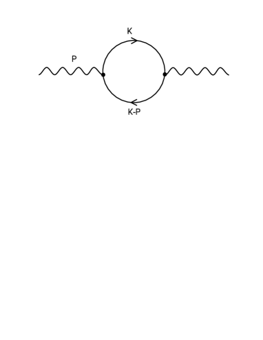
FIG. 1.: HTL photon self energy

Here we restrict ourselves to the longitudinal component of the self energy, i.e. $\Pi_{L}=\Pi_{00}$. Using the Keldysh representation and $S(K)=K\!\!\!\!/\,\>\Delta(K)$ for the fermion propagators, we find

$$\Pi_{R}^{L}(P)=-2ie^{2}\int\frac{d^{4}K}{(2\pi)^{4}}(q_{0}k_{0}+{\bf q}\cdot{\bf k})$$ (13)

$$\times\biggl{[}\Delta_{F}(K-P)\Delta_{R}(K)+\Delta_{A}(K-P)\Delta_{F}(K)\biggr{]}.$$ (14)

In the HTL approximation ($K\gg P$) the retarded ($\Pi_{R}=\Pi_{11}+\Pi_{12}$) and advanced ($\Pi_{A}=\Pi_{11}+\Pi_{21}$) self energies are given then by

$$\Pi_{R,A}^{L}(P)=-3m_{\gamma}^{2}\left(1-\frac{p_{0}}{2p}\ln\frac{p_{0}+p\pm i\epsilon}{p_{0}-p\pm i\epsilon}\right),$$ (15)

where the effective photon mass is given by an integral over the non-equilibrium Fermi distribution $f_{F}$

$$m_{\gamma}^{2}=\frac{4e^{2}}{3\pi^{2}}\int_{0}^{\infty}dk\,k\,f_{F}(k,x).$$ (16)

In equilibrium this expression reduces to $m_{\gamma}^{2}=e^{2}T^{2}/9$.

The symmetric self energy ($\Pi_{F}=\Pi_{11}+\Pi_{22}$) in the HTL limit can written as

$$\Pi_{F}^{L}(P)=2iA\,\frac{Im\,\Pi_{R}^{L}(P)}{p_{0}},$$ (17)

where the constant $A$ is given by

$$A=\frac{\int_{0}^{\infty}dk\,k^{2}\,f_{F}(k,x)\,[1-f_{F}(k,x)]}{\int_{0}^{\infty}dk\,k\,f_{F}(k,x)}.$$ (18)

In equilibrium this constant reduces to $A=2T$.

III Resummed photon propagator

The resummed photon propagator is constructed from the Schwinger-Dyson equation shown in Fig.2.

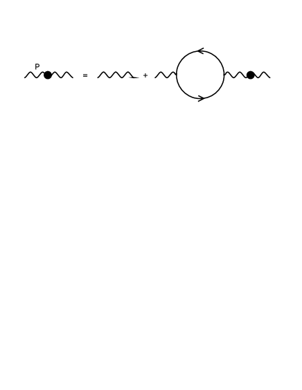
FIG. 2.: Resummed photon propagator

The Schwinger-Dyson equation for the resummed retarded and advanced propagators for longitudinal photons reads

$${D^{*}}_{R,A}^{L}=D_{R,A}^{L}+D_{R,A}^{L}\Pi_{R,A}^{L}{D^{*}}_{R,A}^{L}$$ (19)

leading to

$${D^{*}}_{R,A}^{L}(P)=\left[p^{2}+3m_{\gamma}^{2}\left(1-\frac{p_{0}}{2p}\ln\frac{p_{0}+p\pm i\epsilon}{p_{0}-p\pm i\epsilon}\right)\right]^{-1},$$ (20)

where the HTL photon self energy has been used. Apart from $m_{\gamma}$, defined by (16), this expression is identical to the equilibrium one.

The Schwinger-Dyson equation for the resummed symmetric propagator is given by

$${D^{*}}_{F}^{L}=D_{F}^{L}+D_{R}^{L}\Pi_{R}^{L}{D^{*}}_{F}^{L}+D_{F}^{L}\Pi_{A}^{L}{D^{*}}_{A}^{L}+D_{R}^{L}\Pi_{F}^{L}{D^{*}}_{A}^{L}.$$ (21)

This equation is solved by the following ansatz:

$${D^{*}}_{F}^{L}(P)=(1+2f_{B})\,\mbox{sgn}(p_{0})\,[{D^{*}}_{R}^{L}(P)-{D^{*}}_{A}^{L}(P)]$$ (22)

$$\;\;\;\;\;\;+\{\Pi_{F}^{L}(P)-(1+2f_{B})\,\mbox{sgn}(p_{0})\,[\Pi_{R}^{L}(P)-\Pi_{A}^{L}(P)]\}$$ (23)

$$\;\;\;\;\;\;\times{D^{*}}_{R}^{L}(P)\,{D^{*}}_{A}^{L}(P).$$ (24)

The product of a retarded and an advanced propagator at the same momentum $P$ may lead to a pinch singularity [7]. In equilibrium, however, the term in the curly brackets vanishes as a consequence of the Kubo-Martin-Schwinger boundary condition or the principle of detailed balance. Then the full symmetric propagator is given by the first line of (24), which is free of possible pinch problems and reflects the dissipation-fluctuation theorem [13].

The following relations can easily be shown to hold in general:

$${D^{*}}_{R}^{L}(P){D^{*}}_{A}^{L}(P)=\frac{{D^{*}}_{R}^{L}(P)-{D^{*}}_{A}^{L}(P)}{2i\,Im\,\Pi_{R}^{L}(P)},$$ (25)

$$\Pi_{R}^{L}(P)-\Pi_{A}^{L}(P)=2iIm\,\Pi_{R}^{L}(P).$$ (26)

Together with the expression (17) for the symmetric self energy we find from these relations that the symmetric non-equilibrium HTL resummed propagator can be written as

$${D^{*}}_{F}^{L}(P)=\frac{A}{p_{0}}\>[{D^{*}}_{R}^{L}(P)-{D^{*}}_{A}^{L}(P)].$$ (27)

Hence the symmetric propagator does not suffer from a pinch singularity even in non-equilibrium. This observation also holds for $p_{0}^{2}-p^{2}>0$, where $Im\,\Pi_{R}\sim\epsilon$ as following from (15), because of the cancellation of $Im\,\Pi_{R}$ according to (17), (24), and (26).

IV Electron interaction rate

As an example for the application of the non-equilibrium HTL resummation technique we consider the interaction or damping rate of an energetic electron in a non-equilibrium QED plasma. This quantity is one of the mostly studied within the HTL method. (For references see [3].) The HTL method does not lead to an infrared finite result in this case since there is not enough screening in the transverse part of the HTL photon propagator. After all we want to study this example, since we are only interested in the comparison between the equilibrium and the non-equilibrium case.

The interaction rate is defined by [14]

$$\Gamma(p)=-\frac{1}{2p}\,[1-f_{F}(p,x)]\>tr\,[P\!\!\!\!/\,\,Im\,\Sigma_{R}(p_{0}=p,{\bf p})],$$ (28)

where $\Sigma_{R}$ is the retarded electron self energy. Using only bare propagators the lowest order contribution to $Im\,\Sigma_{R}$ comes from the two-loop diagram of Fig.3.

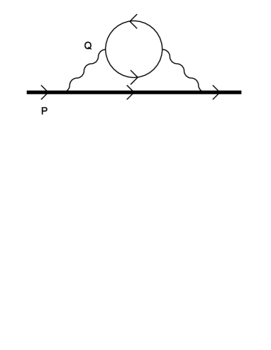
FIG. 3.: Lowest order contribution of the electron self energy to the electron interaction rate within naive perturbation theory

This diagram contains a dangerous pinch term coming from the product of a retarded and an advanced bare propagator at the same momentum $Q$ [15]:

$$D^{L}_{R}(Q)D^{L}_{A}(Q) = \frac{1}{Q^{2}+i{\rm sgn}(q_{0})\epsilon}\,\,\frac{1}{Q^{2}-i{\rm sgn}(q_{0})\epsilon}$$ (29)

$$\rightarrow [\delta(Q^{2})]^{2}.$$ (30)

In equilibrium this term vanishes due to detailed balance.

Applying the HTL method to the electron interaction rate results in using the one-loop diagram of Fig.4 containing a resummed photon propagator for the electron self energy [3, 14]. Owing to the non-zero imaginary part of the HTL photon self energy appearing in the resummed photon propagator this diagram exhibits an imaginary part. Since there is no pinch singularity in the HTL resummed photon propagator this diagram is also free of pinch singularities. In other words, the use of the HTL method to lowest order reduces two-loop diagrams, containing possible pinch singularities, to one-loop diagrams with resummed propagators, where pinch terms are absent.

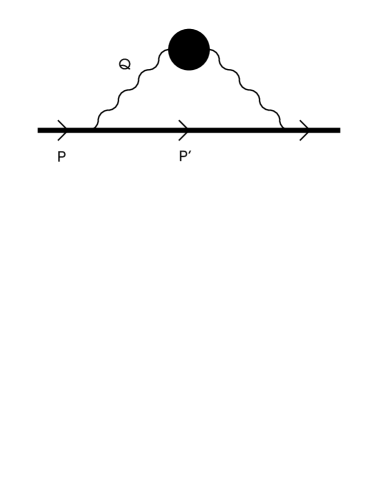
FIG. 4.: Lowest order contribution of the electron self energy to the electron interaction rate within the HTL method

Following the equilibrium calculation [3, 14], we end up with the following result for the non-equilibrium interaction rate of an energetic electron:

$$\Gamma_{neq}(p)\simeq\frac{e^{2}A}{4\pi}\>\ln\frac{const}{e}.$$ (31)

The logarithm in this expression reflects the presence of an infrared singularity, which has been regularized by assuming an infrared cutoff of the order $e^{2}T$. The constant under the logarithm cannot be calculated within the HTL method. As expected this result reduces to the equilibrium one [3], if we replace $A$ by $2T$..

Pinch terms may arise, however, in higher order contributions of the HTL perturbation theory, such as the one shown in Fig.5, where the product of a retarded HTL and an advanced HTL propagator at the same momentum $Q$ shows up.

Resumming the photon self energy $\bar{\Pi}$, which contains HTL electron propagators and HTL vertices, leads to a dressed propagator beyond the HTL resummation. The symmetric component of this propagator reads

$${D^{**}}_{F}^{L}(Q)=\frac{A}{q_{0}}\,[{D^{**}}_{R}^{L}(Q)-{D^{**}}_{A}^{L}(Q)]$$ (32)

$$+\{\bar{\Pi}_{F}^{L}(Q)-\frac{A}{q_{0}}\,[\bar{\Pi}_{R}^{L}(Q)-\bar{\Pi}_{A}^{L}(Q)]\}\,{D^{**}}_{R}^{L}(Q)\,{D^{**}}_{A}^{L}(Q).$$ (33)

If $\bar{\Pi}_{F}$ is proportional to $Im\,\bar{\Pi}_{R}$ as in (17), this propagator would not contain a pinch term.

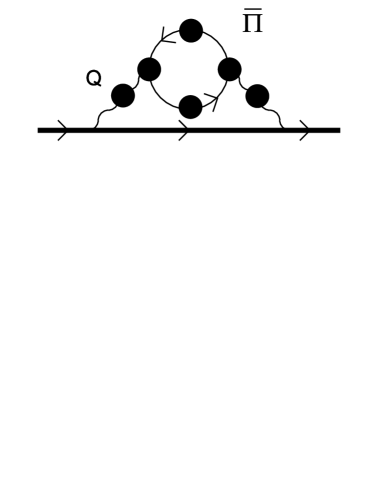
FIG. 5.: Photon self energy $\bar{\Pi}$

V Ward identities

Finally we will show that the HTL electron self energy and the HTL electron-photon vertex fulfill the same Ward identities in non-equilibrium as in equilibrium. For this purpose we write the one-particle-irreducible vertex functions as [13, 16]

$$\Gamma_{R} = \frac{1}{2}(\Gamma_{111}+\Gamma_{112}+\Gamma_{211}+\Gamma_{212}$$ (35)

$$\;\;\;\;-\Gamma_{121}-\Gamma_{122}-\Gamma_{221}-\Gamma_{222}),$$

$$\Gamma_{Ri} = \frac{1}{2}(\Gamma_{111}+\Gamma_{112}+\Gamma_{121}+\Gamma_{122}$$ (37)

$$\;\;\;\;-\Gamma_{211}-\Gamma_{212}-\Gamma_{221}-\Gamma_{222}),$$

$$\Gamma_{Ro} = \frac{1}{2}(\Gamma_{111}+\Gamma_{121}+\Gamma_{211}+\Gamma_{221}$$ (39)

$$\;\;\;\;-\Gamma_{112}-\Gamma_{122}-\Gamma_{212}-\Gamma_{222}).$$

Here only the three retarded combinations of the seven independent components of the vertex in the Keldysh representation are shown. Using the HTL approximation for the vertices and the electron self energy, we can show the following Ward identities (without performing the loop integrations explicitly)[17]:

$$K_{\phi}\Gamma^{\phi}_{R}(-Q,P,K) = -ie(\Sigma_{A}(P)-\Sigma_{R}(Q)),$$ (40)

$$K_{\phi}\Gamma^{\phi}_{Ri}(-Q,P,K) = -ie(\Sigma_{A}(P)-\Sigma_{A}(Q)),$$ (41)

$$K_{\phi}\Gamma^{\phi}_{Ro}(-Q,P,K) = -ie(\Sigma_{R}(P)-\Sigma_{R}(Q)),$$ (42)

which hold in equilibrium as well as non-equilibrium.

VI Conclusions

In the present work we have extended the HTL resummation technique to non-equilibrium situations assuming quasistatic distribution functions. We are not able to treat the evolution of the system towards equilibrium, but can describe properties of a relativistic non-equilibrium plasma, where the equilibration is slow compared to the process under investigation. Such a situation might be realized for example in a chemically non-equilibrated QPG produced in the fireball of a relativistic heavy ion collision.

Starting from the RTF we have demonstrated the usefulness of the Keldysh representation for the HTL method in equilibrium as well as non-equilibrium.

The non-equilibrium HTL resummation technique differs from the equilibrium one only by two aspects:

1. There are new effective masses defined by integrals over the non-equilibrium distributions appearing in the HTL self energies.

2. There is a constant factor $A$, also defined by integrals over the distributions, in the symmetric self energy and the resummed symmetric propagator, which reduces to $2T$ in equilibrium.

We have shown that there are no pinch terms in the HTL resummed propagators. Therefore pinch singularities are absent in quantities calculated from one-loop HTL self energies, such as the electron interaction rate. A similar result was found in the case of the photon production rate [6] and the collisional energy loss of energetic quarks [18].

Beyond leading order in the HTL perturbation theory we expect also the absence of pinch terms using a higher order resummation scheme.

Finally we have given the Ward identities for the HTL electron self energy and the HTL electron-photon vertex, which hold in equilibrium as well as non-equilibrium.

REFERENCES

- [1]
- [2] E. Braaten and R.D. Pisarski, Nucl. Phys. B337, 569 (1990).
- [3] M.H. Thoma, in Quark-Gluon Plasma 2, edited by R. Hwa (World Scientific, Singapore 1995), p.51.
- [4] K. Geiger, Phys. Rep. 258, 238 (1995); X.N. Wang, Phys. Rep. 280, 287 (1997).
- [5] M.E. Carrington, H. Defu, and M.H. Thoma, hep-ph/9708363, Eur. Phys. J. C (in press).
- [6] R. Baier, M. Dirks, K. Redlich, and D. Schiff, Phys. Rev. D 56 (1997) 2548.
- [7] N.P. Landsmann and C.G. van Weert, Phys. Rep. 145, 141 (1987).
- [8] M. Le Bellac and H. Mabilat, Z. Phys. C 75, 137 (1997).
- [9] K. Chou, Z. Su, B. Hao, and L. Yu, Phys. Rep. 118, 1 (1985).
- [10] C. Greiner and S. Leupold, hep-ph/9804239.
- [11] T.S. Biró, E. van Doorn, B. Müller, M.H. Thoma, and X.N. Wang, Phys. Rev. C 48, 1275 (1993).
- [12] T.S. Biró, B. Müller, and X.N. Wang, Phys. Lett. B283, 171 (1992).
- [13] M.E. Carrington and U. Heinz, Eur. Phys. J. C 1, 619 (1998).
- [14] E. Braaten and M.H. Thoma, Phys. Rev. D 44, 1298 (1991).
- [15] T. Altherr and D. Seibert, Phys. Lett. B 333, 149 (1994).
- [16] H. Defu and U. Heinz, Eur. Phys. J. C 4, 129 (1998). (in press).
- [17] M.E. Carrington, H. Defu, and M.H. Thoma, hep-ph/9801103, Phys. Rev. D (in press).
- [18] R. Baier, M. Dirks, and K. Redlich, in preparation.