Abstract

We investigate the occurrence of power terms in the running QCD coupling $\alpha_{s}(p)$ by analysing non-perturbative measurements at low momenta ($p\gtrsim 2{\rm GeV}$) obtained from the lattice three-gluon vertex. Our exploratory study provides some evidence for power contributions to $\alpha_{s}(p)$ proportional to $1/p^{2}$. Possible implications for physical observables are discussed.

1 Introduction

The standard procedure to parametrise non-perturbative QCD effects in terms of power corrections to perturbative results is based on the Operator Product Expansion (OPE). In this framework, the powers involved in the expansion are expected to be uniquely fixed by the symmetries and the dimension of the relevant operator product. It should be noted that, due to the asymptotic nature of QCD perturbative expansions, power corrections are reshuffled between operators and coefficient functions in the OPE [1].

The above picture has recently been challenged [2, 3, 4]. It was pointed out that power corrections which are not a priori expected from the OPE may in fact appear in the expansion of physical observables. Such terms may arise from (UV-subleading) power corrections to $\alpha_{s}(p)$, corresponding to non-analytical contributions to the $\beta$-function. To illustrate this point, consider for example a typical contribution to a condensate of dimension $2\sigma$:

$$\int_{\rho\Lambda^{2}}^{Q^{2}}\frac{dp^{2}}{p^{2}}(\frac{p^{2}}{Q^{2}})^{\sigma}\alpha_{s}(\frac{p^{2}}{\Lambda^{2}})\;.$$ (1)

A power contribution to $\alpha_{s}(\frac{p^{2}}{\Lambda^{2}})$ of the form $(\frac{\Lambda^{2}}{p^{2}})^{z}$ would generate (from the UV limit of integration) a contribution to the condensate proportional to $(\frac{\Lambda^{2}}{Q^{2}})^{z}$. The fact that the dimension of such a term would be independent of $\sigma$ indicates that this contribution would be missed in a standard OPE analysis.

Note that in the above manipulations $z$ could be in principle any (real) number. The value $z=1$ may in fact play a special role (see the discussion in Section 2), as it would result in $\frac{\Lambda^{2}}{p^{2}}$ contributions to physical processes whose existence has been conjectured for a long time, mainly in the framework of the UV renormalon [5].

Clearly, the existence of $\sigma$-independent power corrections, if demonstrated, would have a major impact on our understanding of non-perturbative QCD effects and may affect QCD predictions for several processes. For example, $\frac{\Lambda^{2}}{Q^{2}}$ contributions may be relevant for the analysis of $\tau$ decays [6, 2].

Although the size of such corrections could in principle be estimated directly from experimental data, it would be highly desirable to develop a theoretical framework where the occurrence of these effects is demonstrated and estimates are obtained from first principles QCD calculations. Some steps in this direction were performed in [7, 4], where some evidence for an unexpected $\frac{\Lambda^{2}}{Q^{2}}$ contribution to the gluon condensate was obtained through lattice calculations.

The aim of the present work is to test a method to detect the presence of power corrections in the running QCD coupling. Non-perturbative lattice estimates of the coupling at low momenta are compared with perturbative formulae. Although at this stage our work is exploratory in nature and further simulations will be required to obtain a conclusive answer, our analysis provides some preliminary evidence for power corrections. The final goal is to investigate the possible link between OPE-independent power corrections to physical observables and power terms in the running coupling.

The paper is organised as follows: in Section 2 we briefly review some theoretical arguments in support of power corrections to $\alpha_{s}(p)$, illustrating the special role that may be played by $\frac{\Lambda^{2}}{p^{2}}$ terms. In Section 3 we explain the meaning of the lattice data and our strategy for the analysis. Some preliminary evidence for power corrections is discussed. Finally, in Section 4 we draw our conclusions. The appendix contains some technical details.

2 Clues for $\frac{\Lambda^{2}}{p^{2}}$ Corrections to $\alpha_{s}(p)$

Power corrections to $\alpha_{s}(p)$ can be shown to arise naturally in many physical schemes [8, 9]. The occurrence of such corrections cannot be excluded a priori in any renormalisation scheme. Clearly, given the non-analytic dependence of $(\frac{\Lambda^{2}}{p^{2}})^{z}$ terms on $\alpha_{s}$, power corrections cannot be generated or analysed in perturbation theory. In particular, the non-perturbative nature of such effects makes it very hard to assess their dependence on the renormalisation scheme, which is only very weakly constrained by the general properties of the theory.

As discussed in the following, despite the arbitrariness a priori of the exponent $z$, several arguments have been put forward in the past to suggest that a likely candidate for a power correction to $\alpha_{s}(p)$ would be a term of order ${\Lambda^{2}}/{p^{2}}$, i.e. $z=1$.

2.1 Static Quark Potential and Confinement

Consider the interaction of two heavy quarks in the static limit (for a more detailed discussion see [10]). In the one-gluon-exchange approximation, the static potential $V(r)$ can be written as

$$V(r)\,\propto\,\alpha_{s}\ \int d^{3}k\,\frac{\exp^{i\vec{k}\cdot\vec{r}}}{|\vec{k}|^{2}}.$$ (2)

Clearly the above formula yields the Coulomb potential $V(r)\approx 1/r$. Using standard arguments of renormalon analysis, one may consider a generalisation of (2) obtained by replacing $\alpha_{s}$ with a running coupling:

$$V(r)\,\propto\,\int d^{3}k\,\alpha_{s}(|\vec{k}|^{2})\,\frac{\exp^{i\vec{k}\cdot\vec{r}}}{|\vec{k}|^{2}}.$$ (3)

The presence of a power correction term of the form $\alpha_{s}(k^{2})\propto{\Lambda^{2}}/{k^{2}}$ would generate a linear confining potential $V(r)\sim Kr$. Note that a standard renormalon analysis of (3) (see [10] for the details) reveals contributions to the potential containing various powers of $r$, but a linear contribution is missing. This is a typical result of renormalon analysis: renormalons can miss important pieces of non-perturbative information.

2.2 An Estimate from the Lattice

The lattice community has been made aware for some time of the possibility of non-perturbative contributions to the running coupling; for a clear discussion see [11]. Consider the “force” definition of the running coupling:

$$\alpha_{q\bar{q}}(Q)=\frac{3}{4}r^{2}\frac{dV(r)}{dr}\;\;\;\;\;(Q=\frac{1}{r}),$$ (4)

where again $V(r)$ represents the static interquark potential. By keeping into account the string tension contribution to $V(r)$, which can be measured in lattice simulations, one obtains a $1/Q^{2}$ contribution, whose order of magnitude is given by the string tension itself. Ironically, this term has been mainly considered as a sort of ambiguity, resulting in an indetermination in the value of $\alpha(Q)$ at a given scale. From a different point of view, such a term could be interpreted as a clue for the existence of a $\frac{\Lambda^{2}}{p^{2}}$ contribution, and it also provides an estimate for the expected order of magnitude of it, at least in one (physically sound) scheme.

2.3 Landau pole and analyticity.

It is well known that perturbative QCD formulae for the running of $\alpha_{s}$ inevitably contain singularities, which are often referred to as the Landau pole. The details of the analytical structure depend on the order at which the $\beta$-function is truncated and on the particular solution chosen. The existence of an interplay between the analytical structure of the perturbative solution and the structure of non-perturbative effects has been advocated for a long time [12]. To illustrate this idea, consider the one-loop formula for the running coupling $\alpha_{s}(p)$:

$$\alpha_{s}(p^{2})~{}=~{}{1\over b_{0}\ \log(\frac{p^{2}}{\Lambda^{2}})}.$$ (5)

Here the singularity is a simple pole, which can be removed if one redefines $\alpha_{s}(p)$ according to the following prescription:

$$\alpha_{s}(p^{2})~{}=~{}{1\over b_{0}\ \log(\frac{p^{2}}{\Lambda^{2}})}+{\Lambda^{2}\over b_{0}(\Lambda^{2}-p^{2})},$$ (6)

where a power correction of the asymptotic form $\frac{\Lambda^{2}}{p^{2}}$ appears. However, the sign of such a correction is the opposite of what one would expect from the results of [4] and from the considerations in Section 2.1, so that in the end one could envisage a more general formula for the regularised coupling:

$$\alpha_{s}(p^{2})~{}=~{}{1\over b_{0}\ \log(\frac{p^{2}}{\Lambda^{2}})}+{\Lambda^{2}\over b_{0}(\Lambda^{2}-p^{2})}+c\ {\Lambda^{2}\over p^{2}}.$$ (7)

The message from (7) is that the perturbative coupling is not defined at the $\frac{\Lambda^{2}}{p^{2}}$ level, so the coefficient of the power correction is unconstrained, even after imposing the cancellation of the pole.

At higher perturbative orders one encounters multiple singularities, which include an unphysical cut. There are several ways to regularise them. In particular, the method discussed in [12] combines a spectral-representation approach with the Renormalization Group. The method was originally formulated for QED, but it has recently been extended to the QCD case [13].

Other approaches can be conceived to achieve a systematic regularisation of the singularities arising from the Landau pole, order by order in perturbation theory. In this way one obtains formulae for $\alpha_{s}(p)$ that are well-defined at all momentum scales.

Such formulae would be quite useful in the framework of our study, since power corrections are expected to be sizeable at scales close to the location of the Landau pole. However, for the purpose of the preliminary investigation discussed in the present paper, we shall limit ourselves to a simpler approach, where one tries to fit the data by simply adding power corrections to the perturbative expressions, without attempting a regularisation of the Landau pole.

3 Lattice Data and Power Corrections

3.1 $\alpha_{s}$ on the Lattice

Several methods for computing $\alpha_{s}(p)$ non-perturbatively on the lattice have been proposed in recent years [14, 15, 16, 17, 18]. In most cases, the goal of such studies is to obtain an accurate prediction for $\alpha_{s}(M_{Z})$, i.e. the running coupling at the $Z$ peak, which is a fundamental parameter in the standard model. For this reason, lattice parameters are usually tuned as to allow the computation of $\alpha_{s}(p)$ at momentum scales of at least a few GeVs, where the two-loop asymptotic behaviour is expected to dominate and power contributions are suppressed. However, the same methods can in principle be applied to the study of $\alpha_{s}(p)$ at lower momentum scales, where power-like terms may be sizeable. For this purpose, the best method is one where one can measure $\alpha_{s}(p)$ in a wide range of momenta from a single Monte Carlo data set.

One method which fulfills the above criterion is the determination of the coupling from the renormalised lattice three-gluon vertex function [18, 19]. This is achieved by evaluating two- and three-point off-shell Green’s functions of the gluon field in the Landau gauge, and imposing non-perturbative renormalisation conditions on them, for different values of the external momenta. By varying the renormalisation scale $p$, one can determine $\alpha_{s}(p)$ for different momenta from a single simulation. Obviously the renormalisation scale must be chosen in a range of lattice momenta such that both finite volume effects and discretisation errors are under control. Such a definition of the coupling corresponds to a momentum-subtraction renormalisation scheme in continuum QCD [20]. It should be noted that in this scheme the coupling is a gauge-dependent quantity. One consequence of this fact is that $1/p^{2}$ corrections should be expected, based on OPE considerations. We will return to this issue when drawing our conclusions.

The numerical results for $\alpha_{s}(p)$ that we use for our investigation were obtained from 150 configurations on a $16^{4}$ lattice at $\beta=6.0$.

For full details of the method we refer the reader to Ref. [19], where such results were first presented. In order to detect violations of rotational invariance, different combinations of lattice vectors have sometimes been used for a fixed value of $p^{2}$. This accounts for the graphical “splitting” of some data points.

3.2 Models for Power Corrections

As mentioned at the end of Section 2.3, in the present work we shall not address the general problem of defining a regular coupling at all scales. For the purpose of our preliminary investigation, we shall compare the non-perturbative data for $\alpha_{s}$ with simple models obtained by adding a power correction term to the perturbative formula at a given order. In order to identify momentum intervals where our ansatz fits the data, one should keep in mind that the momentum range should start well above the location of the perturbative Landau pole, but it should nonetheless include low scales where power corrections may still be sizeable. The requirement of keeping the effects of the finite lattice spacing under control in the numerical data for $\alpha_{s}$ induces a natural UV cutoff on the momentum range. It is reassuring that intervals that fulfill these requirements can be identified, as specified in the following.

One problem in this approach is the possible interplay between a description in terms of (non-perturbative) power corrections and our ignorance about higher orders of perturbation theory. In particular, for the scheme that we consider, the three-loop coefficient of the $\beta$-function is not known. Knowledge of such a coefficient would allow to perform a more reliable comparison of our estimates for the $\Lambda$ parameter in our scheme with lattice determinations of $\Lambda$ in a different scheme, for which the three-loop result is available [21]. In fact, although matching the $\Lambda$ parameter between different schemes only requires a one-loop computation (because of asymptotic freedom), the reliability of such a comparison rests on the assumption that the value of $\Lambda$ in each scheme is fairly stable with respect to the inclusion of higher orders, which in turn implies that a sufficient number of perturbative orders has been considered in the definition of $\Lambda$. In practice, when working at two- or three-loop order, the value of $\Lambda$ is still quite sensitive to the order of the calculation. For this reason, in the formulae for $\alpha_{s}(p)$ we shall append a subscript to the parameter $\Lambda$, to remind the reader that the value of such a parameter is expected to carry a sizeable dependence on the order of the perturbative calculation.

Even within such limitations, in the following we will argue that it is possible to estimate the impact of three-loop effects in our model and that a description with power corrections seems to be stable with respect to the inclusion of such effects.

3.3 Two-loop Analysis

At the two-loop level, we consider the following formula:

$$\alpha_{s}(p)\,=\,\frac{1}{b_{0}\,\log(p^{2}/\Lambda_{2l}^{2})}\,-\,\frac{b_{1}}{b_{0}}\frac{\log(\log(p^{2}/\Lambda_{2l}^{2}))}{(b_{0}\,\log(p^{2}/\Lambda_{2l}^{2}))^{2}}\,+\,c_{2l}\,\frac{\Lambda_{2l}^{2}}{p^{2}}$$ (8)

By fitting our data to (8) we obtain two sets of estimates for the parameters ($\Lambda_{2l}$,$c_{2l}$), namely ($0.84(1)$,$0.31(3)$) and ($0.73(1)$,$0.99(7)$). The two results correspond to comparable values for $\chi^{2}_{dof}$, and in both cases we obtain $\chi^{2}_{dof}\leq 1.8$. In both cases, the momentum window extends up to $p\sim 3$ GeV. We take the first set of values as our best estimate of the parameters as the corresponding value of $\Lambda_{2l}$ is close to what is obtained from a “pure” two-loop fit, i.e. $\Lambda_{2l}$ is stable with respect to the introduction of power corrections. Our choice for the value of $\Lambda_{2l}$ will be a posteriori supported also by independent considerations at the three-loop level. The momentum range that we are able to describe ($1.8-3.0\ {\rm GeV}$) is fully consistent with what one would expect from general considerations based on the value of the UV lattice cut-off and the value of $\Lambda_{2l}$. Notice that choosing between the two sets of values makes quite a difference in the UV region, where power effects are largely suppressed.

In summary, a two-loop description with power corrections based on (8) fits well the data in a consistent momentum range. Our best fit of the data to (8) is shown in Figure 1. We were also able to check that if one tries to determine the exponent $z$ of the power correction $(\frac{\Lambda_{2l}^{2}}{p^{2}})^{z}$ from the fit, the best description of the data is obtained for $z\approx 1$. We interpret this result as a confirmation of our theoretical prejudice $z=1$. However, one should note that since that the quality of our data makes a full three-parameter fit very hard, the above check of the value of $z$ and any other three-parameter fit that we mention in the following sections were in fact obtained by performing a very large number of two-parameter fits, corresponding to different (fixed) values of the third parameter.

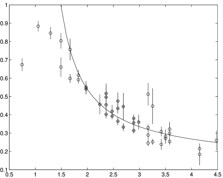
Figure 1: The best fit to (8). The crossed-circled points indicate the fitting range.

3.4 Three-loop Analysis

As already mentioned, a major obstacle for a three-loop analysisis is the fact that the first non-universal coefficient $b_{2}$ of the perturbative $\beta$-function is not known for our scheme.

In order to gain insight, we start by performing a two-parameter fit to the standard three-loop expression for $\alpha_{s}(p)$, where the fitting parameters are $\Lambda_{3l}$ and the unknown coefficient $b_{2}$. We call $b_{2}^{eff}$ the fit estimate for $b_{2}$, to emphasise that we expect the effective value $b_{2}^{eff}$ to provide an order of magnitude estimate of the true (unknown) coefficient $b_{2}$. Our best estimate for $\Lambda_{3l}$ and $b_{2}$ is $\Lambda_{3l}=0.72(1)$, $b_{2}^{eff}=1.3(1)$, with $\chi^{2}_{dof}\approx 1.8$ (see the dashed curve in Fig. 2). The error quoted for the fit parameters should always be interpreted within the effective description provided by the relevant formula.

The momentum range where we obtain the best description of the data is $p\sim 2-3$ GeV. Our result for $\Lambda_{3l}$ provides (via perturbative matching) an estimate for $\Lambda_{\overline{MS}}$, in very good agreement with the estimate in [21], which was obtained from the computation of the $\Lambda$ parameter in a completely different scheme. Although both estimates are affected by our ignorance of higher loop effects, and our estimate also depends on the extra parameter $b_{2}^{eff}$, the agreement between the two results appears remarkable. In order to investigate the reliability of $b_{2}^{eff}$ as an estimate of $b_{2}$, we discuss in the appendix an argument which appears to provide a lower bound for the value of $b_{2}$ in our scheme, namely $b_{2}\gtrsim 0.3$. Our value for $b_{2}^{eff}$ is therefore consistent with such a bound.

Having obtained comparable values for $\chi^{2}_{dof}$ from the two-loop analysis with power corrections and from the “pure” three-loop analysis, one may be led to consider our results as evidence against the existence of power corrections, since so far they simply appear to provide an effective description of three-loop effects.

However, we will argue now that there is room for power corrections even at the three-loop level. To this aim, consider the following three-loop formula with a power correction:

$$\alpha_{s}(p) = \frac{1}{b_{0}\,L}\,-\,\frac{b_{1}}{b_{0}}\frac{\log(L)}{(b_{0}\,L)^{2}}$$ (9)

$$+\,\frac{1}{(b_{0}\,L)^{3}}\,\left(\frac{b_{2}^{eff}}{b_{0}}+\frac{b_{1}^{2}}{b_{0}^{2}}(\log^{2}(L)-\log(L)+1)\right)$$

$$+\,c_{3l}\,\frac{\Lambda_{3l}^{2}}{p^{2}},$$

where $L=\log(p^{2}/\Lambda_{3l}^{2})$ and $b_{2}^{eff}$ is again to be determined from a fit.

Fitting the data to (9), we obtain $\Lambda_{3l}=0.72(1)$, $b_{2}^{eff}=1.0(1)$ and $c_{3}=0.41(2)$, with $\chi^{2}_{dof}\approx 1.8$, in a momentum range $1.8-3.0\,{\rm GeV}$ (see Fig. 2). The above result was in practice obtained by performing a large number of two-parameter fits for $b_{2}^{eff}$ and $c_{3}$, for fixed values of $\Lambda_{3l}$. The range of trial values for $\Lambda_{3l}$ was suggested by the results of the “pure” three-loop fit.

We note the following:

1. the value for the scale parameter $\Lambda_{3l}$ is fully consistent with the previous determination from the “pure” three-loop description;

2. the value for $b_{2}^{eff}$ is also reasonably stable with respect to the previous determination and it is also consistent with the approximate lower bound for $b_{2}$ discussed in the appendix;

3. by comparing results from fits to (8) and (9), it emerges that

   $$c_{2}\Lambda_{2l}^{2}=0.22(2)\,{\rm GeV}^{2}\sim c_{3}\Lambda_{3l}^{2}=0.21(2)\,{\rm GeV}^{2}.$$ (10)

   This approximate equality gives us confidence in the presence of power corrections, as it indicates that the power terms providing the best fit to (8) and (9) are numerically equal. In other words, there appears to be no interplay between the indetermination connected to the perturbative terms and the power correction term, within the precision of our data, thus suggesting that a genuine $\frac{\Lambda^{2}}{p^{2}}$ correction is present in the data.

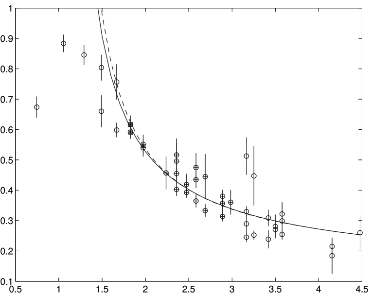
Figure 2: Fits to (9) (solid line) versus a pure three-loop fit (dashed line). The crossed-circled points are consistent with both ansatze, while the star-circled one is best fitted by (9).

Finally, the coefficient of the power correction is of the order of magnitude expected from the arguments in sections 2.1 and 2.2, that is, it is comparable to the standard estimate for the string tension squared.

One may argue at this point that at the two-loop level we had to choose between two sets of values for ($\Lambda_{2l}$,$c_{2l}$), and that our choice is crucial for the validity of (10). An a posteriori justification for our choice can be obtained from the following test: we plot a few values for $\alpha_{s}(p)$ as generated by the “pure” three-loop formula for $\Lambda_{3l}=0.72$ and $b_{2}=1.0$. Then, by fitting such points to the “pure” two-loop formula, one gets $\Lambda_{2l}\approx 0.84$, i.e. the value for which (10) holds.

4 Conclusions

We have discussed an exploratory investigation of power corrections in the running QCD coupling $\alpha_{s}(p)$ by comparing non-perturbative lattice results with theoretical models. Some evidence was found for $1/p^{2}$ corrections, whose size was consistent with what is suggested by simple arguments from the static potential.

At the technical level, our results need further confirmation from the analysis of a larger data set and a study of the dependence of the fit parameters on the ultraviolet and infrared lattice cutoff. Assuming our findings are confirmed at the technical level, one needs to address the issue of assessing the scheme dependendence of our results. As already discussed, the non-perturbative nature of power corrections makes it very hard to formulate any theoretical procedure to estimate the impact of scheme dependence. The best one can do at this stage is to consider different renormalisation schemes and definitions of the coupling and gather numerical evidence and formal arguments supporting power corrections to $\alpha_{s}(p)$. In this way, scheme-independent features may eventually be identified. For example, on the basis of our results, we note the following:

• Theoretical arguments suggest $1/p^{2}$ corrections both for the coupling as defined from the static potential and for the one obtained from the three-gluon vertex. The arguments for the former case were outlined in Sections 2.1 and 2.2. As far as the coupling from the three-gluon vertex is concerned, $1/p^{2}$ corrections appear in an OPE analysis if one keeps into account the fact that such a coupling is a priori gauge dependent, so that a dimension 2 condensate appears in the relevant OPE.

• In the static potential case, the theoretical argument also provides an estimate for the order of magnitude of the coefficient of the $1/p^{2}$ correction, while in the three-gluon vertex case the OPE argument provides no estimate for it, suggesting instead that it may depend on the gauge. However, our numerical result in the Landau gauge is in striking agreement with the estimate for the static potential case. Although such an agreement may of course be accidental, it calls for further investigation, which may be performed by attempting a similar calculation in a different gauge.

The issue of scheme dependence will be the focus of our future work.

5 Acknowledgements

We thank B. Alles, H. Panagopoulos and D. G. Richards for allowing us to use data files containing the results of Ref. [19]. C. Parrinello acknowledges the support of PPARC through an Advanced Fellowship. C. Pittori thanks J. Cugnon and the “Institut de Physique de l’Université de Liège au Sart Tilman” and acknowledges the partial support of IISN. We thank C. Michael for stimulating discussions.

Appendix A

Consider the perturbative matching between our scheme and the $\overline{MS}$ scheme

$$\alpha_{{}^{\widetilde{MOM}}}\,=\,\alpha_{{}^{\overline{MS}}}\,+\,c_{1}\,\alpha_{{}^{\overline{MS}}}^{2}\,+\,c_{2}(b_{2})\,\alpha_{{}^{\overline{MS}}}^{3}\,+\,O(\alpha_{s}^{4})$$

As it is well known, $c_{1}$ determines the ratio of the $\Lambda$ parameters in the different schemes, while $c_{2}$ depends on $c_{1}$ and the difference between the value of $b_{2}$ in our scheme and $b_{2}^{\overline{MS}}$. We assume that at very high momentum values ($p>150$ GeV) the running coupling follows the three-loop asymptotic formula. Then if one takes the value for $\Lambda_{\overline{MS}}$ from [21] and the value for $\Lambda_{\widetilde{MOM}}$ in our scheme from the perturbative matching, the only unknown parameter in the above expression is the value of $b_{2}$ in our scheme. By demanding that at the two-loop level the expansion of one coupling in powers of the other is still convergent (i.e. the convergence is better at two loops than at one loop as the series are not yet displaying their asymptotic nature) we obtain an approximate lower bound for the unknown coefficient as $b_{2}\gtrsim 0.3$. We have checked that such a technique provides sensible results for every couple of couplings for which a two-loop matching is known.

References

-
[1]
For reviews and classic references see:
V.I. Zakharov, Nucl. Phys. B385 (1992) 452;
A.H. Mueller, in QCD 20 years later, vol. 1 (World Scientific, Singapore 1993). B. Lautrup, Phys. Lett. 69B (1977) 109; G. Parisi, Phys. Lett. 76B (1977) 65; Nucl. Phys. B150 (1979) 163; G. t’Hooft, in The Whys of Subnuclear Physics, Erice 1977, ed A. Zichichi, (Plenum, New York 1977); M. Beneke and V.I. Zakharov, Phys. Lett. 312B (1993) 340; M. Beneke Nucl. Phys. B307 (1993) 154; A. H. Mueller, Nucl. Phys. B250 (1985) 327; Phys. Lett. 308B (1993) 355; G. Grunberg, Phys. Lett. 304B (1993) 183; Phys. Lett. 325B (1994) 441. - [2] R. Akhoury and V.I. Zakharov, hep-ph/9705318.
- [3] G.Grunberg, hep-ph/9705290; hep-ph/9705460.
- [4] G Burgio, F. Di Renzo, G. Marchesini and E. Onofri, Phys. Lett. 422B (1998) 219.
- [5] A. H. Mueller, in QCD 20 years later, vol. 1 and references therein. R. Akhoury and V.I. Zakharov, hep-ph/9710257.
- [6] G. Altarelli, P. Nason, G. Ridolfi, Zeit. Phys. C68 (1995) 257.
- [7] An early evidence of such a contribution was reported in G.P. Lepage and P. Mackenzie, Nucl. Phys. Proc. Suppl. 20 (1991) 173, although the perturbative series was not managed up to high orders.
- [8] Yu.L. Dokshitzer, G. Marchesini and B.R. Webber, Nucl. Phys. B469 (1996) 93
- [9] S.J. Brodsky, G.P. Lepage and P.B. Mackenzie, Phys. Rev. D 28 (1983) 228.
- [10] R. Akhoury and V.I. Zakharov, hep-ph/9710487.
- [11] C. Michael, Nucl. Phys. Proc. Suppl. 42 (1995) 147.
- [12] P. Redmond, Phys. Rev. D 112 (1958) 1404; N.N. Bogoliubov, A.A. Logunov and D.V. Shirkov, Sov. Phys. JETP 37 (1959) 805.
- [13] D.V. Shirkov and I.L. Solovtsov, Phys. Rev. Lett. 79 (1997) 1209
- [14] A.X. El-Khadra et al., Phys. Rev. Lett. 69 (1992) 729.
- [15] M. Lüscher et al., Nucl. Phys. B413 (1994) 481.
- [16] G.S. Bali and K. Schilling, Phys. Rev. D47 (1993) 661.
- [17] S.P. Booth et al., Phys. Lett. B294 (1992) 385.
- [18] C. Parrinello, Phys. Rev. D50 (1994) 4247.
- [19] B. Allés, D. S. Henty, H. Panagopoulos, C. Parrinello, C. Pittori, D. G. Richards, Nucl. Phys. B502 (1997) 325
- [20] R. Dashen and D.J. Gross, Phys. Rev. D23 (1981) 2340
- [21] S. Capitani, M. Guagnelli, M. Luescher, S. Sint, R. Sommer, P. Weisz and H. Wittig, Nucl. Phys. Proc. Suppl. 63 (1998) 153.