August 1998

DESY-98-102

TAUP 2515/98

hep-ph/9808257

THE EFFECT OF SCREENING
ON THE $\mathbf{x}$ AND $\mathbf{Q}^{2}$ BEHAVIOUR
OF $\mathbf{F_{2}}$ SLOPES

E.  G O T S M A N^a) 1),        E.  L E V I N${}^{a)\,b)\,2)}$,

U.  M A O R^a) 3)    and    E.  N A F T A L I^a) 4)

a)    School of Physics and Astronomy
Raymond and Beverly Sackler Faculty of Exact Science
Tel Aviv University, Tel Aviv, 69978, ISRAEL
b)    DESY Theory Group
22603, Hamburg, GERMANY

Abstract: A systematic study of $\frac{\partial F_{2}(x,Q^{2})}{\partial\ln Q^{2}}$ and $\frac{\partial\ln F_{2}(x,Q^{2})}{\partial\ln(1/x)}$ is carried out in pQCD taking screening corrections into account. The result of calculations, which are different from the non screened DGLAP prediction, are compared and shown to agree with the available experimental data as well as a pseudo data base generated from the ALLM’97 parameterization. This pseudo data base allows us to study in detail our predictions over a wider kinematic region than is available experimentally, and allows us to make suggestions for future experiments. Our results are compared with the GRV’94 parameterization (which is used as an input for our calculations) as well as the recently proposed MRST structure functions.

1 Introduction

HERA data on $Q^{2}$ and $x$ dependences of $\frac{\partial F_{2}}{\partial\ln Q^{2}}$, the logarithmic $Q^{2}$ derivative of the proton structure function $F_{2}(x,Q^{2})$, have been published recently [1] [2]. The behaviour of $\frac{\partial F_{2}}{\partial\ln Q^{2}}$ is of particular interest in the small $x$ limit of deep inelastic scattering ( DIS ), where the DGLAP evolution equations [3] imply a relation

$$\frac{\partial F_{2}}{\partial\ln Q^{2}}\,\,\,=\,\,\frac{2\alpha_{\rm S}}{9\,\pi}\,x\,G^{\mbox{\scriptsize DGLAP}}(x,Q^{2})\,\,.$$ (1)

The most recent ZEUS data [2] are shown in Fig.1 together with the corresponding GRV’94 [4] predictions. Each of these data points correspond to a different $x$ and $Q^{2}$ value. The ( $x,Q^{2}$ ) of Fig.1 are averaged values obtained from each of the experimental data distribution bins. The wide spread of these ( $x,Q^{2}$ ) sets reflects the constraints imposed by the availability of very limited statistics in the limit of very small $x$.

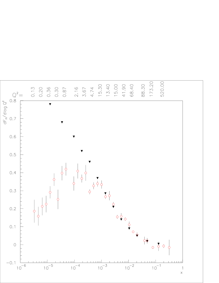
Figure 1: The HERA data and GRV’94 predictions (triangles) on the $F_{2}(x,Q^{2})$ slope. The data are taken from Ref.[2].

As can be seen, $\frac{\partial F_{2}}{\partial\ln Q^{2}}$ rises steeply with $\frac{1}{x}$ up to $x$ of approximately $5\times 10^{-3}$, for $Q^{2}\,>\,5\,{\,\mbox{GeV}^{2}}$. This is in agreement with the prediction of perturbative QCD   ( pQCD ) as manifested by the GRV’94 parameterization of $F_{2}(x,Q^{2})$. The data shows a dramatic departure from this prediction in the exceedingly small $x\,<\,5\times 10^{-3}$ and low $Q^{2}\,<\,5\,{\,\mbox{GeV}^{2}}$. In this kinematic domain, while GRV’94 predicts a continued increase of $\frac{\partial F_{2}}{\partial\ln Q^{2}}$ with $\frac{1}{x}$, the actual data indicates that the logarithmic $Q^{2}$ slope of $F_{2}$ decreases significantly with $\frac{1}{x}$, up to the present experimental limit of $x\,\simeq\,3\times 10^{-6}$.

There are some obvious experimental and theoretical observations and questions prompted by the above data:

1. What is the detailed $x$ and $Q^{2}$ dependence of $\frac{\partial F_{2}}{\partial\ln Q^{2}}$ ? As observed, the phenomenon of decreasing $\frac{\partial F_{2}}{\partial\ln Q^{2}}$ is associated with small $Q^{2}$ and exceedingly small $x$. However, since the data is so sparse it is difficult to deduce its detailed behaviour . In particular, the available data does not provide us with a clue as to the conduct of $\frac{\partial F_{2}}{\partial\ln Q^{2}}$ at medium and high $Q^{2}$, in the exceedingly small $x$ domain. Note, that the entire data sample with $x\,<\,5\times 10^{-3}$ has $Q^{2}$ values smaller than $5\,{\,\mbox{GeV}^{2}}$.

2. The experimental behaviour of $\frac{\partial F_{2}}{\partial\ln Q^{2}}$ as a function of $x$ and $Q^{2}$ shown in Fig.1, indicates a possible departure from the DGLAP pQCD behaviour of Eq. (1), for sufficiently small $x$. An interesting interpretation in this direction ( MRST ) has been recently proposed [5] assuming an initial “valence” gluon input distribution at small $Q^{2}$, which changes rapidly due to QCD evolution to the conventional “sea” distribution, at larger values of $Q^{2}$. We shall comment on this below.

   The experimental $F_{2}(x,Q^{2})$ data in the same kinematic region do not show any unconventional behaviour, i.e. $F_{2}$ is not sensitive enough, in the very small $x$ domain, to resolve new features. The new data suggest that the logarithmic $Q^{2}$ slope of $F_{2}$, is a more sensitive measure of possible deviations from the conventional pQCD dynamics.

3. The unexpected phenomenon occurs in the transition region between “hard” and “soft” physics and one should carefully assess our ability to understand it within the framework of pQCD. Specifically, the predominant “soft” inclusive total real photoproduction cross section is experimentally finite. Namely, the $Q^{2}=0$ limit of $\sigma_{tot}\,=\,\frac{4\pi^{2}\,\alpha_{em}}{Q^{2}}\,F_{2}(x,Q^{2})$ is finite at any $W$ and thus $F_{2}\,\,\propto\,\,Q^{2}$ as $Q^{2}\,\rightarrow\,0$. For a parameterization of the transition from DIS to real photoproduction, see Ref. [6]. However, the scale of this transition is not theoretically or experimentally specified. Generally, it is not clear if the observed change in the $x$ and $Q^{2}$ dependences of $\frac{\partial F_{2}}{\partial\ln Q^{2}}$ can be analyzed utilizing pQCD techniques, or if this is just a signature for the dominance of “soft” non perturbative physics, when both $Q^{2}$ and $x$ become small enough. Regardless, of its detailed dynamics, the data suggest a relatively smooth transition from the “hard” to the “soft” domains. Accordingly, we wish to match the “soft” ( non perturbative ) and the “hard” ( perturbative ) contributions probably around $Q^{2}\,\approx\,1-2\,{\,\mbox{GeV}^{2}}$, so as to better understand the “soft” limit of pQCD.

4. The theoretical interpretation of the new data presents a dual challenge . On one hand, it is desirable to understand and formulate the dynamics responsible for the changed behaviour of $\frac{\partial F_{2}}{\partial\ln Q^{2}}$, and to comprehend its implications for pQCD. On the other hand, regardless of this dynamics, the observed behaviour of $\frac{\partial F_{2}}{\partial\ln Q^{2}}$ implies that $xG(x,Q^{2})$ differs from our previous expectations in the limit of very small $x$ and $Q^{2}$. This is bound to impose changes on the input parton distributions which are currently used [4, 7, 8]. This is, indeed, the main point of Ref. [5].

5. An additional interesting study is to examine $\lambda\,=\,\frac{\partial\ln F_{2}}{\partial\ln(1/x)}$ from which one determines the dependence of $F_{2}$ as a power of $x$ at low $x$ and given $Q^{2}$, $F_{2}\,\propto\,x^{-\lambda(Q^{2})}$. $\lambda$ provides information pertinent to both Regge and pQCD analyses of $F_{2}$. As such we shall be interested in its $Q^{2}$ and $x$ dependences, and limits, and the constraints imposed on $\lambda$ by unitarity [9].

The goal of this paper is to expand and develop further the phenomenology and data analysis presented in our recent letter [10] in which the modified behaviour of $\frac{\partial F_{2}}{\partial\ln Q^{2}}$ was associated with the onset of unitarity screening corrections ( SC ).For an early suggestion that $\frac{\partial F_{2}}{\partial\ln Q^{2}}$ is sensitive to SC , see Ref. [11].

To this end we study below the $x$ and $Q^{2}$ behaviour of both $\frac{\partial F_{2}}{\partial\ln Q^{2}}$ and $\frac{\partial\ln F_{2}}{\partial\ln(1/x)}$, checking the applicability of pQCD in $x$ and $Q^{2}$ kinematic domains, not explored in detail previously.

A reliable execution of this program depends on our ability to compare our calculations with the relevant data. As noted, such data is available only at a few isolated values of averaged $x$ and $Q^{2}$. This limited data base is not sufficient to test our suggested phenomenology. To overcome this difficulty, we propose to use the ALLM’97 computer generated data base which we call “pseudo data ”. The ALLM parameterization [6] for the proton DIS structure function is a 23 parameter description which provides an excellent reproduction of the $\sigma_{tot}(\gamma^{*}p)$ data points. The updated fit [12] to 1356 data points with $0\,\leq\,Q^{2}\,\leq\,5000\,{\,\mbox{GeV}^{2}}$ and $3\times 10^{-6}\,<\,x\,<\,0.85$ yields a $\chi^{2}/ndf$ of 0.97. Notably, ALLM’97 reproduces well both the recent data on $\frac{\partial F_{2}}{\partial\ln Q^{2}}$ and $\frac{\partial\ln F_{2}}{\partial\ln(1/x)}$ (this is shown later in Fig.5b). As such, we assume that ALLM’97 provides an accurate and reliable reproduction of the data, against which we can assess our calculations and determine our free parameters.

The program of this paper is as follows: In Section II we briefly review the ALLM parameterization and its 1997 update. Section III is devoted to a theoretical review of the SC in hard parton physics and its relevance to $F_{2}$, $\frac{\partial F_{2}}{\partial\ln Q^{2}}$ and $\frac{\partial\ln F_{2}}{\partial\ln(1/x)}$ calculations. Our review examines the SC in the quark and gluon sectors. The systematics of $\frac{\partial F_{2}}{\partial\ln Q^{2}}$ and $\frac{\partial\ln F_{2}}{\partial\ln(1/x)}$ and its comparison to the pseudo data, defined above, are discussed in Section IV. Our summary and conclusions are given in Section V.

2 The ALLM’97 Pseudo Data Base:

The ALLM parameterization [6] was introduced in 1991 so as to reproduce $\sigma_{tot}(\gamma^{*}p)$, the total $\gamma^{*}p$ cross section above the resonance region, for a very wide $Q^{2}$ range including real photoproduction ( $Q^{2}=0$ ). This is a multiparameter fit ( 23 parameters ) to all available data on $\sigma_{tot}(\gamma p)$ and $F_{2}$, based on a Regge - type approach formulated so as to be compatible with pQCD and the DGLAP evolution equations. In its latest 1997 update [12] a fit was performed to 1356 data points [1, 13], for which an excellent $\chi^{2}/ndf$ = 0.97 was obtained.

The ability to reproduce $\sigma_{tot}(\gamma^{*}p)$ over a wide kinematic range of $3\times 10^{-6}\,<\,x\,<\,0.85$ and $0\,\leq\,Q^{2}\,\leq\,5000\,{\,\mbox{GeV}^{2}}$, is further demonstrated by the success of ALLM’97 in fitting the $F_{2}$ logarithmic slopes, $\frac{\partial F_{2}}{\partial\ln Q^{2}}$ and $\frac{\partial\ln F_{2}}{\partial\ln(1/x)}$ well. This is of particular interest, as the parameterization reproduces the $F_{2}$ and its logarithmic derivative data, also in the limit of exceedingly small $x\,<\,5\times 10^{-3}$.

The ALLM parameterization is presented by the following equations:

$$F_{2}(x,Q^{2})\,\,\,=\,\,\,\frac{Q^{2}}{Q^{2}\,+\,m^{2}_{0}}\,\left(\,F^{P}_{2}(x,Q^{2})\,\,+\,\,F^{R}_{2}(x,Q^{2})\,\right)\,\,,$$ (2)

where $F^{P}_{2}$ and $F^{R}_{2}$ are the respective contributions of the Pomeron and the secondary Reggeon exchanges to $F_{2}$.

$$F^{P}_{2}(x,Q^{2})\,\,\,=\,\,\,C_{P}(\tau)(\,\frac{1}{x_{P}}\,)^{\alpha_{P}(\tau)\,-\,1}\,(\,1\,-\,x\,)^{\beta_{P}(\tau)}\,\,;$$ (3)

$$F^{R}_{2}(x,Q^{2})\,\,\,=\,\,\,C_{R}(\tau)(\,\frac{1}{x_{R}}\,)^{\alpha_{R}(\tau)\,-\,1}\,(\,1\,-\,x\,)^{\beta_{R}(\tau)}\,\,;$$ (4)

where $\tau\,\,=\,\,\ln\left(\frac{\ln\frac{Q^{2}+Q^{2}_{0}}{\Lambda^{2}}}{\ln\frac{Q^{2}_{0}}{\Lambda^{2}}}\right)$ is a slowly varying variable.

The two modified Bjorken $x$ - variables are defined

$$\frac{1}{x_{P}}\,\,\,=\,\,\,1\,\,+\,\,\frac{W^{2}-M^{2}}{Q^{2}\,+\,m^{2}_{P}}\,\,;$$ (5)

$$\frac{1}{x_{R}}\,\,\,=\,\,\,1\,\,+\,\,\frac{W^{2}-M^{2}}{Q^{2}\,+\,m^{2}_{R}}\,\,.$$ (6)

$M$ denotes the proton mass and $m_{P}$ and $m_{R}$ are fitted effective Pomeron and Reggeon scales. The scale parameters $m^{2}_{0}$, $m^{2}_{P}$, $m^{2}_{R}$ and $Q^{2}_{0}$ control the smooth transition from $Q^{2}=0$ to high $Q^{2}$. When $Q^{2}\,\gg\,m^{2}_{P}$ and $m^{2}_{R}$, $x_{P}$ and $x_{R}$ approach $x$. $C_{R}$, $\alpha_{R}$, $\beta_{R}$ and $\beta_{P}$ increase with $Q^{2}$ as

$$f(\tau)\,\,=\,\,f_{1}\,\,+\,\,f_{2}\,\tau^{f_{3}}\,\,$$ (7)

whereas $C_{P}$ and $\alpha_{P}$ decrease with $Q^{2}$ as

$$g(\tau)\,\,=\,\,g_{1}\,\,+\,\,(\,g_{1}\,\,-\,\,g_{2}\,)\,[\,\frac{1}{1\,+\,\tau^{g_{3}}}\,\,-\,\,1\,]\,\,.$$ (8)

The parameterization depends on 23 parameters which are determined from the data fit. About half of these parameters are required to describe the low $W$ ( high $x$ ) region where higher QCD twist terms are important. A specification of the ALLM’97 fitted parameters is given in Table 2 of Ref. [12].

In general, Eqs. (3) and (4) were constructed to be compatible with pQCD and reproduce two limiting cases:

(i) Reggeon - like behaviour at $x\,\,\rightarrow\,0$, with all corrections to the simple one Reggeon exchange absorbed in the dependence of the Reggeon intercept on $\tau$ .

(ii) The pQCD quark counting rules behaviour at $x\,\rightarrow\,1$, for which the power dependence of $\beta_{P}$ and $\beta_{R}$ on $\tau$ are expected.

In as much as the ALLM parameterization is constructed in a Regge-like scheme, it is important to note, that it is not a theory to be compared with the data, but a parameterization aimed at the best possible reproduction of the data. The ALLM’97 parameters have two basic features dictated by the data, but not expected in a simple Regge-like theory.

1) The Pomeron has a high scale of $m^{2}_{P}\,\simeq\,50\,{\,\mbox{GeV}^{2}}$. This high value is necessary to maintain a very smooth transition from predominantly “soft” $Q^{2}\,=\,0$ to a predominantly “hard” $Q^{2}$ of a few ${\,\mbox{GeV}^{2}}$. A smaller value of $m^{2}_{P}\,\simeq\,10\,{\,\mbox{GeV}^{2}}$, suggested in the original ALLM fit [6], implies a very fast transition, which is not compatible with the new data.

2) Theoretically, for a single Reggeon exchange, $\alpha_{R}$ should be independent of $Q^{2}$. The $Q^{2}$ dependence, implied by the ALLM parameterization, secures the reproduction of the DIS data, indicating the need to correct the simple Regge picture in DIS.

In this paper we evaluate the logarithmic derivatives $\frac{\partial F_{2}}{\partial\ln Q^{2}}$ and $\frac{\partial\ln F_{2}}{\partial\ln(1/x)}$ derived from ALLM , Eq. (2) - Eq. (8). The calculated $\frac{\partial F_{2}}{\partial\ln Q^{2}}$ and $\frac{\partial\ln F_{2}}{\partial\ln(1/x)}$ coincide with the experimental data in the kinematic region where they were measured. The ability to produce this detailed pseudo data base enables us to achieve two goals:

1. To achieve a realistic reproduction of the behaviour of $\frac{\partial F_{2}}{\partial\ln Q^{2}}$ and $\frac{\partial\ln F_{2}}{\partial\ln(1/x)}$, over the complete $Q^{2}$ range, with a special emphasis on the small $Q^{2}$ and exceedingly small $x$ domain.

2. In our search for a dynamical explanation for possible deviations from the DGLAP pQCD expectations, we offer in section IV a pQCD calculation modified by SC which reproduces both the real data and the pseudo data points for $Q^{2}\,>\,0.4\,{\,\mbox{GeV}^{2}}$, as well as .

A presentation and discussion of these issues will be given in section IV.

An important item concerning ALLM is the uncertainty of the fit. An error calculation of a 23 parameter fit,where many of the parameters are highly correlated, is non trivial. Based on the estimates of Ref.[6], we assess the pseudo data errors to be approximately 8 - 10% . Over the kinematic region of interest the ALLM calculated errors are smaller than the comparable experimental errors. In section IV, which is devoted to the data analysis including the ALLM’97 pseudo data, we quote both errors whenever possible.

3 The Calculation of $\mathbf{F}_{2}$ slopes with SC

As stated in Ref.[10], we claim that a calculation of $\frac{\partial F_{2}}{\partial\ln Q^{2}}$ including SC effects accounts well for the data shown in Fig.1.

In the SC calculation we distinguish between two contributions leading to observed deviations from the DGLAP predictions of Eq. (1). These are:

1. SC in the quark sector, corresponding to the passage of a $q\bar{q}$ pair through the target .

2. The analogous SC in the gluon sector, as $xG(x,Q^{2})$ appears in the expression for the slope of $F_{2}$, Eq. (1).

3.1 Screening in the quark sector

SC in the quark sector, calculated in the Eikonal approximation, were derived some time ago [14] [15] leading to an extensive phenomenology [16]. In our context we have

$$\displaystyle{\frac{\partial F^{SC}_{2}(x,Q^{2})}{\partial\ln(Q^{2}/Q^{2}_{0})}} = \displaystyle{\frac{Q^{2}}{3\,\pi^{2}}\,\int db^{2}_{t}\,\,\{\,\,1\,\,\,-\,\,\,e^{-\kappa_{Q}(x,Q^{2};b^{2}_{t})}\,\,\}\,\,;}$$ (9)

$$\displaystyle{\kappa_{Q}(x,Q^{2};b^{2}_{t})} = \displaystyle{\frac{2\pi\alpha_{\rm S}}{3\,Q^{2}}\,\Gamma(b_{t})\,\,xG^{\mbox{\scriptsize DGLAP}}(x,Q^{2})}$$ (10)

$Q^{2}_{0}$ is the photon virtuality scale from which we start the DGLAP evolution. $\Gamma(b_{t})$ is the two gluon non-perturbative form factor of the target in impact parameter representation.

$$\Gamma(b_{t})\,\,=\,\,\frac{1}{\pi}\,\,\int\,e^{-i(\vec{b}_{t}\cdot\vec{q}_{t})}\,F(t)\,d^{2}q_{t}$$ (11)

with $t=-q^{2}_{t}$ and $F(t)$ denoting the form factor in $t$ - representation.

The fact that the $b_{t}$- dependence factorizes from the $x$ and $Q^{2}$ dependences was shown in Ref. [17] from the DGLAP evolution equations, using the factorization theorem [18]. It should be stressed that the factorization we use in Eq. (10) is only valid for $t\,\leq\,Q^{2}_{0}$. Therefore, we assume below that only such small values of $t$ are important in our integrals. This is the justification for simplifying the $b_{t}$-dependence of Eq. (11), and using a Gaussian parameterization for $\Gamma(b_{t})$:

$$\Gamma(b_{t})\,\,=\,\,\frac{1}{R^{2}}\,e^{-\frac{b^{2}_{t}}{R^{2}}}\,\,.$$ (12)

where $R^{2}$ is a fitted parameter.

Figure 2: The first order SC $\propto\,\kappa^{2}$ for $F_{2}(x,Q^{2})$.

In Fig.2 we present the lowest order SC to $F_{2}$ which are proportional to $\kappa^{2}_{Q}$, within the framework of the additive quark model ( AQM ) ( see Eq. (9) ). In the AQM we distinguish between two typical scales in the integration over $q_{t}$. In the first diagram of Fig.2 we integrate over the distance between two constituent nucleon quarks. In the second diagram of Fig.2 the relevant integration is over the size of the constituent quark ( see Refs. [19] [20] ). Eq. (9) assumes that the only constraint on the two gluons is their confinement within a nucleon whose size is $R$.

The important property of Eq. (9) is that the calculated SC in the quark sector depends on a distance $r^{2}_{\perp}\,\,=\,\,\frac{4}{Q^{2}}$ which we consider to be short enough for all values of $Q^{2}$ in our calculation. Consequently, we assess the perturbative calculation of the SC for $\frac{\partial F_{2}(x,Q^{2})}{\partial\ln(Q^{2}/Q^{2}_{0})}$ to be reliable. This is not so for the calculation of the SC for $F_{2}$, which has an important contribution from large distances $r^{2}_{\perp}\,>\,\frac{4}{Q^{2}}$ as will be discussed below. As a result, the calculations of SC for $F_{2}$ are not that well defined, and may contain arbitrary errors.

Following our previous publications [10, 21], we define a damping factor

$$D^{2}_{Q}(\kappa)\,\,=\,\,\frac{\frac{\partial F^{SC}_{2}(x,Q^{2})}{\partial\ln(Q^{2}/Q^{2}_{0})}}{\frac{\partial F^{\mbox{\scriptsize DGLAP}}_{2}(x,Q^{2})}{\partial\ln Q^{2}}}\,\,,$$ (13)

where $\frac{\partial F^{SC}_{2}(x,Q^{2})}{\partial\ln(Q^{2}/Q^{2}_{0})}$ is calculated from Eq. (9). The behaviour of $D^{2}_{Q}(\kappa)$ as a function of $x$ and $Q^{2}$ is plotted in Fig.3a  , where we take $R^{2}\,=\,10\,GeV^{-2}$.

3.2 Screening in the gluon sector

The calculation of the SC in the gluon sector using an Eikonal approach was derived by Mueller [15] and further discussed in Ref.[22]. We obtain

$$xG^{SC}(x,Q^{2})\,\,=\,\,\frac{2}{\pi^{2}}\,\int^{1}_{x}\,\frac{dx^{\prime}}{x^{\prime}}\,\int^{Q^{2}}_{Q^{2}_{0}}\,dQ^{\prime 2}\,\int db^{2}_{t}\,\,\{\,\,1\,\,\,-\,\,\,e^{-\kappa_{G}(x^{\prime},Q^{\prime 2};b^{2}_{t})}\,\,\}\,\,+\,\,xG(x,Q^{2}_{0})\,\,.$$ (14)

Note that $\kappa_{G}(x^{\prime},Q^{\prime 2},b^{2}_{t})\,\,=\,\,\frac{9}{4}\kappa_{Q}(x^{\prime},Q^{\prime 2},b^{2}_{t})$ defined in Eq. (10).

We can now define a gluon damping factor

$$D^{2}_{G}(x,Q^{2})\,=\,\frac{xG^{SC}(x,Q^{2})}{xG^{\mbox{\scriptsize DGLAP}}(x,Q^{2})}\,\,,$$ (15)

where $xG^{SC}(x,Q^{2})$ is calculated from Eq. (14).

A difficulty in our calculation stems from the fact that the $Q^{\prime 2}$ integration spans not only the short ( perturbative ), but also the long ( non-perturbative ) distances. Lacking solid theoretical estimates, we suppress the long distance contributions to Eq. (14) by imposing a cutoff on the $Q^{\prime 2}$ integration, so as to neglect the contributions from $r_{\perp}\,>\,\frac{1}{Q_{0}}$ integration. This ad hoc procedure makes our estimate of $D^{2}_{G}(x,Q^{2})$ less reliable than the $D^{2}_{Q}(x,Q^{2})$ estimate. We have checked our cutoff procedure at $Q^{2}_{0}\,=\,1\,{\,\mbox{GeV}^{2}}$, using the GRV’94 parameterization for the solution of the DGLAP evolution equations and putting $xG(x,Q^{2})=0$ for $Q^{2}<Q^{2}_{0}$ ( we shall denote this model GLMN0 ) or imposing the GRV initial condition for $xG(x,Q^{2})$ at $Q^{2}=Q^{2}_{0}$ ( GLMN1 ). The output result for $D^{2}_{G}(x,Q^{2})$ differs by about 10%, which lends credibility to our calculation. A graphical representation of $D^{2}_{G}$ is provided in Fig.3b  . Note that $D^{2}_{G}$ is consistently smaller than $D^{2}_{Q}$, i.e. SC in the gluon sector are bigger than the SC in the quark sector. We also observe that for any $Q^{2}$ the overall damping $D_{Q}^{2}\!\cdot\!D_{G}^{2}$ becomes significant once $x$ is small enough.

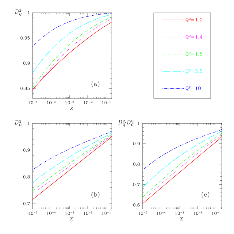
Figure 3: The damping factors: (a) $D^{2}_{Q}(x,Q^{2})$, (b) $D^{2}_{G}(x,Q^{2})$ and
(c) $D^{2}_{Q}(x,Q^{2})\!\cdot\!D^{2}_{G}(x,Q^{2})$.

To check our sensitivity to the region of low $Q^{\prime 2}$ we use a general property of the gluon structure function, namely, that gauge invariance requires that $xG\,\propto\,Q^{2}$ at low $Q^{2}$    ( see Ref.[23] for discussion ).    Relying on this general property we assume that

$$xG\left(x,Q^{2}<\mu^{2}\right)=\frac{Q^{2}}{\mu^{2}}xG\left(x,\mu^{2}\right)\,,$$ (16)

where $\mu^{2}$ is a free parameter in the range $0.4\,\,\leq\,\,\mu^{2}\,\,\leq\,\,1\,\,{\,\mbox{GeV}^{2}}$. We are motivated by the observation that even though GRV’94 evolves from a very low $Q^{2}_{0}\,=\,0.4\,{\,\mbox{GeV}^{2}}$, they actually fit the $F_{2}$ data only above $Q^{2}$ of about $1\,{\,\mbox{GeV}^{2}}$. We have satisfied ourselves that our calculations are stable ( within 10$\%$ ) to the choice of $\mu^{2}$.

3.3 Overall screening

Our final expression for $\frac{\partial F_{2}(x,Q^{2})}{\partial\ln(Q^{2}/Q^{2}_{0})}$, i.e. the $Q^{2}$ logarithmic slope of $F_{2}$ with SC included in the calculation, is

$$\frac{\partial F^{SC}_{2}(x,Q^{2})}{\partial\ln(Q^{2}/Q^{2}_{0})}\,\,=\,\,D^{2}_{Q}(x,Q^{2})\,D^{2}_{G}(x,Q^{2})\,\frac{\partial F^{\mbox{\scriptsize DGLAP}}_{2}(x,Q^{2})}{\partial\ln(Q^{2}/Q^{2}_{0})}\,\,.$$ (17)

A detailed analysis of the systematics emerging from the above formula is given in the next section.

The choice of input parton distributions obviously influences the output. At first sight, we have a very clear prescription of what to do. Indeed, the DGLAP evolution equations as well as our Eq. (9) and Eq. (14) ( see also the full set of equations below, Eq. (18) - Eq. (22), where the initial parton distributions are noted explicitly ) are written in such a way that we depend on the initial parton distributions at a fixed $Q^{2}=Q^{2}_{0}$, to solve them. These initial distributions, in principle, include everything that we have from “soft”, non-perturbative physics. All the information relevant to short distances $r_{\perp}\,<\,\frac{1}{Q_{0}}$ is included in the above equations both with or without SC.

In an ideal situation, our procedure should be to use as input a set of parton distributions which have been determined at $Q^{2}=Q^{2}_{0}$, without the influence of data at $Q^{2}\,>\,Q^{2}_{0}$, evolve to higher $Q^{2}$ using DGLAP evolution, and then correct for SC at $Q^{2}\,>\,Q^{2}_{0}$, utilizing the damping factors.

Unfortunately, such a set of input parton structure functions is not available, and we must make do with one of the available parameterization. These sets are obtained from global fits combined with DGLAP evolution equations, i.e. the determination of the input is also influenced by the data with $Q^{2}\,>\,Q^{2}_{0}$ which may contain SC. We have chosen to work with GRV’94 parameterization since this is a relatively old parameterization and as such most of the fitted data has $x>10^{-3}$. Our estimates show that in this kinematic region we expect the SC to be small.

The GRV’94 parameterization has an additional advantage for us. It should be stressed that Eq. (9), Eq. (14) and Eqs. (18)–(22) in the following are proven in the double log approximation ( DLA ) in which we consider both $\alpha_{\rm S}\,\ln(1/x)\,>\,1$ and $\alpha_{\rm S}\,\ln(Q^{2}/Q^{2}_{0})\,>\,1$. In the GRV’94 parameterization the initial value of $Q^{2}_{0}\,=\,0.4{\,\mbox{GeV}^{2}}$ is so small, that the DLA is effectively valid above $Q^{2}\,\,\approx\,\,1{\,\mbox{GeV}^{2}}$. Indeed, above $1{\,\mbox{GeV}^{2}}$ GRV’94 provides a good reproduction of the DIS data.

In a previous publication [20] we have discussed the possibility that the proton is better described as a two radii object. This description is based on the large experimental difference between the slopes in $\frac{d\sigma}{dt}$ of $\gamma p\,\rightarrow\,J/\Psi p$ and $\gamma p\,\rightarrow\,J/\Psi X$. We have formulated this option in Ref. [20] and have applied it to $\frac{\partial F^{SC}_{2}(x,Q^{2})}{\partial\ln(Q^{2}/Q^{2}_{0})}$ in Ref. [10] in which both a single and two radii models of the proton were examined. In as much as we endorse the two radii idea, we are unable, at this stage, to offer a decisive experimental signature that will discriminate between the one and two radii models ,when dealing with $F_{2}$ and its logarithmic slopes. This being the case, we limit ourselves in this paper to the simpler one radius approach. A detailed formalism for the two radii model was given in Refs. [20] and [10].

3.4 A screened calculation for $\mathbf{\lambda}(Q^{2})$

We list below the expressions for $F^{SC}_{2}(x,Q^{2})$ and $\lambda(Q^{2})\,=\,\frac{\partial\ln F^{SC}_{2}(x,Q^{2})}{\partial\ln(1/x)}$ which include screening corrections. The set of formulae are :

$$F^{SC}_{2}(x,Q^{2}) = \frac{R^{2}\,N_{c}}{2\,\pi^{2}}\,\sum^{N_{f}}_{f=1}\,Z^{2}_{f}\,\,\int^{Q^{2}}_{Q^{2}_{0}}\,dQ^{\prime 2}\,\left\{\,C\,+\,\ln\kappa^{SC}_{Q}(x,Q^{\prime 2})\,+\,E_{1}\left(\kappa^{SC}_{Q}(x,Q^{\prime 2})\right)\,\right\}$$ (18)

$$\mbox{}+F^{\mbox{\scriptsize input}}_{2}(x,Q^{2}_{0})\,\,;$$

$$\frac{\partial F^{SC}_{2}(x,Q^{2})}{\partial\ln(1/x)} = \frac{R^{2}\,N_{c}}{2\,\pi^{2}}\,\sum^{N_{f}}_{f=1}\,Z^{2}_{f}\,\,\int^{Q^{2}}_{Q^{2}_{0}}\,dQ^{\prime 2}\,\frac{\partial\ln\left(xG^{SC}\left(x,Q^{\prime 2}\right)\right)}{\partial\ln(1/x)}\,\left\{\,1\,\,-\,\,e^{-\kappa^{SC}_{Q}(x,Q^{\prime 2})}\,\right\}$$ (19)

$$\mbox{}+\frac{\partial F^{\mbox{\scriptsize input}}_{2}(x,Q^{2}_{0})}{\partial\ln(1/x)}\,\,;$$

$$\kappa^{SC}_{Q}(x,Q^{2}) = \frac{2\,\pi\,\alpha_{\rm S}\left(Q^{2}\right)}{3\,R^{2}\,Q^{2}}\,xG^{SC}(x,Q^{2})\,\,;$$ (20)

$$xG^{SC}\left(x,Q^{2}\right) = \frac{2\,R^{2}}{\pi^{2}}\,\int^{1}_{x}\,\frac{dx^{\prime}}{x^{\prime}}\,\int^{Q^{2}}_{Q^{2}_{0}}\,d\,Q^{\prime 2}\,\left\{\,C\,+\,\ln\kappa^{\mbox{\scriptsize DGLAP}}_{G}(x^{\prime},Q^{\prime 2})\,+\,E_{1}\left(\kappa^{\mbox{\scriptsize DGLAP}}_{G}(x^{\prime},Q^{\prime 2})\right)\,\right\}$$ (21)

$$\mbox{}+xG^{\mbox{\scriptsize input}}(x,Q^{2}_{0})\,\,;$$

$$\kappa^{\mbox{\scriptsize DGLAP}}_{G}(x,Q^{2}) = \frac{3\,\pi\,\alpha_{\rm S}\left(Q^{2}\right)}{2\,R^{2}\,Q^{2}}\,xG^{\mbox{\scriptsize DGLAP}}(x,Q^{2})\,\,.$$ (22)

We have to integrate over the all distances including the long distance region. As we have discussed, this gives rise to undefined errors in our calculation which we attempt to estimate, assuming different cutoff values of the distances $r_{\perp}\,\,>\,\,\frac{1}{Q_{0}}$. All integrals over the impact parameter $b_{t}$, were done using the Gaussian parameterization for the $b_{t}$ dependence of Eq. (12). In the above set of equations $C$ denotes the Euler constant ( $C\,=\,0.577$ ) and $E_{1}(x)\,=\,-Ei(-x)$ is the exponential integral function (see Ref. [24]). $N_{c}$ and $N_{f}$ are the colour and flavour degrees of freedom in QCD. $Z_{f}$ is the fraction of the electrical charge carried by a quark with flavor $f$.

3.5 Asymptotic predictions

It is instructive to discuss here the asymptotic predictions of Eq. (9)  - Eq. (22) in the region of very small $x$. Such predictions have been discussed previously ( see Refs. [10, 15, 19, 25] ) and we consider them here as a limit with which we can compare our actual calculations.

In the region of small $x$, which is defined in our formulae as a region where

$$\kappa^{\mbox{\scriptsize DGLAP}}_{Q}(x,Q^{2})\,\,=\,\,\frac{2\,\pi\,\alpha_{\rm S}(Q^{2})}{3\,R^{2}\,Q^{2}}\,xG^{\mbox{\scriptsize DGLAP}}(x,Q^{2})\,\,>\,\,1\,\,,$$ (23)

the predictions for all observables which we discuss in this paper are as follows:

1. $F^{SC}_{2}(x,Q^{2})\,\,\Longrightarrow\,\,\frac{N_{c}}{2\pi^{2}}\,\sum^{N_{f}}_{1}\,Z^{2}_{f}\,Q^{2}\,R^{2}\,\ln\kappa_{Q}(x,Q^{2})\,\,;$

2. $\frac{\partial F^{SC}_{2}(x,Q^{2})}{\partial\ln(Q^{2}/Q^{2}_{0})}\,\,\propto\,\,R^{2}Q^{2}$ for $x\,\leq\,x_{0}$, where $x_{0}$ is determined from the equation:

   $\kappa^{\mbox{\scriptsize DGLAP}}_{G}(x_{0},Q^{2})\,=\,1\,\,.$ The solution to the equation $\kappa^{\mbox{\scriptsize DGLAP}}_{G}(x,Q^{2})\,=\,1$ is plotted in Fig.4, where we plot also the solutions for $\kappa^{\mbox{\scriptsize DGLAP}}_{G}\,=$ 0.5 and 1.5.

   It should be stressed that at any value of $Q^{2}$, for very small $x\,<\,x_{0}$ , the limit of the $F_{2}$ slope $\frac{\partial F^{SC}_{2}(x,Q^{2})}{\partial\ln(Q^{2}/Q^{2}_{0})}$ is independent of $x$, and is proportional to $Q^{2}$.

   

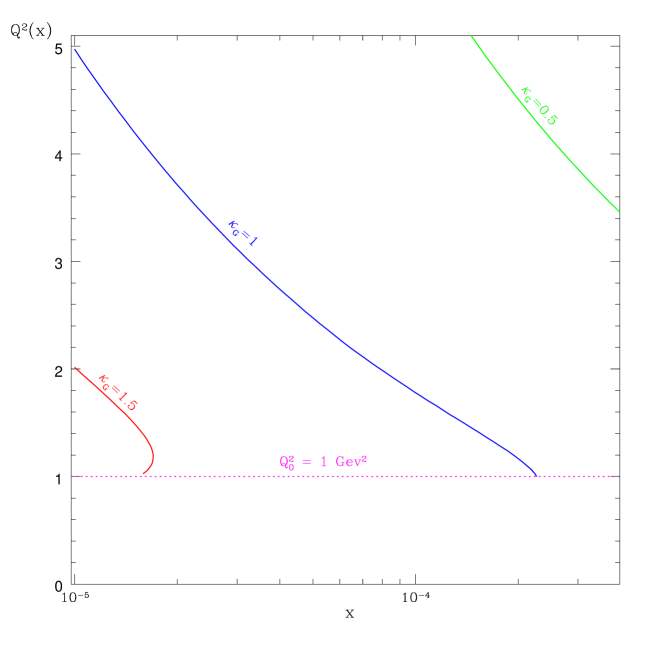
   Figure 4: Solutions to $\kappa_{G}\,=$ 0.5, 1 and 1.5.

   This limiting behaviour is reached at smaller and smaller $x$ values as $Q^{2}$ is increased, and it may explain the $Q^{2}$ - dependence of the experimental data ( see Fig.1 )  ;

3. $\frac{\partial\ln F^{SC}_{2}(x,Q^{2})}{\partial\ln(1/x)}\,\,\propto\,\,\frac{1}{\ln(1/x)\,\ln\ln(1/x)}$ . Therefore, in the region of ultra small $x$:   $\lambda(Q^{2})\,=\,\frac{\partial\ln F^{SC}_{2}(x,Q^{2})}{\partial\ln(1/x)}\,\,\Longrightarrow\,\,0$, modulo logarithmic corrections independent of the value of $Q^{2}$. We shall elaborate on this limiting behaviour in the next section  ;

4. $xG^{SC}(x,Q^{2})\,\,\Longrightarrow\,\,\frac{2\,R^{2}\,Q^{2}}{\pi^{2}}\,\ln(1/x)\,\ln\kappa_{G}^{\mbox{\scriptsize DGLAP}}(x,Q^{2})$. Comparing this behaviour of the gluon structure function with the asymptotic behaviour of $\frac{\partial F^{SC}_{2}(x,Q^{2})}{\partial\ln(Q^{2}/Q^{2}_{0})}$ one can deduce that Eq. (1) does not hold in the region of exceedingly small $x$.

Obviously, the above are just the exceedingly small $x$ limits of the actual expressions, but they give us, together with the DGLAP predictions, a framework to discuss the experimental results, so as to develop a strategy of measurement which can test the asymptotic predictions.

4 Comparison with the experimental results
and pseudo data

The calculations presented in this paper were carried out with $R^{2}\,=\,10\,{\,\mbox{GeV}^{2}}$ and $Q^{2}_{0}\,=\,0.4\,{\,\mbox{GeV}^{2}}$. We have not attempted to produce a “best fit”. However, we have satisfied ourselves that with these input parameters, we obtain good results which provide a consistent reproduction of the measured and pseudo data. As stated, we have not pursued further the study of a two radii model [10] [20] being unable to suggest a decisive signature which supports this hypothesis.

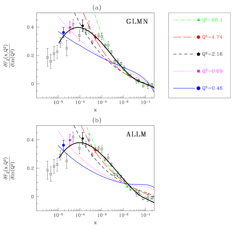
Figure 5: (a) Our calculations for ZEUS data. The thick line is the prediction for the actual ZEUS data which were taken at values of $Q^{2}$ correlated with the value of $x$. (b) The same with ALLM’97 .

The detailed features of our reconstruction of the ZEUS data [2] are shown in Fig.5a. As noted, the confusing compilation of experimental data points with widely spread ($x,Q^{2}$) values presented in this figure, makes it difficult to directly assess the $x$ dependence of $\frac{\partial F_{2}(x,Q^{2})}{\partial\ln(Q^{2}/Q^{2}_{0})}$ at a fixed $Q^{2}$. Our analysis suggests that $\frac{\partial F_{2}(x,Q^{2})}{\partial\ln(Q^{2}/Q^{2}_{0})}$ grows monotonically with $\frac{1}{x}$ at fixed $Q^{2}$, approaching its limiting value at $x$ which is well below the $x$ interval valid in our calculations. At high $Q^{2}$ and at fixed $x$, this rise is steep following the behaviour of $xG^{\mbox{\scriptsize DGLAP}}(x,Q^{2})$ as expected from Eq. (1). In our approach, this is a direct consequence of the fact that in the high $Q^{2}$ limit and at fixed $x$, $D^{2}_{Q}\,\,\approx\,\,D^{2}_{G}\,\,\approx\,\,1$ throughout the $x$ range of interest. Generally, for any fixed $Q^{2}$ we can find $x_{0}$ sufficiently small so that for $x\,<\,x_{0}$ SC are important and, thus, both $D^{2}_{Q}$ and $D^{2}_{G}$ are significantly smaller than 1. However, from a practical point of view, as data are available for $x\,>\,2\times 10^{-6}$ and the GRV’94 parameterization is defined for $x\,>\,10^{-5}$, SC become relevant only at moderate and small $Q^{2}$ values ( see Fig.3 ). This general behaviour is reflected in our calculations where $\frac{\partial F^{SC}_{2}(x,Q^{2})}{\partial\ln(Q^{2}/Q^{2}_{0})}$ departs from the DGLAP predictions, and as $Q^{2}$ decreases the $x$ dependence of $\frac{\partial F^{SC}_{2}(x,Q^{2})}{\partial\ln(Q^{2}/Q^{2}_{0})}$ becomes more moderate. Note that our approximations are not valid for $x\,>\,10^{-1}$ values. The final compilation of the calculated points, at $(x,Q^{2})$ values matching the experimental ones, reproduces the data very well, as is evident from the thick line of Fig.5a. The other lines in Fig.5a are for five typical constant $Q^{2}$ values, selected from the experimental data. Note that the thick curve in the figure, like the data points, belong to different $Q^{2}$ values.

In Fig. 5b we show the same plot as in Fig.5a, only this time the fixed $Q^{2}$ behaviour is determined from ALLM’97 [12]. Evidently, the behaviour of $\frac{\partial F_{2}(x,Q^{2})}{\partial\ln(Q^{2}/Q^{2}_{0})}$, at fixed $Q^{2}$, shown in Fig.5b is very close to our calculated behaviour presented in Fig.5a.

Assuming the ALLM’97 pseudo data to be a reliable reproduction of the, unmeasured yet, real data - we can assess the various theoretical ideas and predictions for $\frac{\partial F_{2}(x,Q^{2})}{\partial\ln Q^{2}}$, which are compared with the pseudo data in Figs 6 and 7.

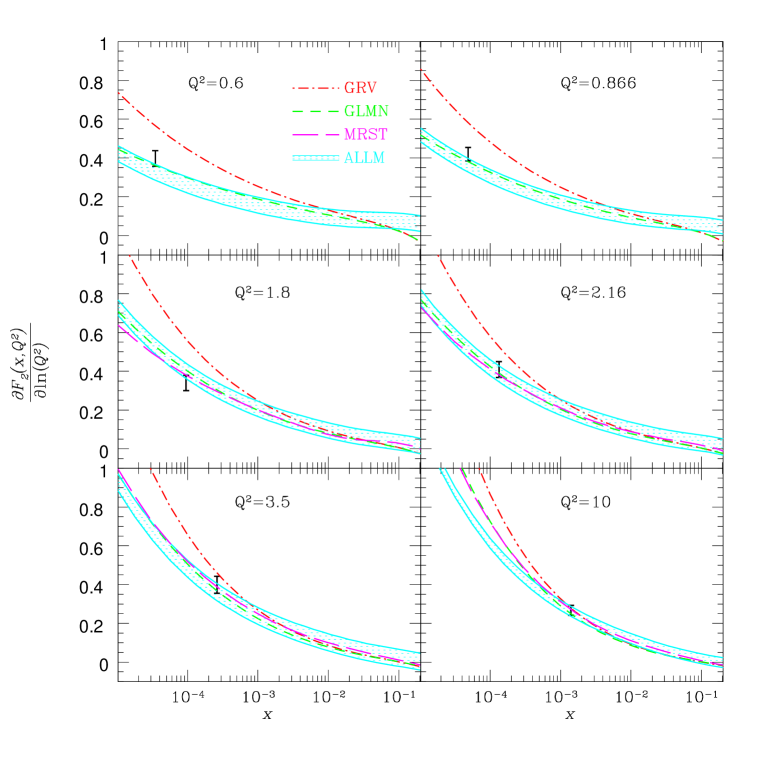
Figure 6: $\frac{\partial F_{2}(x,Q^{2})}{\partial\ln Q^{2}}$ at fixed $Q^{2}$. In addition to the ALLM band we show a typical data point with its error

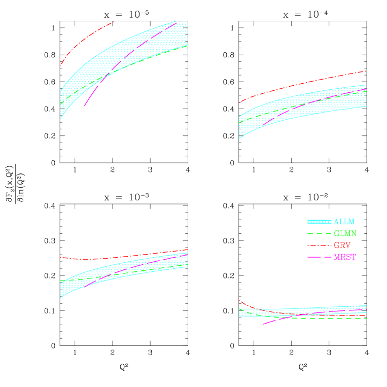
Figure 7: $\frac{\partial F_{2}(x,Q^{2})}{\partial\ln Q^{2}}$ at fixed $x$.

A detailed comparison between ALLM’97 and the results obtained from our calculation ( GLMN ) as well as GRV’94 [4] and MRST [5] are presented in Fig.6 for various $Q^{2}$ values. ALLM’97 is presented as a band which includes the estimated error [6]. We also show the typical small $x$ experimental errors, so as to better assess the quality of the theoretical predictions. In Fig.7 we compare the pseudo data $Q^{2}$ dependence of $\frac{\partial F_{2}(x,Q^{2})}{\partial\ln Q^{2}}$ at fixed $x$ values of $10^{-2}$, $10^{-3},\,10^{-4}$ and $10^{-5}$ with the same parameterizations, and the results of our calculation. Note that the MRST [5] parameterization is valid only for $Q^{2}\,>\,1.25\,{\,\mbox{GeV}^{2}}$.

1. Figs.5 - 7 show that the SC are able to account for the deviations from the DGLAP prediction, observed experimentally and reproduced in the ALLM’97 pseudo data. Our calculations are compatible with the observable scale $Q^{2}\,\approx\,2-4\,{\,\mbox{GeV}^{2}}$ where such deviations start to be visible.

2. In our approach we do not see any indication supporting an abrupt transition from the predominantly “soft” region to the hard one. This is compatible with the ALLM’97 fit which had to choose a high Pomeron mass scale $m^{2}_{P}\,\approx\,50\,{\,\mbox{GeV}^{2}}$, so as to obtain a very gradual increase of the effective $\alpha_{P}(0)$, with increasing $Q^{2}$ as required by the data.

3. Figs.5 - 7 are compatible with a new scale of hardness ( $Q^{2}(x)$ ) suggested in our main formulae ( Eq. (18) - Eq. (22) ). $Q^{2}(x)$ is the solution of the equation

   $$\kappa^{\mbox{\scriptsize DGLAP}}_{G}(x,Q^{2}(x))\,=\,1\,\,.$$ (24)

   The general features of this equation are shown in Fig.4, where the relevant $Q(x)$ values can be identified. The novelty of this approach is that a hardness scale is derived for any $x$ value under consideration.

Comparing GLMN with GRV’94 and MRST we observed that both GLMN and MRST are significantly different from GRV’94 in accord with the real and pseudo data. We note also that in the exceedingly small $x\approx 10^{-5}$ region the $Q^{2}$ dependence of MRST becomes different from ours but we are unable, at this stage, to check it experimentally.

A summary of the $Q^{2}$ dependence of $\lambda(Q^{2})\,\,=\,\,\frac{\partial\ln F_{2}(x,Q^{2})}{\partial\ln(1/x)}$ at fixed $x$ values of $10^{-5},\,10^{-4}$ and $5\times 10^{-3}$ is presented in Fig.8, where, once again, the ALLM’97 pseudo data is compared with the GRV’94 and MRST parameterizations and our results. The GLMN calculation was carried out with $\mu^{2}\,=\,0.6\,{\,\mbox{GeV}^{2}}$ controlling our continuation to very small $Q^{2}\,<\,0.6\,{\,\mbox{GeV}^{2}}$, where $xG(x,Q^{2}<\mu^{2})\,=\,\frac{Q^{2}}{\mu^{2}}xG(x,\mu^{2})$. To check our sensitivity we plot in Fig.9 the results of several sets of calculations where in GLMN0 we have $xG(x,Q^{2}<Q^{2}_{0})=0$ and $Q^{2}_{0}\,=\,1\,{\,\mbox{GeV}^{2}}$, in GLMN1 we repeat the same calculation putting the GRV initial condition for $xG(x,Q^{2}_{0})$ at $Q^{2}_{0}\,=\,1\,{\,\mbox{GeV}^{2}}$. GLMN is as in Fig.8 for three different values of $\mu^{2}$: $\mu^{2}=0.4,\,0.6\,\,\mbox{and}\,\,1.0\;\mbox{GeV}^{2}$.

The study of $\lambda(Q^{2})$ can be perceived from different points of view:

1. In soft Regge approach we have, in the small $x$ limit, $F_{2}\,\propto\,x^{-\lambda}$ where $\lambda\,\,=\,\,\alpha_{P}(0)\,-\,1\,\approx\,0.08$. $\alpha_{P}(0)$ is the “soft” Pomeron trajectory intercept at $t=0$. In Regge approach the Pomeron intercept, and $\lambda$, depend on $Q^{2}$ and $x$. Experimentally, the data available for $0\,\leq\,Q^{2}\,\leq\,200\,{\,\mbox{GeV}^{2}}$ indicates a slow increase of $\lambda$ with $Q^{2}$. This is also reproduced by ALLM’97 parameterization, where the increase persists up to the highest $Q^{2}\,\approx\,10^{4}\,{\,\mbox{GeV}^{2}}$ described by this parameterization. This behaviour of $\lambda(Q^{2})$ may be attributed to DIS dynamics or the existence of an additional “hard” Pomeron or both.

2. The DGLAP evolution equations predict in the region of small $x$ that

   $$\lambda\,\,=\,\,\,\sqrt{\frac{N_{c}\alpha_{S}\ln(Q^{2}/Q^{2}_{0})}{\ln(1/x)}}$$ (25)

   i.e. we expect $\lambda$ to slowly increase with $\ln Q^{2}$ and to slowly decrease with $\ln(1/x)$.

3. In the limit of exceedingly small $x$, SC predict that $\lambda\,\propto\,\frac{1}{\ln(1/x)}$ independent of $Q^{2}$. As can be seen in Fig.9, this limiting behaviour of $\lambda$ is reproduced in all the GLMN calculations where Eq. (16) is used for very small $Q^{2}<\mu^{2}$.

Fig.8 suggests that for exceedingly small $x$, GRV’94 parameterization is consistent with ALLM’97 version, whereas GLMN and MRST are somewhat below and above ALLM’97 predictions, respectively. Experimentally, there is no data to compare with. Moreover, it is difficult to assess if these are real differences or just numerical artifacts at the kinematic edge of the various calculations. Note that both GLMN0 and GLMN1 agree with ALLM’97 for all $x$ values, as shown in the figures.

In our calculation for Figs. 8 and 9 one has to exercise extreme caution when evolving in $1\,\leq\,Q^{2}\,\leq\,3\,{\,\mbox{GeV}^{2}}$ region, as the $x$ dependence of $\frac{\partial\ln F_{2}}{\partial\ln(1/x)}$ is not yet asymptotic.

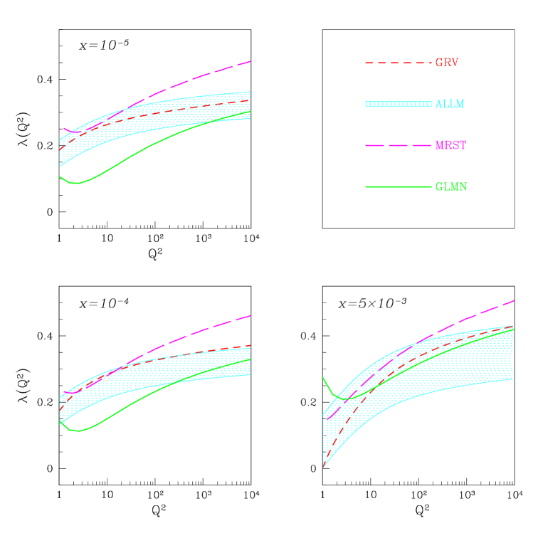
Figure 8: Comparison of different approaches: $\lambda(Q^{2})$ versus $Q^{2}$ at fixed $x$ .

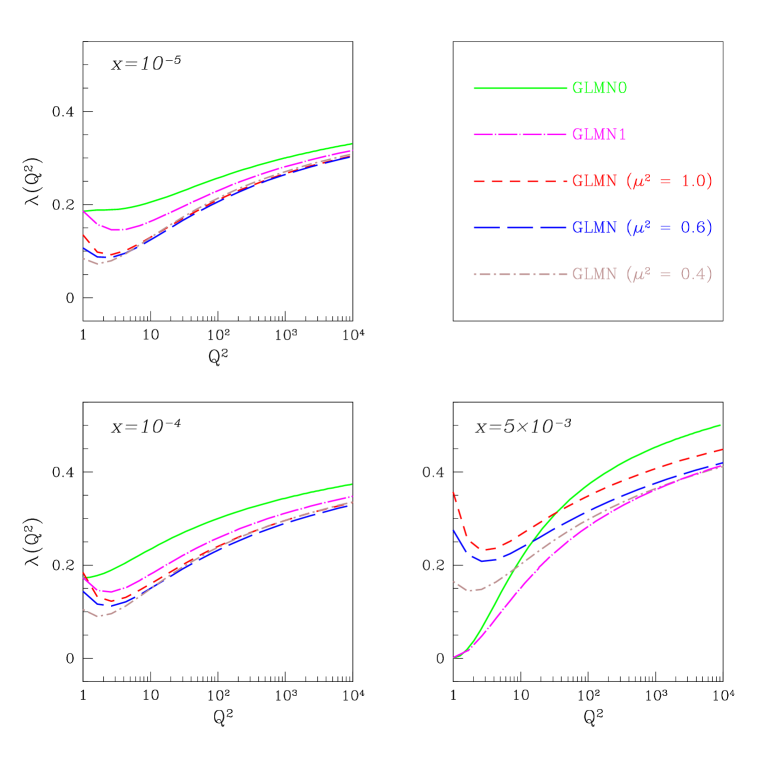
Figure 9: Comparison of different models for the long distance behaviour of $xG(x,Q^{2})$: $\lambda(Q^{2})$ versus $Q^{2}$ at fixed $x$ .

5 Summary and Conclusions

In this paper we have attempted a detailed and systematic study of the proton structure function logarithmic derivatives $\frac{\partial F_{2}(x,Q^{2})}{\partial\ln Q^{2}}$ and $\frac{\partial\ln F_{2}(x,Q^{2})}{\partial\ln(1/x)}$. Our calculations are carried out in the double log approximation of pQCD, including SC of the calculated quantities. The SC are calculated in the Eikonal model. Our study was motivated by the recent HERA results on $\frac{\partial F_{2}(x,Q^{2})}{\partial\ln Q^{2}}$ showing a considerable departure from the DGLAP predictions in the kinematical domain of small $Q^{2}<5{\,\mbox{GeV}^{2}}$ and $x<10^{-3}$.

A unique feature of our approach is that we compare our results with a pseudo data base, which is computer generated from the ALLM’97 parameterization. This is done so as to overcome the lack of detailed experimental data at sufficiently small $x$ and $Q^{2}$. This enables us to examine the fine details of our theoretical predictions, a task which can not be accomplished with the limited relevant experimental data presently available.

The main conclusions of our study are:

1. Our approach, in which we correct the unscreened DGLAP predictions for the effects of screening, enables us to achieve results on both logarithmic slopes of $F_{2}$, which are in good agreement with, both the real and pseudo data, at $x<10^{-1}$.

2. The main feature of our investigation of $\frac{\partial F_{2}(x,Q^{2})}{\partial\ln Q^{2}}$ is shown in Fig.5 . It may appear that the particular structure of $\frac{\partial F_{2}(x,Q^{2})}{\partial\ln Q^{2}}$, evident in the ZEUS data, indicates that once $x$ is small enough then $\frac{\partial F_{2}(x,Q^{2})}{\partial\ln Q^{2}}$ changes from an increasing to a decreasing function of $\frac{1}{x}$. This is not the structure suggested by our calculations. We demonstrated that $\frac{\partial F_{2}(x,Q^{2})}{\partial\ln Q^{2}}$ at fixed $Q^{2}$ both in our calculations, and in the pseudo data, remains a monotonic increasing function of $\frac{1}{x}$, in a good agreement with asymptotic expectations. The SC only suppress the rate of such growth in comparison with the DGLAP approach. It is the combination of different $\left(x,Q^{2}\right)$ data points which creates the particular structure seen in ZEUS data, and reproduced in our calculation.

3. At low $Q^{2}$ we expect $\frac{\partial F_{2}(x,Q^{2})}{\partial\ln Q^{2}}$ to be proportional to $Q^{2}$, and therefore to decrease as $Q^{2}\rightarrow 0$. This result is in full agreement with our calculations, as is evident from Fig.7 . Comparison with the MRST parameterization shows that this effect can be reproduced in the evolution equation, by suppressing the value of gluon (quark) structure function at low $x$ in initial partons distributions.

4. Since the damping of $\frac{\partial F_{2}(x,Q^{2})}{\partial\ln Q^{2}}$ is significant only for small $Q^{2}<5{\,\mbox{GeV}^{2}}$ and $x<10^{-3}$, our calculations are on the boundary of being able to use pQCD. Moreover, this is a kinematic domain where both “soft” and “hard” dynamics are significant. Our calculations suggest a smooth transition between the “soft” and the “hard” domains, and as a consequence of this, the results that we obtain from “hard” pQCD calculations are shown to be stable, and compatible with the real and pseudo data. This observation is of a particular significance for the calculations of SC in the gluon sector, where our calculation also receives contributions from relatively long distances, for which pQCD provides no estimation of errors. We suggest that a scale of hardness be defined from the solution of Eq. (23). The above gives hope that the transition from ”hard” to ”soft” mechanism can be calculated theoretically. We consider this paper, together with our earlier Ref.[10], as a first attempt to quantify this description.

5. Our study of $\lambda\left(Q^{2}\right)=\frac{\partial\ln F_{2}(x,Q^{2})}{\partial\ln(1/x)}$ is compatible with both the real and pseudo data. We confirm the expected asymptotic behaviour of $\lambda$ in the region of very small $x$ (see Fig.9). However, we would like to point out, that from Fig.8 one can see that the pseudo data indicate a different $x$ dependence of $\lambda(Q^{2})$ than our calculations. Only real data at low $x$ can clarify the situation.

6. Our general approach was to start from the unscreened DGLAP, for which we assess GRV’94 to be most suitable, and then correct for the effects of screening. An alternative approach would be evolving parton distributions, as done in [5]. There are however, two main differences between our approach and MRST: the first is a practical deficiency of MRST, which is applicable only for $Q^{2}>1.25{\,\mbox{GeV}^{2}}$ – this limit is somewhat high for the present analysis. The second is the different predictions between our approach and the MRST parameterization, in the region of small $x\sim 10^{-5}$ (see Figs.6 – 9).

We firmly believe that the experimental systematic studies of the $F_{2}$ slopes as well as other observables that are sensitive to the value of SC ( $F_{2}(charm)$, $F_{L}$ , $\frac{\partial F^{DD}_{2}(x,Q^{2})}{\partial\ln Q^{2}}$  etc. ), are needed to check one of the most fundamental problem of QCD: the value of the scale of the transition between perturbative and non-perturbative QCD.

Acknowledgments: We thank H. Abramowitz and A. Levy for providing us with a detailed program and for discussions on the ALLM’97 parameterization. This research was supported it part by the Israel Science Foundation, founded by the Israel Academy of Science and Humanities.

References

-
[1]
ZEUS Collaboration; J. Breitweg et al.: Phys. Lett. B407 (1997) 432; M. Derrick et
al.: Z. Phys. C69 (1996) 607, Z. Phys. C72 (1996) 394;
H1 Collaboration; S.Aid et al.: Nucl. Phys. B470 (1996) 3, Nucl. Phys. B497 (1997) 3. - [2] A. Caldwell: Invited talk in the DESY Theory Workshop, DESY, Octorber 1997.
- [3] V.N. Gribov and L.N. Lipatov: Sov. J. Nucl. Phys.15(1972)438; L.N. Lipatov: Yad. Fiz.20 (1974) 181; G. Altarelli and G. Parisi: Nucl. Phys. B126 (1977) 298; Yu.L.Dokshitzer: Sov.Phys. JETP 46 (1977) 641.
- [4] M. Gluck, E. Reya and A. Vogt: Z. Phys. C67 (1995) 433.
- [5] A.D. Martin, R.G. Roberts, W.J. Stirling and R.S. Thorne: “Parton distributions: a new global analysis”, DTP/98/10; hep-ph/9803445.
- [6] H. Abramowicz, E. Levin, A. Levy and U. Maor: Phys. Lett. B269 (1991) 465.
- [7] A.D. Martin, R.G. Roberts and W.J. Stirling: Phys. Lett. B387 (1996) 419.
- [8] CTEQ-collaboration: H.-L. Lai et al.: Phys. Rev. D55 (1997) 1280; J.Huston et.al.: hep-ph/9801444.
- [9] L. V. Gribov, E. M. Levin and M. G. Ryskin: Phys.Rep. 100 (1983) 1.
- [10] E. Gotsman,E. Levin and U. Maor: Phys. Lett. B425 (1998) 369.
- [11] J. Bartels, K. Charchula and F. Feltesse: Proceedings of the Workshop “ Physics at HERA” Oct.29 -30,1991, ed. W. Buchmueller and G. Ingelman, v.1, p.193.
- [12] H. Abramowicz and A. Levy: “The ALLM parameterization of an upgrade”, DESY 97-251, hep-ph/9712415.
- [13] D,O, Caldwell et al.: Phys. Rev. Lett. 40 (1978) 1222; S.I. Alekhin et al.: CERN–HERA 87–01 (1987); BCDMS Collaboration, A.C. Benvenuti et al.: Phys. Lett. B223 (1989) 485; L.W. Whitlow: SLAC–357 (1990); ZEUS Collaboration, M. Derrick et al.: Z. Phys. C63 (1994) 391; H1 Collaboration, S. Aid et al.: Z. Phys. C69 (1995) 27; E665 Collaboration, M.R. Adams et al.: Phys. Rev. D54 (1996) 3006; NMC Collaboration, M. Arneodo et al.: Nucl. Phys. B483 (1997) 3.
- [14] E.M. Levin and M.G.Ryskin: Sov. J. Nucl. Phys. 45 (1987) 150.
- [15] A.H. Mueller: Nucl. Phys. B335 (1990) 115.
- [16] B.Z. Kopeliovich et.al.: Phys. Lett. B324 (1994) 469; S.J. Brodsky et.al.: Phys. Rev. D50 (1994) 3134; L.Frankfurt, G.A. Miller and M. Strikman: Phys. Rev. D304 (1993) 1; E. Gotsman, E.M. Levin and U. Maor: Phys. Lett. B353 (1995) 526; L. Frankfurt, W. Koepf and M.Strikman: Phys. Rev. D54 (1996) 3194; A.L.Ayala Filho, M.B. Gay Ducati and E.M. Levin: Nucl. Phys. B493(1997) 305; B510 (1998) 355; E. Gotsman, E. Levin and U. Maor: Nucl. Phys. B493 (1997) 354.
- [17] E. Gotsman, E.M. Levin and U. Maor: DESY 97-154, TAUP 2443-97, hep-ph/ 9708275, EPJ (in press).
- [18] J.C. Collins, D.E. Soper and G. Sterman: Nucl. Phys.B308 (1988) 833.
- [19] A.L.Ayala Filho, M.B. Gay Ducati and E.M. Levin: Phys. Lett. B388 (1996) 189.
- [20] E. Gotsman, E. Levin and U. Maor: Phys. Lett. B403 (1997) 120.
- [21] E. Gotsman, E. Levin and U. Maor: Phys. Lett. B353 (1995) 526.
- [22] A.L.Ayala Filho, M.B. Gay Ducati and E.M. Levin: Nucl. Phys. B493(1997) 305.
- [23] E. Gotsman, E.M. Levin and U. Maor: Nucl. Phys. B493 (1997) 354.
- [24] M. Abramowitz and I.A,Stegun: “Handbook of Mathematical Functions”, Dover, New York, 1970.
- [25] A.H. Mueller: “Small and diffraction scattering”, plenary talk at DIS’98, Brussels, April 4-8,1998.