OUTP-98-60-P
Instantons and the QCD Vacuum Wavefunctional

Abstract

We analyze the instanton transitions in the framework of the gauge invariant variational calculation in the pure Yang-Mills theory. Instantons are identified with the saddle points in the integration over the gauge group which projects the Gaussian wave functional onto the gauge invariant physical Hilbert space. We show that the dynamical mass present in the best variational state provides an infrared cutoff for the instanton sizes. The instantons of the size $\rho<1/M$ are suppressed and the large size instanton problem arising in the standard WKB calculation is completely avoided in the present variational framework.

I Introduction

In recent years there have been renewed interest in application of the Hamiltonian methods to the study of nonabelian Yang-Mills theories [1, 2, 3, 4, 5]. One set of these works [1, 3, 4] attempts to solve “exactly” the strongly interacting gauge theories in the sense that a nonlinear transformation is performed to a set of gauge invariant coordinates. One then tries to find a controlled expansion akin to strong coupling perturbation theory, which hopefully solves the infrared part of the theory in the leading order. Another set [2, 5] attempts to find the Yang-Mills vacuum wave functional with the help of a variational approximation. In particular in [2] a gauge invariant generalization of a Gaussian variational approximation was developed. The hope of this approach is that the vacuum of QCD may be not very different from the vacuum of a free theory in many important respects. This hope rests on the observation that many genuine nonperturbative effects in QCD appear already on the momentum scales much larger than $\Lambda_{\rm QCD}$ where the coupling constant is still small [6]. It may be possible then to account for these effects with the Gaussian wave functional, which is similar to the ground state of the free theory modifying only the width of the Gaussian for the low momentum modes. This modification is essentially nonperturbative and should lead to the generation of the same condensates that account for a variety of QCD phenomenology via the QCD sum rules [6].

The variational calculations of [2] are of exploratory nature and many questions regarding their validity remain unsettled. Some of those are discussed in the original paper [2] as well as in [10]. Nevertheless this variational approach captures many of the essential features of gluodynamics; mass generation, formation of the gluon condensate, [2], and asymptotic freedom, [7, 8, 10]. Possible appearance of the linear potential between static quarks in this approach has also been discussed [9, 10, 11]. In fact one of the nicer features of this approximation is that it exhibits nontrivial nonperturbative infrared physics (gluon condensate) along with correct weak coupling ultraviolet behavior (one loop Yang-Mills $\beta$ function). If so one is naturally lead to ask whether it also gives a good account of the instanton physics. Instantons are the only concrete description of the non-perturbative nature of the QCD vacuum in the path integral formalism. In the ultraviolet region although the effect of the instantons is nonperturbatively small they are easily identifiable. They should therefore serve as a useful probe for any non-perturbative approach especially if it purports to capture both the infrared and the ultraviolet physics. The aim of the present paper is precisely to study the structure and the properties of the instantons in the variational approach of [2].

Instantons are localized, finite-action classical solutions of the field equations of QCD in Euclidean space-time [12]. Such solutions have been obtained in exact analytical form, and extensively studied. An excellent review of instantons in gauge theories can be found in [13] and [14].

Physically instantons represent tunneling processes between topologically distinctive vacuum sectors with the exponent of the instanton action being equal to the transition probability between two of these vacuum states. As any tunneling probability at weak coupling it is nonperturbatively small (of order $\exp(-{const}/\alpha_{S})$) and the instantons therefore are invisible in the weak coupling perturbation theory. When first discovered there was hope that instantons would provide the solution to the strong coupling problem[15, 16]. Although it has been subsequently realized that instantons are irrelevant for understanding confinement, they have provided a beautiful mechanism of spontaneous chiral symmetry breaking [17]. The instanton liquid model (initially introduced on phenomenological grounds [18], and later justified by Euclidean variational methods [19]) to this day remains the most complete theory of chiral symmetry breaking in QCD. It is therefore vital to understand the properties of the instantons if one is hoping to extend the application of the Gaussian variational approximation to QCD with fermions.

Although the notion of the instanton is intrinsically Euclidean, the tunneling between different vacuum sectors can be formulated in the Hamiltonian language as well as in the Lagrangian one. In fact the gauge projected formalism of [2] is very well suited for this purpose. The projection of the initial Gaussian onto the gauge invariant subspace is achieved by the integration over the gauge group. As will be explained in detail later, the $SU(N)$ matrix $U(x_{i})$ (the dependence here is on the spatial coordinates only) in this type of calculation turns out to play the role of a $\sigma$-model field. This field is governed by an “action”, whose structure depends on the parameters of the variational state. As we shall see, the Yang-Mills instantons correspond to the topologically nontrivial saddle points of this action. In this paper we will study the properties of these saddle point solutions.

Our main result is the following. We find that the appearance of the dynamical mass parameter in the variational state stabilizes the size of the instantons. Recall, that the main unsolved problem of the dilute instanton gas approximation is that (when account is taken of the one loop running of the coupling constant) the path integral is dominated by the large size instantons. The measure for the integration over the sizes diverges as a power in the infrared and this divergence renders the dilute gas calculation meaningless. It is usually assumed that this infrared divergence is eliminated by some nonperturbative effects. This is precisely what we find in the variational approach. The dynamical mass $M$ present in the best variational state suppresses instantons of sizes $\rho>1/M$. The size of the stable instanton that we find turns out to be consistent with the average size of the instanton in the instanton liquid model.

This paper is structured as follows. In section II we briefly recall the formalism and the results of [2]. We explain how to identify the tunneling transition in this framework and what type of classical configuration should be identified with the instanton. It is also noted that the generation of the dynamical mass itself found in [2] can be directly interpreted in terms of the condensation of these instantons.

In section III we study numerically the structure and the action of the small size instantons. For these instantons the presence of the dynamical mass is irrelevant and this calculation is performed at zero mass. The profile function of the instanton and the value of the transition probability are approximately determined by a variational method. We find that the tunneling probability indeed scales as $\exp\{-c\alpha_{s}\}$ with the value of $c$ approximately two times larger than in the standard Euclidean calculation. We explain why this discrepancy is not unexpected in a variational calculation.

In section IV corrections to the solution and the action due to a non-zero mass gap are calculated. It is found that the instanton is stabilized to a size of the order of the inverse mass scale. This size is directly comparable with that found in the instanton liquid model.

Finally, sectionV is devoted to discussion of our results and their relation with the instanton liquid model.

II The Hamiltonian portrait of an instanton

We start with a brief description of the gauge invariant Gaussian approximation of [2]. The Ansatz for the QCD wavefunctional considered in [2] is,

$$\Psi[A_{i}^{a}]=\int DU(x_{i})\Psi_{U}[A],$$ (1)

with,

$$\Psi_{U}[A]=\exp\left\{-{1\over 2}\int d^{3}xd^{3}y\ A_{i}^{Ua}(x)G_{ij}^{-1ab}(x-y)\ A_{j}^{Ub}(y)\right\}.$$ (2)

Here $A^{U}$ is the gauge transform of the vector potential with the gauge transformation $U$.

$$A_{i}^{Ua}(x)=S^{ab}(x)A_{i}^{b}(x)+\lambda_{i}^{a}(x),$$ (3)

with,

$$S^{ab}(x) = \frac{1}{2}{\rm tr}\left[\tau^{a}U^{\dagger}(x)\tau^{b}U(x)\right],$$ (4)

$$\lambda_{i}^{a}(x) = \frac{i}{g}{\rm tr}\left[\tau^{a}U^{\dagger}(x)\partial_{i}U(x)\right].$$ (5)

The SU(N) generators are taken to satisfy the following algebra and normalization,

$$[\tau^{a},\tau^{b}]=2if^{abc}\tau^{c},\;\;\;\frac{1}{2}{\rm tr}[\tau^{a}\tau^{b}]=\delta^{ab}.$$ (6)

The state thus constructed obeys Gauss’ law since it is explicitly invariant under the gauge transformation $A_{i}(x)\rightarrow A_{i}^{V}(x)$ with arbitrary $SU(N)$ matrix $V(x)$. The width of the Gaussian $G(x)$ is a parameter with respect to which the expectation value of the Hamiltonian is varied. A simple rotation and (global) color invariant form is $G_{ij}^{-1ab}=\delta_{ij}\delta^{ab}G^{-1}$. The functional form of $G^{-1}$ is chosen to agree with the perturbation theory in the limit of high momentum on one hand, and to allow for the nonperturbative mass scale on the other,

$$G^{-1}(k)=\left\{\begin{array}[]{ll}\sqrt{k^{2}~{}}&\mbox{ if $k^{2}>M^{2}$}\\ M&\mbox{ if $k^{2}<M^{2}$}\end{array}\right..$$ (9)

Technically, the calculation of the expectation values of gluonic operators in the state eq.(1) is mapped into the calculation in a nonlocal nonlinear $\sigma$-model in three Euclidean dimensions. Consider the vacuum average of an arbitrary gauge invariant operator $O[A]$,

$$\langle O\rangle = \frac{1}{Z}\int DA\Psi^{*}[A]O[A]\Psi[A]={1\over Z}\int DU_{1}DU_{2}DA\Psi_{U_{1}}^{*}[A]O[A]\Psi_{U_{2}}[A]$$ (10)

$$= {1\over Z}\int DUDA\Psi_{1}^{*}[A]O[A]\Psi_{U}[A].$$ (11)

In the last line the matrix $U=U^{\dagger}_{1}U_{2}$ is the relative gauge transformation between the two Gaussian wave functions. The normalization factor $Z$ (the norm of the state) is,

$$Z=\int DUDA\Psi_{1}^{*}[A]\Psi_{U}[A].$$ (12)

The Gaussian integration over the gauge potential $A_{i}$ can be performed explicitly. As a result the last step of the calculation is a path integral over the $SU(N)$ matrix $U$ with the $\sigma$-model partition function,

$$Z=\int DU\exp\{-\Gamma[U]\},$$ (13)

where the (nonlocal) action is,

$$\Gamma[U]=\frac{1}{2}\lambda\Delta\lambda+\frac{1}{2}{\rm Tr}{\rm ln}{\cal M}.$$ (14)

Here summation over all indices (rotational, color and coordinate) is implied. The first term is written explicitly as,

$$\frac{1}{2}\int d^{3}x\ d^{3}y\ \lambda_{i}^{a}(x)\Delta^{ac}(x,y)\lambda_{i}^{c}(y),$$ (15)

with,

$$\Delta^{ac}(x,y)=[\delta^{ac}G(x-y)+S^{ab}(x)G(x-y)S^{cb}(y)]^{-1}.$$ (16)

In eq.(14) we have defined,

$\displaystyle{\cal M}^{ab}_{ij}(x,y)=\left[S^{Tac(x)}S^{cb}(y)+\delta^{ab}\right]\,G^{-1}(x-y)\,\delta_{ij}.$

The second term in eq.(14) is of $O(g^{2})$ relative to the first one and with the accuracy of [2] can be ignored. We will not consider it in the following. The action of the $\sigma$-model eq.(15) depends on the variational parameter $M$ through eq.(16). The minimization of the expectation value of the energy in [2] leads to a nonzero value of the mass parameter $M$ in the best variational state. The dynamical mass parameter is determined by the relation

$$\alpha_{s}(M_{0})={\pi\over 4N_{c}},$$ (17)

where the Yang-Mills coupling constant $\alpha_{s}$ evolves according to one loop $\beta$-function. The significance of this value of $M$ from the point of view of the effective $\sigma$ model is that at this point it undergoes the phase transition. For $M<M_{0}$ the model is in the weakly coupled ordered phase. In this phase the matrix $U$ is close to the unit matrix with small fluctuations around it. For $M>M_{0}$ the model is in the disordered phase. The matrix $U$ fluctuates strongly so that it covers all available phase space and its average value vanishes. It was found in [2] that the energy is minimized just above the phase transition $M=M_{0}+$ so that the $\sigma$-model is in the disordered phase.

Coming back to the subject of the present paper, the first thing is to understand how do we expect to see instantons in this formalism. The answer to this is the following. As explained above the effective $\sigma$-model arises as an integration over the relative gauge transformations between the two Gaussian states in the linear superposition eq.(1). The Boltzmann factor $\exp(-\Gamma[U])$ for a given matrix $U$ is therefore just the overlap of the initial and the gauge rotated state, or in other words the transition amplitude between the two states. The instanton transition is precisely the transition of this type, where the two states are related by a large gauge transformation. The matrix of this large gauge transformation must carry a nonzero topological charge $\Pi_{3}(SU(N))$.

The integration measure over $U$ indeed includes integration over topologically nontrivial configurations. The finiteness of the action eq.(15) requires that the matrix $U$ approaches constant value at infinity. This identifies all points at spatial infinity hence, the physical space of the model is $S^{3}$. Field configurations are maps from $S^{3}$ into the manifold of $SU(N)$ and are classified by their winding number, or topological charge, which is an element of the homotopy group $\Pi_{3}(SU(N))=Z$. The $\sigma$-model action in a given topological sector is minimized on some configuration which is a solution of classical $\sigma$-model equations of motion. In particular, the solution with a unit topological charge is expected to have a “hedgehog” structure much like the topological soliton in the Skyrme model[20]. The integral over $U$ in the steepest descent approximation is saturated by these classical solutions.

These $\sigma$-model configurations that belong to a nontrivial topological sector with a unit winding number represent QCD transitions between the topologically distinct sectors. The topologically nontrivial classical soliton solutions of the $\sigma$-model are therefore the three dimensional images of the QCD instantons.

The QCD instantons are defined in space time and are therefore four dimensional point-like objects. The $\sigma$-model solutions are intrinsically three dimensional. Nevertheless, there is a natural simple relation between the two. For a given Yang-Mills instanton solution $A^{\rm inst}(x_{\mu})$ one can find a three dimensional $SU(N)$ matrix $U(x_{i})$ by the procedure discussed by Atiyah and Manton, [21],

$$U_{\rm AM}(x_{i})=P\exp\left(i\int_{C}dx^{\mu}A^{\rm inst}_{\mu}\right),$$ (18)

where the contour of integration $C$ is a straight line $x_{i}=const$, $-\infty<x_{0}<\infty$. The matrix $U_{\rm AM}$ gives the relative gauge transformation between the initial trivial vacuum at $x_{0}\rightarrow-\infty$ and the topologically nontrivial vacuum at $x_{0}\rightarrow+\infty$, or in other words between the initial and final states of the instanton transition. Clearly, its meaning is precisely the same as of the classical soliton solution of the effective $\sigma$-model eq.(15). Also, the QCD instanton action and the $\sigma$-model soliton action have the same physical meaning. They both give the transition probability between different topological sectors in QCD. We will therefore refer to the $\sigma$-model solitons as instantons in the following.

One has to realize that although the QCD and the $\sigma$ - model instantons have the same physical meaning, it is not assured that the numerical value for their respective actions is the same. They both approximate the value of the transition probability in QCD, but the approximations involved are quite different. The QCD instanton action is the result of the standard WKB approximation which is valid at weak coupling and therefore for small instantons, but breaks down for instantons of large size. The $\sigma$ - model instanton action on the other hand is the value of this transition probability in a particular Gaussian variational approximation. It is natural to expect that variational calculation underestimates the value of the transition probability at very weak coupling. The transition probability is given by the overlap of the “ground state” wave functions in two topological sectors. For simplicity let us consider a quantum mechanical system with two vacua at $x_{\pm}$. If the area below the barrier separating the vacua is large, the standard WKB instanton calculation is applicable. The wave function of each of the vacua below the barrier has essentially an exponential fall off $\exp\{i\int^{x}\sqrt{E-V(x-x_{\pm})}\}$. The instanton calculation is the calculation of the overlap of these functions. Our variational calculation corresponds to approximating the respective “ground states” at $x_{\pm}$ by Gaussian wave functions. The tails of the Gaussians fall off much faster away from the minimum than the actual wave function and the overlap is therefore is expected to be smaller. When the coupling constant is not too small (or when the area below the barrier is not too large) the overlap between the two states is not determined any more by the behavior of the “tails” of the wave functions. In this situation one can expect the Gaussian approximation to do much better, since the overlap region contributes significantly to the energy and therefore plays important role in the minimization procedure.

The rest of this paper is devoted to a quantitative study of instantons in the variational state eq.(1). Before proceeding to this part, however, we would like to note that implicitly the instantons played a very important role already in the energy minimization of [2]. As we mentioned above the energy is minimized for the value of the mass parameter $M$ at which the $\sigma$ model is in the disordered phase. The transition between ordered and disordered phases in a statistical mechanical system can usually be described as a condensation of topological defects. This is a standard description of the phase transition in the Ising and XY models [22]. In the $\sigma$ model eq.(15) the relevant topological defects are none other than the instantons. In this sense the appearance of the dynamical mass in the best variational state itself is driven by the condensation of instantons.

III Small Size Instantons

In this section we wish to study small size instantons. For the instanton solutions of a size $\rho<<1/M$ the presence of a finite dynamical mass is irrelevant. We will therefore take $M=0$ for the calculations in this section. The existence of a finite mass scale is very important for the instantons of large size and will be taken into account in the next section. It somewhat increases the complexity of the calculation but all the necessary methods can be developed for the $M=0$ case.

For $M=0$ the inverse propagator (9) which defines the variational state eqs.(1,2) is (in momentum space) $G^{-1}(k)=|k|$. We find it more convenient to work in coordinate space throughout the rest of this paper. Fourier transforming $G^{-1}$ to the coordinate space according to the definition,

$$G^{-1}(k)=(2\pi)^{-3/2}\int d^{3}xG^{-1}(x)e^{ikx},$$ (19)

we find,

$$G^{-1}(x-y)=-\frac{1}{\pi^{2}}\left(\frac{\Theta(|x-y|-\Lambda^{-1})}{|x-y|^{4}}-\Lambda^{3}\delta(|x-y|-\Lambda^{-1})\right).$$ (20)

Here we had to introduce the ultraviolet cutoff $\Lambda$ to define the coordinate space expression properly. The coefficient of the second term is determined by requiring that at finite cutoff $\Lambda$,

$$\int dx^{3}G^{-1}(x)\propto G^{-1}(k=0)=0.$$ (21)

Note that $\Lambda$ is introduced as a regulator only and no subtraction in the expression for the propagator (or the action) was performed. The cutoff $\Lambda$ should be taken to infinity at the end of the calculation and the results of the calculation should be finite in this limit. Below we show how the divergent terms cancel exactly, so that in the numerical calculations we only take into account finite terms in the limit $\Lambda\to\infty$.

We are searching for an instanton solution of topological charge one to the action (15). Such a solution should have the maximally symmetric “hedgehog” form,

$$U(x)=e^{i\tau^{a}\hat{x}^{a}f(r)}=\cos{f(r)}+i\tau^{a}\hat{x}^{a}\sin{f(r)},$$ (22)

where $\tau^{a}$ are the generators of $SU(2)$ and $f(r)$ is an unspecified function of $r=|x|$, which we will refer to as the profile function. The profile function is constrained to satisfy $f(0)=\pi$ and $f(\infty)=0$, which ensures that the field configuration eq.(22) has unit topological charge. We need only consider the group $SU(2)$ since the solutions for $SU(N>2)$ can be found from the embedding of $SU(2)$ in $SU(N)$, [23]. Substituting this form for the field into the components of the action, we find,

$$\lambda_{i}^{a}(x) = \frac{i}{g}{\rm tr}[\tau^{a}U^{+}(x)\partial_{i}U(x)]$$ (23)

$$= -\frac{2}{g}\hat{x}^{i}\hat{x}^{a}f^{\prime}(r)-\frac{1}{gr}(\delta^{ia}-\hat{x}^{i}\hat{x}^{a})\sin{2f(r)}-\frac{2}{g}\epsilon_{abi}\frac{\hat{x}^{b}}{r}\sin^{2}f(r),$$ (24)

$$S^{ab}(x) = \frac{1}{2}{\rm tr}[\tau^{a}U^{+}(x)\tau^{b}U(x)]$$ (25)

$$= \delta^{ab}-\epsilon_{abc}\hat{x}^{c}\sin{2f(r)}+2(\hat{x}^{a}\hat{x}^{b}-\delta^{ab})\sin^{2}f(r),$$ (26)

where $\epsilon_{abc}$ is the antisymmetric tensor. For the hedgehog configuration, the function $S^{ab}(x)$ differs significantly from $\delta^{ab}$ only over a small region, the size of which depends on how fast the transition is from the asymptotic behavior at large distance to that at small distance. If the profile function has a sharp transition between these two limits one can reasonably approximate $S^{ab}$ by $\delta^{ab}$. Once the form of the profile function has been found this can be checked for consistency. It is possible to expand around $S^{ab}=\delta^{ab}$ and systematically calculate corrections in $S^{ab}-\delta^{ab}$. At the end of this section we calculate the leading correction and find that it is indeed small for the instanton profile function.

This approximation allows us to write,

$$\Delta^{ac}(x,y)=[\delta^{ac}G(x-y)+S^{ab}(x)G(x-y)S^{cb}(y)]^{-1}\simeq\frac{1}{2}G^{-1}(x-y)\delta^{ac}.$$ (27)

With the definition eq.(20), we write the action eq.(15) as,

$$\Gamma = \Gamma_{1}-\Gamma_{2},$$ (28)

$$\Gamma_{1} = -\frac{1}{4\pi^{2}}\int d^{3}xd^{3}y\lambda_{i}^{a}(x)\frac{\Theta(|x-y|-\Lambda^{-1})}{|x-y|^{4}}\lambda_{i}^{a}(y),$$ (29)

$$\Gamma_{2} = -\frac{\Lambda^{3}}{4\pi^{2}}\int d^{3}xd^{3}y\lambda_{i}^{a}(x)\delta(|x-y|-\Lambda^{-1})\lambda_{i}^{a}(y).$$ (30)

Both $\Gamma_{1}$ and $\Gamma_{2}$ are divergent. The divergences between the two terms however cancel leaving the action finite. Changing variables, $u_{i}=x_{i}+y_{i}$, $v_{i}=x_{i}-y_{i}$, and using the fact that $2|v|^{-4}=\nabla^{2}_{v}|v|^{-2}$, we find after integrating by parts twice,

$$\Gamma_{1} = -\frac{1}{64\pi^{2}}\int d^{3}ud^{3}v|v|^{-2}\nabla^{2}_{v}\left[\lambda_{i}^{a}(x)\lambda_{i}^{a}(y)\right]+\Gamma_{\rm surf}+\Gamma_{\rm div},$$ (31)

$$\Gamma_{\rm surf} = \left.-\frac{1}{64\pi^{2}}\int d^{3}ud\Omega_{v}\left(2|v|^{-1}+\partial_{|v|}\right)\left[\lambda_{i}^{a}(x)\lambda_{i}^{a}(y)\right]\right|_{|v|=\infty},$$ (32)

$$\Gamma_{\rm div} = \left.\frac{1}{64\pi^{2}}\int d^{3}ud\Omega_{v}\left(2|v|^{-1}+\partial_{|v|}\right)\left[\lambda_{i}^{a}(x)\lambda_{i}^{a}(y)\right]\right|_{|v|=\Lambda^{-1}},$$ (33)

where $d\Omega_{v}$ denotes angular integration in $v$-space, and $\nabla^{2}_{v}$ is the $v$-space Laplacian. The divergent part $\Gamma_{\rm div}$ cancels exactly the “subtraction” term $\Gamma_{2}$ when $\Lambda\rightarrow\infty$. Moreover, the surface terms $\Gamma_{\rm surf}$ vanish if the profile $f(r)$ approaches zero as $r^{-2}$ or faster at infinity, and is infinite otherwise. In what follows we assume that $f(r)$ decreases fast enough. Ignoring all terms in the action which vanish in the limit $\Lambda\to\infty$ we are left with the finite, cutoff independent action,

$$\Gamma=-\frac{1}{8\pi^{2}}\int d^{3}xd^{3}y\frac{1}{|x-y|^{2}}\left(\frac{\partial^{2}}{\partial x_{j}^{2}}+\frac{\partial^{2}}{\partial y_{j}^{2}}-2\frac{\partial^{2}}{\partial x_{j}\partial y_{j}}\right)\left[\lambda_{i}^{a}(x)\lambda_{i}^{a}(y)\right].$$ (34)

For the hedgehog configuration (22),

$$\lambda_{i}^{a}(x)\lambda_{i}^{a}(y) = \frac{1}{g^{2}}\left[4\cos^{2}\theta f^{\prime}(r)f^{\prime}(s)+\frac{2}{s}(1-\cos^{2}\theta)f^{\prime}(r)\sin{2f(s)}\right.$$ (37)

$$+\frac{2}{r}(1-\cos^{2}\theta)f^{\prime}(s)\sin{2f(r)}+\frac{1}{rs}(1+\cos^{2}\theta)\sin{2f(r)}\sin{2f(s)}$$

$$+\left.\frac{8}{rs}\cos\theta\sin^{2}f(r)\sin^{2}f(s)\right],$$

where $\cos\theta=\hat{x}\cdot\hat{y}$, $r=|x|$ and $s=|y|$. From (37) we see that $\lambda_{i}^{a}(x)\lambda_{i}^{a}(y)$ is a function of only three variables, $\lambda_{i}^{a}(x)\lambda_{i}^{a}(y)=\frac{1}{g^{2}}\sum_{n=0}^{2}\cos^{n}\theta\,H_{n}(r,s)$, where $H_{n}$ are immediately found from (37). They are given explicitly in the Appendix for easy reference. We also give in the Appendix the coefficient functions $\tilde{H}_{n}(r,s)$ which are defined by,

$$\left(\frac{\partial^{2}}{\partial x_{j}^{2}}+\frac{\partial^{2}}{\partial y_{j}^{2}}-2\frac{\partial^{2}}{\partial x_{j}\partial y_{j}}\right)\left[\lambda_{i}^{a}(x)\lambda_{i}^{a}(y)\right]=\frac{1}{g^{2}}\sum_{n=0}^{3}\cos^{n}\theta\,\tilde{H}_{n}(r,s).$$ (38)

After carrying out the angular integrations we get an action as a functional of the profile function,

$$\Gamma=-\frac{2}{g^{2}}\int dr\,ds\,(rs)^{2}\sum_{n=0}^{3}I_{n}(r,s)\tilde{H}_{n}(r,s),$$ (39)

where,

$$I_{n}(r,s)=\int_{-1}^{1}\frac{d(\cos{\theta})\cos^{n}\theta}{(r^{2}+s^{2}-2rs\cos\theta)},$$ (40)

are given in the Appendix.

We were unable to minimize the action with respect to the profile function by analytical methods. We have therefore employed a variational method to determine the best profile function approximately. The two important variational parameters are the ones that govern the asymptotic behavior of $f(r)$,

$$\left\{\begin{array}[]{lcl}f\sim r^{-\alpha}&&r\rightarrow\infty\\ f\sim\pi-r^{\beta}&&r\rightarrow 0\\ \end{array}\right..$$ (41)

The dependence on the parameter $\alpha$ which determines the asymptotics at large distance turns out to be simple. Using two trial functions,

$$f_{1}(r) = \pi\left[\frac{\rho^{\alpha}}{\rho^{\alpha}+x^{\alpha}}\right],$$ (42)

$$f_{2}(r) = 2\arctan{(\rho/r)^{\alpha}},$$ (43)

and performing the double numerical integration we have found that the action monotonically increases with $\alpha$. This means that the optimal value for this parameter is $\alpha=2$, since this is the lowest possible value at which the surface terms are non-infinite.

Having fixed $\alpha$, we next studied the dependence on the parameter $\beta$ which determines the behavior close to the instanton center. The trial functions we used for this purpose are,

$$f_{1}(r) = \pi\left[\frac{\rho^{\beta}}{\rho^{\beta}+x^{\beta}}\right]^{2/\beta},$$ (44)

$$f_{2}(r) = 2\arctan\left(\frac{2}{(r/\rho)^{2}+(r/\rho)^{\beta}}\right).$$ (45)

We find numerically the optimal value for the parameter $\beta$ to be $\beta=1.1$ for $f_{1}$ and $\beta=1.0$ for $f_{2}$.

The corresponding values for the action are

$$\Gamma=1.75\frac{8\pi^{2}}{g^{2}},$$ (46)

for $f_{1}$, and

$$\Gamma=1.73\frac{8\pi^{2}}{g^{2}},$$ (47)

for $f_{2}$.

We have calculated the first correction $\Delta\Gamma$ to the action in the expansion of $S^{ab}$ around $\delta_{ab}$ for the two profiles. We find $\Delta\Gamma=0.21\frac{8\pi^{2}}{g^{2}}$ for $f_{1}$ and $\Delta\Gamma=0.34\frac{8\pi^{2}}{g^{2}}$ for $f_{2}$. The correction to the action for both profiles is of order of $10\%$. Note however, that the Ansatz $f_{1}$ is more stable, and indeed after the correction is taken into account has lower action than $f_{2}$.

The corrected (to this order) values for the action are

$$\Gamma=1.96\frac{8\pi^{2}}{g^{2}},$$ (48)

for $f_{1}$, and

$$\Gamma=2.07\frac{8\pi^{2}}{g^{2}},$$ (49)

for $f_{2}$.

Note that although our Ansatze for the profile function depend on the instanton size $\rho$, the value of the action does not depend on it. This is the direct consequence of the dilatational invariance of the effective $\sigma$-model action eq.(27). The introduction of the cutoff $\Lambda$ strictly speaking breaks the dilatational invariance. This breaking however is very small and the invariance is restored in the limit $\Lambda\rightarrow\infty$.

We now want to comment on the numerical value of the transition probability obtained in our variational approach. Our result eq.(48) should be compared with the value $8\pi^{2}/g^{2}$ for the classical action of a Yang-Mills instanton. So the action of an instanton in the variational approach is about two times larger than the standard path integral result and the transition probability therefore appears to be much smaller. As explained in Section II it is in fact natural to expect this sort of behavior in the Gaussian approximation since the tails of the Gaussians fall off much faster away from the minimum than the actual wave function and the overlap is therefore smaller. This is the basic reason for the discrepancy in the numerical values of the action between the variational instanton of this section and the weak coupling (WKB) instanton of the standard path integral approach.

It is significant that both the asymptotic behavior and the value of the action for both our variational Ansatze for the profile function is very similar to the corresponding results for the Atiyah-Manton Ansatz[21]. As discussed in Section II, the natural identification between the QCD instanton and the instanton in the effective $\sigma$-model is furnished by the holonomy along all time-lines,

$$U(x)={\rm T}\exp\left[-\int_{-\infty}^{\infty}dx^{\mu}A_{\mu}^{\rm inst}(x)\right].$$ (50)

For the QCD instanton eq.(50) results in the profile function,

$$f_{\rm AM}(r)=\pi\left[1-\left(1+\frac{\rho^{2}}{r^{2}}\right)^{-\frac{1}{2}}\right].$$ (51)

The asymptotics of this configuration at large distances is $f(r)\propto 1/r^{2}$, and near the instanton core $f(r)-\pi\propto r$. This gives $\alpha=2$, $\beta=1$ for the Atiyah-Manton configuration, identical with $f_{2}$ and practically indistinguishable from $f_{1}$. In fact the profile $f_{\rm AM}$ is very similar to $f_{1}$ not only asymptotically but also in the whole range $0<r<\infty$. In Fig. 1 we plot the three profile functions for the same value of the instanton size. It is clear that $f_{1}$ and $f_{\rm AM}$ are very similar while $f_{2}$ differs from them somewhat inside the instanton core. We also note that $f_{2}$ has a slower approach to its value at $r=0$, which explains why the value of the action for this profile is less stable against the $S^{ab}-\delta^{ab}$ corrections.

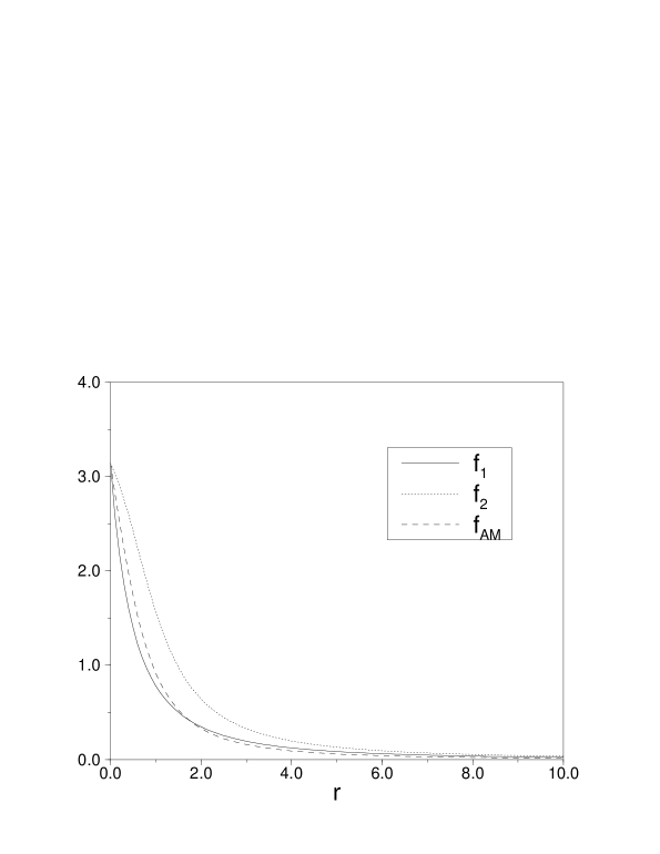
FIG. 1.: The hedgehog profile functions $f_{1}$, $f_{2}$ and $f_{\rm AM}$ for $\rho=1$.

We have calculated the $\sigma$-model action for the Atiyah-Manton profile numerically and found (including the first correction in $S^{ab}-\delta^{ab}$ expansion) $\Gamma=1.97\frac{8\pi^{2}}{g^{2}}$. This again is very close to the value we obtain with our variational Ansatz eq.(48). This means that even though the value of the transition probability is underestimated in the Gaussian approximation, the actual field configurations into which the tunneling is most probable are identified correctly–they are precisely the same as in the WKB calculation.

It should be noted that the exact value of the transition probability due to small size instantons (very weak coupling) is not so important, since they do not significantly affect the structure of the vacuum in any case. It would therefore be incorrect to declare the Gaussian approximation as a failure from the instanton point of view. One expects the Gaussian approximation to do much better at intermediate couplings, since the overlap region contributes significantly to the energy and therefore plays important role in the minimization procedure. In the Yang-Mills framework this means that there are two types of instantons configurations that we expect to contribute significantly and therefore to be better described by the Gaussian approximation. First, these are large instantons for which the coupling constant is not small and the action not large. Those are presicely the configurations that cause problems in dilute instanton gas approximation. The second class is the multi-instanton configurations, where the separation between instantons is not too large and the interaction between them is not negligible. These are the configurations of the instanton liquid type. As discussed in the previous section, these configurations are in fact responsible for the generation of the dynamical scale in the best variational state through the condensation of instantons. The direct discussion of these multi-instanton configuration is however beyond the scope in the present paper. The large size instantons, or rather the instantons of the size comparable to the dynamical scale $1/M$ are the subject of the next section.

IV Mass Correction and Instantons of Stable Size

We now want to explore the effect of the dynamical mass on the properties of the instantons. Our expectation is that the presence of the mass scale stabilizes the size of the instantons and suppresses the instantons of the sizes larger than $1/M$.

The simple qualitative argument to this effect is the following. Consider the effective $\sigma$-model action for very large size instantons. In such a configuration only field modes with small momentum $k<M$ are present. For these momenta the action simplifies, and as discussed in [2] the action eq.(15) becomes the standard local $\sigma$-model where $M$ plays the role of the ultraviolet cutoff.

$$\Gamma={1\over 2}{M\over g^{2}(M)}tr\int d^{3}x~{}\partial_{i}U^{\dagger}(x)\partial_{i}U(x)$$ (52)

If the large size instantons are stable at all they should also be present as stable solutions in this local action eq.(52). However this is not the case as can be easily seen by the standard Derrick type scaling argument. Take an arbitrary configuration $u(x)$ in the instanton sector and scale all the coordinates by a common factor $\lambda$. Then obviously

$$\Gamma[u(\lambda x)]=\lambda^{-1}\Gamma[u(x)]$$ (53)

The dependence of the action on $\lambda$ is monotonic and is minimized at $\lambda\rightarrow\infty$. This means that the instantons in the local $\sigma$-model shrink to the ultraviolet cutoff $1/M$. For instantons smaller than the inverse cutoff we can not use the local action anymore. However the behavior of these small size instantons is already familiar. We know that when the running of the coupling is taken into account, these instantons are pushed to the large size. This is the infrared problem of large instantons we alluded to earlier. In our variational state the coupling constant stops running at the scale $M$. The picture is therefore very simple. The small size instantons are pushed to larger size by the effect of the coupling constant, while the large size instantons are pushed to smaller size by the effect of the local $\sigma$-model scaling. It is therefore clear that the size will be stabilized somewhere in the vicinity of $\rho\sim 1/M$.

To confirm this picture we now turn to the numerical evaluation of the instanton action. We write the inverse propagator (9) as,

$$G^{-1}(k)=G_{0}^{-1}(k)+\Delta G^{-1}(k),$$ (54)

where

$$G_{0}^{-1}(k) = |k|$$ (55)

$$\Delta G^{-1}(k) = \theta(M-|k|)\ (M-|k|)$$ (56)

Since the action eq.(15) is linear in $G^{-1}$, the $G_{0}^{-1}$ term will lead to the classical action $\Gamma_{0}$ calculated in the previous section. As discussed above, $\Gamma_{0}$ is scale invariant and therefore does not depend on the size of the instanton. In coordinate space, the second term in eq.(54) reads,

$$\Delta G^{-1}(|x-y|)=-\frac{1}{\pi^{2}|x-y|^{4}}\left(\cos{M|x-y|}-1+\frac{M|x-y|}{2}\sin{M|x-y|}\right).$$ (57)

The mass correction term in the propagator gives rise to the correction in the action

$$\Delta\Gamma=\frac{1}{4}\int d^{3}xd^{3}y\lambda_{i}^{a}(x)\Delta G^{-1}(x-y)\lambda_{i}^{a}(y).$$ (58)

We now compute the dependence of $\Delta\Gamma$ on the size of the instanton for the three profile functions considered above, $f_{1}$, $f_{2}$ and $f_{\rm AM}$. As before, the angular integrations can be performed exactly. We obtain,

$$\Delta\Gamma=-\frac{2}{g^{2}}\int drds(rs)^{2}\sum_{n=0}^{3}\tilde{I}_{n}(r,s)H_{n}(r,s),$$ (59)

where $H_{n}$ are as before and $\tilde{I}_{n}$ defined by

$$\tilde{I}_{n}=\int_{-1}^{1}\frac{d(\cos{\theta})\cos^{n}\theta}{(r^{2}+s^{2}-2rs\cos\theta)^{2}}\left(\cos{M|x-y|}-1+\frac{M|x-y|}{2}\sin{M|x-y|}\right),$$ (60)

are given in the Appendix.

We calculated numerically the dependence of the classical action on the size of the instanton for the three profiles (44), (45) and (51). We find that the action increases monotonically with the instanton size. The dependence of the classical action on the size for the three anzatse is shown in Fig. 2. As discussed in the beginning of this section the classical action favors small size instantons in all three Ansatze.

FIG. 2.: Dependence of the classical action on the size of the instanton for the profiles $f_{1}$, $f_{2}$ and $f_{\rm AM}$. The action is given in units of $8\pi^{2}/g^{2}$.

We now must include the effect of the running coupling constant. This is equivalent to calculating the one loop correction around the instanton background. Rather than performing this technically nontrivial calculation we will use the results of [7]. We will limit ourselves to the $SU(2)$ theory in the following. The $\beta$-function in the nonlinear $\sigma$-model was found in [7] as

$$\beta(g)=-\frac{g^{3}}{(4\pi)^{2}}8.$$ (61)

This is slightly different from the complete one loop Yang-Mills $\beta$-function. The origin of this discrepancy was studied in [7, 8] and is well understood now. It is due to the fact that the present variational calculation omits the screening contributions of the transverse gluons. As discussed in [10] the variational state can be modified to yield an exact $\beta$-function. This point is not essential for our analysis and we will not dwell on it any further except noting that the use of either eq.(61) or the exact one loop expression in the following leads to the same results.

Eq.(61) is valid at distances smaller than $1/M$. The coupling constant at these distances therefore scales according to

$$\frac{8\pi^{2}}{g^{2}(\mu>M)}=8\ln\left(\frac{\mu}{\Lambda_{\rm QCD}}\right),$$ (62)

At distances larger than $M$ the running of the coupling constant stops and it tends to a constant value,

$$\frac{8\pi^{2}}{g^{2}(\mu<M)}=8\ln\left(\frac{aM}{\Lambda_{\rm QCD}}\right).$$ (63)

with $a$, a numerical constant of order one. The precise interpolation between the two regime is unimportant and we will use the following simple interpolating expression

$$\frac{8\pi^{2}}{g^{2}(\mu)}=4\ln\left(\frac{M^{2}}{\Lambda_{\rm QCD}^{2}}\left(\frac{\mu^{2}}{M^{2}}+a\right)\right).$$ (64)

Since the exact value of the constant $a$ is not known we will present our results for several values of order one. When evaluating the action of the instanton of the size $\rho$ we obviously must take $\mu=1/\rho$.

The running of the coupling constant is not the only logarithmic effect at one loop order. In addition one has to take into account the path integral measure over the three translational zero modes and the size of the instanton,

$$dx_{1}dx_{2}dx_{3}d\rho\rho^{-4},$$ (65)

which contributes an extra term to the action,

$$\Gamma_{\rm measure}=4\log{\rho}.$$ (66)

Collecting all the one-loop logarithmic contributions together we calculate the corrected action as a function of the size of the instanton as

$$\Gamma(g^{2}(1/\rho))+\Gamma_{\rm measure}.$$ (67)

The result for the three different profiles we have considered are shown in Figs. 3, 4 and 5, for different values of the parameter $a$.

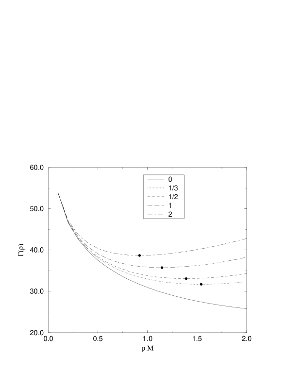
FIG. 3.: The classical action plus one-loop logarithmic corrections for the profile $f_{1}$ as a function of the instanton size. The different curves correspond to different values of the parameter $a=0,\ldots,2$, and the bullets mark the minimum of each curve.

FIG. 4.: The classical action plus one-loop logarithmic correction for the profile $f_{2}$ as a function of the instanton size. The different curves correspond to different values of the parameter $a=0,\ldots,2$, and the bullets mark the minimum of each curve.

FIG. 5.: The classical action plus one-loop logarithmic correction for the profile $f_{\rm AM}$ as a function of the instanton size. The different curves correspond to different values of the parameter $a=0,\ldots,2$, and the bullets mark the minimum of each curve.

In all cases the action has a minimum at a size of the order of $1/M$. The values for the size of the instanton, its action and the curvature at the minimum are given in Table I for different values of $a$. The results for the Atiyah-Manton Ansatz and our function $f_{1}$ are practically indistinguishable. Varying the parameter $a$ between $1/2$ and $2$ the size of the stable instanton varies between $1.5/M$ and $1/M$. The Ansatz $f_{2}$ leads to the instanton size smaller by a factor of $1.5-2$. We consider however the former estimate to be better, since the Ansatz $f_{2}$ gives a considerably larger value of the action (see Fig. 2) and is therefore not a very good choice for the instanton “valley” configuration.

	$f_{1}$			$f_{2}$			$f_{\rm AM}$
$a$	$\rho_{\rm min}$	$\Gamma(\rho_{\rm min})$	$\Gamma^{\prime\prime}(\rho_{\rm min})$	$\rho_{\rm min}$	$\Gamma(\rho_{\rm min})$	$\Gamma^{\prime\prime}(\rho_{\rm min})$	$\rho_{\rm min}$	$\Gamma(\rho_{\rm min})$	$\Gamma^{\prime\prime}(\rho_{\rm min})$
1/3	$1.5$	$32.$	$6.9$	$0.9$	$36.$	$23.$	$1.6$	$32.$	$6.3$
1/2	$1.4$	$33.$	$7.9$	$0.8$	$37.$	$26.$	$1.5$	$33.$	$7.0$
1	$1.1$	$36.$	$9.7$	$0.7$	$39.$	$33.$	$1.2$	$36.$	$8.1$
2	$0.9$	$39.$	$12.0$	$0.6$	$41.$	$41.$	$1.0$	$39.$	$9.7$

TABLE I.: Stable size $\rho_{\rm min}$ for the soliton in units of $1/M=0.75GeV^{-1}$, the value of the minimum action $\Gamma(\rho_{\rm min})$ and the curvature at the minimum $\Gamma^{\prime\prime}(\rho_{\rm min})$, for the three profiles, for different values of the parameter $a$.

The numerical analysis of this section confirms therefore our expectations. The presence of the dynamical mass stabilizes the size of the instantons at the value $\rho=\frac{1-1.5}{M}$. The large instanton problem therefore finds a nonperturbative solution in the framework of the Gaussian variational approximation.

V Discussion

In this paper we have discussed how the instanton transitions appear in the framework of the gauge invariant Gaussian approximation of [2]. The relative gauge rotation between two gauge field configurations between which the tunneling transition is most probable is determined from the saddle point equation of the effective nonlinear $\sigma$-model. We found that the relative gauge transformations for most probable tunneling transitions are very similar to the ones found in the standard path integral instanton approach.

The value of the logarithm of the tunneling probability for small size instantons however turns out to be larger by about a factor of two in the variational vacuum. This is understandable since the tail of a Gaussian wave function decreases faster and therefore the overlap integral of two such wave functions is smaller than of the semi-classical wave functions.

Our main result concerns the effect of the dynamical mass scale that characterizes the variational vacuum. We find that the presence of this scale stabilizes the size of the instanton. The instantons of the size larger than the inverse of this scale are suppressed. When account is taken of the proper running of the strong coupling constant, the integral over the instanton sizes has a saddle point. This saddle point determines the most likely size of the instanton as $\rho=1-1.5/M$. The large size instanton infrared problem which plagues the standard dilute instanton gas approximation is thereby removed in the variational vacuum due to the presence of the dynamical nonperturbative scale.

An interesting point is that the instanton action for the most likely size instanton is pretty large, the numerical value being around 35 (see Table I). This means that the configurations with small number of instantons and anti-instantons are not important energetically. Nevertheless, the generation of the dynamical mass itself within the framework of our variational approximation is due to the instanton condensation. This is so since the effective $\sigma$-model is in the disordered phase at the value of the best variational parameter $M$. This suggests that the important type of configurations are the ones that contain many instantons and anti-instantons. The small fugacity factor in these configurations can be overcome by a large entropy and also by the interaction between instantons and anti-instantons. This interaction is known to be attractive for some relative color orientation. The interaction also is quite long range, since the instanton profile function away from the instanton center decreases only as the second power of the distance. It is therefore entirely possible that the important configurations for the energy minimization are of the type of the instanton liquid–namely those having large number of instantons which although fairly dilute nevertheless feel each others presence strongly due to the long range interaction. It is in fact interesting to note that the most likely instanton size we found here is consistent with the average size of the instantons in the instanton liquid model of [18, 19]. For the case of $SU(2)$, the average instanton size, in units of the gluon condensate obtained in the instanton liquid model, turns out to be [19],

$\displaystyle\rho\,\left(\langle F_{\mu\nu}^{a}F_{\mu\nu}^{a}\rangle\alpha/\pi\right)^{1/4}\sim.4.$

In our case, taking the value of the gluon condensate obtained in the variational approach [2], we find,

$\displaystyle\rho\,\left(\langle F_{\mu\nu}^{a}F_{\mu\nu}^{a}\rangle\alpha/\pi\right)^{1/4}\sim.2-.3.$

The relation of the variational approach with the instanton liquid model is a very interesting open question and warrants further study.

The finite action for the case of the mass scale $M=0$ is given in (34). To obtain the explicit action for the profile of the hedgehog field (22) it is necessary to calculate the Laplacian over $v=x-y$ of the product of the right currents $\lambda^{a}_{i}$ at the points $x$ and $y$, which has the form

$$\lambda_{i}^{a}(x)\lambda_{i}^{a}(y)=\frac{1}{g^{2}}\sum_{n=0}^{2}\cos^{n}\theta H_{n}(r,s).$$ (68)

The expression for $H_{n}$ are obtained from (37),

$$H_{0} = \frac{1}{rs}\sin{2f(r)}\sin{2f(s)}+\frac{2}{r}\sin{2f(r)}f^{\prime}(s)+\frac{2}{s}\sin{2f(s)}f^{\prime}(r),$$ (69)

$$H_{1} = \frac{8}{rs}\sin^{2}f(r)\sin^{2}f(s),$$ (70)

$$H_{2} = \frac{1}{rs}\left(\sin{2f(r)}-2rf^{\prime}(r)\right)\left(\sin{2f(s)}-2sf^{\prime}(s)\right).$$ (71)

After calculating the Laplacian over $v$ we obtain

$$\left(\frac{\partial^{2}}{\partial x_{j}^{2}}+\frac{\partial^{2}}{\partial y_{j}^{2}}-2\frac{\partial^{2}}{\partial x_{j}\partial y_{j}}\right)\left[\lambda_{i}^{a}(x)\lambda_{i}^{a}(y)\right]=\frac{1}{g^{2}}\sum_{n=0}^{3}\cos^{n}\theta\tilde{H}_{n}(r,s).$$ (72)

From Eq. (37) the expressions for $\tilde{H}_{n}(r,s)$ can be found:

$$2r^{3}s^{3}\tilde{H}_{0}(r,s)=8\,r\,s\,\sin^{2}f(r)\,\sin^{2}f(s)+{r^{2}}\,\sin{2\,f(r)}\,\sin{2\,f(s)}$$ (78)

$$-16\,{r^{2}}\,s\,\cos{f(r)}\,\sin{f(r)}\,\sin^{2}f(s)\,f^{\prime}(r)-2\,{r^{3}}\,\sin{2\,f(s)}\,f^{\prime}(r)$$

$$-2\,{r^{2}}\,{s^{2}}\,\sin{2\,f(r)}\,\sin{2\,f(s)}\,{{f^{\prime}(r)}^{2}}-2\,{r^{2}}\,s\,\sin{2\,f(r)}\,f^{\prime}(s)$$

$$+4\,{r^{3}}\,s\,f^{\prime}(r)\,f^{\prime}(s)-4\,{r^{3}}\,{s^{2}}\,\sin{2\,f(s)}\,f^{\prime}(r)\,{{f^{\prime}(s)}^{2}}+2\,{r^{2}}\,{s^{2}}\,\sin{2\,f(s)}\,f^{\prime\prime}(r)$$

$$+{r^{2}}\,{s^{2}}\,\cos{2\,f(r)}\,\sin{2\,f(s)}\,f^{\prime\prime}(r)+2\,{r^{3}}\,{s^{2}}\,\cos{2\,f(s)}\,f^{\prime}(r)\,f^{\prime\prime}(s)$$

$$+{r^{3}}\,{s^{2}}\,\sin{2\,f(s)}\,f^{(3)}(r)+(r\leftrightarrow s),$$

$$2r^{3}s^{3}\tilde{H}_{1}(r,s)=-8\,{r^{2}}\,\sin^{2}f(r)\,\sin^{2}f(s)+3\,r\,s\,\sin{2\,f(r)}\,\sin{2\,f(s)}$$ (84)

$$-4\,{r^{2}}\,s\,\sin{2\,f(s)}\,f^{\prime}(r)-2\,{r^{2}}\,s\,\cos{2\,f(r)}\,\sin{2\,f(s)}\,f^{\prime}(r)$$

$$+8\,{r^{2}}\,{s^{2}}\,{{\cos{f(r)}}^{2}}\,\sin^{2}f(s)\,{{f^{\prime}(r)}^{2}}+8\,{r^{2}}\,{s^{2}}\,\cos{2\,f(r)}\,f^{\prime}(r)\,f^{\prime}(s)$$

$$-4\,{r^{2}}\,{s^{2}}\,\cos{2\,f(r)}\,\cos{2\,f(s)}\,f^{\prime}(r)\,f^{\prime}(s)-8\,{r^{2}}\,{s^{2}}\,\sin^{2}f(r)\,\sin^{2}f(s)\,{{f^{\prime}(s)}^{2}}$$

$$+8\,{r^{2}}\,{s^{2}}\,\cos{f(r)}\,\sin{f(r)}\,\sin^{2}f(s)\,f^{\prime\prime}(r)+6\,{r^{3}}\,s\,\sin{2\,f(s)}\,f^{\prime\prime}(r)$$

$$-8\,{r^{3}}\,{s^{2}}\,f^{\prime}(s)\,f^{\prime\prime}(r)-4\,{r^{3}}\,{s^{2}}\,\cos{2\,f(s)}\,f^{\prime}(s)\,f^{\prime\prime}(r)+(r\leftrightarrow s),$$

$$2r^{3}s^{3}\tilde{H}_{2}(r,s)=-32\,r\,s\,\sin^{2}f(r)\,\sin^{2}f(s)-3\,{r^{2}}\,\sin{2\,f(r)}\,\sin{2\,f(s)}$$ (92)

$$+32\,{r^{2}}\,s\,\cos{f(r)}\,\sin{f(r)}\,\sin^{2}f(s)\,f^{\prime}(r)+6\,{r^{3}}\,\sin{2\,f(s)}\,f^{\prime}(r)$$

$$-2\,{r^{2}}\,{s^{2}}\,\sin{2\,f(r)}\,\sin{2\,f(s)}\,{{f^{\prime}(r)}^{2}}+6\,{r^{2}}\,s\,\sin{2\,f(r)}\,f^{\prime}(s)$$

$$-12\,{r^{3}}\,s\,f^{\prime}(r)\,f^{\prime}(s)-32\,{r^{2}}\,{s^{2}}\,\cos{f(r)}\,\cos{f(s)}\,\sin{f(r)}\,\sin{f(s)}\,f^{\prime}(r)\,f^{\prime}(s)$$

$$+4\,{r^{2}}\,{s^{3}}\,\sin{2\,f(r)}\,{{f^{\prime}(r)}^{2}}\,f^{\prime}(s)-2\,{r^{2}}\,{s^{2}}\,\sin{2\,f(s)}\,f^{\prime\prime}(r)$$

$$+{r^{2}}\,{s^{2}}\,\cos{2\,f(r)}\,\sin{2\,f(s)}\,f^{\prime\prime}(r)+4\,{r^{2}}\,{s^{3}}\,f^{\prime}(s)\,f^{\prime\prime}(r)$$

$$-2\,{r^{3}}\,{s^{2}}\,\cos{2\,f(s)}\,f^{\prime}(r)\,f^{\prime\prime}(s)-{r^{3}}\,{s^{2}}\,\sin{2\,f(s)}\,f^{(3)}(r)$$

$$+2\,{r^{3}}\,{s^{3}}\,f^{\prime}(s)\,f^{(3)}(r)+(r\leftrightarrow s),$$

$$2r^{3}s^{3}\tilde{H}_{3}(r,s)=-9\,r\,s\,\sin{2\,f(r)}\,\sin{2\,f(s)}+12\,{r^{2}}\,s\,\sin{2\,f(s)}\,f^{\prime}(r)$$ (97)

$$+6\,{r^{2}}\,s\,\cos{2\,f(r)}\,\sin{2\,f(s)}\,f^{\prime}(r)-16\,{r^{2}}\,{s^{2}}\,f^{\prime}(r)\,f^{\prime}(s)$$

$$-8\,{r^{2}}\,{s^{2}}\,\cos{2\,f(r)}\,f^{\prime}(r)\,f^{\prime}(s)-4\,{r^{2}}\,{s^{2}}\,\cos{2\,f(r)}\,\cos{2\,f(s)}\,f^{\prime}(r)\,f^{\prime}(s)$$

$$-6\,{r^{3}}\,s\,\sin{2\,f(s)}\,f^{\prime\prime}(r)+8\,{r^{3}}\,{s^{2}}\,f^{\prime}(s)\,f^{\prime\prime}(r)+4\,{r^{3}}\,{s^{2}}\,\cos{2\,f(s)}\,f^{\prime}(s)\,f^{\prime\prime}(r)$$

$$-4\,{r^{3}}\,{s^{3}}\,f^{\prime\prime}(r)\,f^{\prime\prime}(s)+(r\leftrightarrow s).$$

The expressions for the angular integrals (40) appearing in the action (39) are the following:

$$I_{0} = \frac{1}{2rs}\log\left[\frac{(r+s)^{2}}{(r-s)^{2}}\right],$$ (98)

$$I_{1} = -\frac{1}{rs}+\frac{(r^{2}+s^{2})}{4r^{2}s^{2}}\log\left[\frac{(r+s)^{2}}{(r-s)^{2}}\right],$$ (99)

$$I_{2} = -\frac{1}{2r^{2}}-\frac{1}{2s^{2}}+\frac{(r^{2}+s^{2})^{2}}{8r^{3}s^{3}}\log\left[\frac{(r+s)^{2}}{(r-s)^{2}}\right],$$ (100)

$$I_{3} = -\frac{1}{3rs}-\frac{(r^{2}+s^{2})^{2}}{4r^{3}s^{3}}+\frac{(r^{2}+s^{2})^{3}}{16r^{4}s^{4}}\log\left[\frac{(r+s)^{2}}{(r-s)^{2}}\right].$$ (101)

The corresponding integrals (60) for the case of $M\neq 0$ read:

$$\tilde{I}_{0} = \frac{1}{rs}\left(\frac{\sin^{2}(t/2)}{t^{2}}\right)_{M|r-s|}^{M(r+s)},$$ (102)

$$\tilde{I}_{1} = \frac{r^{2}+s^{2}}{2rs}\tilde{I}_{0}+\frac{1}{2r^{2}s^{2}}\left(\frac{\cos{t}}{2}-{\rm ci}(t)+\ln(t/2)\right)_{M|r-s|}^{M(r+s)},$$ (103)

$$\tilde{I}_{2} = \frac{r^{2}+s^{2}}{2rs}\tilde{I}_{1}-\frac{1}{8r^{3}s^{3}}\left[(-4+t^{2}-r^{2}-s^{2})\cos{t}\right.$$ (105)

$$+\left.2(r^{2}+s^{2})({\rm ci}(t)-\ln{(t/2)})+t(t-4\sin{t})\right]_{M|r-s|}^{M(r+s)},$$

where ${\rm ci}(t)$ is the Cosine-integral function

$${\rm ci}(t)=-\int_{t}^{\infty}\frac{\cos{t}}{t}dt.$$ (106)

REFERENCES

- [1] M. Bauer, D.Z. Freedman and P.E. Haagensen, Nucl. Phys. B428, 147 (1994), hep-th/9505028; M. Bauer, D.Z. Freedman, Nucl. Phys. B450, 209 (1995); hep-th/9505144;
- [2] I. Kogan and A. Kovner, Phys.Rev. D 52 (1995) 3719.
- [3] P. Mansfield, Phys.Lett. B358, 287 (1995), hep-th/9508148; Phys.Lett. B365, 207 (1996), hep-th/95010188; P. Mansfield and M. Sampaio, hep-th/9807163.
- [4] D. Karabali and V. P. Nair, Nucl.Phys. B464, 135 (1996), hep-th/9510157; D. Karabali, C. Kim and V. P. Nair, Nucl.Phys. B524, 661 (1998), hep-th/9705087; D. Karabali, C. Kim and V. P. Nair, hep-th/9804132.
- [5] C. Heineman, C. Martin, D. Vautherin, E. Iancu, hep-th/9802036.
- [6] M. Shifman, A. Vainshtein and V. Zakharov, Nucl. Phys. B147, 385 (1979).
- [7] W.E. Brown and I. Kogan, to appear in Int. J. Mod. Phys. A, hep-th/9705136.
- [8] W. E. Brown, to appear in Int. J. Mod. Phys. A, hep-th/9711189.
- [9] K. Zarembo, Phys. Lett. 421B, 325 (1998), hep-th/9710235.
- [10] D. I. Diakonov, “Trying to Understand Confinement in the Schrodinger Picture”, 1998, lectures given at the 4th St. Petersburg Winter School in Theoretical Physics, hep-th/9805137.
- [11] A. Kovner and B. Svetitsky, to appear.
- [12] A.A. Belavin, A.M. Polyakov, A.S. Schwartz and Yu. S. Tyupkin, Phys. Lett. 59B, 85 (1975).
- [13] M.A. Shifman, Instantons in Gauge Theories (World Scientific, Singapore, 1994).
- [14] R. Rajaraman, Solitons and Instantons (North-Holland, Amsterdam, 1987).
- [15] C. Callan, R. Dashen and D. Gross, Phys. Rev. D 17, 10 (1978).
- [16] C. Callan, R. Dashen and D. Gross, Phys. Rev. D 19, 1826 (1979).
- [17] D. Dyakonov, “Chiral Symmetry Breaking by Instantons”, lectures at the Enrico Fermi School in Physics, 1995, hep-ph/9602375.
- [18] E. Shuryak, Nucl. Phys. B203, 93 (1982); B203, 117 (1982).
- [19] D. Dyakonov and V. Petrov, Nucl. Phys. B245, 259 (1984); E. Shuryak, Nucl. Phys. B328, 102 (1989); E. Shuryak and J. Verbaaschot, Nucl. Phys. B341, 1 (1990).
- [20] Selected Papers, with Commentary, of Tony Royle Hilton Skyrme, ed. G. Brown (World Scientific, Singapore, 1994).
- [21] M. Atiyah and N. Manton, Phys. Lett. 222B, 438 (1989).
- [22] J. Kogut, Rev. Mod. Phys. 51, 659 (1979).
- [23] C. Bernard, Phys. Rev. D 19, 3013 (1979); F. Wilczek, Phys. Lett. 65B, 160 (1976).