FACTORIZATION AND EFFECTIVE ACTION FOR HIGH-ENERGY SCATTERING IN QCD

Abstract

I demonstrate that the amplitude of the high-energy scattering can be factorized in a convolution of the contributions due to fast and slow fields. The fast and slow fields interact by means of Wilson-line operators – infinite gauge factors ordered along the straight line. The resulting factorization formula gives a starting point for a new approach to the effective action for high-energy scattering.

Talk given at “Continious Advances in QCD”, Minnesota, April 16-19, 1998

1 Introduction

The starting point of almost every perturbative QCD calculation is a factorization formula of some sort. A classical example is the factorization of the structure functions of deep inelastic scattering into coefficient functions and parton densities. The form of factorization is dictated by process kinematics (for a review, see[1]). In case of deep inelastic scattering, there are two different scales of transverse momentum and it is therefore natural to factorize the amplitude in the product of contributions of hard and soft parts coming from the regions of small and large transverse momenta, respectively. On the contrary, in the case of high-energy (Regge-type) processes, all the transverse momenta are of the same order of magnitude, but colliding particles strongly differ in rapidity. Consequently, it is natural to look for factorization in the rapidity space.

The basic result of the paper is that the high-energy scattering amplitude can be factorized in a convolution of contributions due to “fast” and “slow” fields. To be precise, we choose a certain rapidity $\eta_{0}$ to be a “rapidity divide” and we call fields with $\eta>\eta_{0}$ fast and fields with $\eta<\eta_{0}$ slow where $\eta_{0}$ lies in the region between spectator rapidity and target rapidity. (The interpretation of this fields as fast and slow is literally true only in the rest frame of the target but we will use this terminology for any frame).

Our starting point is the operator expansion for high-energy scattering [2] where the explicit integration over fast fields gives the coefficient functions for the Wilson-line operators representing the integrals over slow fields. For a 2$\Rightarrow$2 particle scattering in Regge limit $s\gg m^{2}$ (where $m$ is a common mass scale for all other momenta in the problem $t\sim p_{A}^{2}\sim(p^{\prime}_{A})^{2}\sim p_{B}^{2}\sim(p^{\prime}_{B})^{2}\sim m^{2}$) we have:

$$A(p_{A},p_{B}\Rightarrow p^{\prime}_{A},p^{\prime}_{B})=$$

$$\sum\int d^{2}x_{1}...d^{2}x_{n}C^{i_{1}...i_{n}}(x_{1},...x_{n})\langle p_{B}|{\rm Tr}\{U_{i_{1}}(x_{1})...U_{i_{n}}(x_{n})\}|p^{\prime}_{B}\rangle$$

(As usual, $s=(p_{A}+p_{B})^{2}$ and $t=(p_{A}-p^{\prime}_{A})^{2}$). Here $x_{i}~{}(i=1,2)$ are the transverse coordinates (orthogonal to both $p_{A}$ and $p_{B}$) and $U_{i}(x)=U^{\dagger}(x){i\over g}{\partial\over\partial x_{i}}U(x)$ where the Wilson-line operator $U(x)$ is the gauge link ordered along the infinite straight line corresponding to the “rapidity divide” $\eta_{0}$. Both coefficient functions and matrix elements in Eq. (1) depend on the $\eta_{0}$ but this dependence is canceled in the physical amplitude just as the scale $\mu$ (separating coefficient functions and matrix elements) disappears from the final results for structure functions in case of usual factorization. Typically, we have the factors $\sim(g^{2}\ln s/m^{2}-\eta_{0})$ coming from the “fast” integral and the factors $\sim g^{2}\eta_{0}$ coming from the “slow” integral so they combine in a usual log factor $g^{2}\ln s/m^{2}$. In the leading log approximation these factors sum up into the BFKL pomeron[3],[4] (for a review see ref. [5]). Note, however, that unlike usual factorization, the expansion (1) does not have the additional meaning of perturbative $vs$ nonperturbative separation – both the coefficient functions and the matrix elements have perturbative and non-perturbative parts. This happens due to the fact that the coupling constant in a scattering processis is determined by the scale of transverse momenta. When we perform the usual factorization in hard ($k_{\perp}>\mu$) and soft ($k_{\perp}<\mu$) momenta, we calculate the coefficient functions perturbatively (because $\alpha_{s}(k_{\perp}>\mu)$ is small) whereas the matrix elements are non-perturbative. Conversely, when we factorize the amplitude in rapidity, both fast and slow parts have contributions coming from the regions of large and small $k_{\perp}$. In this sense, coefficient functions and matrix elements enter the expansion (1) on equal footing. We could have integrated first over slow fields (having the rapidities close to that of $p_{B}$) and the expansion would have the form:

$$A(s,t)=\sum\int d^{2}x_{1}...d^{2}x_{n}D^{i_{1}...i_{n}}(x_{1},...x_{n})\langle p_{A}|{\rm Tr}\{U_{i_{1}}(x_{1})...U_{i_{n}}(x_{n})\}|p^{\prime}_{A}\rangle$$ (2)

In this case, the coefficient functions $D$ are the results of integration over slow fields ant the matrix elements of the $U$ operators contain only the large rapidities $\eta>\eta_{0}$. The symmetry between Eqs. (1) and (2) calls for a factorization formula which would have this symmetry between slow and fast fields in explicit form.

Our goal is to demonstrate that one can combine the operator expansions (1) and (2) in the following way:

$$A(s,t)=\sum{i^{n}\over n!}\int d^{2}x_{1}...d^{2}x_{n}$$

$$\langle p_{A}|U^{a_{1}i_{1}}(x_{1})...U^{a_{n}i_{n}}(x_{n})|p^{\prime}_{A}\rangle\langle p_{B}|U^{a_{1}}_{i_{1}}(x_{1})...U^{a_{n}}_{i_{n}}(x_{n})|p^{\prime}_{B}\rangle$$

where $U^{a}_{i}\equiv{\mathop{\rm Tr}}(\lambda^{a}U_{i})$ ($\lambda^{a}$ are the Gell-Mann matrices). It is possible to rewrite this factorization formula in a more visual form if we agree that operators $U$ act only on states $B$ and $B^{\prime}$ and introduce the notation $V_{i}$ for the same operator as $U_{i}$ only acting on the $A$ and $A^{\prime}$ states:

$$A(s,t)=\langle p_{A}|\langle p_{B}|\exp\left(i\!\int\!d^{2}xV^{ai}(x)U^{a}_{i}(x)\right)|p^{\prime}_{A}\rangle|p^{\prime}_{B}\rangle$$ (4)

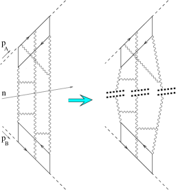
Figure 1: Structure of the factorization formula. Dashed, solid, and wavy lines denote photons, quarks, and gluons, respectively. Wilson-line operators are denoted by dotted lines and the vector $n$ gives the direction of the “rapidity divide” between fast and slow fields

In a sense, this formula amounts to writing the coefficient functions in Eq. (1) (or Eq. (2)) as matrix elements of Wilson-line operators. (Such an idea was first discussed in ref. [6]). Eq. (4) illustrated in Fig.1 is our main result and the rest of the paper is devoted to the derivation of this formula and the discussion of its possible applications.

2 Operator expansion for high-energy scattering

Let us now briefly remind how to obtain the operator expansion (1). For simplicity, consider the classical example of high-energy scattering of virtual photons with virtualities $\sim-~{}m^{2}$.

$$A(s,t)=-i{\mbox{$\langle 0|$}}T\{j(p_{A})j(p^{\prime}_{A})j(p_{B})j(p^{\prime}_{B})\}{\mbox{$|0\rangle$}}.$$ (5)

where $j(p)$ is the Fourier transform of electromagnetic current $j_{\mu}(x)$ multiplied by some suitable polarization $e^{\mu}(p)$. At high energies it is convenient to use the Sudakov decomposition:

$$p^{\mu}~{}=~{}\alpha_{p}p_{1}^{\mu}+\beta_{p}p_{2}^{\mu}+p_{\perp}^{\mu}$$ (6)

where $p_{1}^{\mu}$ and $p_{2}^{\mu}$ are the light-like vectors close to $p_{A}$ and $p_{B}$, respectively ($p_{A}^{\mu}=p_{1}^{\mu}-p_{2}^{\mu}p_{A}^{2}/s,~{}p_{B}^{\mu}=p_{2}^{\mu}-p_{1}^{\mu}p_{B}^{2}/s$). We want to integrate over the fields with $\alpha>\sigma$ where $\sigma$ is defined in such a way that the corresponding rapidity is $\eta_{0}$. (In explicit form $\eta_{0}=\ln{\sigma\over\tilde{\sigma}}$ where $\tilde{\sigma}\equiv{m^{2}\over s\sigma}$). The result of the integration will be given by Green functions of the fast particles in slow “external” fields[2] (see also ref.[7]). Since the fast particle moves along a straight-line classical trajectory, the propagator is proportional to the straight-line ordered gauge factor $U$ [8]. For example, when $x_{+}>0,~{}y_{+}<0$ it has the form[2]:

$$G(x,y)=i\int\!dz\delta(z_{\ast})\frac{(\not\!\!x-\not\!\!z)\not\!\!p_{2}}{2\pi^{2}(x-z)^{4}}U(z_{\perp})\frac{\not\!\!z-\not\!\!y}{2\pi^{2}(z-y)^{4}}$$ (7)

We use the notations $z_{\bullet}\equiv z_{\mu}p_{1}^{\mu}$ and $z_{\ast}\equiv z_{\mu}p_{2}^{\mu}$ which are essentially identical to the light-front coordinates $z_{+}=z_{*}/\sqrt{s},~{}z_{-}=z_{\bullet}/\sqrt{s}$. The Wilson-line operator $U$ is defined as

$$U(x_{\perp})=[\infty p_{1}+x_{\perp},-\infty p_{1}+x_{\perp}]$$ (8)

where $[x,y]$ is the straight-line ordered gauge link suspended between the points $x$ and $y$:

$$[x,y]{\stackrel{{\scriptstyle\rm def}}{{\equiv}}}P\exp\left(ig\int_{0}^{1}du(x-y)^{\mu}A_{\mu}(ux+(1-u)y)\right)$$ (9)

The origin of Eq. (7) is more clear in the rest frame of the “A” photon (see Fig.2).

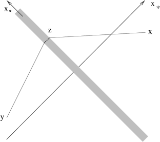
Figure 2: Quark propagator in the shock-wave background

fields are approaching this quark at high speed. Due to the Lorentz contraction, these fields are squeezed in a shock wave located at $z_{*}=0$. Therefore, the propagator (7) of the quark in this shock-wave background is a product of three factors which reflect (i) free propagation from $x$ to the shock wave (ii) instantaneous interaction with the shock wave which is described by the operator $U(z_{\perp})$, and (iii) free propagation from the point of interaction $z$ to the final destination $y$.

The propagation of the quark-antiquark pair in the shock-wave background is described by the product of two propagators of Eq. (7) type which contain two Wilson-line factors $U(z)U^{\dagger}(z^{\prime})$ where $z^{\prime}$ is the point where the antiquark crosses the shock wave. If we substitute this quark-antiquark propagator in the original expression for the amplitude (5) we obtain[2]:

$$\int\!d^{4}xd^{4}ze^{ip_{A}\cdot x+iq\cdot z}\langle T\{j(x+z)j(z)\}\rangle_{A}\simeq\int\frac{d^{2}p_{\perp}}{4\pi^{2}}I(p_{\perp},q_{\perp}){\mathop{\rm Tr}}\{U(p_{\perp})U^{\dagger}(q_{\perp}-p_{\perp})\}$$

where $U(p_{\perp})$ is the Fourier transform of $U(x_{\perp})$ and $I(p_{\perp},q_{\perp})$ is the so-called “impact factor” which is a function of $p_{\perp}^{2},p_{\perp}\!\cdot\!q_{\perp}$, and photon virtuality [9],[2]. Thus, we have reproduced the leading term in the expansion (1). (To recognize it, note that $U(x_{\perp})U^{\dagger}(y_{\perp})=P\exp\left\{-ig\int^{x}_{y}dz_{i}U_{i}(z_{\perp})\right\}$ where the precise form of the path between points $x_{\perp}$ and $y_{\perp}$ does not matter since this is actually a formula for the gauge link in a pure gauge field $U_{i}(z_{\perp})$).

Note that formally we have obtained the operators $U$ ordered along the light-like lines. Matrix elements of such operators contain divergent longitudinal integrations which reflect the fact that light-like gauge factor corresponds to a quark moving with speed of light (i.e., with infinite energy). As demonstrated in [2], we may regularize this divergence by changing the slope of the supporting line: if we wish the longitudinal integration stop at $\eta=\eta_{0}$, we should order our gauge factors $U$ along a line parallel to $n=\sigma p_{1}+\tilde{\sigma}p_{2}$. Then the coefficient functions in front of Wilson-line operators will contain logarithms $\sim g^{2}\ln 1/\sigma$. For example, there are corrections of such type to the impact factor $I(p,q)$ and if we sum them, the impact factor will be replaced by $\sum\left(g^{2}\ln 1/\sigma\right)^{n}{\cal K}^{n}I(p,q)$ where ${\cal K}$ is the BFKL kernel.

Factorization formula for high-energy scattering

In order to understand how this expansion can be generated by the factorization formula of Eq. (1) type we have to rederive the operator expansion in axial gauge $A_{\bullet}=0$ with an additional condition $\left.A_{*}\right|_{x_{*}=-\infty}=0$ (the existence of such a gauge was illustrated in[10] by an explicit construction). It is important to note that with with power accuracy (up to corrections $\sim\sigma$) our gauge condition may be replaced by $e^{\mu}A_{\mu}=0$. In this gauge the coefficient functions are given by Feynman diagrams in the external field

$$B_{i}(x)=U_{i}(x_{\perp})\Theta(x_{*}),~{}~{}~{}~{}~{}~{}~{}~{}~{}~{}~{}~{}~{}~{}~{}B_{\bullet}=B_{*}=0$$ (10)

which is a gauge rotation of our shock wave (it is easy to see that the only nonzero component of the field strength tensor $F_{\bullet i}(x)=U_{i}(x_{\perp})\delta(x_{*})$ corresponds to shock wave). The Green functions in external field (10) can be obtained from a generating functional with a source responsible for this external field. Normally, the source for given external field $\bar{{\cal A}}_{\mu}$ is just $J_{\nu}=\bar{D}^{\mu}\bar{F}_{\mu\nu}$ so in our case the only non-vanishing contribution is $J_{*}(B)=\bar{D}^{i}\bar{F}_{i*}$. However, we have a problem because the field which we try to create by this source does not decrease at infinity. To illustrate the problem, suppose that we use another light-like gauge ${\cal A}_{*}=0$ for a calculation of the propagators in the external field (10). In this case, the only would-be nonzero contribution to the source term in the functional integral $\bar{D}^{i}\bar{F}_{i_{\bullet}}{\cal A}_{*}$ vanishes, and it looks like we do not need a source at all to generate the field $B_{\mu}$! (This is of course wrong since $B_{\mu}$ is not the classical solution). What it really means is that the source in this case lies entirely at the infinity. Indeed, when we are trying to make an external field $\bar{{\cal A}}$ in the functional integral by the source $J_{\mu}$ we need to make a shift ${\cal A}_{\mu}\rightarrow{\cal A}_{\mu}+\bar{{\cal A}}_{\mu}$ in the functional integral

$$\int{\cal D}{\cal A}\exp\left\{iS({\cal A})-i\!\int\!d^{4}xJ^{a}_{\mu}(x){\cal A}^{a\mu}(x)\right\}$$ (11)

after which the linear term $\bar{D}^{\mu}\bar{F}_{\mu\nu}{\cal A}^{\nu}$ cancels with our source term $J_{\mu}{\cal A}^{\mu}$ and the terms quadratic in ${\cal A}$ make the Green functions in the external field $\bar{\cal A}$. (Note that the classical action $S(\bar{{\cal A}})$ for our external field $\bar{{\cal A}}=B$ (10) vanishes). However, in order to reduce the linear term $\int d^{4}x\bar{F}^{\mu\nu}\bar{D}_{\mu}{\cal A}_{\nu}$ in the functional integral to the form $\int d^{4}x\bar{D}^{\mu}\bar{F}_{\mu\nu}{\cal A}^{\nu}(x)$ we need to make an integration by parts, and if the external field does not decrease there will be additional surface terms at infinity. In our case we are trying to make the external field $\bar{{\cal A}}=B$ so the linear term which need to be canceled by the source is

$${2\over s}\int\!dx_{\bullet}dx_{*}d^{2}x_{\perp}\bar{F}_{i\bullet}\bar{D}_{*}{\cal A}^{i}=\left.\int\!dx_{*}d^{2}x_{\perp}\bar{F}_{i\bullet}{\cal A}^{i}\right|^{x_{\bullet}=\infty}_{x_{\bullet}=-\infty}$$ (12)

It comes entirely from the boundaries of integration. If we recall that in our case $\bar{F}_{\bullet i}(x)=U_{i}(x_{\perp})\delta(x_{*})$ we can finally rewrite the linear term as

$$\int\!d^{2}x_{\perp}U_{i}(x_{\perp})\{{\cal A}^{i}(-\infty p_{2}+x_{\perp})-{\cal A}^{i}(\infty p_{2}+x_{\perp})\}$$ (13)

The source term which we must add to the exponent in the functional integral to cancel the linear term after the shift is given by Eq. (13) with the minus sign. Thus, Feynman diagrams in the external field (10) in the light-like gauge ${\cal A}_{*}=0$ are generated by the functional integral

$$\!\int\!{\cal D}{\cal A}\exp\Big{\{}iS({\cal A})+i\!\int\!d^{2}x_{\perp}U^{ai}(x_{\perp})[{\cal A}^{a}_{i}(\infty p_{2}+x_{\perp})-{\cal A}^{ai}(-\infty p_{2}+x_{\perp})]\Big{\}}$$ (14)

In an arbitrary gauge the source term in the exponent in Eq. (14) can be rewritten in the form

$$2i\int d^{2}x_{\perp}{\mathop{\rm Tr}}\{U^{i}(x_{\perp})\int^{\infty}_{-\infty}dv[-\infty p_{2}+x_{\perp},vp_{2}+x_{\perp}]$$

$$F_{*i}(vp_{2}+x_{\perp})[vp_{2}+x_{\perp},-\infty p_{2}+x_{\perp}]\}$$ (15)

Thus, we have found the generating functional for our Feynman diagrams in the external field (11). However, it is easy to see (by inspection of the first rung of BFKL ladder diagram) that the longitudinal integrals over $\alpha$ in these diagrams will be unrestricted from below while we need the restriction $\alpha>\sigma$. Fortunately, we already faced that problem on the other side – in matrix elements of operators $U$ and we have solved it by changing the slope of the supporting line. Similarly to the case of matrix elements, it can be demonstrated that if we want the logarithmical integrations over large $\alpha$ to stop at $\alpha=\sigma$, we need to order the gauge factors in Eq.(15) along the same vector $n=\sigma p_{1}+\tilde{\sigma}p_{2}$, cf. Eq. (2). Therefore, the final form of the generating functional for the Feynman diagrams (with $\alpha>\sigma$ cutoff) in the external field (11) is

$$\int\!{\cal D}{\cal A}{\cal D}\Psi{\rm exp}\left\{iS({\cal A},\Psi)+i\int d^{2}x_{\perp}U^{ai}(x_{\perp})V^{a}_{i}(x_{\perp})\right\}$$ (16)

where

$$V_{i}(x_{\perp})=$$

$$\int^{\infty}_{-\infty}dv[-\infty n+x_{\perp},vn+x_{\perp}]n^{\mu}F_{\mu i}(vn+x_{\perp})[vn+x_{\perp},-\infty n+x_{\perp}]$$

and $V^{a}_{i}\equiv{\rm Tr}(\lambda^{a}V_{i})$ as usual. For completeness, we have added integration over quark fields so $S({\cal A},\Psi)$ is the full QCD action.

Now we can assemble the different parts of the factorization formula (4). We have written down the generating functional integral for the diagrams with $\alpha>\sigma$ in the external fields with $\alpha<\sigma$ and what remains now is to write down the integral over these “external” fields. Since this integral is completely independent of (16) we will use a different notation ${\cal B}$ and $\chi$ for the $\alpha<\sigma$ fields. We have:

$$\int\!\!{\cal D}A{\cal D}\bar{\Psi}{\cal D}\Psi e^{iS(A,\Psi)}j(p_{A})j(p^{\prime}_{A})j(p_{B})j(p^{\prime}_{B})=$$

$$\int\!\!{\cal D}{\cal A}{\cal D}\bar{\psi}{\cal D}\psi e^{iS({\cal A},\psi)}j(p_{A})j(p^{\prime}_{A})\int\!\!{\cal D}{\cal B}{\cal D}\bar{\chi}{\cal D}\chi$$

$$j(p_{B})j(p^{\prime}_{B})e^{iS({\cal B},\chi)}\exp\Big{\{}i\!\int\!d^{2}x_{\perp}U^{ai}(x_{\perp})V^{a}_{i}(x_{\perp})\Big{\}}$$

The operator $U_{i}$ in an arbitrary gauge is given by the same formula (Factorization formula for high-energy scattering) as operator $V_{i}$ with the only difference that the gauge links and $F_{{\bullet}i}$ are constructed from the fields ${\cal B}_{\mu}$. This is our main result (4) in the functional integral representation.

The functional integrals over ${\cal A}$ fields give logarithms of the type $g^{2}\ln{1/\sigma}$ while the integrals over slow ${\cal B}$ fields give powers of $g^{2}\ln(\sigma s/m^{2})$. With logarithmic accuracy, they add up to $g^{2}\ln s/m^{2}$. However, there will be additional terms $\sim g^{2}$ due to mismatch coming from the region of integration near the dividing point $\alpha\sim\sigma$ where the details of the cutoff in the matrix elements of the operators $U$ and $V$ become important. Therefore, one should expect the corrections of order of $g^{2}$ to the effective action $\int dx_{\perp}U^{i}V_{i}$. Still, the fact that the fast quark moves along the straight line has nothing to do with perturbation theory (cf. ref. [11]); therefore it is natural to expect the non-perturbative generalization of the factorization formula (Factorization formula for high-energy scattering) constructed from the same Wilson-line operators $U_{i}$ and $V_{i}$ (probably with some kind of non-local interactions between them).

3 Effective action for high-energy scattering

The factorization formula gives us a starting point for a new approach to the analysis of the high-energy effective action. Consider another rapidity $\eta^{\prime}_{0}$ in the region between $\eta_{0}$ and $\ln m^{2}/s$. If we use the factorization formula (Factorization formula for high-energy scattering) once more, this time dividing between the rapidities greater and smaller than $\eta^{\prime}_{0}$, we get the expression for the amplitude (5) in the form:

$$iA(s,t) = \int\!\!{\cal D}Ae^{iS(A)}j(p_{A})j(p^{\prime}_{A})j(p_{B})j(p^{\prime}_{B})$$

$$= \int\!\!{\cal D}{\cal A}e^{iS({\cal A})}j(p_{A})j(p^{\prime}_{A})\int\!\!{\cal D}{\cal B}e^{iS({\cal B})}j(p_{B})j(p^{\prime}_{B})$$

$$\int\!{\cal D}{\cal C}e^{iS({\cal C})}e^{i\!\int\!d^{2}x_{\perp}V^{ai}(x_{\perp})U^{a}_{i}(x_{\perp})+i\!\int\!d^{2}x_{\perp}W^{ai}(x_{\perp})Y^{a}_{i}(x_{\perp})}$$

(For brevity, we do not display the quark fields). In this formula operators $V_{i}$ (made from ${\cal A}$) fields are given by Eq. (Factorization formula for high-energy scattering), the operators $U_{i}$ are also given by Eq. (Factorization formula for high-energy scattering) but constructed from ${\cal C}$ fields, and the operators $W_{i}$ (made from ${\cal C}$ fields) and $Y_{i}$ (made from ${\cal B}$ fields) are aligned along the direction $n^{\prime}=\sigma^{\prime}p_{1}+\tilde{\sigma}^{\prime}p_{2}$ corresponding to the rapidity $\eta^{\prime}$ (as usual, $\ln\sigma^{\prime}/\tilde{\sigma}^{\prime}=\eta^{\prime}$ where $\tilde{\sigma}^{\prime}=m^{2}/s\sigma^{\prime}$):

$$U_{i}(x_{\perp})=\int^{\infty}_{-\infty}dv[-\infty n+x_{\perp},vn+x_{\perp}]n^{\mu}F_{\mu i}(vn+x_{\perp})[vn+x_{\perp},-\infty n+x_{\perp}]_{\cal C}$$

$$W_{i}(x_{\perp})=\int^{\infty}_{-\infty}dv[-\infty n^{\prime}+x_{\perp},vn^{\prime}+x_{\perp}]n^{{}^{\prime}\mu}F_{\mu i}(vn^{\prime}+x_{\perp})[vn^{\prime}+x_{\perp},-\infty n^{\prime}+x_{\perp}]_{\cal C}$$

$$Y_{i}(x_{\perp})=\int^{\infty}_{-\infty}dv[-\infty n^{\prime}+x_{\perp},vn^{\prime}+x_{\perp}]n^{{}^{\prime}\mu}F_{\mu i}(vn^{\prime}+x_{\perp})[vn^{\prime}+x_{\perp},-\infty n^{\prime}+x_{\perp}]_{\cal B}$$

Thus, we have factorized the functional integral over “old” ${\cal B}$ fields into the product of two integrals over ${\cal C}$ and “new” ${\cal B}$ fields.

Now, let us integrate over the ${\cal C}$ fields and write down the result in terms of an effective action. Formally, one obtains:

$$iA(s,t)=\int\!\!{\cal D}{\cal A}e^{iS({\cal A})}j(p_{A})j(p^{\prime}_{A})\int\!\!{\cal D}{\cal B}e^{iS({\cal B})}j(p_{B})j(p^{\prime}_{B})e^{iS_{\rm eff}(V_{i},Y_{i};{\sigma\over\sigma^{\prime}})}$$ (20)

where $S_{\rm eff}$ for the rapidity interval between $\eta$ and $\eta^{\prime}$ is defined as

$$e^{iS_{\rm eff}(V_{i},Y_{i};{\sigma\over\sigma^{\prime}})}=\int\!{\cal D}{\cal C}e^{iS({\cal C})}e^{i\!\int\!d^{2}x_{\perp}V^{ai}(x_{\perp})U^{a}_{i}(x_{\perp})+i\!\int\!d^{2}x_{\perp}W^{ai}(x_{\perp})Y^{a}_{i}(x_{\perp})}$$ (21)

This formula gives a rigorous definition for the effective action for a given interval in rapidity (cf. ref. [5]). Next step would be to perform explicitly the integrations over the longitudinal momenta in the r.h.s. of Eq. (21) and obtain the answer for the integration over our rapidity region (from $\eta$ to $\eta^{\prime}$) in terms of two-dimensional theory in the transverse coordinate space which hopefully would give us the unitarization of the BFKL pomeron. At present, it is not known how to do this. One can obtain, however, a first few terms in the expansion of effective action in powers of $V_{i}$ and $Y_{i}$. The easiest way to do this is to expand gauge factors $U_{i}$ and $W_{i}$ in r.h.s. of Eq. (21) in powers of ${\cal C}$ fields and calculate the relevant perturbative diagrams (see Fig.2)..

Figure 3: Perturbative expansion of effective action.

For illustration, let us present a couple of first terms in the effective action [12],[13]:

$$S_{\rm eff}=\int d^{2}xV^{ai}(x)Y^{a}_{i}(x)-$$

$${g^{2}\over 64\pi^{3}}\ln{\sigma\over\sigma^{\prime}}\Big{(}N_{c}\int d^{2}xd^{2}yV^{a}_{i,i}(x)\ln^{2}(x-y)^{2}Y^{a}_{j,j}(y)+{f_{abc}f_{mnc}\over 4\pi^{2}}\!\int\!d^{2}xd^{2}yd^{2}x^{\prime}d^{2}y^{\prime}$$

$$V^{a}_{i,i}(x)V^{m}_{j,j}(y)Y^{b}_{k,k}(x^{\prime})Y^{n}_{l,l}(y^{\prime})\ln{(x-z)^{2}\over(x-x^{\prime})^{2}}\ln{(y-z)^{2}\over(y-y^{\prime})^{2}}\left({\partial\over\partial z_{i}}\right)^{2}\ln{(x^{\prime}-z)^{2}\over(x-x^{\prime})^{2}}\ln{(y^{\prime}-z)^{2}\over(y-y^{\prime})^{2}}\Big{)}+...$$

where we we use the notation $V^{a}_{i,j}(x)\equiv{\partial\over\partial x_{j}}V^{a}_{i}(x)$ etc. The first term (see Fig. 2a) looks like the corresponding term in the factorization formula (Factorization formula for high-energy scattering) – only the directions of the supporting lines are now strongly different. The second term shown in Fig. 2b is the first-order expression for the reggeization of the gluon[4] and the third term (see Fig. 2c) is the two-reggeon Lipatov’s Hamiltonian[14] responsible for BFKL logarithms.

4 Effective action and collision of two shock waves

The functional integral (21) which defines the effective action is the usual QCD functional integral with two sources corresponding to the two colliding shock waves. Instead of calculation of perturbative diagrams (as it was done in previous section) one can use the semiclassical approach. This approach is relevant when the coupling constant is relatively small but the characteristic fields are large (in other words, when $g^{2}\ll 1$ but $gV_{i}\sim gY_{i}\sim 1$). In this case one can calculate the functional integral (21) by expansion around the new stationary point corresponding to the classical wave created by the collision of the shock waves.

With leading log accuracy, we can replace the vector $n$ by $p_{1}$ and the vector $n^{\prime}$ by $p_{2}$. The classical equations for the wave created by the collision are:

$$D^{\mu}F_{\mu i}=0$$

$$D^{\mu}F_{\bullet\mu}=\delta({2\over s}x_{\ast})[{2\over s}x_{\bullet}p_{2}+x_{\perp},-\infty p_{2}+x_{\perp}]\nabla_{i}Y^{i}(x_{\perp})[-\infty p_{2}+x_{\perp},{2\over s}x_{\bullet}p_{2}+x_{\perp}]$$

$$D^{\mu}F_{\ast\mu}=\delta({2\over s}x_{\bullet})[{2\over s}x_{\ast}p_{1}+x_{\perp},-\infty p_{1}+x_{\perp}]\nabla_{i}V^{i}(x_{\perp})[-\infty p_{1}+x_{\perp},{2\over s}x_{\ast}p_{2}+x_{\perp}]$$

where

$$\nabla_{i}Y^{i} \equiv \partial_{i}Y^{i}$$

$$- i\Big{[}\int_{-\infty}^{\infty}dv[-\infty p_{2}+x_{\perp},vp_{2}+x_{\perp}]F_{\ast i}(vp_{2}+x_{\perp})[vp_{2}+x_{\perp},-\infty p_{2}+x_{\perp}],Y^{i}\Big{]}$$

$$\nabla_{i}V^{i} \equiv \partial_{i}V^{i}$$

$$- i\Big{[}\int_{-\infty}^{\infty}dv[-\infty p_{1}+x_{\perp},vp_{1}+x_{\perp}]F_{\bullet i}(vp_{1}+x_{\perp})[vp_{1}+x_{\perp},-\infty p_{1}+x_{\perp}],V^{i}\Big{]}$$

The r.h.s of the Eq. (4) is the first-order variational derivative of the source terms $\int\!d^{2}x_{\perp}V^{ai}(x_{\perp})U^{a}_{i}(x_{\perp})$ and $\int\!d^{2}x_{\perp}W^{ai}(x_{\perp})Y^{a}_{i}(x_{\perp})$ with respect to the gauge field. Also, as explained in Sect. 3, because our fields do not decrease at infinity there may be extra surface linear terms (cf. Eq. (12)). The requirement of absence of such terms gives four additional equations

$$\left.F_{\bullet i}\right|_{x_{\bullet}=-\infty} = \delta(2x_{\ast}/s)Y_{i}(x_{\perp}),~{}~{}~{}~{}~{}~{}~{}\left.F_{\ast i}\right|_{x_{\ast}=-\infty}=\delta(2x_{\bullet}/s)V_{i}(x_{\perp}),$$ (24)

$$\left.F_{\bullet i}\right|_{x_{\bullet}=\infty} = \delta({2\over s}x_{\ast})[\infty p_{2}+x_{\perp},-\infty p_{2}+x_{\perp}]Y_{i}(x_{\perp})[-\infty p_{2}+x_{\perp},\infty p_{2}+x_{\perp}]$$

$$\left.F_{\ast i}\right|_{x_{\ast}=\infty} = \delta({2\over s}x_{\bullet})[\infty p_{1}+x_{\perp},-\infty p_{1}+x_{\perp}]V_{i}(x_{\perp})[-\infty p_{1}+x_{\perp},\infty p_{1}+x_{\perp}]$$

The two sets (4) and (24) define the classical field created by the collision of two shock waves.

Unfortunately, it is not clear how to solve these equations. One can start with the trial field which is a simple superposition of the two shock waves (10)

$$A^{(0)}_{\ast}=A^{(0)}_{\bullet}=0,~{}~{}~{}~{}A^{(0)}_{i}=\Theta(x_{\bullet})V_{i}+\Theta(x_{\ast})Y_{i}$$ (25)

and improve it by taking into account the interaction between the shock waves order by order (cf. ref. [13]). The parameter of this expansion is the commutator $g^{2}[Y_{i},V_{k}]$. Moreover, it can be demonstrated that each extra commutator brings a factor $\ln{\sigma\over\sigma^{\prime}}$ and therefore this approach is a sort of leading logarithmic approximation. In the lowest nontrivial order one gets:

$$A^{(1)}_{i} = -{g\over 4\pi^{2}}\int dz_{\perp}([Y_{i}(z_{\perp}),V_{k}(z_{\perp})]-i\leftrightarrow k){(x-z)^{k}\over(x-z)_{\perp}^{2}}\ln\left(1-{(x-z)_{\perp}^{2}\over x_{\parallel}^{2}+i\epsilon}\right)$$

$$A^{(1)}_{\bullet} = {gs\over 16\pi^{2}}\int dz_{\perp}{1\over x_{\ast}-i\epsilon}\ln(-x_{\parallel}^{2}+(x-z)_{\perp}^{2}+i\epsilon)[Y_{k}(z_{\perp}),V^{k}(z_{\perp})]$$

$$A^{(1)}_{\ast} = -{gs\over 16\pi^{2}}\int dz_{\perp}{1\over x_{\bullet}-i\epsilon}\ln(-x_{\parallel}^{2}+(x-z)_{\perp}^{2}+i\epsilon)[Y_{k}(z_{\perp}),V^{k}(z_{\perp})]$$ (26)

where $x_{\parallel}^{2}\equiv{4\over s}x_{\ast}x_{\bullet}$ is a longitudinal part of $x^{2}$. These fields are obtained in the background-Feynman gauge. The corresponding expressions for field strength have the form:

$$F^{(1)}_{\bullet\ast} = {gs\over 4\pi^{2}}\int dz_{\perp}{1\over-x_{\parallel}^{2}+(x-z)_{\perp}^{2}+i\epsilon}[Y_{k},V^{k}]$$ (27)

$$F^{(1)}_{ik} = {g\over 2\pi^{2}}\int dz_{\perp}{1\over-x_{\parallel}^{2}+(x-z)_{\perp}^{2}+i\epsilon}([Y_{i},V_{k}]-[Y_{k},V_{i}])$$

$$F^{(1)}_{\bullet i} = {gs\over 8\pi^{2}}\!\int\!dz_{\perp}{(x-z)^{k}\over-x_{\parallel}^{2}+(x-z)_{\perp}^{2}+i\epsilon}\left({g_{ik}[Y_{j},V^{j}]\over x_{\ast}-i\epsilon}+{[Y_{i},V_{k}]-[Y_{k},V_{i}]\over x_{\ast}+i\epsilon}\right)$$

$$F^{(1)}_{\ast i} = -{gs\over 8\pi^{2}}\!\int\!dz_{\perp}{(x-z)^{k}\over-x_{\parallel}^{2}+(x-z)_{\perp}^{2}+i\epsilon}\left({g_{ik}[Y_{j},V^{j}]\over x_{\bullet}-i\epsilon}-{[Y_{i},V_{k}]-[Y_{k},V_{i}]\over x_{\bullet}+i\epsilon}\right)$$

Let us now find the effective action. In the trivial order the only non-zero field strength components are $F^{(0)}_{\bullet i}=\delta({2\over s}x_{\ast})Y_{i}(x_{\perp})$ and $F^{(0)}_{\ast i}=\delta({2\over s}x_{\bullet})V_{i}(x_{\perp})$ so we get the familiar expression $S^{(0)}=\int d^{2}x_{\perp}V^{ai}Y^{a}_{i}$. In the next order one has

$$S^{(1)}=\int d^{4}x\left(-{2\over s}F_{\ast}^{(1)ai}F^{(1)a}_{\bullet i}-{1\over 4}F^{(1)a}_{ik}F^{(1)aik}+{2\over s^{2}}F^{(1)a}_{\ast\bullet}F^{(1)a}_{\ast\bullet}\right)+2\!\int\!d^{2}x_{\perp}du$$

$$\Big{(}{\rm Tr}V^{i}\left([-\infty p_{2}+x_{\perp},up_{2}+x_{\perp}]F_{\bullet i}(up_{1}+x_{\perp})[up_{2}+x_{\perp},-\infty p_{2}+x_{\perp}]\right)^{(1)}+$$

$${\rm Tr}Y^{i}\left([-\infty p_{1}+x_{\perp},up_{1}+x_{\perp}]F_{\ast i}(up_{1}+x_{\perp})[up_{1}+x_{\perp},-\infty p_{1}+x_{\perp}]\right)^{(1)}\Big{)}$$ (28)

We have seen above that the effective action contains $\ln{\sigma\over\sigma^{\prime}}$ (see Eq. (3)). With logarithmic accuracy the r.h.s of Eq. (28) reduces to

$$S^{(1)} = -{2\over s}\int d^{4}xF^{(1)ai}_{\ast}(x)F_{\bullet i}^{(1)a}(x)$$ (29)

$$+ \int d^{2}x_{\perp}2{\rm Tr}[Y^{i},V_{i}]\left([x_{\perp},-\infty p_{2}+x_{\perp}]^{(1)}-[x_{\perp},-\infty p_{1}+x_{\perp}]^{(1)}\right)$$

The first term contains the integral over $d^{4}x={2\over s}dx_{\bullet}dx_{\ast}d^{2}x_{\perp}$. In order to separate the longitudinal divergencies from the infrared divergencies in the transverse space we will work in the $d=2+2\epsilon$ transverse dimensions. It is convenient to perform at first the integral over $x_{\ast}$ which is determined by a residue in the point $x_{\ast}=0$. The integration over remaining light-cone variable $x_{\bullet}$ factorizes then in the form $\int_{0}^{\infty}dx_{\bullet}/x_{\bullet}$ or $\int_{-\infty}^{0}dx_{\bullet}/x_{\bullet}$. This integral reflects our usual longitudinal logarithmic divergencies which arise from the replacement of vectors $n$ and $n^{\prime}$ in (21) by the light-like vectors $p_{1}$ and $p_{2}$. In the momentum space this logatithmical divergency has the form $\int d\alpha/\alpha$. It is clear that when $\alpha$ is close to $\sigma$ (or $\sigma^{\prime}$) we can no longer approximate $n$ by $p_{1}$ (or $n^{\prime}$ by $p_{2}$). Therefore, in the leading log accuracy this divergency should be replaced by $\ln{\sigma\over\sigma^{\prime}}$:

$$\int_{0}^{\infty}dx_{\bullet}{1\over x_{\bullet}}=\int_{0}^{\infty}d\alpha{1\over\alpha}\rightarrow\int_{\sigma}^{\sigma^{\prime}}d\alpha{1\over\alpha}~{}=~{}\ln{\sigma\over\sigma^{\prime}}$$ (30)

The (first-order) gauge links in the second term in r.h.s. of Eq. (29) have the logarithmic divergence of the same origin:

$$[x_{\perp},-\infty p_{1}+x_{\perp}]^{(1)}=-{i\over 8\pi^{2}}\int_{-\infty}^{0}dx_{\ast}{1\over x_{\ast}}\int d^{2}x_{\perp}{\Gamma(\epsilon)\over(x-z)_{\perp}^{2\epsilon}}[Y_{k}(z_{\perp}),V^{k}(z_{\perp})]$$

$$[x_{\perp},-\infty p_{2}+x_{\perp}]^{(1)}={i\over 8\pi^{2}}\int_{-\infty}^{0}dx_{\bullet}{1\over x_{\bullet}}\int d^{2}x_{\perp}{\Gamma(\epsilon)\over(x-z)_{\perp}^{2\epsilon}}[Y_{k}(z_{\perp}),V^{k}(z_{\perp})]$$

which also should be replaced by $\ln{\sigma\over\sigma^{\prime}}$. Performing the remaining integration over $x_{\perp}$ in the first term in r.h.s. of Eq. (29) we obtain the the first-order classical action in the form:

$$S^{(1)} = {ig^{2}\over 16\pi^{2}}\ln{\sigma\over\sigma^{\prime}}\int d^{2}x_{\perp}d^{2}y_{\perp}L^{a}_{ik}(x_{\perp}){\Gamma(\epsilon)\over(x-y)_{\perp}^{2\epsilon}}L^{aik}(y_{\perp})$$ (31)

$${\rm where}~{}~{}~{}~{}~{}~{}~{}~{}~{}~{}~{}~{}$$

$$L^{a}_{ik} = f^{abc}(Y^{a}_{j}V^{bj}g_{ik}+Y^{a}_{i}V^{b}_{k}-Y^{a}_{k}V^{b}_{i})$$ (32)

At $d=2$ we have an infrared pole in $S^{(1)}$ which must be cancelled by the corresponding divergency in the trajectory of the reggeized gluon. The gluon reggeization is not a classical effect in our approach - rather, it is a first quantum correction to our classical field (26). The relevant term can be obtained using the evolution equations for operators $U$ from Ref. [2]. One gets:

$$S_{\rm r}=$$

$$-{g^{2}N_{c}\over 16\pi^{3}}\ln{\sigma\over\sigma^{\prime}}\int d^{2}x_{\perp}d^{2}y_{\perp}(V_{i}^{a}(x_{\perp})-V_{i}^{a}(y_{\perp})){\Gamma^{2}(1+\epsilon)\over((x-y)_{\perp}^{2})^{(1+2\epsilon)}}(Y^{ai}(x_{\perp})-Y^{ai}(y_{\perp}))$$

This expression coincides with the second term in r.h.s. of Eq. (3)) up to the terms proportional to higher commutators which we neglect here.

Thus, the first-order expression for the effective action is the sum of $S^{(0)}$, $S^{(1)}$, and $S_{\rm r}$:

$$S_{\rm eff}=\int d^{2}x_{\perp}V^{ai}(x_{\perp})Y^{a}_{i}(x_{\perp})+$$

$${g^{2}\over 16\pi^{2}}\ln{\sigma\over\sigma^{\prime}}\left\{i\int d^{2}x_{\perp}d^{2}y_{\perp}L^{a}_{ik}(x_{\perp}){\Gamma(\epsilon)\over(x-z)_{\perp}^{2\epsilon}}L^{aik}(y_{\perp})-\right.$$

$$\left.{N_{c}\over\pi}\int d^{2}x_{\perp}d^{2}y_{\perp}(V_{i}^{a}(x_{\perp})-V_{i}^{a}(y_{\perp})){\Gamma^{2}(1+\epsilon)\over((x-y)_{\perp}^{2})^{(1+2\epsilon)}}(Y^{ai}(x_{\perp})-Y^{ai}(y_{\perp}))\right\}$$

which coincide with (3) up to the higher commutators. As usual, in the case of scattering of white objects the logarithmic infrared divergence $\sim{1\over\epsilon}$ cancels. For example, for the case of one-pomeron exchange the relevant term in the expansion of effective action is

$$-{g^{2}\over 16\pi^{2}}\ln{\sigma\over\sigma^{\prime}}\int d^{2}x_{\perp}d^{2}y_{\perp}f^{dam}(V_{j}^{a}Y^{mj}g_{ik}+V^{a}_{i}Y^{m}_{k}-V^{a}_{k}Y^{m}_{i})(x_{\perp})$$

$${\Gamma(\epsilon)\over(x-y)_{\perp}^{2\epsilon}}f^{dbn}(V_{l}^{b}Y^{nl}g^{ik}+V^{bi}Y^{mk}-V^{bk}Y^{mi})(y_{\perp})+$$

$${g^{2}N_{c}\over 16\pi^{3}}\ln{\sigma\over\sigma^{\prime}}\int d^{2}x_{\perp}V^{a}_{i}(x_{\perp})Y^{ai}(x_{\perp})\int d^{2}y_{\perp}d^{2}y^{\prime}_{\perp}(V_{j}^{b}(y_{\perp})-V_{j}^{b}(y^{\prime}_{\perp}))$$

$${\Gamma^{2}(1+\epsilon)\over((y-y^{\prime})_{\perp}^{2})^{(1+2\epsilon)}}(Y^{bj}(y_{\perp})-Y^{bj}(y^{\prime}_{\perp}))$$ (35)

It is easy to see that the terms $\sim{1\over\epsilon}$ cancel if we project onto colorless state in t-channel (that is, replace $V^{ai}V_{j}^{b}$ by ${\delta_{ab}\over N_{c}^{2}-1}V^{ci}V_{j}^{c}$). It is worth noting that in the two-gluon approximation the r.h.s. of the eq. (35) gives the BFKL kernel.

In conclusion let us mention that this semiclassical approach is suited for the study of the heavy-ion collisions. Indeed, for heavy-ion collisions the coupling constant may be relatively small due to high density (see [15]). On the other hand, the fields produced by colliding ions are large so that the product $gA$ is not small – which means that the Wilson-line gauge factors $V$ and $Y$ are of order of 1. In this case we need to know not only a couple of the first few terms in the expansion of the effective action, but the whole series.

References

References

- [1] J.C. Collins, D.R. Soper, and G. Sterman, ”Factorization of Hard Processes in QCD”, in Perturbative QCD, ed. A.H. Mueller (World Scientific, Singapore, 1989)
- [2] I. Balitsky, Nucl. Phys. B 463, 99 (1996).
- [3] I.I. Balitsky and L.N. Lipatov, Sov. Journ. Nucl. Phys. 28, 822 (1978)
- [4] V.S. Fadin, E.A. Kuraev, and L.N. Lipatov, Phys. Lett. B 60, 50 (1975).
- [5] L.N. Lipatov, Phys. Reports 286, 131 (1997).
- [6] J.C. Collins and R.K. Ellis, Nucl. Phys. B 360, 3 (1991).
- [7] L. McLerran and R. Venugopalan, Phys. Rev. D 50, 2225 (1994); A. Ayala, J. Jalilian-Marian, L. McLerran , and R. Venugopalan, Phys. Rev. D 52, 2935 (1995).
- [8] O. Nachtmann, Ann. Phys. 209, 436 (1991).
- [9] I.I. Balitsky and L.N. Lipatov, JETP Letters 30, 355 (1979).
- [10] I.I. Balitsky, Nucl. Phys. B 254, 166 (1985).
- [11] H.G. Dosch, E. Ferreira, and A. Kraemer, Phys. Rev. D 50, 2015 (1994).
- [12] H. Verlinde and E. Verlinde, “QCD at High Energies and Two-Dimensional Field Theory”, preprint PUPT-1319, e-Print Archive: hep-th/9302104.
- [13] R. Kirschner, L.N. Lipatov, L. Szymanowski, JournalNucl. Phys. B4255791994; L.N. Lipatov, Nucl. Phys. B 452, 369 (1996)
- [14] L.N. Lipatov, Sov. Phys. JETP 63, 904 (1986).
- [15] L. McLerran and R. Venugopalan, Phys. Rev. D 49, 2233 (1994) Phys. Rev. D 49, 3352 (1994).