LU TP 98-14

hep-ph/9807541

July 1998

Is there screwiness at the end
of the QCD cascades?
Bo Andersson, Gösta Gustafson, Jari Häkkinen,

Markus Ringnér and Peter Sutton

Department of Theoretical Physics, Lund University,

Sölvegatan 14A, S-223 62 Lund, Sweden

We discuss what happens at the end of the QCD cascades. We show that, with just a few reasonable assumptions, the emission of soft gluons is constrained to produce an ordered field in the form of a helix. We describe how to modify the Lund fragmentation scheme in order to fragment such a field. Our modified fragmentation scheme yields results which are consistent with current experimental measurements, but predicts at least one signature which should be observable.

1 Introduction

In QCD the production of two colour charges which subsequently move apart will lead to the production of further colour radiation. This can be described in terms of the fundamental field quanta, the gluons, but it is also possible to describe the ensuing radiation in terms of dipoles. This property arises because in non-abelian theories the emission of an extra gluon from a gluon-gluon dipole can (to a very good approximation) be modelled as the destruction of the original dipole and the creation of two new dipoles. In this way the change in the colour field can be described as an increasing cascade of dipoles. The end of this cascade occurs when the dipole masses are so small that helicity conservation prevents further real gluon emission. In this paper we examine what happens at the end of this cascade. We find that the conditions are favourable for the field to utilize the azimuthal degree of freedom and wind itself into the form of a helix. This corresponds to a close–packed configuration of gluons in rapidity–azimuthal-angle space.

We begin by describing a toy model which contains the relevant features, namely a tendency to emit as many gluons as possible and the constraint that gluons are not too “close” to each other (which arises from helicity conservation). In this simple model it is clear that at the end of the cascade an ordered field emerges with the characteristics of a helix. To progress beyond this model we use the Lund model of QCD. In the Lund picture hard gluons are represented as excitations of a relativistic string which connects a quark, anti-quark pair. However, the gluons from which the helix is built up are too soft to be modelled in this way. Instead we introduce a helical semi-classical field and thus develop a modifed version of the Lund fragmentation scheme. Our modified fragmentation scheme enables us to study whether the consequences of a screwy field can be detected in the final state particles. We find that if events with hard gluons are excluded then the screwiness of the field may be observed.

2 The dipole cascades; increase and decrease of phase space

In order to describe what can happen at the end of the QCD cascades we will provide a brief description of the cascades. We will in particular discuss the consequences of helicity conservation in the emission of partons.

The well-known formula for dipole emission of bremsstrahlung is

$$dn=\bar{\alpha}\frac{dk_{\perp}^{2}}{k_{\perp}^{2}}dy(\frac{d\phi}{2\pi})\,\Psi$$ (1)

where $\bar{\alpha}$ is the effective coupling, $k_{\perp}$, $y$, and $\phi$ are the transverse momentum, rapidity and azimuthal angle respectively, although the azimuthal angle dependence is usually neglected. The final factor, $\Psi$, corresponds to the spin couplings. We will briefly consider the precise definitions before we consider the implications. The effective coupling for QCD in the case of a gluonic dipole is given by

$$\bar{\alpha}_{\mbox{\scriptsize QCD}}=\frac{N_{c}\alpha_{s}}{2\pi}\simeq\frac{6}{11\log(k_{\perp}^{2}/\Lambda^{2})}.$$ (2)

The occurrence of the number of colours, $N_{c}$, and the factor $1/2$ in the QCD coupling is due to early conventions, whereas the result that the running is governed by $1/c=6/11$ is a basic gauge group independent result. It only depends upon the fact that in non-abelian gauge theories there is a three-particle coupling between vector particles, e.g. the colour-$8$ gluons in QCD. (The four-gluon coupling also occurs to preserve the symmetry, but it does not play a rôle in this connection). We neglect the flavour term $-2n_{f}/3$ which should accompany $11$ in the denominator because it is a small effect related to the possibility of gluon splitting; $\mbox{g}\rightarrow\mbox{q}\overline{\mbox{q}}$.

The transverse momentum and the (dipole cms) rapidity are defined in a Lorentz invariant way in terms of the squared masses of the final state partons (the emitters are conventionally indexed $1$ and $3$ and the emitted field quantum $2$):

$$s_{ij} = (k_{i}+k_{j})^{2}=2k_{i}k_{j}=2k_{\perp i}k_{\perp j}\left[\cosh(\Delta y)_{ij}-\cos(\Delta\phi)_{ij}\right]$$

$$s = s_{12}+s_{23}+s_{31}$$

$$s_{12} = s(1-x_{3}),~{}s_{23}=s(1-x_{1})$$

$$k_{\perp}^{2} = \frac{s_{12}s_{23}}{s}$$

$$y = \frac{1}{2}\log\left(\frac{s_{12}}{s_{23}}\right)$$ (3)

Here $x_{1}$ and $x_{3}$ are the final state cms energy fractions of the emitters. Requiring energy momentum conservation limits the allowed emittance region to

$$k_{\perp}\cosh(y)\leq\frac{\sqrt{s}}{2}.$$ (4)

This region can conveniently be approximated as $|y|<(L-\kappa)/2$ with the variables $L\equiv\log(s/\Lambda^{2})$ and $\kappa\equiv\log(k_{\perp}^{2}/\Lambda^{2})$. This means that the (approximate) phase space available for dipole emission is the interior of a triangular region in the $(y,\kappa)$-plane with the height and the baselength both equal to $L$. The inclusive density inside the triangle is, in this Leading-Log Approximation (LLA), given by the effective coupling $\bar{\alpha}$ according to Eq.(1). The rapidity range, $L-\kappa$, is of course the length of a hyperbola spanned between the emitters in space-time (or energy-momentum at the scale $k_{\perp}^{2}$).

If we consider an initial $\mbox{q}\overline{\mbox{q}}$ dipole emitting a gluon then the probability for the produced $\mbox{qg}\overline{\mbox{q}}$ system to emit a second gluon is a complicated expression [1]. In case the transverse momenta of the first and second gluon are strongly ordered, $k_{\perp 1}\gg k_{\perp 2}$, it is a very good approximation to treat the second emission as independent emission from two dipoles [2]. For an exclusive statement, for example the probability $dP$ to emit the first gluon with a certain $(\kappa_{1},y_{1})$, it is necessary to multiply the inclusive formula in Eq.(1) with a Sudakov form factor $\Delta_{s}$ containing the probability not to emit above $\kappa_{1}$,

$$\Delta_{s}(L,\kappa_{1}) = \exp(-\int^{L}_{\kappa_{1}}dn),$$

$$dP(\mbox{q},\mbox{g}_{1},\overline{\mbox{q}}) = dn(\kappa_{1},y_{1})\Delta_{s}(L,\kappa_{1}).$$ (5)

The probability to emit two gluons is then, in the approximation that the second gluon is emitted by two independent dipoles, given by

$$dP(\mbox{q},\mbox{g}_{1}\mbox{g}_{2},\overline{\mbox{q}})=dP(\mbox{q},\mbox{g}_{1},\overline{\mbox{q}})\left[dP(\mbox{q},\mbox{g}_{2},\mbox{g}_{1})+dP(\mbox{g}_{1},\mbox{g}_{2},\overline{\mbox{q}})\right]$$ (6)

in easily understood notations. The approximation in Eq.(6) results at most in a percentage error over all phase space [3]. Thus, contrary to QED where the chargeless photons still leave the $\mbox{e}^{+}\mbox{e}^{-}$-current as the single emitter, the $8$-charge gluon ($\mbox{g}_{1}$) in QCD changes the original $\mbox{q}\overline{\mbox{q}}$ dipole into two dipole emitters, one between q and $\mbox{g}_{1}$ and one between $\mbox{g}_{1}$ and $\overline{\mbox{q}}$, and each can independently emit the second gluon ($\mbox{g}_{2}$). The requirement for the validity of the approximation in Eq.(6) is that $k_{\perp 1}\geq k_{\perp 2}$ or else the indices are exchanged.

The two independent dipoles are moving apart (with $\mbox{g}_{1}$ as the common parton). This means that they have together a larger effective rapidity range for the emission of $\mbox{g}_{2}$, i.e. the original hyperbola length $L=\log(s)$ is exchanged for two hyperbolas with the combined length $\log(s_{\mbox{\scriptsize qg}_{1}})+\log(s_{\mbox{\scriptsize g}_{1}\overline{\mbox{\scriptsize q}}})=L+\log(k_{\perp 1}^{2})$. From any one of the two new dipoles we may then emit the second gluon, thereby producing three independent dipole emitters and the process can be continued towards more dipoles; ordering the process in $k_{\perp}$ downwards. The available phase space for further emission is increased after each emission, as can be seen from the increased total length, $L$, after the first emission. This description of the QCD cascades is called the Dipole Cascade Model (DCM) [4].

We will now consider the polarisation sum contribution in Eq.(1). Its precise properties depend upon whether we are dealing with a $\mbox{q}\overline{\mbox{q}}$, qg or a gg dipole, but it stems from the spin couplings between the emitter(s) (it is essentially sensitive only to the closest emitter) and the new field quantum. These couplings contain the property that helicity is conserved, which is true for all gauge theories. This means that if a spin-$1/2$ parton emits a spin-$1$ parton, the spin-$1$ parton must go apart from the emitting particle in order to conserve helicity and angular momentum. They have to go even further apart in the case of a spin-$1$ parton emitting a spin-$1$ parton. To estimate the separation we consider (for fixed $k_{\perp}$ (or $\kappa$)) the available rapidity range:

$$\int^{y_{\mbox{\tiny max}}}_{y_{\mbox{\tiny min}}}\Psi\,dy=L-\kappa-c+O(k_{\perp}^{2}/s)$$ (7)

where $c=(11/12+11/12)$, $(3/4+11/12)$ or $(3/4+3/4)$ depending on whether the emitters are gg, qg ($\mbox{g}\overline{\mbox{q}}$) or a $\mbox{q}\overline{\mbox{q}}$ dipole [5]. The quantities $c$ are written as sums to show that a spin-$1$ (g) emitter and a spin-$1/2$ (q or $\overline{\mbox{q}}$) emitter has an empty region surrounding it in rapidity of size $11/6$ and $3/2$, respectively. In order to obtain this result we note that in terms of the $x$-variables introduced in Eq.(2) the factor $\Psi$ is $(x_{1}^{n_{1}}+x_{3}^{n_{3}})/2$ with $x_{1,3}=1-k_{\perp}\exp(\pm y)/\sqrt{s}$ and $n_{1,3}$ equal to $2$ or $3$ for q($\overline{\mbox{q}}$) and g, respectively. $y_{\mbox{\scriptsize\{max,min\}}}$ are determined from the energy momentum requirement in Eq.(4).

A note of caution should be issued at this point. For given $s$ and $k_{\perp}$ there are two definite limits in rapidity $y_{\mbox{\scriptsize min}}\leq y\leq y_{\mbox{\scriptsize max}}$, and there is then a depletion of emissions due to helicity conservation, in regions close to $y_{\mbox{\scriptsize min}}$ and $y_{\mbox{\scriptsize max}}$. It is in general a poor approximation to put the factor $\Psi$ to a unit stepfunction for $y_{\mbox{\scriptsize min}}+c/2\leq y\leq y_{\mbox{\scriptsize max}}-c/2$ although it works when the rapidities and azimuth are integrated out. A closer examination provides a $y$-distribution with similarities to a finite temperature Fermi distribution. We will nevertheless refer to this feature as “the excluded region” around each gluon.

We note that in the process $\mbox{g}\rightarrow\mbox{q}\overline{\mbox{q}}$, where the spin-$1$ parton emits two spin-$1/2$ partons, that the fermion pair “prefer” to be parallel, since there are no poles in this decay distribution. However the process $\mbox{g}\rightarrow\mbox{q}\overline{\mbox{q}}$ is suppressed compared to the process $\mbox{g}\rightarrow\mbox{gg}$ and is in general neglected. The DCM will in this way produce a fan-like set of dipoles, which in the LLA increases the phase space (the total available effective rapidity range) for further emissions. However, including the influence from the polarisation sum (which is essentially the approximation scheme called Modified LLA) there is in each emission also a depleted region around an emitted parton, in practice $c=11/6$, because the gluons completely dominate the process. At large energies, but not too large transverse momenta, one may in general neglect the restrictions but they will be very noticable at the end of the cascades. For example, with a dipole mass of $3$ GeV the typical rapidity range available for gluon emission is about $4$ units, and it is then very noticable to exclude $11/6$ units.

It is interesting that the average region excluded due to helicity conservation also occurs in connection with the properties of the running coupling. To be more precise, we consider a change of scale in the definition of a field quantum and its interaction. A change of scale means that the field operator, which has been normalised to a single quantum at one scale, and the coupling constant, which likewise has been normalised at the original scale, will both change. These changes can be read out from the Callan-Symanzik equations and the $\beta$-function contribution, stemming from the change in the coupling constant, can be written as

$$-\beta(\alpha_{s})\frac{\partial{\cal M}}{\partial\alpha_{s}}=(\frac{11}{6}\frac{N_{c}\alpha_{s}}{2\pi}-\frac{2}{3}\frac{n_{f}\alpha_{s}}{4\pi})\alpha_{s}\frac{\partial{\cal M}}{\partial\alpha_{s}}$$ (8)

where a change in a quantity ${\cal M}$, when the observation scale is decreased from the level $\kappa=\log(k_{\perp}^{2})$ to $\kappa-d\kappa$, is considered. The decrease accounts for the minus sign on the left hand side. According to the DCM there is then at this new scale not only the possibility to emit new gluons but also, at the next order in the coupling $\alpha_{s}$, the possibility to reabsorb already emitted gluons.

The operator $\alpha_{s}\partial/\partial\alpha_{s}$ works like a number operator, i.e. for any function ${\cal M}=\sum\alpha_{s}^{n}m_{n}$ it provides the number $n$ of possible insertions. The quantities $N_{c}\alpha_{s}/2\pi$ and $n_{f}\alpha_{s}/4\pi$ are the couplings for $\mbox{gg}\rightarrow\mbox{g}$ and $\mbox{q}\overline{\mbox{q}}\rightarrow\mbox{g}$ (and the inverse processes) while $11/6$ and $2/3$ corresponds to the effective (generalised) rapidity ranges available in these reabsorption processes for a given $\kappa$. It should be noted, however, that this interpretation is gauge-dependent; in almost all gauges there are contributions to the $\beta$-function from the vertex corrections. However, for a particular gauge choice with the propagator given by $-(g_{\mu\nu}-4k_{\mu}k_{\nu}/k^{2})/k^{2}$, the vertex contributions vanish. A closer analysis reveals that the major effect stems from the so-called Coulomb gluons, i.e. a charged particle like a field quantum in a non-abelian theory is always accompanied and interacts with its own Coulomb field. The $11/6$ can therefore be considered as the region around the gluon containing its accompanying field. This has been utilized for an approximation of the QCD cascades where the available phase space for emission is discretised [6].

3 A toy model for the end of the cascades

After several gluon emissions there are a set of dipoles with small masses, and there are in general very many Feynman graphs which may contribute. The largest diagramatic contribution is chosen according to coherence conditions in the cascade; in the Dipole Model [4] by an ordering of the gluon emissions in transverse momentum, and in the Webber-Marchesini model [7], and the model implemented in JETSET [8], according to a choice of kinematical variables that fascilitates a strong angular ordering of the emitted gluons. Results from the cascade models are essentially equivalent, at least as long as sufficiently hard gluon emission is considered.

The ordering of emissions in the models will lead to dipoles with small masses emitting softer gluons. These soft gluons have a transvere momentum, $k_{\perp}$, of the same order as their emitter and recoils play an important rôle. At present there exists only a minor knowledge of how the recoils should be distributed among the emitters. A sufficiently large recoil on one of the emitting (soft) gluons will in general imply that the chosen order is no longer in accordance with the coherence conditions. Emitting soft gluons will evidently lead to a situation where several, or even very many, paths to the final state are important, and many different Feynman graphs may contribute and interfere.

To investigate the emission of soft gluons we propose a toy model with the following two properties:

• We assume that the effective coupling $\bar{\alpha}$ is large enough so that there is a tendency to emit as many gluons as possible, essentially with the same $k_{\perp}$.

• We assume that the emissions fulfil the requirement of helicity conservation; this implies that two colour-connected gluons cannot be closer than a “distance” $d=c$.

We will use the following combination as the probability for a given colour-connected multi-gluon state

$$P=\prod_{1}^{n-1}\frac{\alpha\beta}{s_{j,j+1}}$$ (9)

where $s_{j,j+1}$ is the dipole mass between the colour-connected gluons $j$ and $j+1$. The factor $\alpha$ corresponds to the product of the coupling and the relevant phase space region, and $\beta$ to the restrictions from helicity conservation, i.e. the requirement of a suitable distance between the emitted gluons. Neglecting recoils, we obtain for any order of the emissions in the DCM, that the product of factors $1/s_{j,j+1}$ can be written in terms of the invariant dipole transverse momenta as

$$s_{12}s_{23}\ldots s_{n-1,n}=k_{\perp 2}^{2}k_{\perp 3}^{2}\ldots k_{\perp n-1}^{2}s_{12\ldots n}$$ (10)

where $k_{\perp j}$ denotes the invariant $k_{\perp}$ of the dipole from which gluon $j$ is emitted. Eq.(9) is therefore a simple generalisation of Eq.(1).

The dipole mass can be written as

$$s_{j,j+1} = k_{\perp}^{2}2[\cosh(\Delta y)-\cos(\Delta\phi)]$$ (11)

$$\simeq k_{\perp}^{2}(\Delta y^{2}+\Delta\phi^{2})[1+(\Delta y^{2}-\Delta\phi^{2})/12].$$

For simplicity we have set the transverse momenta of the two gluons to be identical. $\Delta y$ and $\Delta\phi$ are the differences between the colour-connected gluons in rapidity and azimuthal angle, respectively. We are now in a position to define precisely what we mean by “distance”. We therefore introduce a distance measure, $d$, which is related to the dipole mass by

$$d_{j,j+1}\equiv\sqrt{s_{j,j+1}/k_{\perp}^{2}}\;\;.$$ (12)

When the dipole mass and the rapidity region are large the azimuthal dependence can be neglected and $d\simeq\Delta y$.

The emission of soft gluons has thus been reduced to the following problem; given a certain rapidity range and the full accompanying azimuthal range $0\leq\phi<2\pi$ how are the colour-connected gluons distributed in phase space in order to obtain a maximum of $P$ in Eq.(9), keeping in mind that the gluons cannot be too close?

From Eq.(9) we see that the magnitude of $\alpha$ controls the relative probability between different gluon number states. If $\alpha$ is sufficiently large the number of emitted gluons will fill the available phase space, and $P$ becomes maximal when the gluons align along a straight line in phase space. This helix-like structure is the optimal configuration irrespective of the size of $\alpha$, or of the number of emitted gluons. For a given multi-gluon state there are many possible ways to colour-connect the state, where the helix is only one of the possibilities. It is of course possible that the sub-optimal configurations are the important ones and swamp the helix-like contribution, but there are also many contributions close to a perfect helix.

We have carried out a numerical study to test whether the contributions from helix-like structures survive the phase space effects. Our program calculates all possible configurations on a discretized $(y,\phi)$ phase space taking into account that gluons must not be closer than $c$ to each other. The number of possible configurations grows factorially with the number of gluons, but the number of gluons is restricted by the available phase space. We have studied a reasonable phase space size of three units of rapidity using a closest gluon-to-gluon distance $c=11/6$ in all the calculations. Since the fluctuations in dipole $k_{\perp}$ are limited within a narrow range at the end of the cascades and the dependence on dipole $k_{\perp}$ in Eq.(1) is rather weak, we set the transverse momenta of the gluons to be constant.

In Fig.1 we show the most probable five and six gluon configurations. The points corresponding to a given mass correspond to ellipse-like shapes ($\sqrt{\cosh(\delta y)-\cos(\delta\phi)}$ ) and in order to minimize the distance between adjacent gluon emissions these ellipses must be displaced so that they correspond to a helix-shaped configuration. The case shown corresponds to the optimal situation where it is favourable to “close pack” the gluons irrespective of the size of $\alpha$.

  

Figure 1: The most probable configurations with five and six gluons using $c=11/6$. (The cylindrical phase space has been mapped onto a plane). The gluon exclusion region for each gluon is indicated with the ellipse-like shapes. The line segments show the colour field and should form a straight line for a perfect helix. The discrepancy is due to the discrete phase space used in our numerical analysis.

Taking into account all possible configurations we obtain a distribution in $D^{2}\equiv\sum d_{jj+1}^{2}$ which is very broad, cf. Fig.2, but weighting each $D^{2}$ with the corresponding $P$ from Eq.(9) we obtain a large and narrow peak close to the most probable colour-connected configuration indicating that the gluon configurations have short strings close to the optimal helix structure.

Figure 2: The unweighted (dashed line) and weighted (solid line) squared length distributions, $f$, of configurations with six gluons.

Now that we have established that short strings are preferred we investigate in more detail if they are helix-like in general. To this aim we will introduce a new possible observable, “screwiness”. At this point it is only a theoretical observable, but later on we will show how to use it for the final state hadrons. We define screwiness ${\cal S}$ from the values of $(y_{j},\phi_{j})$ for the emitted gluons in accordance with the toy model,

$${\cal S}(\omega)=\sum_{e}P_{e}\left|\sum_{j}\exp(i(\omega y_{j}-\phi_{j}))\right|^{2}.$$ (13)

The first sum is over all the configurations $e$ found in the phase space and the second goes over the gluons in the configuration. For $\omega$-values close to zero, screwiness must be small if the gluons are emitted isotropically in the azimuthal angle. For large values of $\omega$ the phases should be close to chaotic and then screwiness only depends on the mean number of emitted gluons.

In Fig.3 we show the screwiness distribution including contributions from all configurations with a specific number of gluons. Two cases are shown, firstly configurations with the maximum possible number of gluons (in a three unit rapidity phase space this is six gluons), and secondly those corresponding to five gluon states (the contributions corresponding to even smaller number of gluons show similar distributions). There are two noticable broad peaks with their mean values close to $\omega=\pm 2\pi/c$. Since the helix structure has no preferred rotational direction the distributions should be even. The small apparent asymmetry is due to numerical effects. We have also analysed the configurations for $c=1.5$ and 3 and these results are independent of the minimum gluon-to-gluon distance.

Figure 3: Screwiness in the toy model for five (dashed line) and six (solid line) gluon states in a rapidity region of three units with $c$=11/6.

From this toy model we see that if we fill the phase space with soft gluons, which are forbidden to be too close to one another, then they tend to line up along a helix structure, since the colour-connection between the gluons prefer to be as short as possible.

4 Modelling the helix as an excited string

In order to consider the consequences of the helix-like colour field which we obtained in Section 3 it is necessary to provide observables in terms of the final state hadrons. A first attempt to model such a field is to approximate it by the emission of a set of colour-connected gluons with the same transverse momentum $k_{\perp}$. We may then consider the properties of the final state hadrons, as produced by the Lund string fragmentation model. We very quickly find that in the competition between increasing the multiplicity versus increasing the transverse momentum of the hadrons the model uses the first possibility only. In this section we will be content with giving the basic argument for why the helix cannot be described as gluonic excitations on the string field.

Suppose that a gluon with transverse momentum $k_{\perp}$ is moving transversely to the constant ($\kappa$) force field, then it is possible for the gluon to drag out the string field the distance $\ell=k_{\perp}/2\kappa$ (a gluon experiences twice the force acting on a quark). On the other hand, in a quantum mechanical setting such a gluon is only isolated from the field if the wave-length of the gluon $\lambda\simeq 2\pi/k_{\perp}$ is smaller than $\ell$ and therefore

$$k_{\perp}^{2}\geq 4\pi\kappa$$

$$\ell_{min}^{2}= \frac{\displaystyle\pi}{\displaystyle\kappa}$$ (14)

(this is similar to the Landau-Pomeranchuk formation time arguments). From the first line in Eq.(4) we obtain the requirement that a “real” gluon must have a transverse momentum larger than $k_{\perp 0}=1.6$ GeV.

We conclude that the helix field cannot be described in terms of a finite number of gluon excitations on the Lund string. The many small-$k_{\perp}$ excitations in the model tend to increase the final state particle multiplicity (with small fluctuations) rather than to produce transverse momentum for the particles. The interested reader can find a more thorough investigation of the problems associated with the fragmentation of soft gluons in appendix A.

5 A semi-classical field at the end of the cascades

We will now consider the possibility that a (semi-)classical colour field is produced at the end of the perturbative QCD cascades that cannot be described solely in terms of gluonic excitations on the Lund Model string field. The properties of this field should be in accordance with the toy model that was described in Section 3. Thus the internal colour quantum number should be correlated to the external space-time (energy-momentum space) behaviour so that the colour field has a helix structure, i.e. the colour field lines are turning around a spacelike direction, from now on called the $1$-axis.

We may describe the expected field in terms of a wave-packet of energy-momentum space four-vectors, $k_{\theta}$, corresponding to the colour current (the index $\theta$ stands for the parameters describing the wave-packet). We will assume that the vectors $k_{\theta}$ always have a constant virtuality $k_{\theta}^{2}=-m^{2}$. We further assume that the helix colour field is itself emitted from the current as a continuous stream of gluons $dk$, colour-connected along each emission vector, $k_{\theta}$. They should be obtained by differentiating the vector $k_{\theta}$ (we are generalising the physics picture from a ladder-diagram as in Fig.4, where the “propagator” vectors $\{k\}_{j}$ are emitting the gluons $dk_{j}=k_{j}-k_{j-1}$).

The most general description of such a vector is (we use lightcone coordinates along the $01$-direction and transverse coordinates in the $23$-plane and we do not worry about the initial values):

$$k_{\theta} = m[cos(\theta)(\exp(y),-\exp(-y),0,0)+\sin(\theta)(0,0,\cos(\sigma\phi),\sin(\sigma\phi))]$$ (15)

$$\equiv m[\cos(\theta)e_{1}(y)+\sin(\theta)\vec{e}_{\perp 1}(\sigma\phi)].$$

Here $m$ is a constant parameter, $y$ is the rapidity and $\phi$ the azimuthal angle. We have introduced $\sigma$ as a constant describing the relative motion in rapidity and azimuth. We will put $\sigma=1/2$ later in order to get $\phi$ as the azimuthal angle of $dk$. Finally $\theta$ is the variable describing, on the one hand, the size of the fluctuations in the longitudinal and transverse parts, and on the other hand, the properties of the wave-packet.

Assuming that the emitted field quanta $dk$ are massless, we get,

$$dk^{2}=0 \Rightarrow \left(\frac{d\theta}{d\ell}\right)^{2}+\left(\frac{1-cos(2\theta)}{2}\right)=\left(\frac{dy}{d\ell}\right)^{2},$$

$$\mbox{small}~{}\theta \Rightarrow \left[\left(\frac{d\theta}{d\ell}\right)^{2}+\theta^{2}\right]=\left(\frac{dy}{d\ell}\right)^{2}.$$ (16)

We have used the differential $d\ell\equiv\sqrt{dy^{2}+d(\sigma\phi)^{2}}$.

Figure 4: A current with constant virtuality, $k_{j}^{2}=-m^{2}$, emitting massless field quantas, $dk_{j}^{2}=0$.

Therefore, the assumptions of constant virtuality of $k$ and the masslessness of $dk$ imply that the variable $\theta$ should fulfil the pendulum equation according to the first line of Eq.(16). In the limit of small $|\theta|$-values this becomes a harmonic oscillator equation, assuming that the quantity $dy/d\ell$ is a (small) constant along each vector $k_{\theta}$. For consistency we will then make the change $d\ell\rightarrow\sigma d\phi$. This is the second line of Eq.(16) and using the notation $dy/d\phi\equiv\tau$ we obtain as a classical description (again neglecting the boundary values):

$$\theta=\frac{\tau}{\sigma}cos(\sigma\phi)$$ (17)

If we choose $\sigma=1/2$ to make $\phi$ the azimuthal angle of $dk$, then we find that the field emission vectors $dk/d\phi$ and the corresponding current vector $k_{\theta}$ are (in the approximation of small oscillations):

$$\frac{dk}{d\phi}=m\tau[e_{0}(y)+\vec{e}_{\perp 0}(\phi)]$$

$$k_{\theta}=m[e_{1}(y)+\tau(\vec{e}_{\perp 1}(\phi)+\vec{e}_{\perp 1}(0))]$$ (18)

Here we have introduced the vectors $e_{0}=de_{1}/dy$ and $\vec{e}_{\perp 0}=d\vec{e}_{\perp 1}/d\phi$ (note that all the occurring vectors are orthogonal). We may evidently use the quantity $\tau$ (together with suitable boundary values) to label the wave packet for the current. That is to say, we may assume that there is a distribution $h(\tau)$ which describes the occurrence of the different current lines, each with a well-defined direction $\tau$. This distribution, $h(\tau)$, should be similar to a Gaussian. A single current line with fixed $\tau$ may also be described in the transverse plane. The current turns around the $1$-axis with the azimuthal angle and the corresponding field quanta are emitted transversely to the current at every emission point according to Eq.(5). There is one reasonable restriction: the field energy emitted by the current in a small angular segment should not exceed the energy which should be available in the Lund Model string. If we use the string radius as calculated in Eq.(4), $\ell_{min}=\sqrt{\pi/\kappa}$, then we find that

$$m\tau\leq\kappa\ell_{min}\simeq 0.8~{}\mbox{GeV}$$ (19)

It is interesting to note that these fields have similarities to those studied in connection with dimensional reduction in [9].

6 Fragmentation and screwiness

We have in the previous section described the emission of a continuous stream of colour-connected gluons having the property that the azimuthal angle of the stream is proportional to the rapidity, i.e. it is of a helical character. As previously discussed we cannot implement this as individual gluonic excitations of the Lund string. We will in this section instead describe a possible way to take the transverse properties of the continuous helix into account whilst keeping the major properties of the Lund fragmentation model. In order to do this we will begin by presenting a few relevant parts of the Lund model. This model has been described several times and a recent investigation can be found in [10].

6.1 The Lund fragmentation process

The following (non-normalised) probability to produce a set of hadrons has been derived using semi-classical arguments in [11]

$$dP(\{p\}_{j};P_{tot})=\prod_{1}^{n}N_{j}dp_{j}\delta(p_{j}^{2}-m_{j}^{2})\delta(\sum p_{j}-P_{tot})\exp(-bA).$$ (20)

Here $N_{j}$ are normalisation constants, $A$ the decay area, cf. Fig.5, and $b$ a basic colour-dynamical parameter; from comparison to experimental data we know that $b\simeq 0.6$ GeV^-2 if the area $A$ is expressed in energy-momentum space quantities.

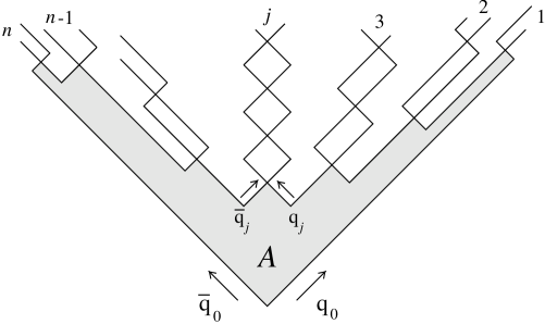
Figure 5: The break-up of a Lund string.

The constant force field spanned between a colour-$3$ quark and a colour-$\overline{3}$ anti-quark is a simple mode of the massless relativistic string. The process has been generalised into a situation with multigluon emission in [12] using the Lund interpretation that the gluons are internal excitations on the string field.

The area decay law in Eq.(20) can be implemented as an iterative process, in which the particles are produced in a stepwise way ordered along the positive (or negative) light-cone. If a set of hadrons is generated, each one takes a fraction $z$ of the remaining light-cone component $E+p_{l}$ (or $E-p_{l}$, if they are generated along the negative light-cone), with $z$ given by the distribution

$$f(z)=N\frac{(1-z)^{a}}{z}\exp(-bm_{\perp}^{2}/z).$$ (21)

The parameters $N$, $a$ and $b$ are related by normalisation, leaving two free parameters. The transverse mass parameter in the fragmentation function is $m_{\perp}^{2}=m^{2}+\vec{p}_{\perp}^{\,2}$, with the transverse momentum obtained as the sum of the transverse momenta stemming from the q and $\overline{\mbox{q}}$ particles generated at the neighbouring vertices, $\vec{p}_{\perp}=\vec{k}_{\perp 2}-\vec{k}_{\perp 1}$. In the Lund model a $\mbox{q}\overline{\mbox{q}}$-pair with transverse momenta $\pm k_{\perp}$ is produced through a quantum mechanical tunneling process. It results in a Gaussian distribution for the transverse momenta

$$d^{2}k_{\perp}\exp(-\pi k_{\perp}^{2}/\kappa).$$ (22)

The whole process is implemented in the Monte Carlo program JETSET [8].

Consider the production of a particle with transverse mass $m_{\perp}$. Given that one vertex has the rapidity $y_{1}$, the rapidity difference $\Delta y$ is not enough to specify the position of the other vertex. One must also know the proper-time of the first vertex. This is shown in energy-momentum space in Fig.6 where the first vertex is specified by $\Gamma$ which is the squared product of the proper-time and $\kappa$.

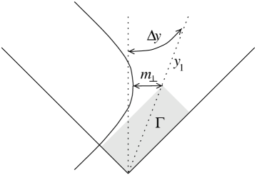
Figure 6: The longitudinal energy scale in the Lund model is $\langle\Gamma\rangle$. The figure shows the production of a particle with transverse mass $m_{\perp}$. The difference in rapidity between the constituent vertices has to be related to the $\Gamma$ of one of the vertices in order for the vertices to be specified.

Of course there are two solutions in this case, but one is strongly favoured by the area dependence in Eq.(20). In the Lund model the vertices, on average, lie on a hyperbola given by a typical $\Gamma$. That is to say, the steps in rapidity in the particle production are related to the scale $\langle\Gamma\rangle$ as given by the model. There is a similar situation in the transverse momentum generation. The squared transverse momentum of a particle is not only given by the azimuthal angle $\Delta\phi$ between the break-up points that generate the particle. The lengths of the transverse momenta of the q and the $\overline{\mbox{q}}$ that make up the particle are also needed. In the tunneling process in Eq.(22) these sizes are given by the scale $\kappa/\pi$.

Thus the Lund fragmentation model provides two different energy scales; one longitudinal to relate to the rapidity difference between vertices and one transverse to relate to their difference in azimuthal angle.

6.2 A modified fragmentation process with screwiness

The main idea in the screwiness model is that the transverse momentum of the emitted particles stems from the piece of screwy gluon field that is in between the two break-up points producing the particle. Therefore we begin by summing up the transverse momentum that is emitted between two points along the field line, cf. Eq.(5):

$$\int^{2}_{1}\frac{\vec{dk}_{\perp}}{d\phi}d\phi=\vec{k}_{\perp 2}-\vec{k}_{\perp 1}=m\tau[\vec{e}_{\perp 1}(\phi_{2})-\vec{e}_{\perp 1}(\phi_{1})].$$ (23)

Figure 7: A $\mbox{q}\overline{\mbox{q}}$-pair is produced in a break-up point with azimuthal angle $\phi$. The figure illustrates how the screwy gluon field between $\phi_{1}$ and $\phi_{2}$ is associated with the transverse momentum ($-k_{\perp 1},k_{\perp 2}$) of the quarks produced at the two break-up points. This association has the property that the produced transverse momentum is conserved locally in each break-up point.

We note that the quantity $m\tau$ also occurs here. We will always consider the parameter $m$ to be a suitable fixed mass parameter but according to the assumed wave function for the current the direction $\tau$ may vary between the different break-up points. To keep the presentation clear we will start off keeping $\tau$ fixed. In the end we will present the generalisation to the case of a varying $\tau$.

If we associate $\pm\vec{k}_{\perp i}$ with the transverse momenta of the $\mbox{q}\overline{\mbox{q}}$-pair produced at vertex $i$, the transverse momenta of the produced particles are given by Eq.(23). The corresponding squared transverse momentum is then

$$p^{2}_{\perp i}=2m^{2}\tau^{2}[1-\cos(\Delta\phi)]$$ (24)

where $\Delta\phi=\phi_{i}-\phi_{i-1}$. Since $\Delta\phi$ is proportional to the rapidity difference between vertices $\Delta y$, it can be written as a function of the particle’s light-cone fraction $z$

$$\Delta\phi=\frac{\Delta y}{\tau}=\frac{1}{2\tau}\log\left(\frac{z+m^{2}_{\perp}/\Gamma}{z(1-z)}\right)$$ (25)

where $\Gamma$ is defined as in Fig.6 and with respect to the previous break-up point $i-1$. Taken together this means that we can write the transverse momentum of a particle as a function of $z$ and $\tau$

$$p^{2}_{\perp}(z)=2m^{2}\tau^{2}\left[1-\cos\left(\frac{\Delta y(z)}{\tau_{i}}\right)\right].$$ (26)

As explicitly manifested in Eq.(26) this means that the transverse and longitudinal components are connected in this model. Inserting $p^{2}_{\perp}(z)$ in the Lund fragmentation function gives

$$f(z)=N\frac{(1-z)^{a}}{z}\exp\left(-\frac{b}{z}\left(m^{2}_{h}+p^{2}_{\perp}(z)\right)\right).$$ (27)

In this way Eq.(27) gives the distribution of light-cone fractions for a given direction $\tau$.

This model keeps the longitudinal properties of the ordinary Lund fragmentation model, but the azimuthal properties are changed. Rapidity differences are still related to $\langle\Gamma\rangle$ but steps in the azimuthal angle are now correlated with steps in rapidity. The azimuthal angles are no longer related to $\kappa/\pi$ as given by the tunneling process, but instead to $m^{2}\tau^{2}$ as given by the screwy gluon field.

When going from one vertex to the next in the case of varying $\tau$ one has to keep in mind that the transverse momentum produced at the first vertex has been specified by the previous step. In order to conserve the transverse momenta generated at each vertex we therefore modify the association in Eq.(23), as follows

$$\int^{i}_{i-1}\frac{\vec{dk}_{\perp}}{d\phi}d\phi=\vec{k}_{\perp i}-\frac{\tau_{i}}{\tau_{i-1}}\vec{k}_{\perp i-1}$$ (28)

where $\tau_{i}$ denotes the direction between break-up points $i-1$ and $i$, cf. Fig.7. The transverse momenta of the produced particles are then given by

$$\vec{p}_{\perp i} = \vec{k}_{\perp i}-\vec{k}_{\perp i-1}=m\left[\tau_{i}\vec{e}_{\perp 1}(\phi_{i})-\tau_{i-1}\vec{e}_{\perp 1}(\phi_{i-1})\right],$$

$$p^{2}_{\perp i} = m^{2}\left[\tau^{2}_{i}+\tau^{2}_{i-1}-2\tau_{i}\tau_{i-1}\cos(\Delta\phi)\right].$$ (29)

The $p_{\perp}^{2}$ given by Eq.(29) can then be put into the fragmentation function. Varying $\tau$ results in larger variations in the emitted transverse momenta of the particles. We have used a Gaussian distribution of $\tau$-directions and we have approximated $m_{\perp}^{2}$ in Eq.(25) with $m_{\perp}^{2}\simeq m_{h}^{2}+\langle p_{\perp min}^{2}\rangle=m_{h}^{2}+2m^{2}\sigma^{2}_{\tau}$. Where $m_{h}$ is the hadron mass and $\sigma_{\tau}$ denotes the width in the distribution of $\tau$-directions. The equations can be solved iteratively without this approximation, but we find that our results are unaffected by this approximation.

7 Is screwiness observable?

In this section we will address the question of whether introducing a correlation between $y$ and $\phi$ of the string break-up vertices has observable consequences for the produced particles. There are two processes which in principle can destroy such a correlation. Firstly, there is the initial particle production and secondly, there are resonance decays. The initial particle production spoils things because even if the vertices lie on a perfect helix the produced particle will usually not lie on the line between its two constituent vertices in the $(y,\phi)$-plane. The particle production fluctuations are mainly in rapidity, i.e. a particle is produced with an azimuthal angle which roughly corresponds to the average angle of its constituent vertices, while its rapidity is distributed with width unity around the average of the vertices.

To study the consequences of the screwiness model we have generated events with three different values $\langle\tau\rangle=0.3,0.5~{}\mbox{and}~{}0.7$. For each value we have tuned the parameters of the model to agree with the multiplicity, rapidity and transverse momentum distributions of default JETSET. In this way we can study the correlations introduced by the model as compared to the ordinary Lund string model. We have tuned $m$ to get the default average $p_{\perp}$ of the produced particles, utilizing the fact that the product $m\tau$ is the important factor. The parameter $b$ has been changed from the default JETSET value to tune the multiplicity, and $\sigma_{\tau}$ has been tuned to get the final charged $p_{\perp}$ fluctuations. Tuning with different $\langle\tau\rangle$ values results in the parameter values shown in Table 1.

$\langle\tau\rangle$	0.3	0.5	0.7
$m$	1.0	0.71	0.61
$b$	0.64	0.68	0.7
$\sigma_{\tau}$	0.2	0.3	0.35

Table 1: Parameter values. The model has been tuned to the multiplicity and charged final $p_{\perp}$ distributions of default JETSET ($b=0.58$).

We note in particular that to get the multiplicity distributions of default JETSET only minor changes of the $b$-parameter are needed. We also note that the restriction in Eq.(19) is satisfied for all the cases since in this model only a fraction of the energy available in the Lund string is used to produce transverse momenta.

We have generated pure $\mbox{q}\overline{\mbox{q}}$ events and the particles in the central rapidity plateau have been included in the analysis. The plots shown are for four units of rapidity, but the qualitative results for observable screwiness are unaffected for values as low as approximately three units of central rapidity. We have analysed the properties of the generated events by means of the screwiness measure, defined in Eq.(13). Here, the second sum in the measure instead goes over the hadrons or over the break-up vertices. The weight $P_{e}$ is of course unity for all events.

In Fig.8 the screwiness for the break-up vertices is shown. It has a clear peak for the different values of $\langle\tau\rangle$, and the $\omega$-values for the peaks correspond to the average $\tau$ values used.

Figure 8: Screwiness for the string break-up vertices. The three curves shown are for $\langle\tau\rangle=0.3,~{}0.5~{}\mbox{and}~{}0.7$, respectively. There is a clear peak at $\omega\simeq 1/\langle\tau\rangle$ in all the cases.

The screwiness for the initially produced particles is shown in Fig.9. We note that the peak vanishes for small values of $\tau$. A helix where the windings are separated by two units of rapidity corresponds to $\tau=1/\pi$. The vanishing of the signal for small $\tau$ values is therefore in agreement with our findings for the rapidity fluctuations in the particle production.

Figure 9: Screwiness for the directly produced particles. The three solid curves are for $\langle\tau\rangle=0.3,~{}0.5~{}\mbox{and}~{}0.7$, respectively. The peak decreases as $\langle\tau\rangle$ is reduced. For $\langle\tau\rangle=0.3$ the peak has vanished due to the fluctuations in particle production. The screwiness for default JETSET (dashed line) has been included for comparison.

For comparison we have included the screwiness for the initial particles produced by default JETSET in Fig.9. As expected no signal is found in this case. The screwiness is further diluted by resonance decays, but it is still visible for not too small $\tau$ values as shown in Fig.10.

To try to enhance the signal we have investigated how the screwiness measure depends on multiplicity and the transverse momentum of the particles. Selecting events with large initial multiplicity enhances the signal. However, analysing events with different final multiplicities separately does not give an enhancement of the signal. The influence of resonance decays on the multiplicity is too large.

Selecting events where $\langle p^{2}_{\perp}\rangle$ is large enhances the signal when decays are not included. This is shown for $\langle\tau\rangle=0.3$ in the left part of Fig.11 where events with $\langle p_{\perp}^{2}\rangle>0.3$ GeV² for the initial particles have been selected. As shown in the figure this event selection results in the signal surviving particle production even for small $\langle\tau\rangle$-values. This event selection is also profitable when it comes to decreasing the effects of resonance decays since events with many decay products are not likely to be selected. In the right part of Fig.11 we show the screwiness for the final state particles in events where $\langle p_{\perp}^{2}\rangle>0.25$ GeV². The curves shown are for $\langle\tau\rangle=0.3$ to show that with event selection a signal can be obtained even for this case. Using the same event selection of course enhances the signal for larger $\langle\tau\rangle$-values, but in those cases it was clearly visible in the total sample.

Figure 10: Screwiness for the final particles ($\pi^{0}$’s are set stable). The three curves shown are for $\langle\tau\rangle=0.3,~{}0.5~{}\mbox{and}~{}0.7$, respectively. For not too small $\langle\tau\rangle$-values there is a peak at $\omega\simeq 1/\langle\tau\rangle$.

Figure 11: Screwiness for $\langle\tau\rangle=0.3$. To enhance the signal events where $\langle p_{\perp}^{2}\rangle$ is large have been selected (solid lines). We have included the corresponding curve with no event selection (dashed lines) to indicate the improvement. Left) Initially produced particles. $\langle p_{\perp}^{2}\rangle>0.3~{}\mbox{GeV}^{2}$. Right) The final particles. $\pi^{0}$’s are set stable. $\langle p_{\perp}^{2}\rangle>0.25~{}\mbox{GeV}^{2}$.

A total of 50000 $\mbox{q}\overline{\mbox{q}}$ events have been used in the analysis, except in the event selection analysis in Fig.11 where 250000 events are analysed. To be able to observe screwiness for such a small $\langle\tau\rangle$-value one needs to increase the number of events by a factor of about five compared to the larger values. Since we have only used positive $\langle\tau\rangle$-values, events with a preferred rotational direction are generated. We could have included both rotational directions in the event generation which would add a signal for negative $\omega$, but reduce the statistics by a factor of two.

The effects on the screwiness from hard gluons stemming from the parton cascade will be investigated in future work. However, since only a fairly small number of events are needed for the results in this paper we expect that investigations of experimental data, in which hard gluon activity is excluded, can be profitable.

A specific property of our model is that $\langle p_{\perp}^{2}\rangle$ for directly produced pions is smaller than $\langle p_{\perp}^{2}\rangle$ for heavier particles. This feature appears to be in agreement with experimental data on two-particle correlations [13]. A model for correlations in $p_{\perp}$ in the string hadronization process with similar consequences was introduced in [14]. The $p_{\perp}$ for directly produced pions and $\rho$’s are shown for the screwiness model in Fig.12 and the distributions are clearly different. In the figure we also show the $p_{\perp}$ distribution of the final pions and compare it to the default JETSET distribution. As seen the secondary pions wash out the differences. The $\langle p_{\perp}\rangle$ for various flavours at the initial production level depend on the screwiness parameters, but the qualitative difference remains.

Figure 12: Left) The $p_{\perp}$ (GeV) distributions for the directly produced $\pi$’s (solid) and $\rho$’s (dashed). The curves shown are for $\tau=0.5$. Right) The $p_{\perp}$ (GeV) distributions for the all final pions (solid), $\pi^{0}$’s are set stable, as compared with default JETSET (dashed).

8 Conclusions

It is perhaps surprising that such an ordered structure as a helix could emerge at the end of the QCD cascade. However, when we consider the constraint imposed by helicity conservation, we see that purely random configurations of gluons are disfavoured. This is because the exclusion region around each gluon restricts the maximum number of allowed gluons. Instead we see that the gluons can achieve the maximum concentration by close packing themselves into the form of a helix. The fragmentation of this screwy field has consequences for the final state particles. Although the fragmentation cannot be described in terms of gluon excitations of the Lund string, we have instead modified the Lund fragmentation scheme. If the winding is within reasonable limits then we expect “screwiness” to be an observable feature of the QCD cascade.

Acknowledgments
We thank Patrik Edén for very many valuable discussions. This work was supported in part by the EU Fourth Framework Programme ‘Training and Mobility of Researchers’, Network ‘Quantum Chromodynamics and the Deep Structure of Elementary Particles’, contract FMRX-CT98-0194 (DG 12 - MIHT).

Appendix A Problems with fragmenting soft gluons

In section 4 we claimed that the helix colour-field cannot be implemented as an excited string, since gluons softer than $k_{\perp 0}=1.6$ GeV cannot be considered as excitations of the string.

To illustrate the problems with fragmentation of soft gluons we have investigated JETSET fragmentation of parton configurations with soft gluons emitted according to the Dipole Cascade Model as implemented in the ARIADNE Monte Carlo [15]. The allowed $k_{\perp}$ range for emissions from the colour dipoles is normally between an upper value, given by phase-space limits, and a lower infra-red cut-off, $k_{\perp c}$. We have instead used a small maximum allowed $k_{\perp}$ value (denoted $k_{\perp\mbox{\scriptsize max}}$) to restrict the hardness of the emitted gluons. This soft cascade has been applied to $\mbox{q}\overline{\mbox{q}}$-dipoles oriented along the $z$-axis. The soft gluons have a negligible impact on the event topology and for our purposes it therefore makes sense to define rapidity with respect to the $z$-axis. We have analysed the resulting hadrons in the central rapidity plateau of the events. To emphasize the features of fragmentation of soft gluons we have not included resonance decays in our analysis.

In Fig.13 we show how the average and the squared width of the central multiplicity distribution depend on $k_{\perp\mbox{\scriptsize max}}$.

Figure 13: The multiplicity in central rapidity per unit of rapidty $n$ and the corresponding variance $\sigma_{n}^{2}$ depends on the upper cut-off in the cascade $k_{\perp\mbox{\scriptsize max}}$ (GeV) as shown. Default JETSET has been used for fragmentation and $\sigma_{n}^{2}/n$ does not start to increase until $k_{\perp\mbox{\scriptsize max}}$ is roughly 1.6 GeV

The effect of the soft gluons is an increase of the average multiplicity while the multiplicity fluctuations remain constant or even decrease until $k_{\perp\mbox{\scriptsize max}}$ is above $k_{\perp 0}$. The $\langle p_{\perp}\rangle$ with respect to the $z$-axis of the hadrons only increases from 0.46 GeV for a flat string with no gluon excitations to 0.56 GeV for $k_{\perp\mbox{\scriptsize max}}=3$ GeV. Changing the generated $\langle p_{\perp}\rangle$ by such a small factor has a minor effect ($\sim 5\%$) on the average multiplicity in pure $\mbox{q}\overline{\mbox{q}}$ events whilst adding the soft gluons increases the average multiplicity by roughly $40\%$, as shown in the figure. As mentioned in section 4, we find that the soft gluons essentially only increase the hadron multiplicity. The number of gluons per rapidity unit varies from 0.25 for $k_{\perp\mbox{\scriptsize max}}=1$ GeV to 0.7 for $k_{\perp max}=5$ GeV. The situation is even worse in the case of the helix field where the expected number of soft gluons per unit of rapidity is significantly larger. We conclude that gluons softer than $k_{\perp 0}$ cannot be implemented inside the Lund Model as individual gluonic excitations of the string.

We will end this appendix with an interpretation of the Lund fragmentation model, which provides us with the possibility to relate $k_{\perp 0}$ to the $b$-parameter in the model. The result in Eq.(20) (although derived semi-classically) can be interpreted quantum-mechanically by a comparison to Fermi’s Golden Rule. It equals the final state phase space times the square of a transition matrix element $|{\cal M}|^{2}=\exp(-bA)$. There are two such quantum-mechanical processes, Schwinger tunneling and the Wilson loop integrals, which can be used in this connection (and they result in very similar interpretations of the parameters). For the Schwinger tunneling case we note that if a constant ($\kappa$) force field is spanned across the longitudinal region $X$ during the time $T$ with a transverse size $A_{\perp}$ then the persistence probability of the vacuum (i.e. the probability that the vacuum should not decay by the production of new quanta) is [16]

$$|{\cal M}|^{2}=\exp(-\kappa^{2}XTA_{\perp}\Pi)\;\;.$$ (30)

Here the number $\Pi$ only depends upon the properties of the quanta coupled to the field; for two massless spin $1/2$ flavours it is $\Pi=1/12\pi$. Comparing the result in Eq.(30) to Eq.(20) we find that the parameter $b=A_{\perp}/24\pi$ (taking into account that the Lund model area is counted in lightcone units). From Eq.(4) we obtain the minimum transverse size of the field from which it then follows that the $b$-parameter in the Lund model must be $b\geq\pi/24\kappa\simeq 0.6$ GeV^-2. This is evidently just in accordance with the phenomenological findings in the Lund model for the parameter $b$. Further, considering the distribution in Eq.(22) for the transverse momentum of a produced $\mbox{q}\overline{\mbox{q}}$-pair breaking the string we recognise the quantity $\ell_{min}^{2}$ in the exponential fall-off. We may conclude that there is a wave-function for the Lund string in transverse space with just the right transverse size to allow the “ordinary” transverse fluctuations in momenta.

References

- [1] R.K. Ellis, D.A.Ross and A.E. Terrano, Nucl. Phys. B178, 421 (1981)
-
[2]
Ya.I. Azimov, Yu.L. Dokshitzer, V.A. Khoze and S.I. Troyan,
Phys. Lett. B165, 147 (1985) - [3] B. Andersson, G. Gustafson and C. Sjögren, Nucl. Phys. B380, 391 (1992)
-
[4]
G. Gustafson, Nucl. Phys. B175, 453 (1986)
G. Gustafson and U. Pettersson, Nucl. Phys. B306, 746 (1988) - [5] G. Gustafson, Nucl. Phys. B392, 251 (1993)
- [6] B. Andersson, G. Gustafson and J. Samuelsson, Nucl. Phys. B463, 217 (1996)
- [7] G. Marchesini, B.R. Webber, Nucl. Phys. B238, 1 (1984)
- [8] T. Sjöstrand, Comp. Phys. Comm. 92, 74 (1994)
- [9] N.K. Nielsen, Nucl. Phys. B167, 249 (1980)
- [10] B. Andersson, G. Gustafson, M. Ringnér and P. Sutton, LU TP 98-15, (1998)
- [11] B. Andersson, G. Gustafson and B. Söderberg, Z. Phys. C20, 317 (1983)
- [12] T. Sjöstrand, Nucl. Phys. B248, 469 (1984)
- [13] TASSO coll. W. Braunschweig et. al., Phys. Lett. B231, 548 (1989)
- [14] B. Andersson, G. Gustafson and J. Samuelsson, Z. Phys. C64, 653 (1994)
- [15] L. Lönnblad, Comp. Phys. Comm. 71, 15 (1992)
-
[16]
J. Schwinger, Phys. Rev. 82, 664 (1951)
N.K. Glendenning and T. Matsui, Phys. Rev. D28, 2890 (1983)