MPI-H-V44-1997

A new rigorous light-cone path integral approach to the Landau-Pomeranchuk-Migdal effect in QED and QCD is discussed. The rate of photon (gluon) radiation by an electron (quark) in a medium is expressed through the Green’s function of a two-dimensional Schrödinger equation with an imaginary potential. In QED this potential is proportional to the dipole cross section for scattering of $e^{+}e^{-}$ pair off an atom, in QCD it is proportional to the cross section of interaction of the color singlet quark-antiquark-gluon system with a medium constituent. In QED our predictions agree well with the photon spectrum measured recently at SLAC for 25 GeV electrons. In QCD for a sufficiently energetic quark produced inside a medium we predict the radiative energy loss $\Delta E_{q}\propto L^{2}$, where $L$ is the distance passed by the quark in the medium. It has a weak dependence on the initial quark energy $E_{q}$. The $L^{2}$ dependence transforms into $L^{1}$ as the quark energy decreases. We also give new formulas for nuclear shadowing in hard reactions.

E-mail: bgz@landau.ac.ru

1 Introduction

In 1953 Landau and Pomeranchuk [1] predicted within classical electrodynamics that multiple scattering can considerably suppress bremsstrahlung of high energy charged particles in a medium. In the high energy limit they obtained the photon radiation rate $\propto 1/\sqrt{\omega}$ ($\omega$ is the photon frequency), which differs drastically from the spectrum for an isolated atom $\propto 1/\omega$. Later, this result was confirmed by Migdal [2], who developed a quantum-mechanical theory of this phenomenon. The physical mechanism behind the suppression of the radiation rate in a medium is the loss of coherence for photon emission from different parts of the charged particle trajectory at the scale of the photon formation length.

Since the studies by Landau and Pomeranchuk [1] and Migdal [2], the suppression of radiation processes in medium, called in the current literature the Landau-Pomeranchuk-Migdal (LPM) effect, has been studied in many theoretical papers [3-21]. However, only recently the first quantitative measurement of the LPM effect for high energy electrons was performed at SLAC [22]. Altogether, this experiment corroborated LPM suppression of bremsstrahlung. Unfortunately, contamination of the SLAC data by multiphoton emission makes it difficult to perform an accurate comparison with the theoretical predictions in the entire range of photon energies. Nonetheless, the experimental spectrum for a thin gold target at photon energies from 5 MeV up to 500 MeV for 25 GeV electron beam, where the multiphoton emission gives a small contribution, agrees with predictions of Ref. [15]. The calculations of Ref. [15] were carried out within a new light-cone path integral approach to the LPM effect which we developed in Ref. [14]. In Ref. [15] the radiation rate was calculated including inelastic processes and treating rigorously the Coulomb effects. In all previous analyses the inelastic processes were neglected, and the Coulomb effects were treated in the leading-log approximation. This approximation works well in the limit of strong LPM suppression in an infinite medium. However, it is not good for real situations because of the uncertainty in the value of the Coulomb logarithm.

The approach of Ref. [14] is also applicable in QCD. Analysis of the LPM effect in QCD is of great importance for understanding the longitudinal energy flow in soft and hard hadron-nucleus collisions and the energy loss of a fast quark produced in deep inelastic scattering on nuclear target. It becomes especially interesting in connection with the forthcoming experiments on high energy $AA$-collisions at RHIC and LHC, where the formation of quark-gluon plasma (QGP) is expected. The energy loss of high-$p_{\perp}$ jets produced at the initial stage of $AA$-collision may be an important potential probe for formation of QGP. The first attempt to estimate the radiative quark energy loss $\Delta E_{q}$ in QGP was made by Gyulassy and Wang [10]. They modelled QGP by a system of static scattering centers described by the Debye screened Coulomb potential $\propto\exp(-r\mu_{D})/r$, where $\mu_{D}$ is the color screening mass. The authors studied emission of soft gluons in the region of small transverse momenta $k_{\perp}<<\mu_{D}$, which, however, gives a negligible contribution to $\Delta E_{q}$. Analysis of soft gluon radiation without a restriction on the gluon transverse momentum in the limit of strong LPM suppression within the Gyulassy-Wang (GW) model was performed in Refs. [11, 20]. A similar analysis for cold nuclear matter was given in Ref. [17]. However, the authors of Refs. [11, 17, 20] used some unjustified approximations. For instance, the quark-gluon system emerging after gluon emission was treated as a pointlike color triplet object. A rigorous quantum treatment of the induced gluon radiation was given for the first time in Ref. [14] (see also [21]).

In the present paper we discuss the LPM effect in QED and QCD within the approach of Ref. [14]. We give special attention to technical details omitted in our previous short publications. We also consider from the viewpoint of LPM suppression nuclear shadowing in hard reactions. New formulas for shadowing that take into account the parton transverse motion are derived.

The presentation is organized as follows. Section 2 is devoted to the LPM effect in QED. Using the unitarity of scattering matrix we express the cross section of photon emission through radiative correction to the transverse electron propagator. It is calculated within time-ordered perturbation theory (PT) in coordinate representation. The radiation rate is expressed through the Green’s function of a two-dimensional Schrödinger equation with an imaginary potential which is proportional to the dipole cross section for scattering of $e^{+}e^{-}\gamma$ state off an atom. We demonstrate that the cross section of photon emission can be written in the form analogous to the Glauber amplitude for elastic hadron-nucleus scattering. This representation allows one to view LPM suppression as an absorption effect for $e^{+}e^{-}\gamma$ system. We compare the theoretical predictions with the data of the SLAC experiment [22]. In section 3 we discuss the LPM effect in QCD. As in QED, the radiation rate is expressed through the Green’s function of a two-dimensional Schrödinger equation. The corresponding imaginary potential is proportional to the total cross section for a three-body quark-antiquark-gluon state. We evaluate the quark energy loss for cold nuclear matter and QGP using the oscillator parametrization for the imaginary potential. For a high energy quark incident on a nucleus we predict $\Delta E_{q}\sim 0.1E_{q}(L/10\,\mbox{fm}$). For a fast quark produced inside a medium we obtain $\Delta E_{q}\propto L^{2}$ ($L$ is the quark path length in the medium) while at sufficiently small energy $\Delta E_{q}\propto L$. In section 4 we discuss the LPM effect for hard reactions on nuclear targets. We demonstrate that our approach to the LPM effect can be used for an accurate evaluation of nuclear shadowing. In section 5 we summarize our results.

2 The LPM effect in QED

2.1 General expression for the radiation rate

We begin with the LPM effect for bremsstrahlung of a fast electron. We consider an electron incident on an amorphous target of a finite thickness. Multiphoton emission will be neglected. The probability of photon emission, $P_{\gamma}$, is connected with the probability $P_{e}$ to detect in the final state one electron by the unitarity relation:

$$P_{e}+P_{\gamma}=1\,.$$ (1)

In the absence of interaction of the electron with the quantum photon field, we have $P_{e}=1$. Consequently, Eq. (1) can be rewritten as

$$P_{\gamma}=-\left(\delta P_{e}-\delta P_{e}^{vac}\right)\,,$$ (2)

where $\delta P_{e}$ is the radiative correction of order $\alpha$ ($\alpha=1/137$) to $P_{e}$. On the right-hand side of Eq. (2) we subtracted the vacuum term, which takes into account the renormalization of the electron wave function for initial and final electron states.

We will evaluate $\delta P_{e}$ in time-ordered PT [23, 24]. The corresponding matrix element is generated by transitions $e\rightarrow e^{\prime}\gamma\rightarrow e$. In a medium the electron transverse momentum is not conserved. For this reason it is convenient to use the coordinate representation of time-ordered PT in which the transitions $e\rightarrow e^{\prime}\gamma\rightarrow e$ will reveal themselves through the radiative correction to the electron wave function. Let us first consider the wave function of a fast electron neglecting interaction with the quantum photon field. In the vacuum the radiative-correction-free wave function of a relativistic electron with longitudinal momentum $p_{z}>>m_{e}$ ($m_{e}$ is the electron mass) can be written as

$$\psi(t,\mbox{{\bf r}})=\exp[-ip_{z}(t-z)]\phi(t,\mbox{{\boldmath$\rho$}})\,,$$ (3)

where $\mbox{{\bf r}}=(z,\mbox{{\boldmath$\rho$}})$, and the time-dependence of the transverse wave function $\phi(t,\mbox{{\boldmath$\rho$}})$ is governed by the two-dimensional Schrödinger equation

$$i\frac{\partial\phi(t,\mbox{{\boldmath$\rho$}})}{\partial t}={H}\phi(t,\mbox{{\boldmath$\rho$}})\,,$$ (4)

with the Hamiltonian

$${H}=\frac{({\mbox{{\bf q}}}^{2}+m^{2}_{e})}{2\mu_{e}}\,.$$ (5)

Here q is the operator of transverse momentum, and the Schrödinger mass is $\mu_{e}=p_{z}$. Eqs. (3), (4) hold for each helicity state. At high energy the electron propagates nearly along the light-cone $t-z=\mbox{const}$, and in Eq. (4) the variable $t$ can be viewed as the longitudinal coordinate $z$. For this reason, we will henceforth regard the transverse wave function $\phi$ as a function of $z$ and $\rho$. Eq. (4) allows one to write the following relation, connecting $\phi(z,\mbox{{\boldmath$\rho$}})$ at planes $z=z_{1}$ and $z=z_{2}$,

$$\phi(z_{2},\mbox{{\boldmath$\rho$}}_{2})=\int d\mbox{{\boldmath$\rho$}}_{1}K_{e}(\mbox{{\boldmath$\rho$}}_{2},z_{2}|\mbox{{\boldmath$\rho$}}_{1},z_{1})\phi(z_{1},\mbox{{\boldmath$\rho$}}_{1})\,\,,$$ (6)

where

$$K_{e}(\mbox{{\boldmath$\rho$}}_{2},z_{2}|\mbox{{\boldmath$\rho$}}_{1},z_{1})=\frac{\mu_{e}}{2\pi i\Delta z}\exp\left[\frac{i\mu_{e}(\mbox{{\boldmath$\rho$}}_{2}-\mbox{{\boldmath$\rho$}}_{1})^{2}}{2\Delta z}-\frac{im_{e}^{2}\Delta z}{2\mu_{e}}\right]$$ (7)

is the Green’s function of the two-dimensional Hamiltonian (5), with $\Delta z=z_{2}-z_{1}$. At high energies spin effects in interaction of an electron with an atom vanish, and equations analogous to (3) and (6) hold for propagation of an electron through the medium as well. The corresponding propagator can be written in the Feynman path integral form

$$K_{e}(\mbox{{\boldmath$\rho$}}_{2},z_{2}|\mbox{{\boldmath$\rho$}}_{1},z_{1})=\int{\cal D}\mbox{{\boldmath$\rho$}}\exp\left\{i\int dz\left[\frac{\mu_{e}\dot{\mbox{{\boldmath$\rho$}}}^{2}}{2}+e\,U(\mbox{{\boldmath$\rho$}},z)\right]-\frac{im_{e}^{2}\Delta z}{2\mu_{e}}\right\}\,\,,$$ (8)

where $\dot{\mbox{{\boldmath$\rho$}}}=d\mbox{{\boldmath$\rho$}}/dz$, and $U(\mbox{{\boldmath$\rho$}},z)$ is the potential of the medium.

The photon wave function can also be written in the form (3). Using the representation (3) for the electron and photon wave functions, we can obtain for the radiative correction to the transverse electron propagator associated with $e^{\prime}\gamma$ intermediate state

$$\delta K_{e}(\mbox{{\boldmath$\rho$}}_{2},z_{2}|\mbox{{\boldmath$\rho$}}_{1},z_{1})=-\int\limits_{0}^{1}dx\int\limits_{z_{1}}^{z_{2}}d\xi_{1}\int\limits_{\xi_{1}}^{z_{2}}d\xi_{2}\int d\mbox{{\boldmath$\tau$}}_{1}d\mbox{{\boldmath$\tau$}}_{2}g(\xi_{1},\xi_{2},x)$$

$$\times K_{e}(\mbox{{\boldmath$\rho$}}_{2},z_{2}|\mbox{{\boldmath$\tau$}}_{2},\xi_{2})K_{e^{\prime}}(\mbox{{\boldmath$\tau$}}_{2},\xi_{2}|\mbox{{\boldmath$\tau$}}_{1},\xi_{1})K_{\gamma}(\mbox{{\boldmath$\tau$}}_{2},\xi_{2}|\mbox{{\boldmath$\tau$}}_{1},\xi_{1})K_{e}(\mbox{{\boldmath$\tau$}}_{1},\xi_{1}|\mbox{{\boldmath$\rho$}}_{1},z_{1})\,.$$ (9)

Here the indices $e^{\prime}$ and $\gamma$ label the electron and photon propagators for the intermediate $e^{\prime}\gamma$ state. The Schrödinger masses that appear in the Green’s functions $K_{e^{\prime}}$ and $K_{\gamma}$ are $\mu_{e^{\prime}}=(1-x)\mu_{e}$ and $\mu_{\gamma}=x\mu_{e}$, where $x$ is the light-cone fractional momentum of the photon. The vertex operator $g(\xi_{1},\xi_{2},x)$, including all spin effects associated with transitions $e\rightarrow e^{\prime}\gamma\rightarrow e$, is given by

$$g(\xi_{1},\xi_{2},x)=\frac{\alpha[4-4x+2x^{2}]}{4x}\,\mbox{{\bf v}}(\xi_{2})\cdot\mbox{{\bf v}}(\xi_{1})+\frac{\alpha m_{e}^{2}x}{2\mu_{e^{\prime}}^{2}}\,\,,$$ (10)

where

$$\mbox{{\bf v}}(\xi_{i})={\mbox{{\bf v}}}_{\gamma}(\xi_{i})-{\mbox{{\bf v}}}_{e^{\prime}}(\xi_{i})\,,$$

$\mbox{{\bf v}}_{\gamma}$ and $\mbox{{\bf v}}_{e^{\prime}}$ are the transverse velocity operators, which act on the corresponding propagators in Eq. (9). Two terms on the right-hand side of Eq. (10) correspond to the $e\rightarrow e^{\prime}\gamma$ transitions conserving and changing the electron helicity.

Now we have all ingredients necessary for calculating the radiation rate. We consider a target with a density $n(z)$ independent of the impact parameter, and assume that $n(z)$ vanishes as $|z|\rightarrow\infty$. In terms of the transverse Green’s function $K_{e}$ and $\delta K_{e}$ the radiative correction $\delta P_{e}$ can be written as

$$\delta P_{e}=2\mbox{Re}\int d\mbox{{\boldmath$\rho$}}_{1}d\mbox{{\boldmath$\rho$}}_{1}^{\prime}d\mbox{{\boldmath$\rho$}}_{2}\phi(z_{1},\mbox{{\boldmath$\rho$}}_{1})\phi^{*}(z_{1},\mbox{{\boldmath$\rho$}}_{1}^{\prime})\langle\delta K_{e}(\mbox{{\boldmath$\rho$}}_{2},z_{2}|\mbox{{\boldmath$\rho$}}_{1},z_{1})K^{*}_{e}(\mbox{{\boldmath$\rho$}}_{2},z_{2}|\mbox{{\boldmath$\rho$}}_{1}^{\prime},z_{1})\rangle\,,$$ (11)

where $\langle\,...\,\rangle$ means averaging over the states of the target, and the points $z_{1}$ and $z_{2}$ are assumed to be at large distances before and after the target, respectively. The initial electron wave function is normalized by the condition

$$\int d\mbox{{\boldmath$\rho$}}|\phi(z_{1},\mbox{{\boldmath$\rho$}})|^{2}=1\,\,.$$ (12)

For a high energy electron one can neglect the longitudinal momentum transfer associated with the interaction with a medium potential. For this reason the unitarity relation (2) is also valid in the differential form in the light-cone variable $x$. Then, using Eqs. (2), (9) and (11), we can obtain for the radiation rate [we suppress the vacuum term, which will be recovered in the final formula (33)]

$$\frac{dP_{\gamma}}{dx}=2\mbox{Re}\int\limits_{z_{1}}^{z_{2}}d\xi_{1}\int\limits_{\xi_{1}}^{z_{2}}d\xi_{2}\int d\mbox{{\boldmath$\rho$}}_{1}d\mbox{{\boldmath$\rho$}}_{1}^{\prime}d\mbox{{\boldmath$\tau$}}_{1}d\mbox{{\boldmath$\tau$}}_{1}^{\prime}d\mbox{{\boldmath$\tau$}}_{2}d\mbox{{\boldmath$\tau$}}_{2}^{\prime}d\mbox{{\boldmath$\rho$}}_{2}\phi(z_{1},\mbox{{\boldmath$\rho$}}_{1})\phi^{*}(z_{1},\mbox{{\boldmath$\rho$}}_{1}^{\prime})$$

$$\times g(\xi_{1},\xi_{2},x)S(\mbox{{\boldmath$\rho$}}_{2},\mbox{{\boldmath$\rho$}}_{2},z_{2}|\mbox{{\boldmath$\tau$}}_{2},\mbox{{\boldmath$\tau$}}_{2}^{\prime},\xi_{2})M(\mbox{{\boldmath$\tau$}}_{2},\mbox{{\boldmath$\tau$}}_{2}^{\prime},\xi_{2}|\mbox{{\boldmath$\tau$}}_{1},\mbox{{\boldmath$\tau$}}_{1}^{\prime},\xi_{1})S(\mbox{{\boldmath$\tau$}}_{1},\mbox{{\boldmath$\tau$}}_{1}^{\prime},\xi_{1}|\mbox{{\boldmath$\rho$}}_{1},\mbox{{\boldmath$\rho$}}_{1}^{\prime},z_{1})\,,$$ (13)

where

$$S(\mbox{{\boldmath$\rho$}}_{2},\mbox{{\boldmath$\rho$}}_{2}^{\prime},\xi_{2}|\mbox{{\boldmath$\rho$}}_{1},\mbox{{\boldmath$\rho$}}_{1}^{\prime},\xi_{1})=\langle K_{e}(\mbox{{\boldmath$\rho$}}_{2},\xi_{2}|\mbox{{\boldmath$\rho$}}_{1},\xi_{1})K^{*}_{e}(\mbox{{\boldmath$\rho$}}_{2}^{\prime},\xi_{2}|\mbox{{\boldmath$\rho$}}_{1}^{\prime},\xi_{1})\rangle$$ (14)

is the evolution operator for the electron density matrix in the absence of interaction with the photon field, and

$$M(\mbox{{\boldmath$\rho$}}_{2},\mbox{{\boldmath$\rho$}}_{2}^{\prime},\xi_{2}|\mbox{{\boldmath$\rho$}}_{1},\mbox{{\boldmath$\rho$}}_{1}^{\prime},\xi_{1})=\langle K_{e^{\prime}}(\mbox{{\boldmath$\rho$}}_{2},\xi_{2}|\mbox{{\boldmath$\rho$}}_{1},\xi_{1})K_{\gamma}(\mbox{{\boldmath$\rho$}}_{2},\xi_{2}|\mbox{{\boldmath$\rho$}}_{1},\xi_{1})K^{*}_{e}(\mbox{{\boldmath$\rho$}}_{2}^{\prime},\xi_{2}|\mbox{{\boldmath$\rho$}}_{1}^{\prime},\xi_{1})\rangle\,.$$ (15)

In deriving Eq. (13) we used the convolution relation

$$K_{e}(\mbox{{\boldmath$\rho$}}_{2},z_{2}|\mbox{{\boldmath$\rho$}}_{1},z_{1})=\int d\mbox{{\boldmath$\tau$}}_{1}d\mbox{{\boldmath$\tau$}}_{2}K_{e}(\mbox{{\boldmath$\rho$}}_{2},z_{2}|\mbox{{\boldmath$\tau$}}_{2},\xi_{2})K_{e}(\mbox{{\boldmath$\tau$}}_{2},\xi_{2}|\mbox{{\boldmath$\tau$}}_{1},\xi_{1})K_{e}(\mbox{{\boldmath$\tau$}}_{1},\xi_{1}|\mbox{{\boldmath$\rho$}}_{1},z_{1})\,.$$ (16)

Using the path integral representation for the transverse Green’s functions, we can rewrite Eqs. (14), (15) in the form

$$S(\mbox{{\boldmath$\rho$}}_{2},\mbox{{\boldmath$\rho$}}_{2}^{\prime},\xi_{2}|\mbox{{\boldmath$\rho$}}_{1},\mbox{{\boldmath$\rho$}}_{1}^{\prime},\xi_{1})=\int{\cal D}\mbox{{\boldmath$\rho$}}_{e}{\cal D}\mbox{{\boldmath$\rho$}}_{e}^{\prime}\exp\left[\frac{i\mu_{e}}{2}\int d\xi(\dot{\mbox{{\boldmath$\rho$}}}_{e}^{2}-\dot{\mbox{{\boldmath$\rho$}}}_{e}^{\prime 2})\right]\Phi(\{\mbox{{\boldmath$\rho$}}_{e}\},\{\mbox{{\boldmath$\rho$}}_{e}^{\prime}\})\,,$$ (17)

$$M(\mbox{{\boldmath$\rho$}}_{2},\mbox{{\boldmath$\rho$}}_{2}^{\prime},\xi_{2}|\mbox{{\boldmath$\rho$}}_{1},\mbox{{\boldmath$\rho$}}_{1}^{\prime},\xi_{1})=\int{\cal D}\mbox{{\boldmath$\rho$}}_{e^{\prime}}{\cal D}\mbox{{\boldmath$\rho$}}_{\gamma}{\cal D}\mbox{{\boldmath$\rho$}}_{e}\exp\left\{\frac{i}{2}\int d\xi(\mu_{e^{\prime}}\dot{\mbox{{\boldmath$\rho$}}}_{e^{\prime}}^{2}+\mu_{\gamma}\dot{\mbox{{\boldmath$\rho$}}}_{\gamma}^{2}-\mu_{e}\dot{\mbox{{\boldmath$\rho$}}}_{e}^{2})\right.$$

$$\left.-\frac{i(\xi_{2}-\xi_{1})}{L_{f}}\right\}\Phi(\{\mbox{{\boldmath$\rho$}}_{e^{\prime}}\},\{\mbox{{\boldmath$\rho$}}_{e}\})\,\,.$$ (18)

Here we introduced the photon formation length

$$L_{f}=2\mu_{e}\left[\frac{m_{e}^{2}}{1-x}-m_{e}^{2}\right]^{-1}=\frac{2E_{e}(1-x)}{m_{e}^{2}x}\,,$$ (19)

which appears in Eq. (18) owing to the difference between the phases of the wave functions of $e$ and $e^{\prime}$ states. Notice that the value of $L_{f}$, emerging in deriving Eq. (18), agrees with the estimate based on the uncertainty relation $\Delta E\Delta t\sim 1$. In the following we will assume that $L_{f}$ is much larger than the atomic size. The boundary conditions for trajectories in Eq. (17) are $\mbox{{\boldmath$\rho$}}_{e}(\xi_{1,2})=\mbox{{\boldmath$\rho$}}_{1,2}$, $\mbox{{\boldmath$\rho$}}_{e}^{\prime}(\xi_{1,2})=\mbox{{\boldmath$\rho$}}_{1,2}^{\prime}$, and in Eq. (18) $\mbox{{\boldmath$\rho$}}_{e^{\prime},\gamma}(\xi_{1,2})=\mbox{{\boldmath$\rho$}}_{1,2}$, $\mbox{{\boldmath$\rho$}}_{e}(\xi_{1,2})=\mbox{{\boldmath$\rho$}}_{1,2}^{\prime}$. The phase factor $\Phi$ in Eqs. (17) and (18) that takes into account interaction with a medium potential is given by

$$\Phi(\{\mbox{{\boldmath$\rho$}}_{i}\},\{\mbox{{\boldmath$\rho$}}_{j}\})=\left\langle\exp\left\{ie\int d\xi[U(\mbox{{\boldmath$\rho$}}_{i}(\xi),\xi)-U(\mbox{{\boldmath$\rho$}}_{j}(\xi),\xi)]\right\}\right\rangle\,.$$ (20)

Note that this phase factor can be viewed as the one for propagation through the medium of $e^{+}e^{-}$ system. However, it should be borne in mind that the ”positron” kinetic energy term in Eqs. (17), (18) is negative.

We will neglect the correlations in the positions of medium atoms. In this case $\Phi(\{\mbox{{\boldmath$\rho$}}_{i}\},\{\mbox{{\boldmath$\rho$}}_{j}\})$ can be written as

$$\Phi(\{\mbox{{\boldmath$\rho$}}_{i}\},\{\mbox{{\boldmath$\rho$}}_{j}\})=\left\{1-\frac{1}{N}\int d\xi n(\xi)\right.\,\,\,\,\,\,\,\,\,\,\,\,\,\,\,\,\,\,\,\,\,$$

$$\times\left.\int d{\mbox{{\bf b}}}\left\langle 1-\exp\left\{ie\int d\xi^{\prime}[\varphi(\mbox{{\boldmath$\rho$}}_{i}(\xi^{\prime})-{\mbox{{\bf b}}},\xi^{\prime}-\xi)-\varphi(\mbox{{\boldmath$\rho$}}_{j}(\xi^{\prime})-{\mbox{{\bf b}}},\xi^{\prime}-\xi)]\right\}\right\rangle_{a}\right\}^{N}\,\,,$$ (21)

where $\varphi({\bf r})$ is the atomic potential, $N$ is the number of the atoms in the targets, $\langle\,...\,\rangle_{a}$ denotes averaging over the states of the atom. After exponentiating Eq. (21) can be written in the form

$$\Phi(\{\mbox{{\boldmath$\rho$}}_{i}\},\{\mbox{{\boldmath$\rho$}}_{j}\})=\exp\left[-\frac{1}{2}\int d\xi n(\xi)\sigma(|\mbox{{\boldmath$\rho$}}_{i}(\xi)-\mbox{{\boldmath$\rho$}}_{j}(\xi)|)\right]\,\,,$$ (22)

where

$$\sigma(|\mbox{{\boldmath$\rho$}}|)=2\int d{\mbox{{\bf b}}}\left\langle 1-\exp\left\{ie\int d\xi[\varphi(\mbox{{\boldmath$\rho$}}-{\mbox{{\bf b}}},\xi)-\varphi({\mbox{{\bf b}}},\xi)]\right\}\right\rangle_{a}$$ (23)

is the dipole cross section for scattering of $e^{+}e^{-}$ pair of the transverse size $\rho$ on the atom. In arriving at (22) we neglected the variation of $|\mbox{{\boldmath$\rho$}}_{i}(\xi)-\mbox{{\boldmath$\rho$}}_{j}(\xi)|$ at the longitudinal scale on the order of the atomic radius $a$. This is a good approximation for $L_{f}>>a$.

For an atomic potential $\varphi(r)=(Ze/4\pi r)\exp(-r/a)$ ($a\sim r_{B}Z^{-1/3}$, $r_{B}$ is the Bohr radius) $\sigma(\rho)$ in the Born approximation is given by

$$\sigma(\rho)=8\pi(Z\alpha a)^{2}\left[1-\frac{\rho}{a}K_{1}\left(\frac{\rho}{a}\right)\right]\,,$$ (24)

where $K_{1}$ is the Bessel function. For $\rho\ll a$, which will be important in the problem under consideration, we have $\sigma(\rho)\simeq C(\rho)\rho^{2}\,,$ where

$$C(\rho)=4\pi(Z\alpha)^{2}\left[\log\left(\frac{2a}{\rho}\right)+\frac{(1-2\gamma)}{2}\right]\,,\;\;\;\;\gamma=0.577\,.$$ (25)

For nuclei of finite radius $R_{A}$, Eq. (25) holds for $\rho\mathrel{\hbox to0.0pt{\lower 4.0pt\hbox{\hskip 1.0pt$\sim$}\hss}\raise 1.0pt\hbox{$>$}}R_{A}$, and $C(\rho\mathrel{\hbox to0.0pt{\lower 4.0pt\hbox{\hskip 1.0pt$\sim$}\hss}\raise 1.0pt\hbox{$<$}}R_{A})=C(R_{A})$. In section 2.4 we will give a more accurate formula for $C(\rho)$, which will be used in numerical calculations.

The phase factor (22) is independent of $(\mbox{{\boldmath$\rho$}}_{i}+\mbox{{\boldmath$\rho$}}_{j})/2$. This allows one to calculate the path integral (17) analytically. This gives the following result [25]

$$S(\mbox{{\boldmath$\rho$}}_{2},\mbox{{\boldmath$\rho$}}_{2}^{\prime},\xi_{2}|\mbox{{\boldmath$\rho$}}_{1},\mbox{{\boldmath$\rho$}}_{1}^{\prime},\xi_{1})=\left(\frac{\mu_{e}}{2\pi\Delta\xi}\right)^{2}\exp\left\{\frac{i\mu_{e}}{2\Delta\xi}[(\mbox{{\boldmath$\rho$}}_{1}-\mbox{{\boldmath$\rho$}}_{2})^{2}-(\mbox{{\boldmath$\rho$}}_{1}^{\prime}-\mbox{{\boldmath$\rho$}}_{2}^{\prime})^{2}]\right.$$

$$\left.-\frac{1}{2}\int d\xi n(\xi)\sigma(|\mbox{{\boldmath$\tau$}}_{s}(\xi)|)\right\}\,,$$ (26)

$$\mbox{{\boldmath$\tau$}}_{s}(\xi)=(\mbox{{\boldmath$\rho$}}_{1}-\mbox{{\boldmath$\rho$}}_{1}^{\prime})\frac{(\xi_{2}-\xi)}{\Delta\xi}+(\mbox{{\boldmath$\rho$}}_{2}-\mbox{{\boldmath$\rho$}}_{2}^{\prime})\frac{(\xi-\xi_{1})}{\Delta\xi}\,,\;\;\;\Delta\xi=\xi_{2}-\xi_{1}\,.$$

In the case of the integral (18) we introduce the Jacobi variables $\mbox{{\boldmath$\alpha$}}=(\mu_{e^{\prime}}\mbox{{\boldmath$\rho$}}_{e^{\prime}}+\mu_{\gamma}\mbox{{\boldmath$\rho$}}_{\gamma})/(\mu_{e^{\prime}}+\mu_{\gamma})$ and $\mbox{{\boldmath$\rho$}}=\mbox{{\boldmath$\rho$}}_{e^{\prime}}-\mbox{{\boldmath$\rho$}}_{\gamma}\,$. Then after analytical path integration over $\mbox{{\boldmath$\alpha$}}(\xi)$ and $\mbox{{\boldmath$\rho$}}_{e}(\xi)$ in Eq. (18) we arrive at

$$M(\mbox{{\boldmath$\rho$}}_{2},\mbox{{\boldmath$\rho$}}_{2}^{\prime},\xi_{2}|\mbox{{\boldmath$\rho$}}_{1},\mbox{{\boldmath$\rho$}}_{1}^{\prime},\xi_{1})=\left(\frac{\mu_{e}}{2\pi\Delta\xi}\right)^{2}\exp\left\{\frac{i\mu_{e}}{2\Delta\xi}\left[(\mbox{{\boldmath$\rho$}}_{1}-\mbox{{\boldmath$\rho$}}_{2})^{2}-(\mbox{{\boldmath$\rho$}}_{1}^{\prime}-\mbox{{\boldmath$\rho$}}_{2}^{\prime})^{2}\right]-\frac{i\Delta\xi}{L_{f}}\right\}$$

$$\times\int{\cal D}\mbox{{\boldmath$\rho$}}\exp\left\{i\int d\xi\left[\frac{\mu_{e^{\prime}\gamma}\dot{\mbox{{\boldmath$\rho$}}}^{2}}{2}+i\frac{n(\xi)\sigma(|\mbox{{\boldmath$\tau$}}_{m}(\xi)|)}{2}\right]\right\}\,,$$ (27)

$$\mbox{{\boldmath$\tau$}}_{m}(\xi)=(\mbox{{\boldmath$\rho$}}_{1}-\mbox{{\boldmath$\rho$}}_{1}^{\prime})\frac{(\xi_{2}-\xi)}{\Delta\xi}+(\mbox{{\boldmath$\rho$}}_{2}-\mbox{{\boldmath$\rho$}}_{2}^{\prime})\frac{(\xi-\xi_{1})}{\Delta\xi}+\frac{\mbox{{\boldmath$\rho$}}(\xi)\mu_{\gamma}}{(\mu_{e^{\prime}}+\mu_{\gamma})}\,,$$

where $\mu_{e^{\prime}\gamma}=\mu_{e^{\prime}}\mu_{\gamma}/(\mu_{e^{\prime}}+\mu_{\gamma})=E_{e}x(1-x)$ is the reduced Schrödinger mass of the $e^{\prime}\gamma$ system. It follows from Eqs. (26), (27) that for the factors $S$ and $M$ there hold relations

$$\int d\mbox{{\boldmath$\rho$}}_{2}S(\mbox{{\boldmath$\rho$}}_{2},\mbox{{\boldmath$\rho$}}_{2},\xi_{2}|\mbox{{\boldmath$\rho$}}_{1},\mbox{{\boldmath$\rho$}}_{1}^{\prime},\xi_{1})=\delta(\mbox{{\boldmath$\rho$}}_{1}-\mbox{{\boldmath$\rho$}}_{1}^{\prime})\,,$$ (28)

$$\int d\mbox{{\boldmath$\rho$}}_{2}M(\mbox{{\boldmath$\rho$}}_{2},\mbox{{\boldmath$\rho$}}_{2},\xi_{2}|\mbox{{\boldmath$\rho$}}_{1},\mbox{{\boldmath$\rho$}}_{1}^{\prime},\xi_{1})=\delta(\mbox{{\boldmath$\rho$}}_{1}-\mbox{{\boldmath$\rho$}}_{1}^{\prime}){\cal K}(0,\xi_{2}|0,\xi_{1})\,,$$ (29)

where

$${\cal K}(\mbox{{\boldmath$\rho$}}_{2},\xi_{2}|\mbox{{\boldmath$\rho$}}_{1},\xi_{1})=\int{\cal D}\mbox{{\boldmath$\rho$}}\exp\left\{i\int d\xi\left[\frac{\mu_{e^{\prime}\gamma}\dot{\mbox{{\boldmath$\rho$}}}^{2}}{2}+i\frac{n(\xi)\sigma(|\mbox{{\boldmath$\rho$}}|x)}{2}\right]\right\}$$ (30)

is the Green’s function of a two-dimensional Schrödinger equation with the Hamiltonian

$${\cal H}=\frac{{\mbox{{\bf q}}}^{2}}{2\mu_{e^{\prime}\gamma}}+v(\mbox{{\boldmath$\rho$}},\xi)\,,$$ (31)

$$v(\mbox{{\boldmath$\rho$}},\xi)=-i\frac{n(\xi)\sigma(|\mbox{{\boldmath$\rho$}}|x)}{2}\,.$$ (32)

The Hamiltonian (31) describes the electron-photon relative transverse motion in the $e^{\prime}\gamma$ system. The form of the imaginary potential (32) reflects the fact that after integrating over $\mbox{{\boldmath$\rho$}}_{2}$ in Eq. (29) the ”positron” trajectory $\mbox{{\boldmath$\rho$}}_{e}(\xi)$ coincides with the trajectory of the center-of-mass of the $e^{\prime}\gamma$ system.

Substituting (26), (27) into (13) and integrating in (13) over the transverse variables with the help of (28), (29), along with the normalization condition (12), we finally obtain (we set $-z_{1}=z_{2}=\infty$, and recover the vacuum term)

$$\frac{dP_{\gamma}}{dx}=2\mbox{Re}\int\limits_{-\infty}^{\infty}d\xi_{1}\int\limits_{\xi_{1}}^{\infty}d\xi_{2}\exp\left(-\frac{i\Delta\xi}{L_{f}}\right)g(\xi_{1},\xi_{2},x)\left[{\cal K}(0,\xi_{2}|0,\xi_{1})-{\cal K}_{v}(0,\xi_{2}|0,\xi_{1})\right]\,.$$ (33)

Here ${\cal K}_{v}$ is the Green’s function for the Hamiltonian (31) with $v(\mbox{{\boldmath$\rho$}},\xi)=0$.

Thus, we expressed the intensity of the photon radiation through the Green’s function of the Schrödinger equation with the imaginary potential (32). Notice that the dipole cross section in Eq. (32) can be viewed as an imaginary part of the forward scattering amplitude for the three-body $e^{+}e^{-}\gamma$ system. In our analysis we neglected interaction of the photon with atomic electrons, which becomes important only for extremely soft photons [2, 7]. The inclusion of this interaction leads to appearance of a real part in the potential (32).

It is worth noting that an equation analogous to (33) holds also in more general case of photon emission on a random external potential if the photon formation length is much larger than the potential correlation radius. In this case the integral over $\xi$ in Eq. (20) defines a Gaussian random quantity. Using the formula $\langle\exp(iA)\rangle=\exp(-\langle A^{2}\rangle/2)$, which is valid for a Gaussian random quantity, we find that the phase factor (20) takes the form

$$\Phi(\{\mbox{{\boldmath$\rho$}}_{i}\},\{\mbox{{\boldmath$\rho$}}_{j}\})=\exp\left[-i\int d\xi V\left(\mbox{{\boldmath$\rho$}}_{i}(\xi)-\mbox{{\boldmath$\rho$}}_{j}(\xi),\xi\right)\right]\,,$$ (34)

$$V(\mbox{{\boldmath$\rho$}},\xi)=-2\pi i\alpha\int\limits_{-\infty}^{\infty}d\xi^{\prime}\langle\Delta U(\mbox{{\boldmath$\rho$}},\xi)U(\mbox{{\boldmath$\rho$}},\xi^{\prime})\rangle\,,$$ (35)

where $\Delta U(\mbox{{\boldmath$\rho$}},\xi)=U(\mbox{{\boldmath$\rho$}},\xi)-U(0,\xi)$. The function (35) will play the role of the imaginary potential in the Hamiltonian (31).

2.2 Bremsstrahlung in an infinite medium in the oscillator approximation

To proceed with analytical evaluation of the radiation rate we take advantage of the slow $\rho$-dependence of $C(\rho x)$ at $\rho x\mathrel{\hbox to0.0pt{\lower 4.0pt\hbox{\hskip 1.0pt$\sim$}\hss}\raise 1.0pt\hbox{$<$}}1/m_{e}$, which, as will be seen below, are important in Eq. (33). Evidently, to a logarithmic accuracy we can replace (32) by the harmonic oscillator potential with the frequency

$$\Omega=\frac{(1-i)}{\sqrt{2}}\left(\frac{nC(\rho_{eff}x)x^{2}}{\mu_{e^{\prime}\gamma}}\right)^{1/2}=\frac{(1-i)}{\sqrt{2}}\left(\frac{nC(\rho_{eff}x)x}{E_{e}(1-x)}\right)^{1/2}\,\,.$$ (36)

Here $\rho_{eff}$ is the typical value of $\rho$ for trajectories dominating the radiation rate. Making use of the oscillator Green’s function

$$K_{osc}(\mbox{{\boldmath$\rho$}}_{2},z_{2}|\mbox{{\boldmath$\rho$}}_{1},z_{1})=\frac{\mu\Omega}{2\pi i\sin{(\Omega\Delta z)}}\exp\left\{\frac{i\mu[(\mbox{{\boldmath$\rho$}}_{1}^{2}+\mbox{{\boldmath$\rho$}}_{2}^{2})\cos{(\Omega\Delta z)}-2\mbox{{\boldmath$\rho$}}_{1}\mbox{{\boldmath$\rho$}}_{2}]}{2\sin{(\Omega\Delta z)}}\right\}\,\,,$$ (37)

after some algebra one can obtain from Eq. (33) the intensity of bremsstrahlung per unit length in an infinite medium

$$\frac{dP_{\gamma}}{dxdL}=n\left(\frac{C(\rho_{eff}x)}{C(1/m_{e})}\right)\left[\left(\frac{d\sigma}{dx}\right)^{BH}_{nf}S_{nf}(\eta)+\left(\frac{d\sigma}{dx}\right)^{BH}_{sf}S_{sf}(\eta)\right]\,,$$ (38)

where $\eta=L_{f}|\Omega|$. In Eq. (38) we factored out the Bethe-Heitler cross sections conserving (nf) and changing (sf) the electron helicity, which to a logarithmic accuracy can be written as

$$\left(\frac{d\sigma}{dx}\right)^{BH}_{nf}=\frac{\alpha C(1/m_{e})}{3\pi m_{e}^{2}}\frac{[4-4x+2x^{2}]}{x}\,\,,$$ (39)

$$\left(\frac{d\sigma}{dx}\right)^{BH}_{sf}=\frac{\alpha C(1/m_{e})}{3\pi m_{e}^{2}}\,x\,\,.$$ (40)

The factors $S_{nf}$, $S_{sf}$ in Eq. (38) are given by

$$S_{nf}(\eta)=\frac{3}{\eta\sqrt{2}}\int\limits_{0}^{\infty}dy\left(\frac{1}{y^{2}}-\frac{1}{{\rm sh}^{2}y}\right)\exp\left(-\frac{y}{\eta\sqrt{2}}\right)\left[\cos\left(\frac{y}{\eta\sqrt{2}}\right)+\sin\left(\frac{y}{\eta\sqrt{2}}\right)\right]\,,$$ (41)

$$S_{sf}(\eta)=\frac{6}{\eta^{2}}\int\limits_{0}^{\infty}dy\left(\frac{1}{y}-\frac{1}{{\rm sh}y}\right)\exp\left(-\frac{y}{\eta\sqrt{2}}\right)\sin\left(\frac{y}{\eta\sqrt{2}}\right)\,.$$ (42)

At small $\eta$ $S_{nf}(\eta)\simeq 1-16\eta^{4}/21$, $S_{sf}(\eta)\simeq 1-31\eta^{4}/21$, and the Bethe-Heitler regime obtains. Up to the factor $C(\rho_{eff}x)/C(1/m_{e})$, which is slowly dependent on $\eta$, the suppression of bremsstrahlung at $\eta\gg 1$ is controlled by the asymptotic behavior of the suppression factors (41), (42):

$$S_{nf}(\eta)\simeq 3/\eta\sqrt{2}\,,~{}~{}~{}~{}S_{sf}(\eta)\simeq 3\pi/2\eta^{2}\,.$$ (43)

The value of $\rho_{eff}$ can be estimated with the help of Eqs. (41), (42). The variable of integration in (41), (42) in terms of $\Delta\xi$ in Eq. (33) equals $|\Delta\xi\Omega|$. Therefore, for typical value of $\Delta\xi$ contributing to the integral (33), $\Delta\xi_{eff}$, we have $\Delta\xi_{eff}\sim L_{f}^{{}^{\prime}}={\mbox{ min}}(L_{f},1/|\Omega|)$. Note that $L_{f}^{{}^{\prime}}$ plays the role of the effective medium-modified photon formation length. Having $\Delta\xi_{eff}$ we can estimate $\rho_{eff}$ from the obvious Schrödinger diffusion relation:

$$\rho_{eff}\sim(2\Delta\xi_{eff}/\mu_{e^{\prime}\gamma})^{1/2}\,.$$ (44)

In the low-density limit, when $\eta\rightarrow 0$, this relation yields $\rho_{eff}\sim 1/m_{e}x$, and the right-hand side of Eq. (38) goes over into the Bethe-Heitler cross section times the target density. In the soft photon limit ($x\rightarrow 0$) at fixed $n$, $\eta$ becomes much greater than unity. In this regime of strong LPM suppression, using the asymptotic formula for $S_{nf}$, one can obtain from Eqs. (38), (39)

$$\frac{dP_{\gamma}}{dxdL}\approx 2\alpha^{2}Z\,\sqrt{\frac{2n\log(2a/\rho_{eff}x)}{\pi E_{e}x}}\,,$$ (45)

with $\rho_{eff}\sim\left[\pi(Z\alpha)^{2}nE_{e}x^{3}\log(2/\alpha Z^{1/3})\right]^{-1/4}\,.$ This result agrees with Migdal’s prediction [2] obtained within the Fokker-Planck approximation in the momentum representation. Our suppression factors (41), (42) also agree with those obtained in Ref. [2]. Equivalence of the the oscillator approximation in coordinate representation to the Fokker-Planck one in momentum representation is not surprising. Making use of Eq. (26) one can easily show that $\sigma(\rho)\propto\rho^{2}$ leads to the Gaussian diffusion in the momentum space. That is, we have a diffusion described by the Fokker-Planck equation.

The oscillator approximation simplifies greatly evaluation of the radiation rate. It allows one to obtain simple formulas for suppression factors for a finite-size target as well. The corresponding analysis within Migdal’s approach was performed in Ref. [4]. Unfortunately, the oscillator approximation is accurate only for strong LPM suppression, when one can neglect the variation of the factor $C(\rho)$. This effect must be taken into account to evaluate accurately the radiation rate in an infinite medium in the regime of small LPM suppression and for finite-size targets. In the next section we represent Eq. (33) in a different form which is more convenient for numerical calculations with a rigorous treatment of the Coulomb effects.

2.3 Glauber form of the radiation rate

In this section we demonstrate that Eq. (33) can be rewritten in a form analogous to the Glauber amplitude for elastic hadron-nucleus scattering. Let us expand the Green’s function ${\cal K}$ in Eq. (33) in a series in the potential $v$

$${\cal K}(\mbox{{\boldmath$\rho$}}_{2},z_{2}|\mbox{{\boldmath$\rho$}}_{1},z_{1})={\cal K}_{v}(\mbox{{\boldmath$\rho$}}_{2},z_{2}|\mbox{{\boldmath$\rho$}}_{1},z_{1})\,\,\,\,\,\,\,\,\,\,\,\,\,\,\,\,\,\,\,\,\,\,\,\,\,\,\,\,\,\,\,\,\,\,\,\,\,\,$$

$$\,\,\,\,\,\,\,\,\,\,\,\,\,\,\,\,\,\,\,\,\,\,\,\,+\int\limits_{z_{1}}^{z_{2}}dz\int d\mbox{{\boldmath$\rho$}}{\cal K}_{v}(\mbox{{\boldmath$\rho$}}_{2},z_{2}|\mbox{{\boldmath$\rho$}},z)(-iv(\mbox{{\boldmath$\rho$}},z)){\cal K}_{v}(\mbox{{\boldmath$\rho$}},z|\mbox{{\boldmath$\rho$}}_{1},z_{1})\,+\cdots\,.$$

Then after a simple algebra one can represent (33) in the form

$$\frac{dP_{\gamma}}{dx}=\frac{dP_{\gamma}^{BH}}{dx}+\frac{dP_{\gamma}^{abs}}{dx}\,,$$ (46)

where

$$\frac{dP_{\gamma}^{BH}}{dx}=-T\cdot\mbox{Re}\int d\mbox{{\boldmath$\rho$}}\int\limits_{-\infty}^{0}d\xi_{1}\int\limits_{0}^{\infty}d\xi_{2}g(\xi_{1},\xi_{2},x){\cal K}_{v}(0,\xi_{2}|\mbox{{\boldmath$\rho$}},0)$$

$$\times\sigma(\rho x){\cal K}_{v}(\mbox{{\boldmath$\rho$}},0|0,\xi_{1})\exp\left[-\frac{i(\xi_{2}-\xi_{1})}{L_{f}}\right]\,,$$ (47)

$$\frac{dP_{\gamma}^{abs}}{dx}=\frac{1}{2}\mbox{Re}\int\limits_{0}^{L}dz_{1}n(z_{1})\int\limits_{z_{1}}^{L}dz_{2}n(z_{2})\int d\mbox{{\boldmath$\rho$}}_{1}d\mbox{{\boldmath$\rho$}}_{2}\int\limits_{-\infty}^{z_{1}}d\xi_{1}\int\limits_{z_{2}}^{\infty}d\xi_{2}g(\xi_{1},\xi_{2},x){\cal K}_{v}(0,\xi_{2}|\mbox{{\boldmath$\rho$}}_{2},z_{2})$$

$$\times\sigma(\rho_{2}x){\cal K}(\mbox{{\boldmath$\rho$}}_{2},z_{2}|\mbox{{\boldmath$\rho$}}_{1},z_{1})\sigma(\rho_{1}x){\cal K}_{v}(\mbox{{\boldmath$\rho$}}_{1},z_{1}|0,\xi_{1})\exp\left[-\frac{i(\xi_{2}-\xi_{1})}{L_{f}}\right]\,.$$ (48)

Here $T=\int_{0}^{L}dzn(z)$ is the optical thickness of the target (we assume that $n(z)=0$ at $z<0$ and $z>L$). The integrals over $\xi_{1,2}$ in (47), (48) of the products of the vacuum Green’s functions and exponential phase factors can be expressed through the light-cone wave function $\Psi(x,\mbox{{\boldmath$\rho$}},\lambda_{e},\lambda_{e^{\prime}},\lambda_{\gamma})$ for the transition $e\rightarrow e^{\prime}\gamma$. At $\lambda_{e^{\prime}}=\lambda_{e}$ it is

$$\Psi(x,\mbox{{\boldmath$\rho$}},\lambda_{e},\lambda_{e^{\prime}},\lambda_{\gamma})=\frac{-i}{2\mu_{e^{\prime}\gamma}}\sqrt{\frac{\alpha}{2x}}\left[\lambda_{\gamma}(2-x)+2\lambda_{e}x\right]\left(\frac{\partial}{\partial\rho_{x}}-i\lambda_{\gamma}\frac{\partial}{\partial\rho_{y}}\right)\int\limits_{-\infty}^{0}d\xi{\cal K}_{v}(\mbox{{\boldmath$\rho$}},0|0,\xi)$$

$$\times\exp\left(\frac{i\xi}{L_{f}}\right)=\frac{1}{2\pi}\sqrt{\frac{\alpha x}{2}}\left[\lambda_{\gamma}(2-x)+2\lambda_{e}x\right]\exp(-i\lambda_{\gamma}\varphi)m_{e}K_{1}(\rho m_{e}x)\,,$$ (49)

for $\lambda_{e^{\prime}}=-\lambda_{e}$ the only nonzero component is the one with $\lambda_{\gamma}=2\lambda_{e}$

$$\Psi(x,\mbox{{\boldmath$\rho$}},\lambda_{e},-\lambda_{e},2\lambda_{e})=\frac{\sqrt{2\alpha x^{3}}}{2\mu_{e^{\prime}\gamma}}\int\limits_{-\infty}^{0}d\xi{\cal K}_{v}(\mbox{{\boldmath$\rho$}},0|0,\xi)\exp\left(\frac{i\xi}{L_{f}}\right)=\frac{-i}{2\pi}\sqrt{2\alpha x^{3}}m_{e}K_{0}(\rho m_{e}x)\,.$$ (50)

Here $K_{0}$ and $K_{1}$ are the Bessel functions. Eqs. (49), (50) can be obtained by calculating the matrix element for transition $e\rightarrow e^{\prime}\gamma$ in time-ordered PT using the representation (3) for electron and photon wave functions.

Making use of Eqs. (49), (50) one can rewrite (47), (48) in the form

$$\frac{dP_{\gamma}^{BH}}{dx}=\frac{T}{2}\sum\limits_{\{\lambda_{i}\}}\int d\mbox{{\boldmath$\rho$}}\,|\Psi(x,\mbox{{\boldmath$\rho$}},\{\lambda_{i}\})|^{2}\sigma(\rho x)\,\,,$$ (51)

$$\frac{dP_{\gamma}^{abs}}{dx}=-\frac{1}{4}\mbox{Re}\sum\limits_{\{\lambda_{i}\}}\int\limits_{0}^{L}dz_{1}n(z_{1})\int\limits_{z_{1}}^{L}dz_{2}n(z_{2})\int d\mbox{{\boldmath$\rho$}}\,\Psi^{*}(x,\mbox{{\boldmath$\rho$}},\{\lambda_{i}\})$$

$$\times\sigma(\rho x)\Phi(x,\mbox{{\boldmath$\rho$}},\{\lambda_{i}\},z_{1},z_{2})\exp\left[-\frac{i(z_{2}-z_{1})}{L_{f}}\right]\,,$$ (52)

where

$$\Phi(x,\mbox{{\boldmath$\rho$}},\{\lambda_{i}\},z_{1},z_{2})=\int d\mbox{{\boldmath$\rho$}}^{\prime}{\cal K}(\mbox{{\boldmath$\rho$}},z_{2}|\mbox{{\boldmath$\rho$}}^{\prime},z_{1})\Psi(x,\mbox{{\boldmath$\rho$}}^{\prime},\{\lambda_{i}\})\,\sigma(\rho^{\prime}x)$$ (53)

is the solution of the Schrödinger equation with the boundary condition $\Phi(x,\mbox{{\boldmath$\rho$}},\{\lambda_{i}\},z_{1},z_{1})=\Psi(x,\mbox{{\boldmath$\rho$}},\{\lambda_{i}\})\sigma(\rho x)\,.$

In Ref. [26] it was shown that the $p_{\perp}$-integrated cross section for a radiation process $a\rightarrow bc$ can be written as

$$\frac{d\sigma({a\rightarrow cb})}{dx}=\int d\mbox{{\boldmath$\rho$}}\,W_{a}^{bc}(x,\mbox{{\boldmath$\rho$}})\sigma_{\bar{a}bc}(\rho)\,,$$ (54)

where $W_{a}^{bc}(x,\mbox{{\boldmath$\rho$}})=|\Psi_{a}(x,\mbox{{\boldmath$\rho$}})|^{2}$ is the light-cone probability distribution for transition $a\rightarrow bc$, $\sigma_{\bar{a}bc}$ is the total cross section of interaction with the target of $\bar{a}bc$ system. For the transition $e\rightarrow e^{\prime}\gamma$ the corresponding three-body cross section equals $\sigma(\rho x)$. Consequently, the first term in (46) equals the Bethe-Heitler cross section times the target optical thickness, i.e. it corresponds to the impulse approximation, while the second term describes LPM suppression. Thus, we have demonstrated that LPM suppression is equivalent to absorption for $e^{+}e^{-}\gamma$ system.

It is worth noting that at $L_{f}\gg L$ the radiation rate for a composite target can also be represented in a form similar to that of Eq. (54). Indeed, in this limit the transverse variable $\rho$ is approximately frozen, and the Green’s function can be written in the eikonal form

$${\cal K}(\mbox{{\boldmath$\rho$}}_{2},z_{2}|\mbox{{\boldmath$\rho$}}_{1},z_{1})\approx\delta(\mbox{{\boldmath$\rho$}}_{2}-\mbox{{\boldmath$\rho$}}_{1})\exp\left[-\frac{\sigma(\rho_{1}x)}{2}\int\limits_{z_{1}}^{z_{2}}dz\,n(z)\right]\,.$$ (55)

Using (55) we obtain in the frozen-size approximation from Eqs. (46), (51), (52)

$$\frac{dP_{\gamma}^{fr}}{dx}=2\int d\mbox{{\boldmath$\rho$}}\,W_{e}^{e\gamma}(x,\mbox{{\boldmath$\rho$}})\left\{1-\exp\left[-\frac{T\sigma(\rho x)}{2}\right]\right\}\,.$$ (56)

Eq. (56) is analogous to the formula obtained in Ref. [26] for the cross section of heavy quark production in hadron-nucleus collision. Within classical electrodynamics the LPM effect at $L_{f}\gg L$ was previously discussed in Ref. [13].

Representation (46) has the virtue of bypassing calculation of the singular transverse Green’s function. This renders it convenient for numerical calculations of the radiation rate for finite-size targets.

2.4 Numerical results and comparison with the SLAC experiment

For numerical calculations we need a more accurate parametrization of the dipole cross section, which takes into account the inelastic processes and the Coulomb correction. We write the dipole cross section in the form $\sigma(\rho)=\rho^{2}C(\rho)\,,$ where

$$C(\rho)=Z^{2}C_{el}(\rho)+ZC_{in}(\rho)\,.$$ (57)

Here the terms $\propto Z^{2}$ and $\propto Z$ correspond to elastic and inelastic intermediate states in interaction of $e^{+}e^{-}$ pair with an atom. Due to the steep decrease of the light-cone wave function $\Psi(x,\mbox{{\boldmath$\rho$}},\{\lambda_{i}\})$ at $|\mbox{{\boldmath$\rho$}}|\mathrel{\hbox to0.0pt{\lower 4.0pt\hbox{\hskip 1.0pt$\sim$}\hss}\raise 1.0pt\hbox{$>$}}1/m_{e}x$ the dominating values of $\rho$ in (51) are $\sim 1/m_{e}$. For (52) they are even smaller due to the absorption effects. For this reason the probability of photon emission is only sensitive to the behavior of $\sigma(\rho)$ at $\rho\mathrel{\hbox to0.0pt{\lower 4.0pt\hbox{\hskip 1.0pt$\sim$}\hss}\raise 1.0pt\hbox{$<$}}1/m_{e}\ll r_{B}$. In this region both the $C_{el}$ and $C_{in}$ can have only weak logarithmic dependence on $\rho$. This allows one to parametrize them in the form

$$C_{i}(\rho)=8\pi\left(\frac{\alpha a_{i}}{\rho}\right)^{2}\left[1-\frac{\rho}{a_{i}}K_{1}\left(\frac{\rho}{a_{i}}\right)\right]\approx 4\pi\alpha^{2}\left[\log\left(\frac{2a_{i}}{\rho}\right)+\frac{(1-2\gamma)}{2}\right]\,.$$ (58)

For elastic component $C_{el}(\rho\mathrel{\hbox to0.0pt{\lower 4.0pt\hbox{\hskip 1.0pt$\sim$}\hss}\raise 1.0pt\hbox{$<$}}R_{A})=C_{el}(R_{A})$. We adjusted $a_{el}$ and $a_{in}$ to reproduce the terms $\propto Z^{2}$ and $\propto Z$, respectively, in the Bethe-Heitler cross section

$$\frac{d\sigma^{BH}}{dx}=\frac{4\alpha^{3}}{3m_{e}^{2}x}\left\{(4-4x+3x^{2})[Z^{2}(F_{el}-f(Z\alpha))+ZF_{in}]+(1-x)\frac{(Z^{2}+Z)}{3}\right\}\,,~{}~{}~{}~{}~{}$$ (59)

$$F_{el}\approx\log(184/Z^{1/3})\,,~{}~{}~{}~{}~{}~{}~{}~{}~{}~{}F_{in}\approx\log(1194/Z^{2/3})\,,$$

$$f(y)=y^{2}\sum\limits_{n=1}^{\infty}\frac{1}{n(n^{2}+y^{2})}$$

evaluated in the standard approach with realistic atomic formfactors [27]. This procedure gives $a_{el}=0.81\,r_{B}Z^{-1/3}\exp(-f(Z\alpha))$ and $a_{in}=5.2\,r_{B}Z^{-2/3}$.

In Fig. 1 we compare the results of calculations (solid curve) of the bremsstrahlung rate with the one measured in [22] for a gold target with $L=0.7\%X_{0}\approx 0.023$ mm ($X_{0}$ is the radiation length) and 25 GeV electron beam. We also show the prediction of frozen-size approximation (56) (dashed curve), the radiation rate obtained for the infinite medium (long-dashed curve), and the Bethe-Heitler spectrum (dot-dashed curve). We have found that the normalization of the experimental spectrum disagrees a little with our theoretical prediction. The theoretical curves in Fig. 1 were multiplied by the factor 1.03. This renormalization brings the calculated spectrum in very good agreement with the data of Ref. [22].

For 25 GeV electrons $L_{f}\approx 0.94\cdot(1\mbox{MeV}/k(\mbox{MeV}))$ mm in the region of $k$ shown in Fig. 1. One can conclude from this figure that the radiation density calculated using Eqs. (46), (51), (52) is close to the prediction of the frozen-size approximation (56) for the photons with $L_{f}\mathrel{\hbox to0.0pt{\lower 4.0pt\hbox{\hskip 1.0pt$\sim$}\hss}\raise 1.0pt\hbox{$>$}}2L$, while for the photons with $L_{f}\mathrel{\hbox to0.0pt{\lower 4.0pt\hbox{\hskip 1.0pt$\sim$}\hss}\raise 1.0pt\hbox{$<$}}L$ it is close to the spectrum for the infinite medium. To illustrate the role of the finite target thickness better we present in Fig. 2 the LPM suppression factor defined as $S=\frac{dP_{\gamma}/dx}{dP_{\gamma}^{BH}/dx}$ as a function of the ratio $h=L/L_{f}$ for several values of the photon momentum. The calculations were performed for a gold target and 25 GeV electron beam. Fig. 2 demonstrates that the edge effects come into play at $L\mathrel{\hbox to0.0pt{\lower 4.0pt\hbox{\hskip 1.0pt$\sim$}\hss}\raise 1.0pt\hbox{$<$}}L_{f}$. One can also see from Fig. 2 that for low photon momenta the edge effects vanish steeper. This fact is a consequence of a stronger suppression of the coherence length in radiation of soft photons.

Fig. 2 shows that the suppression factor has a minimum at $L\approx L_{f}$ for 100 and 400 MeV photons. This minimum reflects the two-edge interference for a plate target. One can expect a more pronounced interference effects for structured targets. To illustrate the role of the interference effects in Fig. 3 we show our results for the LPM suppression factor for a two segment gold target. We have performed calculations for the same plate thicknesses and the gaps between two plates as in the recent paper by Blankenbecler [19]. The analysis [19] was performed within the model proposed in Ref. [18], in which the medium was modelled by the potential $U(\mbox{{\boldmath$\rho$}},z)=-\mbox{{\boldmath$\rho$}}\cdot\mbox{\bf E}_{\perp}(z)$ , where $\mbox{{\bf E}}_{\perp}$ is a random transverse electric field. Qualitatively our results are similar to those of Ref. [19]. However, for our realistic electron-atom interaction the maxima and minima in the spectra are less pronounced than for the model medium used in Ref. [19]. For a homogeneous target our spectrum differs from obtained by Blankenbecler by $\sim 10-20$%.

The disagreement of our results with those of Blankenbecler is a consequence of impossibility to simulate the Coulomb effects in the approach of Refs. [18, 19]. Indeed, using Eq. (35) one can show that the model potential of Refs. [18, 19] corresponds in our approach to the following choice of the dipole cross section

$$\sigma(\rho)=\frac{2\pi\alpha\rho^{2}}{n}\int\limits_{-\infty}^{\infty}dz\,\langle\mbox{\bf E}_{\perp}(0)\cdot\mbox{\bf E}_{\perp}(z)\rangle\,.$$

Thus we see that in the approach of Ref. [19] the Coulomb effects, leading to the important logarithmic $\rho$-dependence of the factor $C(\rho)$ (57), are missed. We conclude that the model of Refs. [18, 19] is too crude for a quantitative simulation of the LPM effect in a real medium.

2.5 Probability of $e^{+}e^{-}$ pair production

The probability of pair production by a high energy photon can be written in the form similar to Eq. (33). In this case the two-dimensional Hamiltonian reads

$${\cal H}=\frac{{\bf q}^{2}}{2\mu_{e\bar{e}}}+v(\mbox{{\boldmath$\rho$}},\xi)\,,$$ (60)

$$v(\mbox{{\boldmath$\rho$}},\xi)=-i\frac{n(\xi)\sigma(|\mbox{{\boldmath$\rho$}}|)}{2}\,,$$ (61)

where $\mu_{e\bar{e}}=E_{\gamma}x(1-x)$, $x$ is the electron fractional light-cone momentum. The formation length for pair production is $L_{f}={2E_{\gamma}x(1-x)}/{m_{e}^{2}}\,$, and the vertex operator is given by

$$g(\xi_{1},\xi_{2},x)=\frac{\alpha[x^{2}+(1-x)^{2}]}{2}\,\mbox{{\bf v}}(\xi_{2})\cdot\mbox{{\bf v}}(\xi_{1})+\frac{\alpha m_{e}^{2}}{2\mu_{e\bar{e}}^{2}}\,\,,$$ (62)

where

$$\mbox{{\bf v}}(\xi_{i})={\mbox{{\bf v}}}_{e}(\xi_{i})-{\mbox{{\bf v}}}_{\bar{e}}(\xi_{i})\,,$$

$\mbox{{\bf v}}_{e}$ and $\mbox{{\bf v}}_{\bar{e}}$ are the electron and positron transverse velocity operators.

The light-cone wave function for transition $\gamma\rightarrow e^{+}e^{-}$ entering the representation analogous to Eq. (46) is as follows:

$$\Psi(x,\mbox{{\boldmath$\rho$}},\lambda_{\gamma},\lambda_{e},\lambda_{\bar{e}})=\frac{1}{2\pi}\sqrt{\frac{\alpha}{2}}\left[\lambda_{\gamma}(2x-1)+2\lambda_{e}\right]\exp(i\lambda_{\gamma}\varphi)m_{e}K_{1}(\rho m_{e})\,,$$ (63)

for $\lambda_{e}=-\lambda_{\bar{e}}$, and the only nonzero component for $\lambda_{e}=\lambda_{\bar{e}}$ (in this case $\lambda_{\gamma}=2\lambda_{e}$) is

$$\Psi(x,\mbox{{\boldmath$\rho$}},\lambda_{\gamma},\lambda_{e},\lambda_{\bar{e}})=\frac{i}{2\pi}\sqrt{2\alpha}m_{e}K_{0}(\rho m_{e})\,.$$ (64)

3 The LPM effect in QCD

3.1 General expression for the probability of gluon emission

Let us now consider the LPM effect for the induced gluon radiation from a fast quark. We discuss both cold nuclear matter and QGP. For QGP we use the GW model [10] treating QGP as a system of static scattering centers described by the Debye screened potential. For the Debye color screening mass we use perturbative formula $\mu_{D}=(1+n_{F}/6)^{1/2}g_{s}\,T$ [28], where $g_{s}=\sqrt{4\pi\alpha_{s}}$ is the QCD coupling constant, $T$ is the temperature of QGP. Nucleons making up the cold nuclear matter are also treated as static scattering centers. Interaction of the fast quark and emitted gluon with each center will be described including one- and two-gluon exchanges. It should be noted that inclusion of the two-gluon exchange is absolutely necessary to ensure unitarity.

The derivation of the gluon radiation rate follows closely the analysis of bremsstrahlung in QED. Similarly to Eq. (2), the probability of gluon emission, $P_{g}$, is connected with the medium modification of the radiative correction to the probability to detect in the final state one quark, $\delta P_{q}$,

$$P_{g}=-(\delta P_{q}-\delta P_{q}^{vac})\,.$$ (65)

Owing to the fact that $-T^{*}_{q}=T_{\bar{q}}$ (here $T_{q,\bar{q}}$ are the color generators for a quark and an antiquark) the complex conjugated quark propagator is equivalent to the antiquark propagator. After summing over the final states of the target with the help of the closure relation

$$|\Psi_{t}^{f}\rangle\langle\Psi_{t}^{f}|=1\,,$$

where $\Psi_{t}^{f}$ is the wave function of the target after interaction with a fast quark, the $\delta P_{q}$ will involve only the diagonal matrix elements for the medium constituents. This means that only the diagrams involving color singlet (Pomeron) $t$-channel exchanges between the $q\bar{q}$, $q\bar{q}g$ states and the medium constituents contribute to $\delta P_{q}$. Consequently, in just the same way as in QED, we can obtain the expression for $\delta P_{q}$ in a medium introducing the corresponding absorption factor in the vacuum path integral formula for $\delta P_{q}$. This allows one to obtain the formulas analogous to Eqs. (13), (17) and (18). In the analogue of Eq. (17) the absorption factor contains the dipole cross section $\sigma_{2}$ of interaction of $q\bar{q}$ pair with a medium constituent. In the absorption factor for the QCD analogue of Eq. (18) the corresponding cross section is the three-body cross section $\sigma_{3}$ for $q\bar{q}g$ intermediate state. Namely this cross section enters the final formula for the radiation rate. For a quark incident on a target, it has a form that is analogous to equation (33) (we use notation similar to that in the case of QED)

$$\frac{dP_{g}}{dx}=2\mbox{Re}\!\int\limits_{-\infty}^{\infty}\!d\xi_{1}\!\int\limits_{\xi_{1}}^{\infty}d\xi_{2}\exp\left(-\frac{i\Delta\xi}{L_{f}}\right)g(\xi_{1},\xi_{2},x)\left[{\cal K}(0,\xi_{2}|0,\xi_{1})-{\cal K}_{v}(0,\xi_{2}|0,\xi_{1})\right]\,.$$ (66)

Here the generalization of the QED vertex operator (10) to QCD reads

$$g(\xi_{1},\xi_{2},x)=\frac{\alpha_{s}[4-4x+2x^{2}]}{3x}\,\mbox{{\bf v}}(\xi_{2})\cdot\mbox{{\bf v}}(\xi_{1})+\frac{2\alpha_{s}m_{q}^{2}x}{3\mu_{q^{\prime}}^{2}}\,\,.$$ (67)

where

$$\mbox{{\bf v}}(\xi_{i})={\mbox{{\bf v}}}_{g}(\xi_{i})-{\mbox{{\bf v}}}_{q^{\prime}}(\xi_{i})\,,$$

$\mbox{{\bf v}}_{g}$ and $\mbox{{\bf v}}_{q^{\prime}}$ are the gluon and quark transverse velocity operators. The Hamiltonian for the Green’s function ${\cal K}$ is given by

$${\cal H}=\frac{{\mbox{{\bf q}}}^{2}}{2\mu_{q^{\prime}g}}+v(\mbox{{\boldmath$\rho$}},z)\,,$$ (68)

$$v(\mbox{{\boldmath$\rho$}},z)=-i\frac{n(z)\sigma_{3}(\rho,x)}{2}\,.$$ (69)

The Schrödinger masses are defined similarly to the case of photon radiation. The gluon formation length is

$$L_{f}=\frac{2E_{q}x(1-x)}{[m_{q}^{2}x^{2}+m_{g}^{2}(1-x)]}\,\,,$$ (70)

$m_{q}$ is the quark mass and $m_{g}$ is the mass of radiated gluon. The latter plays the role of an infrared cutoff removing contribution of the long-wave gluon excitations which cannot propagate in the real nonperturbative QCD vacuum. In the case of QGP summation over triplet (quark) and octet (gluon) color states is implied on the right-hand side of Eq. (69). For a quark produced inside a medium through a hard mechanism the integration over $\xi_{1}$ in Eq. (66) starts from the production point. Note that for gluon emission $L_{f}\rightarrow 0$ for soft ($x\rightarrow 0$) and hard ($x\rightarrow 1$) gluons. As a result, in both these limiting cases the Bethe-Heitler regime must obtain.

In general case the three-body cross section for $q\bar{q}g$ state depends on the two transverse vectors: $\mbox{{\boldmath$\rho$}}_{qg}$ and $\mbox{{\boldmath$\rho$}}_{\bar{q}g}$, here $\mbox{{\boldmath$\rho$}}_{ij}=\mbox{{\boldmath$\rho$}}_{i}-\mbox{{\boldmath$\rho$}}_{j}$. In terms of the dipole cross section it is given by [29]

$$\sigma_{3}(\mbox{{\boldmath$\rho$}}_{qg},\mbox{{\boldmath$\rho$}}_{\bar{q}g})=\frac{9}{8}[\sigma_{2}(|\mbox{{\boldmath$\rho$}}_{qg}|)+\sigma_{2}(|\mbox{{\boldmath$\rho$}}_{\bar{q}g}|)]-\frac{1}{8}\sigma_{2}(|\mbox{{\boldmath$\rho$}}_{q\bar{q}}|)\,.$$ (71)

However, in the case of interest the antiquark in the $q\bar{q}g$ system is located at the center-of-mass of the $qg$ system, and

$$\mbox{{\boldmath$\rho$}}_{\bar{q}g}=(1-x)\mbox{{\boldmath$\rho$}}_{qg}\,,~{}~{}~{}~{}~{}\mbox{{\boldmath$\rho$}}_{q\bar{q}}=-x\mbox{{\boldmath$\rho$}}_{qg}\,.$$ (72)

For this reason the three-body cross section entering the imaginary potential (69) can be written as

$$\sigma_{3}(\rho,x)=\frac{9}{8}[\sigma_{2}(\rho)+\sigma_{2}((1-x)\rho))]-\frac{1}{8}\sigma_{2}(x\rho)\,,$$ (73)

where $\rho=|\mbox{{\boldmath$\rho$}}_{qg}|$ . Eqs. (72), (73) demonstrate that at $x\rightarrow 0$ the color singlet $q\bar{q}g$ system interacts with medium constituents as octet-octet state, and as triplet-triplet state at $x\rightarrow 1$. This is a direct consequence of the $x$-dependence of the transverse separations defined by Eq. (72). Notice that this makes evident that in the soft gluon limit one cannot neglect the transverse size of the $qg$ system as was done in Refs. [11, 17, 20].

The dipole cross section can be written as

$$\sigma_{2}(\rho)=C_{2}(\rho)\rho^{2}\,,$$ (74)

where $C_{2}(\rho)$ has a smooth (logarithmic) dependence on $\rho$ at small $\rho$. For nucleon $C_{2}(\rho)$ in the small-$\rho$ limit can be expressed through the gluon distribution [30]

$$C_{2}(\rho)\approx\frac{\pi^{2}\alpha_{s}(\rho)}{3}x_{B}g(x_{B},Q^{2}\approx\frac{{\cal A}}{\rho^{2}})\,,~{}~{}~{}~{}~{}~{}~{}~{}{\cal A}\approx 10\,,$$ (75)

where $x_{B}\sim(2xE_{q}m_{p}\rho^{2})^{-1}$. For energies that are of interest from the practical viewpoint, the gluon density in Eq. (75) can be estimated in the Born approximation, which corresponds to calculation of $\sigma_{2}$ in the double gluon model of the Pomeron [31].

It is appropriate here to comment on gluon emission by a fast gluon. In this case $q\bar{q}g$ state will be replaced by $ggg$ state. The $ggg$ system can be in symmetric and antisymmetric color states. As a result, the cross section for $q\bar{q}g$ state in the potential (69) will be replaced by the diffraction operator describing transitions between these two color states. However, in soft gluon limit the transition to symmetric color state can be neglected and we obtain the same Schrödinger equation as for gluon emission by a quark. The corresponding vertex operator is given by Eq. (67) times the color factor 9/4.

In this study we will use formula (66) to evaluate the quark energy loss

$$\Delta E_{q}=E_{q}\int\limits_{0}^{1}dxx\frac{dP_{g}}{dx}\,.$$ (76)

We will consider homogeneous nuclear matter and QGP. Of course, due to dependence of the probability of gluon emission on gluon and quark masses, our theoretical predictions are of approximate, estimating nature. Bearing this in mind, we will neglect the spin-flip transitions, which give a small contribution to the energy loss. Note that, in any case for a quark produced through a hard mechanism inclusion of spin effects in radiation without those at production vertex does not make sense.

3.2 Gluon emission in an infinite medium in the oscillator approximation

Using Eq. (54) for the transition $q\rightarrow qg$ one can show that the Bethe-Heitler cross section is dominated by the contribution from $\rho\mathrel{\hbox to0.0pt{\lower 4.0pt\hbox{\hskip 1.0pt$\sim$}\hss}\raise 1.0pt\hbox{$<$}}1/m_{g}$. In the case of gluon emission in a medium, the typical values of the transverse separations in the $q\bar{q}g$ system are still smaller due to absorption of the configurations with large transverse size . The smooth $\rho$-dependence of $C_{2}(\rho)$ at $\rho\mathrel{\hbox to0.0pt{\lower 4.0pt\hbox{\hskip 1.0pt$\sim$}\hss}\raise 1.0pt\hbox{$<$}}1/m_{g}$ allows one to evaluate the induced gluon radiation to a logarithmic accuracy replacing $C_{2}(\rho)$ by $C_{2}(\rho_{eff})$, where $\rho_{eff}$ is the typical size of the $q\bar{q}g$ system dominating the radiation rate (66). Then $\sigma_{3}(\rho,x)\approx C_{3}(x)\rho^{2}$, where

$$C_{3}(x)=\frac{1}{8}\left\{9[1+(1-x)^{2}]-x^{2}\right\}C_{2}(\rho_{eff})\,,$$ (77)

and the Hamiltonian (68) takes the oscillator form with the frequency

$$\Omega=\frac{(1-i)}{\sqrt{2}}\left(\frac{nC_{3}(x)}{\mu_{q^{\prime}g}}\right)^{1/2}=\frac{(1-i)}{\sqrt{2}}\left(\frac{nC_{3}(x)}{E_{q}x(1-x)}\right)^{1/2}\,.$$

Note that the large value of factor ${\cal A}$ in Eq. (75) is important from the viewpoint of applicability of the oscillator approximation. This allows one to use this approximation for a qualitative analysis of the induced gluon radiation even for a weak LPM effect when $\rho_{eff}\sim 1/m_{g}$.

Using the oscillator Green’s function (37), we can obtain for the radiation rate per unit length

$$\frac{dP_{g}}{dxdL}=n\frac{d\sigma^{BH}}{dx}S(\eta)\,,$$ (78)

where the suppression factor is defined by Eq. (41), and the Bethe-Heitler cross section is given by

$$\frac{d\sigma^{BH}}{dx}=\frac{4\alpha_{s}C_{3}(x)(4-4x+2x^{2})}{9\pi x[m_{q}^{2}x^{2}+m_{g}^{2}(1-x)]}\,.$$ (79)

The dimensionless parameter $\eta$ in (78) reads

$$\eta=L_{f}|\Omega|=\frac{[4nC_{3}(x)E_{q}x(1-x)]^{1/2}}{m_{q}^{2}x^{2}+m_{g}^{2}(1-x)}\,\,.$$ (80)

Note that the Bethe-Heitler cross section has the infrared $1/m_{g,q}^{2}$ divergence. However, it is interesting that, in the limit of strong LPM suppression $\eta>>1$, multiple scattering eliminates this divergence. Using the asymptotic formula (43) for $S_{nf}(\eta)$ at $\eta>>1$, we can obtain from Eqs. (78), (79) in this regime

$$\frac{dP_{g}}{dxdL}\approx\frac{\alpha_{S}(4-4x+2x^{2})}{3\pi}\sqrt{\frac{2nC_{3}(x)}{E_{q}x^{3}(1-x)}}\,.$$ (81)

The value of $\rho_{eff}$ in Eq. (77) can be obtained from the diffusion relation $\rho_{eff}\sim(2\Delta\xi_{eff}/\mu_{q^{\prime}g})^{1/2}$. Here, as for the photon radiation, $\Delta\xi_{eff}\sim L_{f}^{{}^{\prime}}={\mbox{min}}(L_{f},1/|\Omega|)$. This gives to a logarithmic accuracy $\rho_{eff}\sim[\alpha_{S}^{2}nE_{q}x(1-x)]^{-1/4}\,.$ The elimination of the infrared divergence is a direct consequence of the medium modification of the gluon formation length. At $\eta>>1$ the medium-modified formation length $L_{f}^{{}^{\prime}}=L_{f}/\eta<<L_{f}$, and the typical transverse size of virtual $q^{\prime}g$ system becomes small $\rho_{eff}<<1/m_{g}$. In this region the dynamics is scaling. As a result, the radiation rate (81) has only a logarithmic dependence on the gluon mass coming from the factor $C_{3}$. Using the double gluon formula for the dipole cross cross section, we find from Eq. (81) at $x<<1$ for QGP

$$\frac{dP_{g}}{dxdL}\approx 4\alpha_{S}^{2}\sqrt{\frac{nC_{T}\log(2/\mu_{D}\rho_{eff})}{3\pi E_{q}x^{3}}}\,,$$ (82)

where $C_{T}$ is the second order Casimir invariant for the color center. For nuclear matter, after expressing $C_{3}$ through gluon density, Eq. (81) yields

$$\frac{dP_{g}}{dxdL}\approx 4\alpha_{S}\sqrt{\frac{n\alpha_{s}x_{B}g(x_{B},10/\rho_{eff}^{2})}{6E_{q}x^{3}}}\,.$$ (83)

Note that Eqs. (82) and (83) differ from predictions of Refs. [20] and [17] by the factors $\sqrt{2}/3$ and $12$, respectively.

Ignoring the contributions to the energy loss from the two narrow regions near $x\approx 0$ and $x\approx 1$, in which Eq. (81) is not valid, we find that, in the limit of strong LPM effect, the energy loss per unit length is

$$\frac{d\Delta E_{q}}{dL}\approx 1.1\alpha_{s}\sqrt{nC_{3}(0)E_{q}}\,.$$ (84)

3.3 Quark energy loss in hadron-nucleus collisions

Let us now consider induced gluon radiation of a fast quark incident on a slab of nuclear matter of thickness $L$. This situation simulates gluon emission in hadron-nucleus collisions. From Eq. (66) using the oscillator Green’s function (37) after some algebra the radiation rate can be represented in the form

$$\frac{dP_{g}}{dx}=Ln\frac{d\sigma^{BH}}{dx}S(\eta,l)\,,$$ (85)

where

$$l=L/L_{f}=\frac{L[m_{q}^{2}x^{2}+m_{g}^{2}(1-x)]}{2E_{q}x(1-x)}\,,$$ (86)

and $\eta$ is defined by Eq. (80). In terms of the dimensionless variables $\eta$ and $l$, the suppression factor $S(\eta,l)$ is given by

$$S(\eta,l)=S^{(1)}(\eta,l)+2S^{(2)}(\eta,l)+S^{(3)}(\eta,l)\,,$$ (87)

$$S^{(1)}(\eta,l)=\frac{3}{l\eta^{2}}\mbox{Re}\,\int\limits_{0}^{l\eta}dy_{1}\int\limits_{0}^{y_{1}}dy_{2}\exp\left(-\frac{iy_{2}}{\eta}\right)\left\{\frac{1}{y_{2}^{2}}-\left[\frac{\phi}{\sin(\phi y_{2})}\right]^{2}\right\}\,,$$ (88)

$$S^{(2)}(\eta,l)=\frac{3}{l\eta^{2}}\mbox{Re}\,\int\limits_{0}^{l\eta}dy_{1}\int\limits_{0}^{\infty}dy_{2}\exp\left[-\frac{i(y_{1}+y_{2})}{\eta}\right]$$

$$\times\left\{\frac{1}{(y_{1}+y_{2})^{2}}-\left[\frac{\phi}{\cos(\phi y_{1})\left(\tan(\phi y_{1})+\phi y_{2}\right)}\right]^{2}\right\}\,,$$ (89)

$$S^{(3)}(\eta,l)=\frac{3}{l\eta^{2}}\mbox{Re}\,\int\limits_{0}^{\infty}dy_{1}\int\limits_{0}^{\infty}dy_{2}\exp\left[-\frac{i(y_{1}+y_{2}+l\eta)}{\eta}\right]$$

$$\times\left\{\frac{1}{(y_{1}+y_{2}+l\eta)^{2}}-\left[\frac{\phi}{\phi(y_{1}+y_{2})\cos{(\phi l\eta)}+(1-\phi^{2}y_{1}y_{2})\sin{(\phi l\eta)}}\right]^{2}\right\}\,,$$ (90)

with $\phi=\Omega/|\Omega|=\exp(-i\pi/4)$. The first term on the right-hand side of (87) corresponds, in Eq. (66), to the contribution from the integration region $\xi_{1}<\xi_{2}<L$. The second term is associated with the region $\xi_{1}<0<\xi_{2}<L$, which gives the same contribution as the region $0<\xi_{1}<L<\xi_{2}$. The last term in (87) comes from the region $\xi_{1}<0$ and $\xi_{2}>L$. The variables in (88), (89), (90) in terms of those in (66) are as follows: $y_{1}=(L-\xi_{1})|\Omega|$, $y_{2}=(\xi_{2}-\xi_{1})|\Omega|$ in (88), $y_{1}=(L-\xi_{1})|\Omega|$, $y_{2}=(\xi_{2}-L)|\Omega|$ in (89), $y_{1}=-\xi_{1}|\Omega|$, $y_{2}=(\xi_{2}-L)|\Omega|$ in (90). In deriving (88), (89), (90) we have used a representation of the first Green’s function in the square brackets in (66) in terms of a convolution of the oscillator and the vacuum Green’s functions. At $L\rightarrow\infty$ the factors $S^{(2)}$ and $S^{(3)}$ in Eq. (87) vanish, while $S^{(1)}$ tends to the infinite medium suppression factor (41). The finite-size effects come into play at $L\mathrel{\hbox to0.0pt{\lower 4.0pt\hbox{\hskip 1.0pt$\sim$}\hss}\raise 1.0pt\hbox{$<$}}L_{f}^{{}^{\prime}}$. For $L<<L_{f}^{{}^{\prime}}$ Eqs. (88), (89), (90) yield $S^{(1,2)}(\eta,l)\propto l^{2}$ and $S^{(3)}\approx 1$.

In numerical calculations we take $m_{g}=0.75$ GeV. This value of $m_{g}$ was obtained in Ref. [32] from the analysis of HERA data on structure function $F_{2}$ within the dipole approach [33] to the BFKL equation. It is also consistent with the nonperturbative estimate [34] of the gluon correlation radius in QCD vacuum $R_{c}\approx 0.27$ fm. Note that the hadronic size is bigger than $1/m_{g}\approx R_{c}$ by a factor $\sim 4-5$. It is this circumstance that allows us to neglect the interference effects connected with gluon emission from different quarks. For real nuclei LPM suppression turns out to be relatively small. For this reason in Eq. (77) we take $C_{2}(\rho_{eff})=C_{2}(1/m_{g})$. For scattering of the $q\bar{q}g$ system on a nucleon, we find from the double gluon model [31] $C_{2}(1/m_{g})\sim 1.3-4$ where the lower and upper bounds correspond to the $t$-channel gluon propagators with mass 0.75 and 0.2 GeV, respectively. The latter choice allows one to reproduce the dipole cross section extracted from the data on vector meson electroproduction [35]. However, there is every indication [32, 33] that a considerable part of the dipole cross section obtained in [35] comes from the nonperturbative effects for which our approach is not justified. For this reason we take $C_{2}(1/m_{g})=2$, which seems to be a plausible estimate for the perturbative component of the dipole cross section [32]. For quark mass, which controls the transverse size of the $q\bar{q}g$ system at $x\approx 1$, we take $m_{q}=0.2$ GeV. Notice that our predictions for $\Delta E_{q}$ are insensitive to the value of $m_{q}$.

We performed calculations taking $n=0.15$ fm^-3 and $\alpha_{s}=1/2$. Our numerical results in the region $L\mathrel{\hbox to0.0pt{\lower 4.0pt\hbox{\hskip 1.0pt$\sim$}\hss}\raise 1.0pt\hbox{$<$}}10$ fm can be parametrized in the form $\Delta E_{q}\approx 0.1E_{q}(L/10\,\mbox{fm})^{\beta}$ with $\beta\approx 0.9-1$ for $E_{q}\mathrel{\hbox to0.0pt{\lower 4.0pt\hbox{\hskip 1.0pt$\sim$}\hss}\raise 1.0pt\hbox{$<$}}50$ GeV and $\beta\approx 0.85-0.9$ for $E_{q}\mathrel{\hbox to0.0pt{\lower 4.0pt\hbox{\hskip 1.0pt$\sim$}\hss}\raise 1.0pt\hbox{$>$}}200$ GeV. Our estimate is in a good agreement with the longitudinal energy flow measured in hard $pA$ collisions with dijet final state [36] and the energy loss obtained from the analysis of the inclusive hadron spectra in $hA$ interactions [37]. Note that our result differs drastically from the prediction by Brodsky and Hoyer [38]: $\Delta E_{q}\approx 0.25(L/1\,\mbox{fm})$ GeV.

Our numerical calculations give the energy and $L$-dependence of $\Delta E_{q}$ close to those for the Bethe-Heitler regime. This can be readily understood at a qualitative level. Indeed, for a quark incident on a target the radiation rate can be represented in the form analogous to Eq. (46) in QED. In the case of interest absorption effects at the longitudinal scale about the nucleus size play a marginal role due to small transverse size of the $q\bar{q}g$ system ($\sim 1/m_{g}$). As a result, the radiation rate must be close to the Bethe-Heitler one, and we immediately obtain $\Delta E_{q}\sim E_{q}Ln\alpha_{s}C_{3}(0)/m_{g}^{2}$. Thus, we see that for real nucleus LPM suppression does not play an important role. Note that this clearly demonstrates that the approach that was used in Ref. [17] and which assumes strong LPM suppression is not applicable to hadron-nucleus collision.

3.4 Energy loss of a quark produced inside a medium

For a quark produced inside a medium the probability of gluon emission can also be written in the form (85). The suppression factor in this case is given by

$$S(\eta,l)=S^{(1)}(\eta,l)+S^{(2)}(\eta,l)\,,$$ (91)

where $S^{(1,2)}$ are defined by Eqs. (88), (89). From Eqs. (88), (89) one can obtain $S(\eta,l)\approx-l^{2}\log{l}$ for $l<<1$ . The physical mechanism behind this suppression of radiation at small $L$ is obvious: the energetic quark produced through a hard mechanism loses the soft component of its gluon cloud and radiation at distances shorter than the time required for regeneration of the quark gluon field turns out to be suppressed. Notice that a similar suppression of photon radiation from an electron after a hard Coulomb scattering was discussed long ago by Feinberg [39].

Before presenting the numerical results, let us consider the energy loss at a qualitative level. We begin with the case of a sufficiently large $E_{q}$ such that the maximum value of $L_{f}^{{}^{\prime}}$, $L_{f}^{{}^{\prime}}(\mbox{max})$, is much bigger than $L$. Taking into account the finite-size suppression of radiation at $L_{f}^{{}^{\prime}}\mathrel{\hbox to0.0pt{\lower 4.0pt\hbox{\hskip 1.0pt$\sim$}\hss}\raise 1.0pt\hbox{$>$}}L$, we find that at high quark energy $\Delta E_{q}$ is dominated by the contribution from two narrow regions of $x$:

$$x\mathrel{\hbox to0.0pt{\lower 4.0pt\hbox{\hskip 1.0pt$\sim$}\hss}\raise 1.0pt\hbox{$<$}}\delta_{g}\approx Lm_{g}^{2}/2l_{0}E_{q}\,,~{}~{}~{}~{}~{}~{}~{}~{}(1-x)\mathrel{\hbox to0.0pt{\lower 4.0pt\hbox{\hskip 1.0pt$\sim$}\hss}\raise 1.0pt\hbox{$<$}}\delta_{q}\approx Lm_{q}^{2}/2l_{0}E_{q}\,,$$ (92)

where $l_{0}=\mbox{min}(1,1/\eta)$. In both the regions the finite-size effects are marginal and the energy loss can be estimated using the infinite medium suppression factor. For instance,

$$\Delta E_{q}(x\mathrel{\hbox to0.0pt{\lower 4.0pt\hbox{\hskip 1.0pt$\sim$}\hss}\raise 1.0pt\hbox{$<$}}\delta_{g})\sim\frac{16\alpha_{s}C_{3}(0)E_{q}Ln}{9\pi m_{g}^{2}}\int\limits_{0}^{\delta_{g}}dxS(\eta(x),l=\infty)\,.$$ (93)

Using Eq. (80) one can show that $\eta(x\mathrel{\hbox to0.0pt{\lower 4.0pt\hbox{\hskip 1.0pt$\sim$}\hss}\raise 1.0pt\hbox{$<$}}\delta_{g})\mathrel{\hbox to0.0pt{\lower 4.0pt\hbox{\hskip 1.0pt$\sim$}\hss}\raise 1.0pt\hbox{$<$}}1$ at $L\mathrel{\hbox to0.0pt{\lower 4.0pt\hbox{\hskip 1.0pt$\sim$}\hss}\raise 1.0pt\hbox{$<$}}m_{g}^{2}/2nC_{3}(0)$. In this region of $L$ in (93) we can put $S(\eta(x),l=\infty)\approx 1$ and find

$$\Delta E_{q}\sim 0.25\alpha_{s}C_{3}(0)nL^{2}\,.$$ (94)

At $L\gg m_{g}^{2}/2nC_{3}(0)$ the typical values of $\eta$ in (93) are much bigger than unity, and using the asymptotic formula for the suppression factor we obtain

$$\Delta E_{q}\sim\alpha_{s}C_{3}(0)nL^{2}\,.$$ (95)

A similar analysis for $x$ close to unity gives the contribution to $\Delta E_{q}$ suppressed by the factor $\sim 1/4$ as compared to that for small $x$. Thus we see that at high energy $\Delta E_{q}$ does not depend on quark energy, and despite the $1/m_{g,q}^{2}$ infrared divergence of the Bethe-Heitler cross section has only a smooth $m_{g}$-dependence originating from the factor $C_{3}$. We emphasize that the above analysis of the origin of the leading contributions makes it evident that $L^{2}$ dependence of $\Delta E_{q}$ cannot be regarded as a direct consequence of LPM suppression of the radiation rate due to small angle multiple scattering.

The finite-size effects can be neglected and $\Delta E_{q}$ becomes proportional to $L$ if $L_{f}^{{}^{\prime}}(\mbox{max})\ll L$. If in addition the typical values of $\eta$ are much bigger than unity, then the energy loss per unit length is given by formula (84).

To study the infrared sensitivity of $\Delta E_{q}$, we performed numerical calculations for two values of mass of the radiated gluon $m_{g}=0.75$ and $m_{g}=0.375$ GeV. As in the case of a quark incident on a nucleus, we take $m_{q}=0.2$ GeV and $C_{2}(\rho_{eff})=C_{2}(1/m_{g})$. In the case of QGP we take $T=250$ MeV, and $\alpha=1/3$. For scattering of the $q\bar{q}g$ system on a quark and a gluon we use for $C_{2}(1/m_{g})$ predictions of the double gluon formula with the Debye screened gluon exchanges. In the region $L\mathrel{\hbox to0.0pt{\lower 4.0pt\hbox{\hskip 1.0pt$\sim$}\hss}\raise 1.0pt\hbox{$<$}}5$ fm our numerical results can be parametrized in the form

$$\Delta E_{q}\approx D\left(\frac{L}{5\,\mbox{fm}}\right)^{\beta}\,.$$ (96)

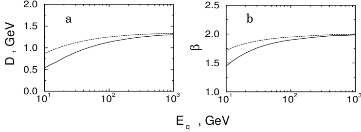
Figure 4: The parameters $D$ (a) and $\beta$ (b) for the parametrization (96) for nuclear matter. The solid lines correspond to $m_{g}=0.75$ GeV, and the dashed ones to $m_{g}=0.375$ GeV.

The $D$ and $\beta$ as function of $E_{q}$ are shown in Fig. 4 (nuclear matter) and Fig. 5 (QGP). In the region $5\mathrel{\hbox to0.0pt{\lower 4.0pt\hbox{\hskip 1.0pt$\sim$}\hss}\raise 1.0pt\hbox{$<$}}L\mathrel{\hbox to0.0pt{\lower 4.0pt\hbox{\hskip 1.0pt$\sim$}\hss}\raise 1.0pt\hbox{$<$}}10$ fm $\beta$ in (96) is by 10-20 % smaller than for $L\mathrel{\hbox to0.0pt{\lower 4.0pt\hbox{\hskip 1.0pt$\sim$}\hss}\raise 1.0pt\hbox{$<$}}5$ fm. Note that $L_{f}^{{}^{\prime}}(\mbox{max})\sim 5-10$ fm for $E_{q}\sim 10-40$ GeV in the case of nuclear matter, and $E_{q}\sim 150-600$ GeV for QGP. Then from Figs. 4, 5 one can conclude that the onset of the $L^{2}$ regime occurs at $L_{f}^{{}^{\prime}}(\mbox{max})/L\mathrel{\hbox to0.0pt{\lower 4.0pt\hbox{\hskip 1.0pt$\sim$}\hss}\raise 1.0pt\hbox{$>$}}2$. The closeness of $\beta$ to unity at $E_{q}\approx 10$ GeV for QGP agrees with a small value of $L_{f}^{{}^{\prime}}(\mbox{max})$ ($\sim 1$ fm). Our results show that the $m_{g}$-dependence of $\Delta E_{q}$ becomes weak at $E_{q}\mathrel{\hbox to0.0pt{\lower 4.0pt\hbox{\hskip 1.0pt$\sim$}\hss}\raise 1.0pt\hbox{$>$}}50$ GeV. However, it is sizeable for $E_{q}\sim 10-20$ GeV.

Our predictions for $\Delta E_{q}$ must be regarded as rough estimates with uncertainties of at least a factor of 2 in either direction. Nonetheless, rather large values of $\Delta E_{q}$ obtained for QGP indicate that the jet quenching may be an important potential probe for formation of the deconfinement phase in $AA$ collisions. A small quark energy loss obtained for nuclear matter indicates that the extraction of $\Delta E_{q}$ from experimental data on deep inelastic scattering on nuclei is a delicate problem.

4 LPM suppression in hard reactions on nuclear targets

Another important example of the LPM effect in QCD is the well-known shadowing in hard reactions on nuclear targets. For instance, nuclear shadowing in deep inelastic scattering at small values of the Bjorken variable $x_{B}=Q^{2}/2E_{\gamma^{*}}m_{p}$, here $Q^{2}$ and $E_{\gamma^{*}}$ are the photon virtuality and energy, respectively. This effect is similar to LPM suppression of pair production in QED. Calculation of the valence $q\bar{q}$ component of the shadowing correction $\Delta\sigma(\gamma^{*}A)=\sigma(\gamma^{*}A)-A\sigma(\gamma^{*}N)$ to $\gamma^{*}A$ total cross section in the limit $x_{B}\rightarrow 0$ can be performed within the frozen-size approximation [40]. The light-cone path integral formalism allows one to take into account the parton transverse motion effects, which are important for evaluation of $x_{B}$-dependence of nuclear shadowing. Nonetheless, an accurate analysis, requiring evaluation of medium effects for the higher $q\bar{q}g_{1}...g_{n}$ Fock states, is a difficult problem. However, within the Double-Leading-Log Approximation (DLLA) calculation of the leading twist contribution to $\Delta\sigma(\gamma^{*}A)$ is greatly simplified.

In the DLLA the parton light-cone variables and the transverse separations for the $q\bar{q}g_{1}...g_{n}$ state are ordered

$$x_{B}<<x_{n}<<x_{n-1}<<\ldots<<x_{1}<<x<1\,\,,$$ (97)

$$\frac{1}{Q^{2}}<<\rho^{2}<<\rho_{1}^{2}<<\ldots<<\rho_{n}^{2}\mathrel{\hbox to0.0pt{\lower 4.0pt\hbox{\hskip 1.0pt$\sim$}\hss}\raise 1.0pt\hbox{$<$}}\frac{1}{m_{g}^{2}}\,.$$ (98)

As a result, in calculating the leading twist shadowing correction, the subsystem $q\bar{q}g_{1}...g_{n-1}$ can be treated as a pointlike color-octet particle. Due to the ordering in the light-cone fractional momentum (97) the transverse motion of the center-of-mass of the $q\bar{q}g_{1}...g_{n-1}$ subsystem can be neglected, and only the motion of the softest gluon ($g_{n}$) must be taken into account. Consequently, we can write $\Delta\sigma(\gamma^{*}A)$ as

$$\Delta\sigma(\gamma^{*}A)=\Delta\sigma_{val}(\gamma^{*}A)+\Delta\sigma_{3{\bf I\!P}}(\gamma^{*}A)\,,$$ (99)

where $\Delta\sigma_{val}(\gamma^{*}A)$ corresponds to the $q\bar{q}$ Fock state of the virtual photon, while $\Delta\sigma_{3{\bf I\!P}}(\gamma^{*}A)$ gives the contribution associated with the higher $q\bar{q}g_{1}...g_{n}$ Fock states treated as a two-body octet-octet state. Both the terms on the right-hand side of (99) can be written in the form similar to Eq. (52). For $\Delta\sigma_{val}(\gamma^{*}A)$ one can obtain (to simplify notation we do not indicate spin variables)

$$\Delta\sigma_{val}(\gamma^{*}A)=-\frac{1}{2}\mbox{Re}\sum\limits_{q}\int\limits_{0}^{1}dx\int d{\mbox{{\bf b}}}\int\limits_{-\infty}^{\infty}dz_{1}n(\mbox{{\bf b}},z_{1})\int\limits_{z_{1}}^{\infty}dz_{2}n(\mbox{{\bf b}},z_{2})\int d\mbox{{\boldmath$\rho$}}\,\Psi_{\gamma^{*}}^{q*}(x,\mbox{{\boldmath$\rho$}})$$

$$\times\sigma_{2}(\rho)\Phi_{\gamma^{*}}^{q}(x,\mbox{{\boldmath$\rho$}},\mbox{{\bf b}},z_{1},z_{2})\exp\left[-\frac{i(z_{2}-z_{1})}{L_{f}^{q}}\right]\,,$$ (100)

where

$$L_{f}^{q}=\frac{2E_{\gamma^{*}}x(1-x)}{m_{q}^{2}+Q^{2}x(1-x)}\,,$$ (101)

$$\Phi_{\gamma^{*}}^{q}(x,\mbox{{\boldmath$\rho$}},\mbox{{\bf b}},z_{1},z_{2})=\int d\mbox{{\boldmath$\rho$}}^{\prime}{\cal K}_{q}(\mbox{{\boldmath$\rho$}},z_{2}|\mbox{{\boldmath$\rho$}}^{\prime},z_{1})\Psi_{\gamma^{*}}^{q}(x,\mbox{{\boldmath$\rho$}}^{\prime})\,\sigma_{2}(\rho^{\prime})\,,$$ (102)

$n(\mbox{{\bf b}},z)$ is the nuclear density, $Q^{2}$ is the photon virtuality, $\Psi_{\gamma^{*}}^{q}(x,\mbox{{\boldmath$\rho$}})$ is the light-cone wave function for transition $\gamma^{*}\rightarrow q\bar{q}$. In Eq. (102) ${\cal K}_{q}$ is the Green’s function for the Hamiltonian

$${\cal H(\mbox{{\bf b}})}=\frac{{\mbox{{\bf q}}}^{2}}{2\mu_{q\bar{q}}}+v(\mbox{{\bf b}},\mbox{{\boldmath$\rho$}},z)\,,$$ (103)

where

$$v(\mbox{{\bf b}},\mbox{{\boldmath$\rho$}},z)=-i\frac{n(\mbox{{\bf b}},z)\sigma_{2}(|\mbox{{\boldmath$\rho$}}|)}{2}\,,$$ (104)

and $\mu_{q\bar{q}}=E_{\gamma^{*}}x(1-x)$.

Using the light-cone wave functions for the $q\bar{q}g_{1}...g_{n}$ Fock states obtained in Ref. [29], we can represent $\Delta\sigma_{3{\bf I\!P}}(\gamma^{*}A)$ in the form

$$\Delta\sigma_{3{\bf I\!P}}(\gamma^{*}A)=-\frac{1}{2}\left(\frac{9}{4}\right)^{2}\mbox{Re}\int\limits_{x_{B}}^{1}dx_{g}\int d\mbox{{\bf b}}\int\limits_{-\infty}^{\infty}dz_{1}n(\mbox{{\bf b}},z_{1})\int\limits_{z_{1}}^{\infty}dz_{2}n(\mbox{{\bf b}},z_{2})\int d\mbox{{\boldmath$\rho$}}\,\lambda^{2}(x_{g},Q^{2})$$

$$\times\Psi_{\gamma^{*}}^{g*}(x_{g},\mbox{{\boldmath$\rho$}})\sigma_{2}(\rho)\Phi_{\gamma^{*}}^{g}(x_{g},\mbox{{\boldmath$\rho$}},\mbox{{\bf b}},z_{1},z_{2})\exp\left[-\frac{i(z_{2}-z_{1})}{L_{f}^{g}}\right]\,,~{}~{}~{}~{}~{}$$ (105)

where

$$L_{f}^{g}=\frac{2E_{\gamma^{*}}x_{g}}{m_{g}^{2}}\,,$$

$$\Phi_{\gamma^{*}}^{g}(x_{g},\mbox{{\boldmath$\rho$}},\mbox{{\bf b}},z_{1},z_{2})=\int d\mbox{{\boldmath$\rho$}}^{\prime}{\cal K}_{g}(\mbox{{\boldmath$\rho$}},z_{2}|\mbox{{\boldmath$\rho$}}^{\prime},z_{1})\Psi_{\gamma^{*}}^{g}(x_{g},\mbox{{\boldmath$\rho$}}^{\prime})\,\sigma_{2}(\rho^{\prime})\,.$$ (106)

The Hamiltonian for the Green’s function ${\cal K}_{g}(\mbox{{\boldmath$\rho$}},z_{2}|\mbox{{\boldmath$\rho$}}^{\prime},z_{1})$ in Eq. (106) can be obtained from Eqs. (103), (104) replacing $\mu_{q\bar{q}}$ by $\mu_{q\bar{q}g}=E_{\gamma^{*}}x_{g}$, and $\sigma_{2}$ by $\frac{9}{4}\sigma_{2}$. The factor $(9/4)^{2}$ in Eq. (105) reflects the fact that the dipole cross section for octet-octet state equals $(9/4)\sigma_{2}(\rho)$. The factor $\lambda^{2}$ in Eq. (105) coming from the internal $q\bar{q}g_{1}\ldots g_{n-1}$ states is given by

$$\lambda^{2}(x_{g},Q^{2})=\frac{4I_{0}(2\sqrt{\zeta})}{3\pi^{2}}\sum\limits_{q}\int\limits_{0}^{1}dx\int d\mbox{{\boldmath$\rho$}}\rho^{2}\alpha_{s}(\rho)|\Psi_{\gamma^{*}}^{q}(x,\mbox{{\boldmath$\rho$}})|^{2}\,,$$ (107)

where

$$\zeta=\frac{12}{\beta_{0}}\log{\left(\frac{\alpha_{s}(m_{g}^{2})}{\alpha_{s}(Q^{2})}\right)}\log{\left(\frac{1}{x_{g}}\right)}$$

is the expansion parameter of the DLLA, and $I_{0}(z)\approx\exp(z)/\sqrt{2\pi z}$ is the Bessel function. The light-cone wave function describing the softest gluon entering Eqs. (105), (106) is given by [29]

$$\Psi_{\gamma^{*}}^{g}(x_{g},\mbox{{\boldmath$\rho$}})=\frac{m_{g}}{r\sqrt{x_{g}}}\left[K_{1}(m_{g}\rho_{1})\frac{\mbox{{\bf e}}^{*}\mbox{{\boldmath$\rho$}}_{1}}{|\mbox{{\boldmath$\rho$}}_{1}|}-K_{1}(m_{g}\rho_{2})\frac{\mbox{{\bf e}}^{*}\mbox{{\boldmath$\rho$}}_{2}}{|\mbox{{\boldmath$\rho$}}_{2}|}\right]\,,$$

where e is the gluon polarization vector, and $\mbox{{\boldmath$\rho$}}_{1,2}=\mbox{{\boldmath$\rho$}}\pm\mbox{{\bf r}}/2$, $|\mbox{{\bf r}}|\sim 1/Q$. Note that, according to the derivation of Eqs. (100), (105), the perturbative component of the dipole cross section entering these equations, must be evaluated in the Born approximation.

Similar expressions can be obtained for shadowing corrections in Drell-Yan pair and heavy quark production. The results of numerical calculations of nuclear shadowing in hard reactions will be presented elsewhere.

5 Conclusion

We have discussed a new approach to the LPM effect in QED and QCD. This approach is based on the path integral representation of the light-cone wave functions. Using the unitarity we express the cross section of the radiation process $a\rightarrow bc$ in terms of the radiative correction to the transverse propagator of particle $a$. Evaluation of the cross section of transition $a\rightarrow bc$ is reduced to solving the two-dimensional Schrödinger equation with an imaginary potential proportional to the total cross section of interaction of $\bar{a}bc$ state with a medium constituent. We have demonstrated a close relationship between LPM suppression for the radiation process $a\rightarrow bc$ and the absorption correction for $\bar{a}bc$ state.

For bremsstrahlung in QED we have evaluated the LPM effect for finite-size homogeneous and structured targets. For structured targets we predict minima and maxima in the photon spectra. We have given a rigorous treatment of the Coulomb effects, which were previously treated only to a logarithmic accuracy. We have also included the inelastic process neglected in previous works. For the first time we have performed a rigorous theoretical analysis of the experimental data on the LPM effect obtained at SLAC [22]. The theoretical predictions are in very good agreement with the spectrum measured at SLAC [22] for the homogeneous gold target with $L=0.7\%X_{0}$ for 25 GeV electron beam.

For the first time we have performed a rigorous analysis of the induced gluon radiation in cold nuclear matter and in QGP within GW model [10]. For a quark incident on a nucleus we predict $\Delta E_{q}\approx 0.1E_{q}(L/10\,\mbox{fm})^{\beta}$, with $\beta$ close to unity. For a sufficiently energetic quark produced inside a medium we find the radiative energy loss $\Delta E_{q}\propto L^{2}$, where $L$ is the distance passed by the quark in the medium. It has a weak dependence on the initial quark energy. The $L^{2}$ dependence turns to $L^{1}$ as the quark energy decreases.

We have also demonstrated that the developed theory of the LPM effect can be used for an accurate evaluation of the leading twist contribution to nuclear shadowing in hard reactions on heavy nuclei.

Acknowledgements

I would like to thank R.Baier, Yu.L.Dokshitzer, P.Hoyer, J.Knoll, A.H.Mueller, N.N.Nikolaev, S.Peigne and D.Schiff for discussions. This work was partially supported by the INTAS grants 93-239ext and 96-0597.

Figures

Figure 1: The bremsstrahlung spectrum for 25 GeV electrons incident on a gold target with a thickness of $0.7\%X_{0}$. The experimental data are from Ref. [22] The full curve shows our results obtained using Eqs. (46), (51), (52). The dashed curve was obtained in the frozen-size approximation (56) The long-dashed curve shows the spectrum for the infinite medium. The Bethe-Heitler spectrum is shown by the dot-dashed curve.

Figure 2: The LPM suppression factor for 25 GeV electron incident on a homogeneous gold target as a function of the ratio $h=L/L_{f}$ and the photon momentum.

Figure 3: The LPM suppression factor for 25 GeV electron incident on a two segment gold target. The thickness of each segment is $0.35\%X_{0}$. The set of gaps is as follows: 0 (solid curve), $0.7\%X_{0}$ (dotted curve), $1.4\%X_{0}$ (dashed curve), $2.1\%X_{0}$ (long-dashed curve), $3.5\%X_{0}$ (dot-dashed curve).

Figure 5: The same as in Fig. 4 but for QGP at $T=250$ MeV.

References

• [1] L.D. Landau and I.Ya. Pomeranchuk, Dokl. Akad. Nauk SSSR 92 (1953) 535, 735.
• [2] A.B. Migdal, Phys. Rev. 103 (1956) 1811.
• [3] E.L. Feinberg and I.Ya. Pomeranchuk, Nuovo Cimento Suppl. III (1956) 602.
• [4] F.F. Ternovskii, Sov. Phys. JETP 12 (1960) 123.
• [5] V.M. Galitsky and I.I. Gurevich, Il Nuovo Cimento 32 (1964) 396.
• [6] V.E. Pafomov, Sov. Phys. JETP 20 (1965) 253.
• [7] M.L. Ter-Mikaelian, High Energy Electromagnetic Processes in Condensed Media (Wiley, NY, 1972).
• [8] M.I. Ryazanov, Sov. Phys. Usp. 17 (1975) 815, and further references therein.
• [9] A.I. Akhiezer and N.F. Shul’ga, Sov. Phys. Usp. 30 (1987) 197, and further references therein.
• [10] M. Gyulassy and X.-N. Wang, Nucl. Phys. B420 (1994) 583; X.-N. Wang, M. Gyulassy and M. Plümer, Phys. Rev. D51 (1995) 3436.
• [11] R. Baier, Yu.L. Dokshitzer, S. Peigne and D. Schiff, Phys. Lett. B345 (1995) 277.
• [12] J. Knoll and D.N. Voskresenskii, Phys. Lett. B351 (1995) 43.
• [13] N.F.Shul’ga and S.P. Fomin, JETP Lett. 63 (1996) 873.
• [14] B.G. Zakharov, JETP Lett. 63 (1996) 952.
• [15] B.G. Zakharov, JETP Lett. 64 (1996) 781.
• [16] R. Baier, Yu.L. Dokshitzer, A.H. Mueller, S. Peigne and D. Schiff, Nucl. Phys. B478 (1996) 577.
• [17] E.M. Levin, Phys. Lett. B380 (1996) 399.
• [18] R. Blankenbecler and S.D. Drell, Phys. Rev. D53 (1996) 6265.
• [19] R. Blankenbecler, Phys. Rev. D55 (1997) 190.
• [20] R. Baier, Yu.L. Dokshitzer, A.H. Mueller, S. Peigne and D. Schiff, Nucl. Phys. B483 (1997) 291; B484 (1997) 265.
• [21] B.G. Zakharov, JETP Lett. 65 (1997) 615.
• [22] P.L. Anthony, R. Becker-Szendy, P.E. Bosted et al., Phys. Rev. Lett. 75 (1995) 1949; Phys. Rev. D56 (1997) 1373.
• [23] S. Weinberg, Phys. Rev. 150 (1966) 1313.
• [24] J.B. Kogut and D.E. Soper, Phys. Rev. D1 (1970) 2901; J.M. Bjorken, J.B. Kogut and D.E. Soper, Phys. Rev. D3 (1971) 1382.
• [25] B.G. Zakharov, Sov. J. Nucl. Phys. 46 (1987) 92.
• [26] N.N. Nikolaev, G.Piller and B.G. Zakharov, JETP 81 (1995) 851.
• [27] Y.-S. Tsai, Rev. Mod. Phys. 46 (1974) 815.
• [28] E.V. Shuryak, Phys. Rep. 61 (1980) 71.
• [29] N.N. Nikolaev and B.G. Zakharov, JETP 78 (1994) 598.
• [30] N.N. Nikolaev and B.G. Zakharov, Phys. Lett. B332 (1994) 184.
• [31] F.E. Low, Phys. Rev. D12 (1975) 163; S. Nussinov, Phys. Rev. Lett. 34 (1975) 1286.
• [32] N.N. Nikolaev and B.G. Zakharov, Phys. Lett. B327 (1994) 149.
• [33] N.N. Nikolaev, B.G. Zakharov and V.R. Zoller, Phys. Lett. B328 (1994) 486.
• [34] E.V. Shuryak, Rev. Mod. Phys. 65 (1993) 1.
• [35] J. Nemchik, N.N. Nikolaev, E. Predazzi and B.G. Zakharov, Phys. Lett. B374 (1996) 199.
• [36] R.C. Moore, R.K. Clark, M. Corcoran et al., Phys. Lett. B244 (1990) 347.
• [37] E. Quack and T. Kodama, Phys. Lett. B302 (1993) 495.
• [38] S.J. Brodsky and P. Hoyer, Phys. Lett. B298 (1993) 165.
• [39] E.L. Feinberg, Sov. JETP 23 (1966) 123.
• [40] N.N. Nikolaev and B.G. Zakharov, Z. Phys. C49 (1991) 607.