Off-Forward Parton Distributions

Abstract

Recently, there have been some interesting developments involving off-forward parton distributions of the nucleon, deeply virtual Compton scattering, and hard diffractive vector-meson production. These developments are triggered by the realization that the off-forward distributions contain information about the internal spin structure of the nucleon and that diffractive electroproduction of vector mesons depends on these unconventional distributions. This paper gives a brief overview of the recent developments.

I introduction

Parton distributions were first introduced by Feynman as the phenomenological quantities describing the properties of the nucleon manifest in high-energy scattering[1]. When a nucleon travels near the speed of light, it can be viewed as consisting of a beam of non-interacting partons that are massless and collinear. Parton distributions are the densities of partons as a function of the fraction $x$ of the nucleon momentum they carry. With the advent of Quantum Chromodynamics (QCD), Feynman’s parton model, modulo logarithms, can be justified in a rigorous field theoretical approach [2]. Meanwhile, parton distributions can be expressed as the matrix elements of the bilocal light-ray operators in the ground state of the nucleon [3]. Only in the light-like gauge, $A^{+}=0$, and light-cone quantization, does their physical interpretation become apparent.

When studying the physics of parton distributions themselves, one of course can no longer regard the nucleon as consisting of free partons. Calculating these distributions requires a detailed knowledge of the nucleon wave function in quark and gluon degrees of freedom, and undoubtedly is one of the most challenging problems in nonperturbative QCD. At present, the only fundamental approach we know is the lattice QCD method [4]. On the phenomenological side, however, the unpolarized parton distributions have been extracted with good precision from various high-energy scattering data taken in the last thirty years [5, 6, 7]. The empirical parton distributions not only provide the necessary input for calculating high-energy scattering cross sections, e.g., of top-quark production, but also contain valuable information about how the nucleon is made of its constituents.

Recently, there has been much theoretical activity surrounding the so-called off-forward parton (or non-forward, off-diagonal) distributions (OFPD’s). The new distributions generalize those introduced by Feynman: They characterize certain properties of the nucleon exhibited in a class of high-energy scattering; they reflect the low-energy internal structure of the particle. However, there are also important differences between the off-forward and forward distributions. The OFPD’s in general cannot be regarded as particle densities, but rather their physical interpretation is given in terms of probability amplitude. As we shall see, they do have simple physical significance in light-cone coordinates (or the infinite momentum frame).

The most natural appearance of the OFPD’s is in non-forward high-energy processes. As far as we know, such processes were first considered by Watanabe [8] and by Bartels and M. Loewe [9]. In Ref. [8], a general virtual-photon Compton scattering off a nucleon target was studied in operator product expansion (OPE), an integral representation of the amplitude was obtained, and the off-forward matrix elements of twist-two operators were defined. The study, however, mentioned little about physical motivations and the practicality of the process; in particular, significance of the integral representation was obscure. In Ref. [9], diffractive production of $Z^{0}$ and photons was studied in perturbative QCD and the properties of the non-diagonal gluon ladder were investigated. However, no notion of an off-forward distribution of the nucleon target was apparent in the paper. Following [9], a set of off-forward evolution kernels were presented by Gribov, Levin, and Ryskin [10]. These kernels were considered as those for the scattering amplitude. The role of off-forward distributions in hard diffractive processes had remained obscured in relatively recent studies. In Ref. [11], diffractive electroproduction of $J/\psi$ was analyzed by Ryskin in the small $x$ region. The production amplitude was related to the usual Feynman gluon distribution. The off-forwardness was taken into account by a phenomenological form factor. In Refs. [12, 13, 14], Ryskin’s analysis was generalized to light vector-meson production in which the meson structure is accounted for by the leading-twist light-cone wave function.

To the author’s knowledge, one of first examples of OFPD’s was introduced by Dittes et al. [15], and was called “interpolating function.” Ironically, the main motivation for introducing such an object was not from studying any off-forward process; rather, it was considered as an example of the physical quantities whose evolution kernel interpolates between the two well-known cases: the DGLAP and ERBL evolutions [16, 17, 18]. A serious study of the OFPD in a physical process was made by D. Müller et al. [19] in which they showed that it contributes to the general two virtual-photon Compton scattering— the same process considered earlier by Watanabe. They also derived the evolution equations for the OFPD. Note that in Ref. [20] a general off-forward amplitude (or single-particle Green’s function) was introduced in studying hadron helicity flip in hard scattering. However, because the correlation of two quark fields in the object is off the light cone, it does not have a simple parton interpretation as the OFPD’s do.

The recent wave of interest in the OFPD’s was generated from two new developments. The first development is the recognition of the importance of the OFPD’s in describing the internal structure of the nucleon [21]. In studying the spin structure, it was found that the fractions of the nucleon spin carried by quarks and gluons can be determined by the form factors of the corresponding energy-momentum tensors. These form factors can be obtained from the moments of the OFPD’s which were independently introduced in [21]. In the same paper, deeply virtual Compton scattering (DVCS) was proposed as a practical means to measure the OFPD’s. In DVCS, a highly virtual photon scatters off a quark in a nucleon target, which then emits a real photon and returns to form a recoil nucleon. Although the two-photon process studied earlier by Watanabe and Müller et al. contains DVCS as its special kinematic limit, the latter has important experimental advantages and a special theoretical status. Indeed, DVCS is more delicate to treat theoretically because of an extra light-like vector among the external momenta.

The second development is the realization that hard diffractive electroproduction of vector mesons requires the use of OFPD’s [22, 21]. The first serious studies in this direction were made by Radyushkin [23], Hoodbhoy [24], and Collins et al. [25]. In Ref. [23], an off-forward gluon distribution - most important in the low $x$ region - was introduced and used to calculate vector meson production in deep-inelastic electron scattering. The result is free of the assumptions made in Ref. [12] about the dominance of the absorptive contribution and the use of the forward gluon distribution. Hoodbhoy [24] used the off-forward gluon distribution to calculate heavy quarkonium production investigated earlier by Ryskin [11]. He obtained a similar result as Radyushkin’s. In a comprehensive paper, Collins, Frankfurt, and Strikman showed that a factorization theorem exists for general hard diffractive meson production in deep-inelastic scattering [25]. The factorization theorem explicitly involves the OFPD’s.

Recently, many works have been produced in studying off-forward parton distributions, deeply virtual Compton scattering, and diffractive vector meson production. It is the goal of this paper to review these interesting developments. In section II, off-forward distributions are introduced from different perspectives and various definitions in the literature are compared. In section III, we make a digression to discuss the spin structure of the nucleon. The role of the OFPD’s in this interesting subject is exposed. In section IV, we summarize our present knowledge about the OFPD’s at hadron mass scales and their evolution to high-energy scales. In section V, we consider processes in which the OFPD’s may actually be measured: deeply virtual Compton scattering and hard diffractive vector-meson production. Section VI contains the summary and outlook.

II Definitions and Interpretations

Since the off-forward distributions contain rich information about the nucleon structure, it is instructive to examine their definitions and interpretations from different angles. In this section, we will first introduce the off-forward distributions from the form factors of twist-two operators and then we explore their significance in light-cone coordinates. Finally we compare the OFPD’s with other equivalent definitions in the literature.

A Elastic Form Factors of Twist-Two Operators

From the point view of the low-energy nucleon structure, it is perhaps most interesting to consider the off-forward distributions as the generating functions for the form factors of the so-called twist-two operators. Recall that the matrix elements of the electromagnetic current in the equal momentum states are entirely determined by symmetry, whereas those in the unequal momentum states define the (Dirac and Pauli) form factors which contain such interesting information as charge radius and magnetic moment of the nucleon. The following tower of twist-two operators represents a generalization of the electromagnetic current

$${\cal O}^{\mu_{1}\cdots\mu_{n}}_{q}=\overline{\psi}_{q}i\stackrel{{\scriptstyle\leftrightarrow}}{{\cal D}}^{(\mu_{1}}\cdots i\stackrel{{\scriptstyle\leftrightarrow}}{{\cal D}}^{\mu_{n-1}}\gamma^{\mu_{n})}\psi_{q}\ ,$$ (1)

where all indices are symmetrized and traceless (indicated by $(\cdots)$) and $\stackrel{{\scriptstyle\leftrightarrow}}{{\cal D}}=(\stackrel{{\scriptstyle\rightarrow}}{{\cal D}}-\stackrel{{\scriptstyle\leftarrow}}{{\cal D}})/2.$ Technically, these operators transform like $(n/2,n/2)$ under Lorentz transformations. Our interest in such operators is not accidental. They appear, for instance, in the operator production expansion of the two electromangetic currents in deep-inelastic scattering [26]. Thus although these generalized currents do not couple directly to any known fundamental interactions, they can nonetheless be studied indirectly in hard scattering processes.

Since the operators for $n>1$ are not related to any symmetry in the QCD lagrangian, their matrix elements between the equal momentum states,

$$\langle P|{\cal O}^{\mu_{1}\cdots\mu_{n}}_{q}|P\rangle=2a_{n}(\mu)P^{(\mu_{1}}\cdots P^{\mu_{n})}\ ,$$ (2)

contain valuable dynamical information about the internal structure of the nucleon. In this paper, we use the covariant normalization $\langle P|P\rangle=2E(2\pi)^{3}\delta^{3}(0)$ for the nucleon state. The $\mu$ dependence of the above matrix elements signifies the dependence on renormalization scale and scheme [26]. The quark distribution $q(x,\mu)$ introduced by Feynman has a simple connection to the above matrix elements:

$$\int^{1}_{-1}dxx^{n-1}q(x,\mu)=a_{n}(\mu)\ ,$$ (3)

where $q(x,\mu)$ is chosen to have support in $(-1,1)$. For $x>0$, $q(x,\mu)$ is the just density of quarks which carry the $x$ fraction of the parent nucleon momentum. The density of antiquarks is customarily denoted as $\bar{q}(x,\mu)$, which in the above notation is $-q(-x,\mu)$ [2].

Just like the form factors of the electromagnetic current, additional information about nucleon structure can be found in the form factors of the twist-two operators when the matrix elements are taken between the states of unequal momenta. Using Lorentz symmetry and parity and time reversal invariance, one can write down all possible form factors of the spin-$n$ operator

$$\langle P^{\prime}|O^{\mu_{1}\cdots\mu_{n}}_{q}|P\rangle = {\overline{U}}(P^{\prime})\gamma^{(\mu_{1}}U(P)\sum_{i=0}^{[{n-1\over 2}]}A_{qn,2i}(t)\Delta^{\mu_{2}}\cdots\Delta^{\mu_{2i+1}}\overline{P}^{\mu_{2i+2}}\cdots\overline{P}^{\mu_{n})}$$ (6)

$$+~{}{\overline{U}}(P^{\prime}){\sigma^{(\mu_{1}\alpha}i\Delta_{\alpha}\over 2M}U(P)\sum_{i=0}^{[{n-1\over 2}]}B_{qn,2i}(t)\Delta^{\mu_{2}}\cdots\Delta^{\mu_{2i+1}}\overline{P}^{\mu_{2i+2}}\cdots\overline{P}^{\mu_{n})}$$

$$+~{}C_{qn}(t)~{}{\rm Mod}(n+1,2)~{}{1\over M}\bar{U}(P^{\prime})U(P)\Delta^{(\mu_{1}}\cdots\Delta^{\mu_{n})}\ ,$$

where ${\overline{U}}(P^{\prime})$ and $U(P)$ are the Dirac spinors and $Mod(n+1,2)$ is 1 when $n$ even, 0 when $n$ odd. The four-momentum transfer is denoted by $\Delta=P^{\prime}-P$ and its invariant by $t=\Delta^{2}$. The average nucleon momentum $\overline{P}=(P^{\prime}+P)/2$ is also a useful variable. For $n\geq 1$, even or odd, there are $n+1$ form factors. $C_{qn}(t)$ is present only when $n$ is even.

As the forward matrix elements $a_{n}$, the above form factors can be used to define a new type of parton distributions—off-forward distributions. To accomplish this, we introduce a light-like vector $n^{\mu}$, which is conjugate to $\overline{P}$ in the sense that $\bar{P}\cdot n=1$. Write $\overline{P}=p+(\overline{M}^{2}/2)n$, where $\overline{M}^{2}=M^{2}-t/4$ and $p$ is another light-like vector. Contracting both sides of Eq. (6) with $n_{\mu_{1}}\cdots n_{\mu_{n}}$, we have

$$n_{\mu_{1}}\cdots n_{\mu_{n}}\langle P^{\prime}|O^{\mu_{1}\cdots\mu_{n}}_{q}|P\rangle={\overline{U}}(P^{\prime})\not\!nU(P)H_{qn}(\xi,t)+{\overline{U}}(P^{\prime}){\sigma^{\mu\alpha}n_{\mu}i\Delta_{\alpha}\over 2M}U(P)E_{qn}(\xi,t)\ ,$$ (7)

where

$$H_{qn}(\xi,t) = \sum_{i=0}^{[{n-1\over 2}]}A_{qn,2i}(t)(-2\xi)^{2i}+{\rm Mod}(n+1,2)~{}C_{qn}(t)(-2\xi)^{n}\ ,$$ (8)

$$E_{qn}(\xi,t) = \sum_{i=0}^{[{n-1\over 2}]}B_{qn,2i}(t)(-2\xi)^{2i}-{\rm Mod}(n+1,2)~{}C_{qn}(t)(-2\xi)^{n}\ .$$ (9)

Here we have defined a new variable $\xi=-n\cdot\Delta/2$. Clearly, the $\xi$ dependence of $H_{qn}$ and $E_{qn}$ helps to distinguish among the different form factors of the same operator. Now one can introduce the off-forward parton distributions (OFPD’s) $H(x,\xi,t)$ and $E(x,\xi,t)$ through their moments

$$\int^{1}_{-1}dxx^{n-1}E_{q}(x,\xi,t) = E_{qn}(\xi,t)\ ,$$ (10)

$$\int^{1}_{-1}dxx^{n-1}H_{q}(x,\xi,t) = H_{qn}(\xi,t)\ .$$ (11)

Since all form factors are real, the new distributions are consequently real. Moreover, because of time-reversal and hermiticity, they are even functions of $\xi$. For simplicity, we have not shown here the renormalization scale dependence. Frequently we will also omit the $t$ dependence.

The new distributions are more complicated than the Feynman parton distributions because of their dependence on the momentum transfer $\Delta$. As such, the OFPD’s contain two more scalar variables besides the Feynman variable $x$. The variable $t$ is the usual $t$-channel invariant which is always present in a form factor. The $\xi$ variable is a natural product of marrying the concepts of the Feynman distribution and form factor: The former requires the presence of a prefered momentum $p^{\mu}$ along which the partons are predominantly moving and the latter requires a four-momentum transfer $\Delta$; $\xi$ is just a scalar product of the two momenta. Some insights about the dependence of the OFPD’s on these two extra variables will be offered later in Section IV.A.

In QCD, there are five additional towers of twist-two operators besides that in Eq. (1):

$$\tilde{\cal O}^{\mu_{1}\cdots\mu_{n}}_{q} = \overline{\psi}_{q}i\stackrel{{\scriptstyle\leftrightarrow}}{{\cal D}}^{(\mu_{1}}\cdots i\stackrel{{\scriptstyle\leftrightarrow}}{{\cal D}}^{\mu_{n-1}}\gamma^{\mu_{n})}\gamma_{5}\psi_{q}\ ,$$ (12)

$${\cal O}^{\mu_{1}\cdots\mu_{n}\alpha}_{qT} = \overline{\psi}_{q}i\stackrel{{\scriptstyle\leftrightarrow}}{{\cal D}}^{(\mu_{1}}\cdots i\stackrel{{\scriptstyle\leftrightarrow}}{{\cal D}}^{\mu_{n-1}}\sigma^{\mu_{n})\alpha}\psi_{q}\ ,$$ (13)

$${\cal O}^{\mu_{1}\cdots\mu_{n}}_{g} = F^{(\mu_{1}\alpha}i\stackrel{{\scriptstyle\leftrightarrow}}{{\cal D}}^{\mu_{2}}\cdots i\stackrel{{\scriptstyle\leftrightarrow}}{{\cal D}}^{\mu_{n-1}}F_{\alpha}^{~{}\mu_{n})}\ ,$$ (14)

$$\tilde{\cal O}^{\mu_{1}\cdots\mu_{n}}_{g} = F^{(\mu_{1}\alpha}i\stackrel{{\scriptstyle\leftrightarrow}}{{\cal D}}^{\mu_{2}}\cdots i\stackrel{{\scriptstyle\leftrightarrow}}{{\cal D}}^{\mu_{n-1}}i\tilde{F}_{\alpha}^{~{}\mu_{n})}\ ,$$ (15)

$${\cal O}^{\mu_{1}\cdots\mu_{n}\alpha\beta}_{gT} = F^{(\mu_{1}\alpha}i\stackrel{{\scriptstyle\leftrightarrow}}{{\cal D}}^{\mu_{2}}\cdots i\stackrel{{\scriptstyle\leftrightarrow}}{{\cal D}}^{\mu_{n-1}}F^{\mu_{n})\beta}\ .$$ (16)

The corresponding off-forward distributions can be labelled by $\Big{(}\tilde{H}_{q}(x,\xi)$, $\tilde{E}_{q}(x,\xi)\Big{)}$, $\Big{(}H_{Tq}(x,\xi)$, $E_{Tq}(x,\xi)\Big{)}$, $\Big{(}H_{g}(x,\xi)$, $E_{g}(x,\xi)\Big{)}$, $\Big{(}\tilde{H}_{g}(x,\xi)$, $\tilde{E}_{g}(x,\xi)\Big{)}$, and $\Big{(}H_{Tg}(x,\xi)$, $E_{Tg}(x,\xi)\Big{)}$, respectively.

B OFPD’s in Light-Cone Coordinates and Gauge

The physical significance of parton distributions in high-energy processes is apparent only in light-cone coordinates and light-cone gauge. To see this, we sum up all the local twist-two operators into a light-cone bilocal operator and express the parton distributions in terms of the latter,

$$F_{q}(x,\xi,t) ={1\over 2}\int{d\lambda\over 2\pi}e^{i\lambda x}\left\langle P^{\prime}\left|\overline{\psi}_{q}\left(-{\lambda\over 2}n\right)\not\!n{\cal P}e^{-ig\int^{-\lambda/2}_{\lambda/2}d\alpha~{}n\cdot A(\alpha n)}\psi_{q}\left({\lambda\over 2}n\right)\right|P\right\rangle$$ (18)

$$=H_{q}(x,\xi,t)~{}{1\over 2}\overline{U}(P^{\prime})\not\!nU(P)+E_{q}(x,\xi,t)~{}{1\over 2}\overline{U}(P^{\prime}){i\sigma^{\mu\nu}n_{\mu}\Delta_{\nu}\over 2M}U(P)\ .$$

The light-cone bilocal operator (or light-ray operator) arises frequently in hard scattering processes in which partons propagate along the light-cone. In fact, the Taylor-expansion of this operator along the light-cone leads us immediately to the twist-two operators considered in the last subsection. The parton distributions are most naturally defined in terms of the matrix elements of the bilocal operator. In this context, the Feynman $x$ is just the Fourier variable of the light-cone distance. The Lorentz structures in the second line in the above equation are independent and complete.

In ordinary coodinates, the correlation of two quark fields in the light-ray operator is in both space and time. As such, the physical interpretation is quite complicated. However, in light-cone coordinates, the physical content of the bilocal operator becomes transparent. To see this, let us recall that the light-cone coordinates are defined as,

$$x^{\pm} = {1\over\sqrt{2}}(x^{0}\pm x^{3})\ ,$$ (19)

$$x_{\perp} = (x^{1},x^{2})\ .$$ (20)

In this new system of coordinates, the role of time is played by $x^{+}$. In the same fashion, introduce the light-cone Dirac matrices $\gamma^{\pm}$ and the projection operators, $P_{\pm}={1\over 2}\gamma^{\mp}\gamma^{\pm}$. A Dirac field $\psi$ can be decomposed into a sum of $\psi_{+}=P_{+}\psi$, the independent degrees of freedom (“good”), and $\psi_{-}=P_{-}\psi$, the dependent degrees of freedom (“bad”). In light-cone quantization, the independent components of the Dirac field obey the following commutation relation [27]

$$\left[\psi_{+\alpha}(x),\psi_{+\beta}^{\dagger}(y)\right]_{+}|_{x^{+}=y^{+}}={1\over\sqrt{2}}P_{+\alpha\beta}\delta(x^{-}-y^{-})\delta^{2}(x_{\perp}-y_{\perp})\ ,$$ (21)

where $[~{}]_{+}$ denotes anticommutation. The above relation can be solved by a Fourier expansion

$$\psi_{+}(x^{-},x_{\perp}) = \int{dk^{+}d^{2}\vec{k}_{\perp}\over 2k^{+}(2\pi)^{3}}\theta(k^{+})\sum_{\lambda=\pm}\left(b_{\lambda}(k^{+},\vec{k}_{\perp})u_{\lambda}(k)e^{-i(x^{-}k^{+}-\vec{x}_{\perp}\cdot\vec{k}_{\perp})}\right.$$ (23)

$$\left.+~{}d_{\lambda}^{\dagger}(k^{+},\vec{k}_{\perp})v_{\lambda}(k)e^{i(x^{-}k^{+}-\vec{x}_{\perp}\cdot\vec{k}_{\perp})}\right)\ ,$$

and similarly for $\overline{\psi}_{+}$. The quark (antiquark) creation and annihilation operators, $b_{\lambda k}^{\dagger}$ ($d_{\lambda k}^{\dagger})$ and $b_{\lambda k}$ ($d_{\lambda k})$, obey the commutation relation

$$\left[b_{\lambda}(k^{+},\vec{k}_{\perp}),b^{\dagger}_{\lambda^{\prime}}({k^{\prime}}^{+},\vec{k^{\prime}}_{\perp})\right]_{+} = 2k^{+}\delta_{\lambda\lambda^{\prime}}(2\pi)^{3}\delta(k^{+}-k^{\prime+})\delta^{2}(k_{\perp}-k_{\perp}^{\prime})\ ,$$ (24)

$$\left(~{}\left[d_{\lambda}(k^{+},\vec{k}_{\perp}),d^{\dagger}_{\lambda^{\prime}}({k^{\prime}}^{+},\vec{k^{\prime}}_{\perp})\right]_{+}\right. = \left.2k^{+}\delta_{\lambda\lambda^{\prime}}(2\pi)^{3}\delta(k^{+}-k^{\prime+})\delta^{2}(k_{\perp}-k_{\perp}^{\prime})\ .\right)$$ (25)

In the presence of a gauge field, the above is unchanged if the light-cone gauge, $A^{+}=0$, is chosen. The same gauge choice eliminates the gauge link in the light-ray operator.

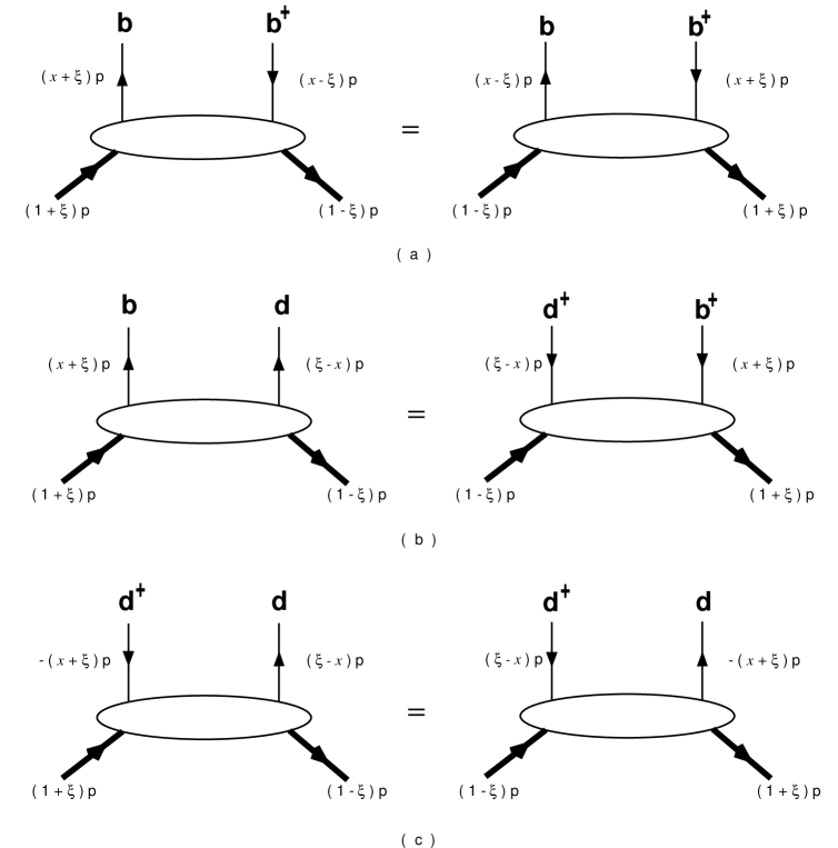
FIG. 1.: Diagrams showing $\xi$ symmetry of the off-forward parton distributions: a) $x>\xi$; b) $\xi>x>-\xi$; c) $x<-\xi$.

Now we can look at the physical content of the off-forward distributions in the light-cone coordinates and gauge. Since they are even in $\xi$, we first restrict ourselves to $\xi>0$. Substituting the light-cone Fock expansion into Eq. (18), we have

$$F_{q}(x,\xi) = {1\over 2p^{+}V}\int{d^{2}k_{\perp}\over 2\sqrt{|x^{2}-\xi^{2}|}(2\pi)^{3}}\sum_{\lambda}$$ (26)

$$\times \left\{\begin{array}[]{ll}\left\langle P^{\prime}\left|b^{\dagger}_{\lambda}\left((x-\xi)p^{+},\vec{k}_{\perp}+\vec{\Delta}_{\perp}\right)b_{\lambda}\left((x+\xi)p^{+},\vec{k}_{\perp}\right)\right|P\right\rangle\ ,&{\rm for}~{}x>\xi\\ \left\langle P^{\prime}\left|d_{\lambda}\left((-x+\xi)p^{+},-\vec{k}_{\perp}-\vec{\Delta}_{\perp}\right)b_{-\lambda}\left((x+\xi)p^{+},\vec{k}_{\perp}\right)\right|P\right\rangle\ ,&{\rm for}~{}\xi>x>-\xi\\ -\left\langle P^{\prime}\left|d^{\dagger}_{\lambda}\left((-x-\xi)p^{+},\vec{k}_{\perp}+\vec{\Delta}_{\perp}\right)d_{\lambda}\left((-x+\xi)p^{+},\vec{k}_{\perp}\right)\right|P\right\rangle\ ,&{\rm for}~{}x<-\xi\end{array}\right.$$ (30)

where $V$ is a volume factor. The distribution has different physical interpretations in the three different regions. In the region $x>\xi$, it is the amplitude for taking a quark of momentum $k$ out of the nucleon, changing its momentum to $k+\Delta$, and inserting it back to form a recoiled nucleon. In the region $\xi>x>-\xi$, it is the amplitude for taking out a quark and antiquark pair with momentum $-\Delta$. Finally, in the region $x<-\xi$, we have the same situation as in the first, except the quark is replaced by an antiquark. The first and third regions are similar to those present in the ordinary parton distributions and hence will be called the DGLAP region. The middle region is similar to that in a meson amplitude and hence will be called the ERBL region.

The $\xi$ symmetry is an important property of the OFPD’s. To illustrate the parton content of this symmetry, one can work out the equivalent of Eq. (30) by assuming $\xi$ is negative. The result is best shown in Fig. 1, where the quark and antiquark creations and annihilations are indicated explicitly.

From Eq. (30), the off-forward distribution is very much like a quark-nucleon scattering amplitude. Use ${\cal A}_{Hh,H^{\prime}h^{\prime}}$ to label the helicity amplitudes, where $H,H^{\prime}$ are the helicities of the initial and final nucleons and $h,h^{\prime}$ are those of the created and annihilated quarks. Time-reversal and parity invariance provide the constraints ${\cal A}_{Hh,H^{\prime}h^{\prime}}={\cal A}_{H^{\prime}h^{\prime},Hh}$ and ${\cal A}_{Hh,H^{\prime}h^{\prime}}={\cal A}_{-H-h,-H^{\prime}-h^{\prime}}$. Therefore, there are total of six independent helicity amplitudes which imply four additional twist-two off-forward distributions [28]

$$\tilde{F}_{q}(x,\xi) ={1\over 2}\int{d\lambda\over 2\pi}e^{i\lambda x}\left\langle P^{\prime}\left|\overline{\psi}_{q}\left(-{\lambda\over 2}n\right)\not\!n\gamma_{5}{\cal P}e^{-ig\int^{-\lambda/2}_{\lambda/2}d\alpha~{}n\cdot A(\alpha n)}\psi_{q}\left({\lambda\over 2}n\right)\right|P\right\rangle$$ (32)

$$=\tilde{H}_{q}(x,\xi,t)~{}{1\over 2}\overline{U}(P^{\prime})\not\!n\gamma_{5}U(P)+\tilde{E}_{q}(x,\xi,t)~{}{1\over 2}\overline{U}(P^{\prime}){\gamma_{5}\Delta\cdot n\over 2M}U(P)\ .$$

$$F_{Tq}(x,\xi) ={1\over 2}\int{d\lambda\over 2\pi}e^{i\lambda x}\left\langle P^{\prime}\left|\overline{\psi}_{q}\left(-{\lambda\over 2}n\right)n_{\mu}\sigma^{\mu\perp}{\cal P}e^{-ig\int^{-\lambda/2}_{\lambda/2}d\alpha~{}n\cdot A(\alpha n)}\psi_{q}\left({\lambda\over 2}n\right)\right|P\right\rangle$$ (34)

$$=H_{Tq}(x,\xi)~{}{1\over 2}\overline{U}(P^{\prime})n_{\mu}\sigma^{\mu\perp}U(P)+E_{Tq}(x,\xi)~{}{1\over 2}\overline{U}(P^{\prime}){n_{\mu}\gamma^{[\mu}i\Delta^{\perp]}\over M}U(P)\ .$$

Their parton interpretation is similar to that of $F_{q}(x,\xi)$, except that for $\tilde{F}_{q}(x,\xi)$ there is a sign depending on the quark helicity and for $F_{Tq}(x,\xi)$ there is a quark helicity flip [29].

Off-forward gluon distributions can be introduced in the similar fashion. Consider first the gluon-nucleon helicity amplitudes. Symmetries limit the number of independent ones to six, and hence there are six leading-twist gluon distributions. Here we quote only the helicity-independent ones:

$$F_{G}(x,\xi) = {1\over 2x}\int{d\lambda\over 2\pi}e^{i\lambda x}\left\langle P^{\prime}\left|F^{\mu\alpha}\left(-{\lambda\over 2}n\right)F_{\alpha}^{~{}\nu}\left({\lambda\over 2}n\right)\right|P\right\rangle n_{\mu}n_{\nu}$$ (35)

$$= H_{g}(x,\xi)~{}{1\over 2}\overline{U}(P^{\prime})\not\!nU(P)+E_{g}(x,\xi)~{}{1\over 2}\overline{U}(P^{\prime}){i\sigma^{\mu\nu}n_{\mu}\Delta_{\nu}\over 2M}U(P)\ ,$$ (36)

where the gauge link is not shown. Because of the Bose symmetry, $F_{G}(x,\xi)=-F_{G}(-x,\xi)$. The interested reader can find the other twist-two gluon distributions in [28].

In light-front coordinates, only $A_{\perp}$ are the independent degrees of freedom. They obey the commutation relation [27]

$$[A_{i}(x),A_{j}(y)]|_{x^{+}=y^{+}}={1\over 2}\delta_{ij}\delta^{2}(x_{\perp}-y_{\perp})\epsilon(x^{-}-y^{-})$$ (37)

where $\epsilon(a-b)=\theta(a-b)-\theta(b-a)$. The commutation relation can be solved by the following expansion

$$A_{i}(x^{-},x_{\perp}) = \int{dk^{+}d^{2}\vec{k}_{\perp}\over 2k^{+}(2\pi)^{3}}\theta(k^{+})\sum_{\lambda=\pm}\left(a_{\lambda}(k^{+},\vec{k}_{\perp})\epsilon_{i}(\lambda,k)e^{-i(x^{-}k^{+}-\vec{x_{\perp}}\cdot\vec{k_{\perp}})}\right.$$ (39)

$$~{}~{}~{}~{}~{}\left.+a_{\lambda}^{\dagger}(k^{+},\vec{k}_{\perp})\epsilon^{*}_{i}(\lambda,k)e^{i(x^{-}k^{+}-\vec{x_{\perp}}\cdot\vec{k_{\perp}})}\right)\ ,$$

where $a^{\dagger}_{\lambda}(k)$ and $a_{\lambda}(k)$ are the gluon creation and annihilation operators. Using this expansion, the physical content of the gluon distributions can be worked out immediately

$$F_{G}(x,\xi) = {1\over 4p^{+}V}\int{d^{2}k_{\perp}\over 2\sqrt{|x^{2}-\xi^{2}|}(2\pi)^{3}}\sum_{\lambda}$$ (40)

$$\times \left\{\begin{array}[]{ll}\left\langle P^{\prime}\left|a^{\dagger}_{\lambda}\left((x-\xi)p^{+},\vec{k}_{\perp}+\vec{\Delta}_{\perp}\right)a_{\lambda}\left((x+\xi)p^{+},\vec{k}_{\perp}\right)\right|P\right\rangle\ ,&{\rm for}~{}x>\xi\\ \left\langle P^{\prime}\left|a_{\lambda}\left((-x+\xi)p^{+},-\vec{k}_{\perp}-\vec{\Delta}_{\perp}\right)a_{-\lambda}\left((x+\xi)p^{+},\vec{k}_{\perp}\right)\right|P\right\rangle\ ,&{\rm for}~{}\xi>x>0\end{array}\right.$$ (43)

In the region $x>\xi$, it is the amplitude for taking a gluon of momentum $k$ out of the nucleon, changing its momentum to $k+\Delta$, and inserting it back to form a recoiled nucleon. In the region $\xi>x>0$, it is the amplitude for taking out a gluon pair with momentum $-\Delta$.

In an actual calculation of the distributions, the vacuum subtraction in matrix elements is always implied. As such, it is convenient to insert a $T$ product between the two fields at light-cone separations. The difference between a $T$ product and an ordinary product is just a constant

$$T\psi^{\dagger}_{+}(0)\psi_{+}(\lambda n)=\psi^{\dagger}_{+}(0)\psi_{+}(\lambda n)-\theta(\lambda n^{0})\left[\psi^{\dagger}_{+}(0),\psi_{+}(\lambda n)\right]_{+}\ .$$ (44)

The constant does not contribute to any physical matrix element. Therefore, a light-cone $T$ product contains only dispersive contributions.

C Other Notations and Definitions

The notion of OFPD’s we discussed above are essentially that of Refs. [19] and [21]. The variables $x$ and $\xi$ here are the same as the variables $t$ and $\tau$ in [19]. Other names (non-forward distributions, off-diagonal distributions, double distributions) and notations exist in the literature.

Radyushkin introduced the non-forward distributions ${\cal F}_{\zeta}(X)$ in Refs. [23, 30]. To see their relationship to the OFPD’s, one can write Eq. (18) for an arbitrary light-like $n$

$$~{}~{}\int{d\lambda\over 2\pi}e^{i\lambda k\cdot n}\left\langle P^{\prime}\left|\overline{\psi}_{q}\left(-{\lambda\over 2}n\right)\not\!n{\cal P}e^{-ig\int^{-\lambda/2}_{\lambda/2}d\alpha~{}n\cdot A(\alpha n)}\psi_{q}\left({\lambda\over 2}n\right)\right|P\right\rangle$$ (45)

$$=H_{q}\left({n\cdot k\over n\cdot\overline{P}},-{n\cdot\Delta\over 2n\cdot\overline{P}}\right){1\over n\cdot\overline{P}}\overline{U}(P^{\prime})\not\!nU(P)$$ (46)

$$+~{}E_{q}\left({n\cdot k\over n\cdot\overline{P}},-{n\cdot\Delta\over 2n\cdot\overline{P}}\right){1\over n\cdot\overline{P}}\overline{U}(P^{\prime}){i\sigma^{\mu\nu}n_{\mu}\Delta_{\nu}\over 2M}U(P)\ .$$ (47)

One can also shift the argument of the string operator using Heisenberg’s equations of motion. Now if one chooses

$$n\cdot P=1,~{}~{}X=k\cdot n,~{}~{}\zeta=-\Delta\cdot n\ ,$$ (48)

the variables are related according to

$$x = {X-\zeta/2\over 1-\zeta/2},~{}~{}~{}~{}\xi={\zeta/2\over 1-\zeta/2}\ ;$$ (49)

$$X = {x+\xi\over 1+\xi},~{}~{}~{}~{}\zeta={2\xi\over 1+\xi}\ .$$ (50)

The matrix element of the string operator becomes

$$\int{d\lambda\over 2\pi}e^{i\lambda X}\left\langle P\left|\overline{\psi}_{q}(0)\not\!n{\cal P}e^{-ig\int^{0}_{\lambda/2}d\alpha~{}n\cdot A(\alpha n)}\psi_{q}\left(\lambda n\right)\right|P\right\rangle=F_{q}(x,\xi,t)$$ (51)

$$=(1+\xi)H_{q}(x,\xi)\overline{U}(P^{\prime})\not\!nU(P)+~{}(1+\xi)E_{q}(x,\xi)\overline{U}(P^{\prime}){i\sigma^{\mu\nu}n_{\mu}\Delta_{\nu}\over 2M}U(P)\ .$$ (52)

Compared with Eqs. (9.1) and (9.2) in Ref. [30], we have

$$(1+\xi)H_{q}(x,\xi)={\cal F}_{\zeta}^{q}(X)\theta(0<X<1)-{\cal F}_{\zeta}^{\bar{q}}(\zeta-X)\theta(-1+\zeta\leq X\leq\zeta)\ .$$ (53)

The advantages of $H(x,\xi)$ over ${\cal F}_{\zeta}(X)$ are: 1) it treats the initial and final nucleon symmetrically and thus $\xi$ symmetry is obvious; 2) it has a simple connection with local hermitian operators. However, the $X$ variable in ${\cal F}_{\zeta}(X)$ has the advantage of measuring one of the initial parton momenta according to the longitudinal momentum of the initial nucleon, analogous to the forward case.

Collins et al. introduced the off-diagonal distributions $f(x_{1},x_{2},t)$ [25]. They also chose the $n$ vector conjugate to the initial state momentum. The relations of their variables to ours are,

$$x_{1} = {x+\xi\over 1+\xi},~{}~{}~{}~{}x_{2}={x-\xi\over 1+\xi}\ ;$$ (54)

$$x = {(x_{1}+x_{2})/2\over 1-(x_{1}-x_{2})/2},~{}~{}\xi={(x_{1}-x_{2})/2\over 1-(x_{1}-x_{2})/2}\ .$$ (55)

Here $x_{1}$ is the same as Radyuskin’s $X$. The off-diagonal distributions are related to the OFPD’s by

$$f_{q/p}(x_{1},x_{2})=F_{q}(x,\xi).$$ (56)

On the other hand, for gluons, one has

$$x_{1}x_{2}f_{g/p}(x_{1},x_{2},t)=2xF_{g}(x,\xi)\ .$$ (57)

Again, the $\xi$ symmetry is not obvious in these off-diagonal distributions.

Radyushkin also introduced what he called double distributions $F(x,y)$, where $x$ and $y$ are the fractions of the initial nucleon momentum $P$ and the momentum transfer $\Delta$ carried by the active parton [31]. It is interesting from the point of view of parametrizing the momentum flow out of a hadron vertex in a $\xi$-independent way. However, the physics of a double distribution is equivalent to that of the corresponding off-forward distribution.

III OFPD’s and The Spin Structure of the Nucleon

One of the principal motivations for studying off-forward distributions is that they provide a new class of observables for the internal structure of the nucleon. We believe that the physics of strong interactions is described by the fundamental theory–quantum chromodynamics (QCD). However, QCD in the low-energy region is strongly interacting and highly relativistic, involving an infinite number of degrees of freedom. No theory of this type has ever been solved before with a clear physical insight. The only available tool now for solving QCD bound states is lattice QCD [4]. At this stage, the approach has not yet been developed to a degree of sophistication so that one can reliably calculate fundamental observables with respectable precisions. Therefore, any experimental information on the structure of the nucleon is valuable in helping to understand how nature constructed this particle of extreme importance to our existence.

Since Gell-Mann and Zweig’s quark model, many nucleon models have been proposed to correlate the experimental data from low and high energy probes. Although these models are not precisely QCD, they have been quite successful phenomenologically. However, the ultimate question confronting models is how the degrees of freedom used in them are related to those in QCD. This question is of high importance because experimental probes do not couple to model degrees of freedom. In practice, simple assumptions have been used in comparing model predictions and data, e.g., the constituent quarks are identified as QCD quarks at low-energy scales although a precise notation of the latter is unclear. These assumptions have been seriously challenged in 1987 when the European Muon Collaboration (EMC) measured, with an unprecedented precision, the proton’s spin-dependent structure function $G_{1}(Q^{2},\nu)$ in polarized deep-inelastic scattering. Combining their data with the hyperon beta decay rates, augmented with the assumption of the flavor SU(3) symmetry, EMC extracted the fraction of the nucleon spin carried in the spin of quarks:

$$\Delta\Sigma\left(\overline{Q}^{2}\!=\!10{\rm GeV}^{2}\right)=0.12\pm 0.17\ .$$ (58)

This result is in flat contradiction with the cherished quark model prediction $\Delta\Sigma=1$. This so-called “spin crisis” has touched off an explosive activity in both theoretical and experimental communities. After ten more years of careful experimental studies, the original EMC result has essentially been confirmed, although the small $x$ contribution to $\Delta\Sigma$ remains largely uncertain. A recent global analysis of the data can be found, for instance, in Ref. [32].

Many theoretical “solutions” to the “spin crisis” have been proposed in the literature. Apart from doubts about the experimental data and the interpretation of them, there have been serious attempts in explaining the EMC result from the fundamental theory. For instance, lattice QCD calculations have produced numbers close to the EMC result [33, 34, 35], although the systematic effects of quenched approximation, finite lattice sizes, and large quark masses remain uncertain. Despite these, more fundamental approaches have not yet offered a complete picture about the spin structure of the nucleon. As to the naive quark model prediction, the key question is what has been alluded to abovel: namely, whether the quark model result can be directly compared with the experimental data, or whether the constituent quarks are the same as the QCD quarks probed in high-energy scattering. No convincing argument has been offered towards a positive answer.

More recently, progress has been made in attempting to understand how QCD builds up the nucleon spin. The progress potentially has an important impact on other theoretical studies, and ultimately on our basic knowledge of the internal structure of the nucleon. On the one hand, it suggests a thorough examination of the spin structure in a fundamental way. On the other hand, they called for understanding the role of the gluon degrees of freedom in model building. As it turns out, a key element in unraveling the nucleon spin is the off-forward parton distributions.

The history began with identifying the sources of the QCD angular momentum. Jaffe and Manohar wrote down the complete angular momentum operator in a free-field-theory form which contains naturally the quark and gluon spin and orbital contributions [36]. The importance of the quark orbital angular momentum in QCD has been recognized before by Sehgal [37] and Ratcliffe [38] in different contexts. The EMC result indicates, among others, that a large fraction of the nucleon spin is carried by other sources of angular momentum. In order to associate these contributions to possible observables, the QCD angular momentum operator has been rewritten in a gauge-invariant form [21],

$$\vec{J}_{\rm QCD}=\vec{J}_{q}+\vec{J}_{g}\ ,$$ (59)

where

$$\vec{J}_{q} = \int d^{3}x~{}\vec{x}\times\vec{T}_{q}$$ (60)

$$= \int d^{3}x~{}\left[\psi^{\dagger}{\vec{\Sigma}\over 2}\psi+\psi^{\dagger}\vec{x}\times(-i\vec{D})\psi\right]\ ,$$ (61)

$$\vec{J}_{g} = \int d^{3}x~{}\vec{x}\times(\vec{E}\times\vec{B})\ .$$ (62)

The quark and gluon parts of the angular momentum are generated from the quark and gluon momentum densities $\vec{T}_{q}$ and $\vec{E}\times\vec{B}$, respectively. $\vec{\Sigma}$ is the Dirac spin-matrix and the corresponding term is clearly the quark spin contribution. $\vec{D}=\vec{\partial}+ig\vec{A}$ is the covariant derivative and the associated term is the gauge-invariant quark orbital contribution.

With the above expression, one can easily construct a sum rule for the spin of the nucleon. Consider a nucleon moving in the $z$-direction, and polarized in the helicity eigenstate $\lambda=1/2$. The total helicity can be evaluated as an expectation value of $J_{z}$ in the nucleon state

$${1\over 2}={1\over 2}\Delta\Sigma(\mu)+L_{q}(\mu)+J_{q}(\mu)\ ,$$ (63)

where the three terms denote the matrix elements of three parts of the angular momentum operator in Eq. (62). The physical significance of each term is obvious, modulo the scale and scheme dependence indicated by $\mu$. The scale dependence in $\Sigma(\mu)$ is generated from the U(1) axial anomaly, and there have been attempts to remove the scale dependence by subtracting a gluon contribution [39, 40]. Unfortunately, such a subtraction is by no means unique. Here we adopt the standard definition of $\Delta\Sigma(\mu)$ as the matrix element of the multiplicatively renormalized quark spin operator. Note that the individual term in the above equation is independent of the momentum of the nucleon. In particular, it applies when the nucleon is travelling with the speed of light (the infinite momentum frame) [41].

The scale dependence of the quark and gluon contributions can be calculated in perturbative QCD. By studying renormalization of the nonlocal operators, one can show [42, 21]

$${\partial\over\partial\ln\mu^{2}}\left(\begin{array}[]{c}J_{q}(\mu)\\ J_{g}(\mu)\end{array}\right)={\alpha_{s}(\mu)\over 2\pi}{1\over 9}\left(\begin{array}[]{rr}-16&3n_{F}\\ 16&-3n_{F}\\ \end{array}\right)\left(\begin{array}[]{c}J_{q}(\mu)\\ J_{g}(\mu)\end{array}\right)\ .$$ (64)

As $\mu\rightarrow\infty$, there exists a fixed point solution

$$J_{q}(\infty) = {1\over 2}{3n_{f}\over 16+3n_{f}}\ ,$$ (65)

$$J_{g}(\infty) = {1\over 2}{16\over 16+3n_{f}}\ .$$ (66)

Thus as the nucleon is probed at an infinitely small distance scale, approximately one-half of the spin is carried by gluons. A similar result has been obtained by Gross and Wilczek in 1974 for the quark and gluon contributions to the momentum of the nucleon [43]. Strictly speaking, these results reveal little about the nonperturbative structure of bound states. However, experimentally it was found that about half of the nucleon momentum is carried by gluons already at quite low energy scales [7]. Thus the gluon degrees of freedom not only play a key role in perturbative QCD, but also are a major component of nonperturbative states, as they should be. An interesting question is then, how much of the nucleon spin is carried by the gluons at low energy scales? A solid answer from the fundamental theory is not yet available. Recently, Balitsky and this author have made an estimate using the QCD sum rule approach [44]. We found

$$J_{g}(\mu\sim 1{\rm GeV})\simeq{8\over 9}{e<\bar{u}\sigma Gu><\bar{u}u>\over M_{1^{-+}}^{2}\lambda_{N}^{2}}$$ (67)

which yields approximately 0.25. If this calculation indicates anything of the truth, the spin structure of the nucleon roughly looks like

$${1\over 2}=0.10({\rm from~{}}{1\over 2}\Delta\Sigma)+0.15({\rm from~{}}L_{q})+0.25({\rm from~{}}J_{g})\ .$$ (68)

A quark model calculation of $J_{g}$ has also been made recently by Barone et al. [45]. The result also indicates $J_{g}\sim 0.25$ at low-energy scales.

By examining carefully the definition of $J_{q,g}$

$$J_{q,g}(\mu)=\left\langle P{1\over 2}\left|\int d^{3}x(\vec{x}\times\vec{T}_{q,g})^{z}\right|P{1\over 2}\right\rangle\ ,$$ (69)

one realizes that they can be extracted from the form factors of the quark and gluon parts of the QCD energy-momentum tensor $T^{\mu\nu}_{q,g}$. Specializing Eq. (6) to ($n=2$)

$$\langle P^{\prime}|T_{q,g}^{\mu\nu}|P\rangle=\bar{U}(P^{\prime})\Big{[}A_{q,g}(t)\gamma^{(\mu}\bar{P}^{\nu)}+B_{q,g}(t)\bar{P}^{(\mu}i\sigma^{\nu)\alpha}\Delta_{\alpha}/2M+C_{q,g}(t)\Delta^{(\mu}\Delta^{\nu)}/M\Big{]}U(P)\ .$$ (70)

Taking the forward limit in the $\mu=0$ component and integrating over 3-space, one finds that $A_{q,g}(0)$ give the momentum fractions of the nucleon carried by quarks and gluons ($A_{q}(0)+A_{g}(0)=1$). On the other hand, substituting the above into the nucleon matrix element of Eq. (69), one finds [21]

$$J_{q,g}={1\over 2}\left[A_{q,g}(0)+B_{q,g}(0)\right]\ .$$ (71)

Therefore, the matrix elements of the energy-momentum tensor provide the fractions of the nucleon spin carried by quarks and gluons. There is an analogy for this. If one knows the Dirac and Pauli form factors of the electromagnetic current, $F_{1}(Q^{2})$ and $F_{2}(Q^{2})$, the magnetic moment of the nucleon, defined as the matrix element of (1/2)$\int d^{3}x(\vec{x}\times\vec{j})^{z}$, is $F_{1}(0)+F_{2}(0)$.

Since the quark and gluon energy-momentum tensors are just the twist-two, spin-two, parton helicity-independent operators, we immediately have the following sum rule from the off-forward distributions

$$\int^{1}_{-1}dxx[H_{q}(x,\xi,t)+E_{q}(x,\xi,t)]=A_{q}(t)+B_{q}(t)\ ,$$ (72)

where the $\xi$ dependence, or $C_{q}(t)$ contamination, drops out. Extrapolating the sum rule to $t=0$, the total quark (and hence quark orbital) contribution to the nucleon spin is obtained. A similar sum rule exists for gluons.

Thus a deep understanding of the spin structure of the nucleon may be achieved by measuring the OFPD’s from high-energy experiments.

IV What do we know about OFPD’s?

Comparing with the ordinary parton distributions, off-forward distributions depend on two additional variables: the $t$-channel longitudinal momentum fraction $\xi$ and the invariant mass $t$. Because of these, the OFPD’s contain much more information and are necessarily more difficult to model in practice. At present, there is little experimental data to constrain these distributions. In this Section, we will describe a few of the recent studies of the distributions at low-energy scales where they reflect directly the nonperturbative structure of the nucleon. We will also discuss their evolution equations which have been computed to leading logarithmic order in perturbation theory. Some qualitative features of the evolution to an asymptotically large energy scale will be highlighted.

A OFPD’s at Hadron-Mass Scale

A few rigorous results about the OFPD’s are known. First of all, in the limit of $\xi\rightarrow 0$ and $t\rightarrow 0$, they reduce to the ordinary parton distributions. For instance,

$$H_{q}(x,0,0) = q(x)\ ,$$ (73)

$$\tilde{H}_{q}(x,0,0) = \Delta q(x)\ ,$$ (74)

where $q(x)$ and $\Delta q(x)$ are the unpolarized and polarized quark densities. Similar equations hold for gluon distributions. For practical purposes, in the kinematic region where

$$\sqrt{|t|}<\!\!<M_{N}~{}~{}~{}{\rm and}~{}~{}~{}\xi<\!\!<x$$ (75)

an off-forward distribution may be approximated by the corresponding forward one. The first condition, $\sqrt{|t|}<\!\!<M_{N}$, is crucial - otherwise there is a significant form-factor suppression which cannot be neglected at any $x$ and $\xi$. For a given $t$, $\xi$ is restricted to

$$|\xi|<\sqrt{-t/(M^{2}-t/4)}\ .$$ (76)

Therefore, when $\sqrt{|t|}$ is small, $\xi$ is automatically limited and there is in fact a large region of $x$ where the forward approximation holds.

The first moments of the off-forward distributions are constrained by the form factors of the electromagnetic and axial currents. Indeed, by integrating over $x$, we have [21]

$$\int^{1}_{-1}dxH_{q}(x,\xi,t) = F_{1}^{q}(t)\ ,$$ (77)

$$\int^{1}_{-1}dxE_{q}(x,\xi,t) = F_{2}^{q}(t)\ ,$$ (78)

$$\int^{1}_{-1}dx\tilde{H}_{q}(x,\xi,t) = G_{A}^{q}(t)\ ,$$ (79)

$$\int^{1}_{-1}dx\tilde{E}_{q}(x,\xi,t) = G_{P}^{q}(t)\ .$$ (80)

The $t$ dependence of the form factors are characterized by hadron mass scales. Therefore, it is reasonable to speculate that similar mass scales control the $t$ dependence of the off-forward distributions. In the small $x$ region, it has been argued that the $t$ dependence corresponds to a mass scale $4m_{\pi}^{2}$ or something close to the inverse slope of the elastic $PP$ cross section, $1/B=0.1$ GeV² [46].

Martin and Ryskin made a very important observation that one can obtain an upper bound on the off-forward distributions by using the Schwarz inequality [46]. For instance, consider the quark distribution in Eq. (30) and take a ket $|\psi\rangle=b_{\lambda}\left((x+\xi)p^{+},\vec{k}_{\perp}\right)|P\rangle/\sqrt{x+\xi}-b_{\lambda}\left((x-\xi)p^{+},\vec{k}_{\perp}+\vec{\Delta}_{\perp}\right)|P^{\prime}\rangle/\sqrt{x-\xi}$. Since $\langle\psi|\psi\rangle\geq 0$, we have the following constraint

$$F_{q}(x,\xi)\leq{1\over 2}\left(q(x_{1})+q(x_{2})\right)\ ,$$ (81)

for $x>\xi$, where $x_{1}=(x+\xi)/(1+\xi)$ and $x_{2}=(x-\xi)/(1-\xi)$ which is different from that in Eq. (55). Similarly, one has

$$-F_{q}(x,\xi)\leq{1\over 2}\left(\bar{q}(-x_{1})+\bar{q}(-x_{2})\right)\ ,$$ (82)

for $x<-\xi$. In the middle region, however, the vacuum subtraction ruins a useful constraint. An upper bound for the off-forward gluon distribution can be derived in a similar way:

$$2xF_{g}(x,\xi)\leq{1\over 2}\left(x_{1}g(x_{1})+x_{2}g(x_{2})\right)\ ,$$ (83)

for $x>\xi$. Because of the different definitions of $x_{2}$, the above inequality is slightly different from Martin and Ryskin’s. However, they are practically the same in the small $x$ region. It must be cautioned that the above inequalities are derived by disregarding renormalization of the distributions, and hence are correct in the leading-logarithmic approximation only.

A first model calculation of the quark off-forward distributions was reported in Ref. [47]. The calculation was done in the MIT bag model, whose parameters are adjusted so that the electromagnetic form factor and the Feynman parton distributions are best produced. The shape of the distributions as a function of $x$ are rather similar at different $t$ and $\xi$: peaked around $x=0.2$ $\sim$ 0.4, and tapering off rather quickly as $x\rightarrow 1$, 0 and negative, where the calculation cannot be trusted. The $t$ dependence of the energy-momentum form factors is controlled by a mass parameter between 0.5 and 1 GeV². The $\xi$ dependence of the distributions is surprisingly weak; a clear physical reason is unknown.

The off-forward quark distributions were also studied in the chiral quark-soliton model by Petrov et al. [48]. In contrast to the bag model results, the chiral soliton model yields a rather strong $\xi$ dependence of the off-forward distribution. The model also predicts qualitatively different behaviors in the regions $|x|>\xi$ and $|x|<\xi$, with discontinuities at $x=\pm\xi$. Although the discontinuities are believed to be an artifact of the calculation, the qualitatively different features in different regions are in line with the interpretation of the OFPD’s. From Eq. (30), we understand that the off-forward distributions have similar physics as the forward distributions in $|x|>\xi$. When $|x|<\xi$, however, the distributions reflect $t$-channel exchanges of meson and glueball quantum numbers. Therefore, a physics-oriented modelling in this region may consider the convolution of the meson cloud of a nucleon with the leading light-cone wave function of the mesons.

Models cannot be used yet to calculate off-forward gluon distributions in the small $x$ region, which are phenomenologically important [11, 12, 13, 14]. It is believed in the literature that the distributions in this region and negligible $t$ are independent of $\xi$ [22, 14]. As we mentioned earlier, this might be correct as long as $\xi\ll x$. For $\xi\sim x$, however, the best argument so far is offered by Martin and Ryskin [46]. From the diffractive scattering phenomenology, they argue that the distribution $F_{g}(x,\xi)$ at small $x$ should be bounded below by the forward distribution at $x_{2}=(x+\xi)/(1+\xi)$  ,

$$2xF_{g}(x,\xi)\geq x_{2}g(x_{2})\ .$$ (84)

Combining this with the upper bound in Eq. (83), they concluded phenomenologically when $x<10^{-2}$  ,

$$2xF_{g}(x,\xi,\mu)\sim x_{2}g(x_{2},\mu)\ ,$$ (85)

at $\mu^{2}=0.4$ GeV² for the GRV gluon distribution [5] and at $\mu^{2}=1.3$ GeV² for the MRS(R2) distribution [6].

B Evolution Equations

Parton distributions are renormalization scale and scheme dependent because the defining operators are. Thus, a natural starting point for discussing scale evolution is to consider renormalization of twist-two operators. However, it is well known that the parton evolution has a simple physical interpretation in light-cone coordinates and gauge, as exemplified by the DGLAP evolution kernels. Therefore, we shall also consider the off-forward parton evolution kernels.

Renormalization of the twist-two operators appearing in Feynman parton distributions is a special example of a more general case. For a given twist-two operator of spin $n$ shown in Eq. (1), apart from its mixing with the gluon operator of same quantum numbers it also mixes with the following operators with total derivatives,

$${\cal O}^{\mu_{1}\cdots\mu_{n}}_{n,2i}=i\partial^{(\mu_{1}}\cdots i\partial^{\mu_{2i}}\overline{\psi}i\stackrel{{\scriptstyle\leftrightarrow}}{{\cal D}}^{\mu_{2i+1}}\cdots i\stackrel{{\scriptstyle\leftrightarrow}}{{\cal D}}^{\mu_{n-1}}\gamma^{\mu_{n})}\psi$$ (86)

Consideration of such mixing is already necessary in studying the evolution of the leading-twist meson wave functions. The answer was first obtained by Efremov and Radyushkin [17], and by Brodsky and Lepage [27]. Actually, at the leading logarithmic order the answer may be guessed from the naive conformal symmetry which is broken by quantum effects only at the next-to-leading-logarithmic order [50, 51]. The following combination of the twist-two operators furnishes a representation of the special conformal symmetry group,

$$\tilde{\cal O}_{n}=(i\partial\cdot n)^{n-1}{\overline{\psi}}C^{3/2}_{n-1}\left({i\stackrel{{\scriptstyle\leftrightarrow}}{{\cal D}}\cdot n\over i\stackrel{{\scriptstyle\leftarrow}}{{\partial}}+i\stackrel{{\scriptstyle\rightarrow}}{{\partial}}}\right)\not\!n\psi\ ,$$ (87)

where the $C^{3/2}_{n-1}(x)$ are the Gegenbauer polynomials of order 3/2. Its evolution takes exactly the diagonal form of that for the operator without the total derivatives [17]

$$\tilde{\cal O}_{n}(\mu_{1})=\left(\alpha_{s}(\mu_{1})\over\alpha_{s}(\mu_{2})\right)^{\gamma_{n}\over 2\beta_{0}}\tilde{\cal O}_{n}(\mu_{2})\ ,$$ (88)

where

$$\gamma_{n}=2C_{F}\left[4\sum_{i=1}^{n}{1\over i}-3-{2\over n(n+1)}\right]\ ,$$ (89)

and $\beta_{0}=11-2n_{f}/3$. $C_{F}=4/3$ for the SU(3) color group and $n_{f}$ is the number of light quark flavors. For the leading-twist pion wave function, the above result leads to a general expansion in terms of Gegenbauer polynomials.

Generalization to the singlet case is in principle straightforward. For the twist-two operators with natural parity, the evolution was first worked out by Chase [52]. For those with unnatural parity, it was worked out by Ohrndorf [53], Shifman and Vysotsky [54], and Baier and Grozin [55]. The conclusion of these studies is that the gluon towers of operators evolve in the leading-logarithmic approximation exactly like the forward case if they are combined according to the Gegenbauer polynomials of order 5/2. These results were confirmed later in a more elegant form of light-ray or string operators by Geyer et al. [56], and by Balitsky and Braun [57].

In light of these developments, evolution of off-forward distributions can simply be worked out by converting the anomalous dimensions of the composite operators into evolution kernels. However, as in the case of the DGLAP evolution [16], one can obtain the same results more directly through studying parton splitting processes. A first such study for the nonforward, helicity-independent parton evolution was made by Bartels and Loewe in the small $x$ limit [9]. Gribov et al. presented the complete leading-order kernels including the singlet mixing [10]. Müller et al. found the non-singlet evolution kernel by generalizing the Brodsky-Lepage result [19]. More recently, the issue has been reexamined from different angles by Radyushkin [23, 30], Ji [58], Chen [59], Frankfurt et. al. [60], Blümlein et al. [61], and Martin and Ryskin [46]. As an example of the off-forward evolution, we cite below the helicity-independent result in Ref. [58].

According to Eq. (30), it is natural that the distributions in three different kinematic regions evolve differently. In the region $x>\xi$ where we have a quark creation and annihilation, the evolution equation is,

$${D_{Q}F_{NS}(x,\xi,Q^{2})\over D\ln Q^{2}}={\alpha_{s}(Q^{2})\over 2\pi}\int^{1}_{x}{dy\over y}P_{NS}\left({x\over y},{\xi\over y},{\epsilon\over y}\right)F_{NS}(y,\xi,Q^{2})\ ,$$ (90)

where

$${D_{Q}\over D\ln Q^{2}}={d\over d\ln Q^{2}}-{\alpha_{s}(Q^{2})\over 2\pi}C_{F}\left[{3\over 2}+\int^{x}_{\xi}{dy\over y-x-i\epsilon}+\int^{x}_{-\xi}{dy\over y-x-i\epsilon}\right]\ .$$ (91)

The parton splitting function is

$$P_{NS}(x,\xi,\epsilon)=C_{F}{x^{2}+1-2\xi^{2}\over(1-x+i\epsilon)(1-\xi^{2})}\ .$$ (92)

The end-point singularity is cancelled by the divergent integrals in $D_{Q}/D\ln Q^{2}$. Obviously, when $\xi=0$, the splitting function becomes the usual DGLAP evolution kernel [16]. For $-\xi<x<\xi$ where we have creation or annihilation of a quark-antiquark pair, the evolution takes the form,

$${D_{Q}F_{NS}(x,\xi,Q^{2})\over D\ln Q^{2}}={\alpha_{s}(Q^{2})\over 2\pi}\left[\int^{1}_{x}{dy\over y}P^{\prime}_{NS}\left({x\over y},{\xi\over y},{\epsilon\over y}\right)-\int^{x}_{-1}{dy\over y}P^{\prime}_{NS}\left({x\over y},-{\xi\over y},{\epsilon\over y}\right)\right]F_{NS}(y,\xi,Q^{2})\ ,$$ (93)

where

$$P^{\prime}_{NS}(x,\xi,\epsilon)=2C_{F}{x+\xi\over\xi(1+\xi)}\left(1+{2\xi\over 1-x+i\epsilon}\right)\ .$$ (94)

When $\xi=1$, the kernel reduces to the Brodsky and Lepage kernel [27]. For $x<-\xi$ where we have antiquark creation and annihilation, the evolution takes the same form as Eq. (90), apart from the replacement $\int^{1}_{x}\rightarrow-\int^{x}_{-1}$.

The helicity-dependent off-forward distributions were introduced in Ref. [58] and their evolution was also studied in that paper. Subsequently, the kernels have been confirmed by the studies of Blümlein et al. [61] and Balitsky and Radyushkin [62]. The helicity-flip off-forward quark distributions were introduced by Collins et al. [25], and their evolution was studied by Belitsky and Müller [63]. The helicity-flip gluon distributions were defined by Hoodbhoy and Ji [28] who also derived the leading-logarithmic evolution. It is worthwhile to point out that the combinations of the helicity-flip quark and gluon operators according to the Gegenbauer polynomials of order 3/2 and 5/2 respectively also form representations of the naive conformal symmetry group and hence have diagonal evolutions at the leading-logarithmic level.

C Effects of Evolution

As in the forward case, the off-forward parton evolution equations can be solved in many different ways. A few approaches have already been suggested in the literature [30, 60, 64, 65, 46]. One important aspect of the evolution is the asymptotic form of the off-forward distributions. Radyushkin found [30] (also [64, 65]) for the non-singlet quark distributions,

$$F_{NS}(x,\xi,t,Q^{2})\stackrel{{\scriptstyle Q^{2}\rightarrow\infty}}{{\longrightarrow}}{1\over\xi}(1-{x^{2}\over\xi^{2}})\theta(\xi-\xi(t))F_{NS}(t),$$ (95)

where $F(t)$ is the appropriate electromagnetic form factor. This asymptotic form has interesting implications.

When $\xi=0$, the asymptotic form is a $\delta$-function in $x$. This reminds us of the well-known fact that as $Q^{2}\rightarrow\infty$, parton distributions migrate to smaller and smaller $x$. For $\xi=1$, the evolution is that of a meson wave function with an asymptotic limit $1-x^{2}$, which has a broad shape in $x$. Therefore, it is quite plausible that for an intermediate $\xi$, one would see the migration of the distribution from large to small $|x|$ if $|x|>\xi$. However, in the middle region $|x|<\xi$, the total strength increases and at the same time, the distribution evens out toward $1-x^{2}$. These features of evolution were observed in the numerical calculations by Belitsky et al. [64] and Mankiewicz et al. [65].

The evolution effects for the off-forward gluon distribution at small $x$ are especially interesting from the phenomenological point of view. These effects have been studied by Frankfurt et al. [60], and Martin and Ryskin [46]. In Ref. [60], they assumed negligible off-diagonal effects at $Q_{0}=1.6$ GeV, and then evolved the off-diagonal distribution to $Q=7$, 17, 41, and 110 GeV at $x_{1}=1.1\times 10^{-2},1.1\times 10^{-3}$, and $1.1\times 10^{-4}$. For $x_{2}/x_{1}=10^{-2}$ to 1, they found that the ratio of off-diagonal to diagonal distributions ranges from 1.2 to 1.7. They pointed out that for a fixed $x_{2}-x_{1}$, the off-diagonal distribution at large $Q$ is obtained from that in the much larger $x$ region, however, with the same difference $x_{2}-x_{1}$ where the off-diagonal effect is very small. Therefore at very small $x$, unless $Q$ is very close to hadron mass scales, the off-diagonal effects come mostly from the perturbative evolution. These effects are less than a factor of 2 for the kinematics region considered.

Similar studies have also been made in Ref. [46]. The qualitative conclusion is the same although quantitatively there are differences. Martin and Ryskin pointed out that the off-diagonal evolution happens faster than the diagonal one because the difference in the splitting functions is positive. Furthermore, the difference is only important when $Q$ is close to the final target scale and $x$ becomes comparable to the size of $\xi$.

V Probing OFPD’s in High-energy Experiment

Eventually, usefulness of the OFPD’s depends on whether they can actually be measured in any experiment. The simplest, and possibly the most promising, type of experiments are hard electro- or deep-inelastic production of photon, mesons, and perhaps even lepton pairs. In this section, we will consider separately two experiments: deeply virtual Compton scattering (DVCS) in which a real photon is produced, and diffractive meson production. There are practical advantages and disadvantages from both processes. Real photon production is, in a sense, cleaner but the cross section is reduced by an additional power of $\alpha_{\rm em}$. Moreover, the DVCS amplitude interferes with the Bethe-Heitler one. Meson production may be easier to detect, however, it has a twist suppression, $1/Q^{2}$. In addition, the theoretical cross section depends on the unknown light-cone meson wave function. At present, there exist already some data from HERA on meson production [66]. More experiments will be done in the future at HERA, CERN, and Jefferson Lab.

A Deeply Virtual Compton Scattering

Deeply virtual Compton scattering was proposed in Ref. [21] as a practical way to measure the off-forward distributions. The result was confirmed in Ref. [31] using the double distributions. The general two-photon processes had actually been studied earlier by Watanabe [8] and Müller et al. [19], and later by Chen [59]. Recently, there have been a number of new results obtained about this process, which will be described below.

Consider the virtual photon scattering shown in Fig. 2a, where the momenta of the incoming (outgoing) photon and nucleon are $q(q^{\prime})$ and $P(P^{\prime})$, respectively. The Compton amplitude is defined as

$$T^{\mu\nu}=i\int d^{4}ze^{\bar{q}\cdot z}\left\langle P^{\prime}\left|{\rm T}J^{\mu}\left(-{z\over 2}\right)J^{\nu}\left({z\over 2}\right)\right|P\right\rangle$$ (96)

where $\bar{q}=(q+q^{\prime})/2$. In the Bjorken limit, $-q^{2}$ and $P\cdot q\rightarrow\infty$ and their ratio remains finite, the scattering is dominated by the single quark process shown in Fig. 2b in which a quark absorbs the virtual photon, immediately radiates a real one, and falls back to form the recoiled nucleon. In the process, the initial and final photon helicities remain the same. The leading-order Compton amplitude is [21]

$$T^{\mu\nu} = g^{\mu\nu}_{\perp}\int^{1}_{-1}dx\left({1\over x-\xi+i\epsilon}+{1\over x+\xi-i\epsilon}\right)\sum_{q}e_{q}^{2}F_{q}(x,\xi,t,Q^{2})$$ (98)

$$+~{}i\epsilon^{\mu\nu\alpha\beta}p_{\alpha}n_{\beta}\int^{1}_{-1}dx\left({1\over x-\xi+i\epsilon}-{1\over x+\xi-i\epsilon}\right)\sum_{q}e_{q}^{2}\tilde{F}_{q}(x,\xi,t,Q^{2})\ ,$$

where $n$ and $p$ are the conjugate light-cone vectors defined according to the collinear direction of $\bar{q}$ and $\bar{P}$, and $g^{\mu\nu}_{\perp}$ is the metric tensor in the transverse space. $\xi$ is related to the Bjorken variable $x_{B}=-q^{2}/(2P\cdot q)$ by $x_{B}=2\xi/(1+\xi)$.

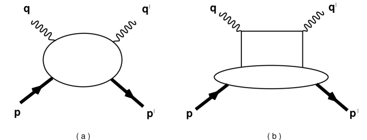
FIG. 2.: a). Compton scattering; b) Leading Feynman diagrams for DVCS.

The same DVCS final state can also be produced through the Bethe-Heitler process in which the initial or final state electron (or muon) radiates a real photon and at the same time scatters elastically off the target nucleon. This process can be calculated as accurately as the data on the nucleon elastic form factors. Physically, the Bethe-Heitler process is a background to DVCS and can overshadow the latter signal if the former is too large. On the other hand, with an appropriate size of Bethe-Heitler amplitude, one may hope to measure its interference with the DVCS amplitude which then can be directly extracted from data. The complete leading-order DVCS cross sections and the interference with the Bethe-Heitler amplitude can be found in Ref. [58].

Recently, Guichon made some interesting estimates of the cross sections at COMPASS and Jefferson Lab energies [67]. He found that while at low scattering energy, the Bethe-Heitler background is quite large, it drops significantly at high energies when the virtual photon flux is large. In fact, if one is focused on production of real photons along the direction of the virtual photon, the DVCS cross section is quite significant at COMPASS energy, and certainly far above the Bethe-Heitler background. As far as studying the orbital angular momentum of quarks is concerned, this is the most interesting kinematic region. Guichon’s estimate is encouraging for a real experiment.

The one-loop corrections to DVCS have recently been studied by Osborne and Ji[68]. They have also been studied by Müller [69] and by Belitsky and Müller [63] using the constraints from conformal symmetry. Results of these studies have been confirmed by Mankiewicz et al. [70]. Besides their obvious use in precision analysis, the results indicate that DVCS is factorizable at the next-to-leading order. A higher-order calculation of the coefficient functions in the renormalon-chain approximation has been done by Belitsky and Schäfer [71]. An all order proof of the DVCS factorization was first given by Radyushkin [30] and recently in a different perspective by Osborne and Ji [72], and Collins and Freund [73].

The simple DVCS scattering mechanism can be tested through scaling relations and selection rules, as in the case of deep-inelastic scattering. In Ref. [74], Diehl et al. considered the possibility of using $\phi$ dependence of the cross section to test the single quark scattering picture, where $\phi$ is the angle between the lepton and hadron scattering planes. They observed that through QCD radiative corrections, the photon helicity-flip amplitude may contribute to DVCS. A recent study by Hoodbhoy and Ji showed that this indeed happens [28]. The key element here is the helicity-flip off-forward gluon distributions, which decouple in the forward limit due to angular momentum conservation. They pointed out that a nonvanishing leading-twist photon helicity-flip amplitude signals unequivocally the presence of gluons in the nucleon.

There are other processes that are as clean as the DVCS, but more difficult to measure experimentally. For instance, $Z^{0}$ production was considered in Ref. [9]. Since $Z^{0}$’s are signaled through lepton pairs, one can also consider lepton-pair production through intermediate time-like virtual photons. Theoretical treatment of these is exactly the same as for DVCS.

B Vector Meson Production

Heavy quarkonium production was first considered by Ryskin as a way to measure the Feynman gluon distributions at small $x$ [11]. A leading-order diagram for the process is shown in Fig 3a, where the virtual photon fluctuates into a $c\bar{c}$ pair which subsequently scatters off the nucleon target through two-gluon exchanges. In the process, the pair transfers away certain amount of its longitudinal momentum and reduces its invariant mass to that of a $J/\Psi$. The cross section is,

$${d\sigma\over dt}(\gamma^{*}+P\rightarrow J/\Psi+P^{\prime})={16\pi^{3}M\Gamma_{e^{+}e^{-}}\over 3\alpha_{\rm em}Q^{6}}\alpha_{s}^{2}(\bar{Q}^{2})[\xi g(\xi,\bar{Q}^{2})]^{2}$$ (99)

where $\bar{Q}^{2}=(Q^{2}+M^{2})/4$, $M$ is the $J/\psi$ mass, and $\Gamma_{e^{+}e^{-}}$ is the decay width into the lepton pair. The equation was derived in the kinematic limit $s\gg Q^{2}\gg M^{2}\gg t$ and the Fermi motion of the quarks in the meson was neglected. Two other important approximations were used in the derivation. First, the contribution from the real part of the amplitude is neglected, which may be justifiable at small $x$. Second, the off-forward distributions are identified with the forward ones. As we have discussed in IV.A, even for small $t$, the approximation is good only if the off-diagonal evolution effects can be neglected. A more refined treatment of the process and comparison with HERA data can be found in Ref. [13].

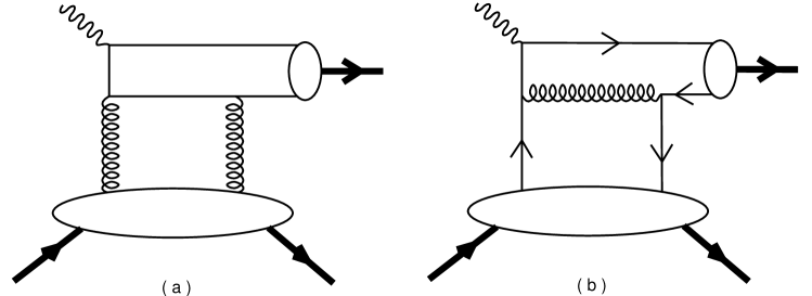
FIG. 3.: a). A representative Feynman diagram for neutral meson production through off-forward gluon distributions in the nucleon; b) A representative Feynman diagram for meson production through off-forward quark distributions in the nucleon.

The above result was extended to the case of light vector-meson production by Brodsky et al., who considered the effects of meson structure in perturbative QCD [12]. They found a similar cross section,

$$\left.{d\sigma\over dt}\right|_{t=0}(\gamma^{*}N\rightarrow VN)={4\pi^{3}\Gamma_{V}m_{V}\alpha_{s}^{2}(Q)\eta_{V}^{2}\left(xg(x,Q^{2})\right)^{2}\over 3\alpha_{\rm em}Q^{6}}\ ,$$ (100)

where the dependence on the meson structure is in the parameter

$$\eta_{V}={1\over 2}\int{dz\over z(1-z)}\phi^{V}(z)\left(\int dz\phi^{V}(z)\right)^{-1}\ ,$$ (101)

and $\phi^{V}(z)$ is the leading-twist light-cone wave function. Evidently, the above formula reduces to Ryskin’s in the heavy-quark limit $\left(\phi^{V}(x)=\delta(x-1/2)\right)$. More discussions on vector meson production along this line, including comparison with recent data, can be found in Ref. [13, 14, 75].

Radyushkin was the first to calculate the amplitude of hard diffractive electroproduction in terms of off-forward gluon distributions [23, 30]. With the virtual photon and vector meson both polarized longitudinally, his result corresponds to

$${d\sigma\over dt}(\gamma^{*}N\rightarrow VN)={4\pi\Gamma_{V}m_{V}\alpha_{s}^{2}(Q)\eta_{V}^{2}\over 3\alpha_{\rm em}Q^{6}}\left|2x_{B}\int^{1}_{-1}dx\left({1\over x-\xi+i\epsilon}+{1\over x+\xi-i\epsilon}\right)F_{g}(x,\xi,t)\right|^{2}\ ,$$ (102)

where again $x_{B}=2\xi/(1+\xi)$. The above formula is valid for any $x_{B}$ and $t$ smaller or around hadron mass scales. Hoodbhoy has also studied the effects of the off-forward distributions in the case of $J/\psi$ production [24]. He found that Ryskin’s result needs to be modified in a similar way once the off-forward effects becomes important.

Collins, Frankfurt, and Strikman have made an extensive analysis of the high-order QCD contributions to hard diffractive meson production [25]. Using the standard tools described in [3], they showed that the leading-twist contributions are factorizable to all orders in perturbation theory. The factorization theorem provides a rigorous QCD basis for calculating the process in terms of the off-forward distributions. In fact, the paper outlined a recipe for calculating a whole class of processes in perturbation theory. Mankiewicz, Piller and Weigl recently calculated the neutral pseudoscalar and vector meson production cross sections in terms of the non-forward quark and gluon distributions [70]. Shown in Fig. 3b is a Feynman diagram in which meson production depends on a quark distribution. They also investigated charged particle production in which the initial nucleon has a different charge from the final one [76]. The charge-changing off-forward distributions can be obtained from the charge-conserving ones using isospin symmetry. The result can be generalized to the octet baryons if the SU(3) flavor symmetry is good. One can also consider production of heavy-flavored baryons from the nucleon target. Unlike the heavy-quark distributions in light hadrons, the corresponding off-forward distributions are not suppressed by heavy-quark masses.

VI summary and outlook

The off-forward parton distributions are a new type of nucleon observables which have recently generated much interest in hadron physics community. On the one hand, the OFPD’s contain all the form factors of the twist-two operators which generalize the well-known electroweak currents. The form factors of the spin-two, twist-two operators (energy-momentum tensor) are especially interesting in unravelling the spin structure of the nucleon. On the other hand, they summarize succinctly the leading structural dependence in a class of high-energy processes involving the nucleon. The partonic interpretation of the OFPD’s is quite simple– it represents parton-nucleon scattering amplitudes on the light-cone.

Recent studies of the OFPD’s can largely be classified into three categories: modelling the new distributions, studying their scale dependences, and investigating processes that are sensitive to them. In terms of model studies, our accomplishments so far are rather limited. Even though there are bag and chiral soliton model calculations, these calculations need much improvement in the future. In particular, the physics in the $|x|<\xi$ region has not been entirely captured in these calculations. The models are yet to be extended to including gluon degrees of freedom which are known to be important even at low energy scales. Indeed, a vanishing helicity-flip gluon distribution at low-energy scales will remain zero at other scales because it has no mixing with any quark distribution. A number of rigorous constraints discussed in Section IV.A can be helpful in modelling: Apart from the special limits and $n=1$ moments, there exist useful upper bounds for the OFPD’s.

There have been many studies in perturbative evolution. At the leading-logarithmic level, evolution equations now have been obtained for all leading-twist OFPD’s. At next-to-leading order, one needs two-loop anomalous dimensions which exist only for the spin-independent non-singlet operators [77]. Calculations of additional two-loop anomalous dimensions will be needed as data on the OFPD’s become available. Recent works of Müller and Belitsky illustrate the power of exploiting the anomalous conformal symmetry to obtain these anomalous dimensions [78]. Numerical studies of evolution effects have just begun. Qualitatively we can understand the evolution effects from its asymptotic behavior. Quantitatively, one needs to establish high-precision, high-speed evolution codes which allow efficient data fitting in the future.

The leading-order cross sections for DVCS and meson production can be found in the literature. For DVCS, the cross section has also been computed to the next-to-leading order in $\alpha_{s}$. A similar study for meson production can be made, and will be necessary once precision data become available. Higher-twist effects are important at low $Q^{2}$ and must be

investigated thoroughly. Generally speaking, they are more complex to study than that in deep-inelastic scattering because of the extra photon or meson, and the extra soft scale $t$. Additional processes may be explored to probe the OFPD’s, including ones in which the final state baryon may contain strange or heavy flavors. Polarization observables need to be seriously investigated. A solid experimental confirmation of the scattering mechanisms involving the OFPD’s is itself very significant. It involves testing scaling relations and selection rules.

Finally, we notice that the OFPD’s are functions of multi-variables. As such, it would be difficult to get a complete picture of them in a short time period and in a single type of experiments. Moreover, experimental cross sections cannot be used to extract the distributions directly; they usually involve integrals over parton momenta. Therefore, it will be necessary to parametrize the OFPD’s and fit the parameters to data. In finding appropriate ways to make parametrizations and fits, model studies will play important role, unless of course lattice calculations can make a significant breakthrough in the near future.

Note Added: After this paper was submitted for publication, the author has noticed some new works in the literature which are relevant to the subject of this paper. In Ref. [79], Radyushkin studied both hadron form factors and wide-angle Compton scattering using nonforward parton densities. In Ref. [80], diffractive dijet photoproduction was proposed as a probe of the off-diagonal gluon distribution. In Ref. [81], certain positivity constraints for off-forward parton distributions were derived. In a different line of development, the orbital angular momentum distribution in the nucleon was investigated [82].

- [1] R. P. Feynman, Phys. Rev. Lett. 23 (1969) 1415; Photon Hadron Interactions, Benjamin, New York, 1972.
- [2] J. C. Collins, G. Sterman, and D. E. Soper, in Perturbative Quantum Chromodynamcis, ed. A. Mueller (World Scientific, Singapore, 1989)
- [3] J. C. Collins and D. E. Soper, Nucl. Phys. B194 (1982) 445.
- [4] See for instance, M. Creutz, Quarks, Gluons and Lattices (Cambridge Univ. Press, Cambridge, U.K., 1983)
- [5] M. Glück, E. Reya, and A. Vogt, Z. Phys. C 67 (1995) 433.
- [6] A. D. Martin, R. G. Roberts, and W. J. Stirling, Phys. Lett. B387 (1996) 419.
- [7] H. L. Lai et al., Phys. Rev. D55 (1997) 1280.
- [8] K. Watanabe, Prog. Theo. Phys. 67 (1982) 1834.
- [9] J. Bartels and M. Loewe, Z. Phys. C12 (1982) 263.
- [10] L. V. Gribov, E. M. Levin, and M. G. Ryskin, Phys. Rep. 100 (1983) 1.
- [11] M. G. Ryskin, Z. Phys. C37 (1993) 89.
- [12] S. J. Brodsky, L. L. Frankfurt, J. F. Gunion, A. H. Mueller, and M. Strikman, Phys. Rev. D50 (1994) 3134.
- [13] M. G. Ryskin, R. G. Roberts, A. D. Martin, and E. M. Levin, Zeit. Phys. C76 (1997) 231.
- [14] L. L. Frankfurt, W. Koepf, and M. Strikman, Phys. Rev. D54 (1996) 3194.
- [15] F. M. Dittes, D. Muller, D. Robaschik, B. Geyer, and J. Horejsi, Phys. Lett. B 209 (1988) 325.
- [16] V. N. Gribov and L. N. Lipatov, Sov. J. Nucl. Phys. 15 (1972) 78; G. Altarelli and G. Parisi, Nucl. Phys. B126 (1977) 298; Yu. L. Dokshitser, Sov. Phys. JETP 46 (1977) 641.
- [17] A. V. Efremov and A. V. Radyushkin, JINR-E2-11535, Dubna, 1978; A. V. Efremov and A. V. Radyushkin, Phys. Lett. B94 (1980) 245.
- [18] S. J. Brodsky and G. P. Lepage, Phys. Rev. D22 (1980) 2157.
- [19] D. Müller, D. Robaschik, B. Geyer, F.-M. Dittes, and J. Horejsi, Fortschr. Phys. 42 (1994) 101.
- [20] P. Jain and J. P. Ralston, in the proceedings of the workshop on Future Directions in Particle and Nuclear Physics at Multi-GeV Hadron Beam Facilities, BNL, March, 1993.
- [21] X. Ji, Phys. Rev. Lett. 78 (1997) 610.
- [22] H. Abramowicz, L. Frankfurt, and M. Strikman, DESY-95-047, SLAC Summer Inst. 1994, 539.
- [23] A. V. Radyushkin, Phys. Lett. B385 (1996) 333.
- [24] P. Hoodbhoy, Phys. Rev. D56 (1997) 388.
- [25] J. C. Collins, L. Frankfurt, and M. Strikman, Phys. Rev. D56 (1997) 2982.
- [26] C. Itzykson and J. Zuber, Quantum Field Theory, McGraw-Hill Inc., New York, 1980.
- [27] S. Brodsky and P. Lepage, in Perturbative Quantum Chromodynamcis, ed. A. Mueller (World Scientific, Singapore, 1989); See also X. Ji, Comm. Nucl. Part. Phys. 21 (1993) 123.
- [28] P. Hoodbhoy and X. Ji, hep-ph/9801369.
- [29] R. L. Jaffe and X. Ji, Nucl. Phys. B375 (1992) 527.
- [30] A. V. Radyushkin, Phys. Rev. D56 (1997) 5524.
- [31] A. V. Radyushkin, Phys. Lett. B380 (1996) 417.
- [32] G. Alteralli, R. D. Ball, S. Forte, and G. Ridolfi, Nucl. Phys. B496 (1997) 337.
- [33] M. Fukugita, Y. Kuramashi, M. Okawa, and A. Ukawa, Phys. Lett. 75 (1995) 2092.
- [34] S. J. Dong, J. F. Lagae, K. F. Liu, Phys. Rev. Lett. 75 (1995) 2096.
- [35] M. Göckeler et al., Phys. Rev. D53 (1996) 2317.
- [36] R. L. Jaffe and A. Manohar, Nucl. Phys. B337 (1990) 509.
- [37] L. Sehgal, Phys. Rev. D10 (1974) 1663.
- [38] P. G. Ratcliffe, Phys. Lett. B192 (1987) 180.
- [39] G. Altarelli and and G. G. Ross, Phys. Lett. B212 (1988) 391.
- [40] R. D. Carlitz, J. C. Collins, and A. H. Mueller, Phys. Lett. B214 (1988) 229.
- [41] X. Ji, hep-ph/9710290.
- [42] X. Ji, J. Tang, and P. Hoodbhoy, Phys. Rev. Lett. 76 (1996) 740.
- [43] D. Gross and F. Wilczek, Phys. Rev. D9 (1974) 980.
- [44] I. I. Balitsky and X. Ji, Phys. Rev. Lett. 79 (1997) 1225.
- [45] V. Barone, T. Calarco, A. Drago, hep-ph/9801281.
- [46] A. Martin and M. G. Ryskin, hep-ph/9711371, Phys. Rev. D57, June 1st 1998.
- [47] X. Ji, W. Melnitchouk, and X. Song, D56 (1997) 5511.
- [48] V. Yu. Petrov, P. V. Pobylitsa, M. V. Polyakov, I. Börnig, K. Goeke, and C. Weiss, hep/ph9710270.
- [49] A. W. Schreiber, A. I. Signal, A. W. Thomas, Phys. Rev. D44 (1991) 2653.
- [50] Yu. M. Makeenko, Sov. J. Nucl. Phys. 33 (1982) 440.
- [51] Th. Ohrndorf, Nucl. Phys. B198 (1982) 26.
- [52] M. K. Chase, Nucl. Phys. B174 (1980) 109;
- [53] Th. Ohrndorf, Nucl. Phys. B186 (1981) 153;
- [54] M. A. Shifman and M. Vysotsky, Nucl. Phys. B186 (1981) 475.
- [55] V. N. Baier and A. G. Grozin, Nucl. Phys. B192 (1981) 476.
- [56] B. Geyer, D. Robaschik, M. Bordag, and J. Horejsi, Z. Phys. C26 (1985) 591; I. Braunschweig, B. Geyer, J. Horejsi and D. Robaschik, Z. Phys. C33 (1987) 175.
- [57] I. I. Balitsky and V. M. Braun, Nucl. Phys. B311 (1988) 541.
- [58] X. Ji, Phys. Rev. D55 (1997) 7114.
- [59] Z. Chen, hep-ph/9705279.
- [60] L. L. Frankfurt, A. Freund, V. Guzey, and M. Strikman, hep-ph/9703449.
- [61] J. Blümlein, B. Geyer, and D. Robaschik, Phys. Lett. B413 (1997) 114.
- [62] I. I. Balitsky and A. V. Radyushkin, Phys. Lett. B413 (1997) 114.
- [63] A. V. Belitsky and D. Müller, hep-ph/9709379.
- [64] A. V. Belitsky, B. Geyer, D. Müller, and A. Schäfer, hep-ph/9710427.
- [65] L. Mankiewicz, G. Piller, and T. Weigl, hep-ph/9711227.
- [66] J. Crittenden, hep-ex/9709031.
- [67] P.A.M. Guichon, DAPNIA-SPHN-97-31, Talk given at 5th International Workshop on Deep Inelastic Scattering and QCD (DIS 97), Chicago, IL, 14-18 Apr 1997.
- [68] X. Ji and J. Osborne, Phys. Rev. D57 (1998) R1337.
- [69] D. Müller, hep-ph9704406, CERN-TH/97-80, 1997.
- [70] L. Mankiewicz, G. Piller, E. Stein, M. Vänttinen, T. Weigl, hep-ph/9712251.
- [71] A. V. Belitsky and A. Schäfer, hep-ph/9801252.
- [72] X. Ji and J. Osborne, hep-ph/9801260.
- [73] J. C. Collins and A. Freund, hep-ph/9801262.
- [74] M. Diehl, T. Gousset, B. Pire, and J. P. Ralston, Phys. Lett. B411 (1997) 193.
- [75] A. D. Martin, M. G. Ryskin, and T. Teubner, Phys.Rev. D55 (1997) 4239; D56 (1997) 3007.
- [76] L. Mankiewicz, G. Piller and T. Weigl, hep-ph/9712508.
- [77] F.-M. Dittes and A. V. Radyushkin, Phys. Lett. 134B (1984) 359; M. H. Sarmadi, ibid. 143B (1984) 471; G. R. Katz, Phys. Rev. D31 (1985) 652; S. V. Mikhailov and A. V. Radyushkin, Nucl. Phys. B254 (1985) 89.
- [78] D. Müller, Phys. Rev. D49 (1994) 2525; A. V. Belitsky and D. Müller, hep-ph/9802411.
- [79] A. V. Radyushkin, hep-ph/9803316.
- [80] K. Golec-Biernat, J. Kwiecinski, and A. D. Martin, hep-ph/9803464.
- [81] B. Pire, J. Soffer, and O. Teryaev, hep-ph/9804284.
- [82] P. Hägler and A. Schäfer, hep-ph/9802362; A. Harindranath and R. Kundu, hep-ph/9802406; O. V. Teryaev, hep-ph/9803403; P. Hoodbhoy, X. Ji, and W. Lu, hep-ph/9804337.