Radiative Corrections to $W$ and Quark
Propagators in the Resonance Region

Abstract

It is shown that conventional mass renormalization, when applied to photonic or gluonic corrections to unstable particle propagators, leads to non-convergent series in the resonance region. A solution of this problem, based on the concepts of pole mass and width, is presented. In contrast with the $Z$ case, the conventional on-shell definition of mass for $W$ bosons and unstable quarks contains an unbounded gauge dependence in next-to-leading order. The on-shell and pole definitions of width are shown to coincide if terms of $O(\Gamma^{2})$ and higher are neglected, but not otherwise.

PACS numbers: 12.15.Lk, 11.10.Gh, 11.15.Bt, 14.70.Fm

NYU-TH/98-06-01
June 1998

1 Introduction

Theoretical arguments advanced in 1991 led to the conclusion that, in the $Z$ case, the on-shell mass

$$M^{2}=M_{0}^{2}+\mbox{Re}A(M^{2}),$$ (1)

is gauge dependent in $O(g^{4})$ and higher [1, 2]. If the arguments are correct one should see the gauge dependence in the analysis of the $Z$ resonant amplitude propagator or, equivalently, in the study of the $Z$ line shape. This was, in fact, confirmed [3, 4]. The situation in $O(g^{4})$ is particularly simple to see. Calling $\widetilde{M}_{{\scriptscriptstyle Z}}$ the observed $Z$-mass, one finds

$$\widetilde{M}_{{\scriptscriptstyle Z}}^{2}=M_{\scriptscriptstyle Z}^{2}+M_{\scriptscriptstyle Z}\Gamma_{{\scriptscriptstyle Z}}\left[\mbox{Im}A^{\prime}_{b}(M_{\scriptscriptstyle Z}^{2})-\frac{9G_{\mu}m_{b}^{2}}{12\pi\sqrt{2}}\right]+O(g^{6}),$$ (2)

where $M_{\scriptscriptstyle Z}$ is the on-shell mass (Cf. Eq. (1.1)), $A_{b}(M_{\scriptscriptstyle Z}^{2})$ is the bosonic contribution to the $Z$ self-energy, the prime indicates differentiation with respect to $s$, and the term proportional to $G_{\mu}m_{b}^{2}$ represents a very small violation to the scaling behavior $\mbox{Im}A_{f}(s)\sim s$ ($A_{f}(s)$ is the fermionic contribution to the self-energy). $\mbox{Im}A^{\prime}_{b}(M_{\scriptscriptstyle Z}^{2})$ is different from zero and $\xi_{\scriptscriptstyle W}$-dependent when $M_{\scriptscriptstyle Z}\geq 2M_{\scriptscriptstyle W}\sqrt{\xi_{\scriptscriptstyle W}}$ or $\xi_{\scriptscriptstyle W}\leq 1/4\cos^{2}\theta_{{\scriptscriptstyle W}}$. There is a second class of contributions to $\mbox{Im}A^{\prime}_{b}(M_{\scriptscriptstyle Z}^{2})$ when $M_{\scriptscriptstyle Z}\geq M_{\scriptscriptstyle W}(1+\sqrt{\xi_{\scriptscriptstyle W}})$ or $\xi_{\scriptscriptstyle W}\leq[(1/\cos\theta_{{\scriptscriptstyle W}})-1]^{2}$. One finds $|\mbox{Im}A^{\prime}_{b}(M_{\scriptscriptstyle Z}^{2})|_{max}=1.6\times 10^{-3}$ very near the threshold of the second contribution. Thus, in $O(g^{4})$ the gauge dependence of $M_{\scriptscriptstyle Z}$ is bounded and amounts to a maximum of $2\mbox{ MeV}$. Although very small, this is of the same magnitude as the current experimental error. Instead, in $O(g^{6})$ the gauge dependence of $M_{\scriptscriptstyle Z}$ is unbounded.

Another definition that plays an important role is based on the complex-valued position of the pole [5, 1, 2, 3]:

$$\overline{s}=M_{0}^{2}+A(\overline{s}),\quad\overline{s}=m_{2}^{2}-im_{2}\Gamma_{2}.$$ (3)

An important property is that $m_{2}$ and $\Gamma_{2}$ are gauge-independent. In particular,

$$m_{1}=\sqrt{m_{2}^{2}+\Gamma_{2}^{2}}$$ (4)

can be identified with the mass measured at LEP [1, 2].

2 $W$ and Quark Propagators in the Resonance Region

A very recent work has extended the analysis to $W$ and quark propagators in the resonant region [6].

One finds that a new problem emerges: in the treatment of the photonic corrections, conventional mass-renormalization generates, in next-to-leading order (NLO), a series in powers of $M\Gamma/(s-M^{2})$, which does not converge in the resonance region! Furthermore, it diverges term-by-term at $s=M^{2}$. This problem is generally present whenever the unstable particle is coupled to massless quanta. Aside from the $W$, an interesting example is the QCD correction to a quark propagator when the weak interactions are switched on, so that the quark becomes unstable. In Ref. [6] a solution of this serious problem is presented in the framework of the complex pole formalism.

In order to illustrate the difficulties emerging in the resonance region when conventional mass renormalization is employed, we consider the contribution of the transverse part of the $W$ propagator in the loop of Fig. (1), which contains $l$ self-energy insertions.

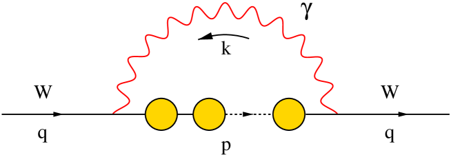
Fig. 1: A class of photonic corrections to the $W$ self-energy. The inner solid and dashed lines and blobs represent transverse $W$ propagators and self-energies.

Calling

$$\Pi^{\scriptscriptstyle(T)}_{\mu\nu}(q)=t_{\mu\nu}(q)A(s),$$ (1)

the transverse $W$ self-energy, where $s\equiv q^{2}$ and $t_{\mu\nu}(q)=$ $g_{\mu\nu}-q_{\mu}q_{\nu}/q^{2}$, the contribution $A_{{\scriptscriptstyle W}\gamma}^{(l)}(s)$ from Fig. (1) to $A(s)$ is given by

$$A_{{\scriptscriptstyle W}\gamma}^{(l)}(s) = ie^{2}(\mu)\,\frac{t_{\mu\nu}(q)}{(n-1)}\,\mu^{4-n}$$

$$\times \!\!\!\!\!\!\!\!\!\!\!\!\int\frac{d^{n}\!k}{(2\pi)^{n}}{\cal{D}}^{{\scriptscriptstyle(}\gamma{\scriptscriptstyle)}}_{\rho\beta}(k){\cal{D}}^{\scriptscriptstyle(W,T)}_{\lambda\alpha}(p){\cal{V}}^{\rho\lambda\nu}{\cal{V}}^{\beta\alpha\mu}\left[\frac{A^{{\scriptscriptstyle(}s{\scriptscriptstyle)}}(p^{2})}{p^{2}-M^{2}+i\epsilon}\right]^{l},$$ (2)

where $p=q+k$ is the $W$ loop-momentum,

$${\cal D}^{{\scriptscriptstyle(}\gamma{\scriptscriptstyle)}}_{\rho\beta}(k)=-\frac{i}{k^{2}}\left(g_{\rho\beta}+(\xi_{\gamma}-1)\frac{k_{\rho}k_{\beta}}{k^{2}}\right),$$ (3)

$${\cal D}^{\scriptscriptstyle(W,T)}_{\lambda\alpha}(p)=\frac{-i}{p^{2}-M^{2}+i\epsilon}\left(g_{\alpha\lambda}-\frac{p_{\alpha}p_{\lambda}}{p^{2}}\right),$$ (4)

$${\cal V}^{\beta\alpha\mu}=(2p-k)^{\beta}g^{\alpha\mu}+(2k-p)^{\alpha}g^{\beta\mu}-(k+p)^{\mu}g^{\beta\alpha},$$ (5)

$\xi_{\gamma}$ is the photon gauge parameter and $A^{{\scriptscriptstyle(}s{\scriptscriptstyle)}}(p^{2})$ stands for the $W$ transverse self-energy with the conventional mass renormalization subtraction:

$$A^{{\scriptscriptstyle(}s{\scriptscriptstyle)}}(p^{2}) = \mbox{Re}\left(A(p^{2})-A(M^{2})\right)+i\mbox{Im}A(p^{2})$$ (6)

$$= A(p^{2})-A(M^{2})+i\mbox{Im}A(M^{2}).$$

We note that each insertion of $A^{{\scriptscriptstyle(}s{\scriptscriptstyle)}}(p^{2})$ is accompanied by an additional denominator $[p^{2}-M^{2}+i\epsilon]$. Thus, Eq. (2.2) may be regarded as the $l$th term in an expansion in powers of

$$\left[A(p^{2})-A(M^{2})+i\mbox{Im}A(M^{2})\right]\left(p^{2}-M^{2}+i\epsilon\right)^{-1}.$$

As $A(p^{2})-A(M^{2})=O[g^{2}(p^{2}-M^{2})]$ for $p^{2}\approx M^{2}$, the contribution $[A(p^{2})-A(M^{2})]$ $(p^{2}-M^{2}+i\epsilon)^{-1}$ is of $O(g^{2})$ throughout the region of integration. However, as $i\mbox{Im}A(M^{2})\approx-iM\Gamma$ is not subtracted, the combination $i\mbox{Im}A(M^{2})/(p^{2}-M^{2}+i\epsilon)$ may lead to terms of $O(1)$ if the domain of integration $|p^{2}-M^{2}|$ $\stackrel{{\scriptstyle\textstyle<}}{{\sim}}\,$$M\Gamma$ is important. In fact, the contribution of $[i\mbox{Im}A(M^{2})/(p^{2}-M^{2}+i\epsilon)]^{l}$ to Eq. (2.2) is, to leading order,

$$A_{{\scriptscriptstyle W}\gamma}^{(l)}(s)=\frac{(-iM\Gamma)^{l}}{l!}\frac{d^{l}}{d(M^{2})^{l}}A_{{\scriptscriptstyle W}\gamma}^{(0)}(s)+\ldots,$$ (7)

where $A_{{\scriptscriptstyle W}\gamma}^{(0)}(s)$ represents the diagram with no self-energy insertions and the dots indicate additional contributions not relevant to our argument.

In the resonance region $|s-M^{2}|$ $\stackrel{{\scriptstyle\textstyle<}}{{\sim}}\,$$M\Gamma$ the zeroth order propagator is inversely proportional to $(s-M^{2}+iM\Gamma)=O(g^{2})$. In NLO, contributions of $O[\alpha(s-M^{2}),\alpha M\Gamma]$ are therefore retained but those of $O[\alpha(s-M^{2})^{2}]$ are neglected. Explicit evaluation of $A_{{\scriptscriptstyle W}\gamma}^{(0)}(s)$ in NLO leads to

$$A_{{\scriptscriptstyle W}\gamma}^{(0)}(s)=\frac{\alpha}{2\pi}\left[(\xi_{\gamma}-3)(s-M^{2})\ln\!\left(\frac{M^{2}-s}{M^{2}}\right)+\ldots\right].$$ (8)

Inserting Eq. (2.8) into Eq. (2.7) we obtain

$$A_{{\scriptscriptstyle W}\gamma}^{(1)}(s) = \frac{\alpha}{2\pi}(\xi_{\gamma}-3)\left(iM\Gamma\right)\left[\ln\!\left(\frac{M^{2}-s}{M^{2}}\right)+\frac{s}{M^{2}}\right]+\ldots,$$

$$A_{{\scriptscriptstyle W}\gamma}^{(l)}(s) = \frac{\alpha}{2\pi}(\xi_{\gamma}-3)\frac{(s-M^{2})}{l(l-1)}\left(\frac{-iM\Gamma\phantom{{}^{2}}}{s-M^{2}}\right)^{\!l}+\ldots,\quad(l\geq 2).$$ (9)

As in the resonance region all these terms contribute in NLO, conventional mass renormalization leads in NLO to a series in powers of $M\Gamma/(s-M^{2})$, which does not converge in the resonance region. Rather than generating contributions of higher order in $g^{2}$, each successive self-energy insertion gives rise to a factor $-iM\Gamma/(s-M^{2})$, which is nominally of $O(1)$ in the resonance region and furthermore diverges at $s=M^{2}$!

One possibility would be to resum the series $\sum^{\infty}_{l=0}A_{{\scriptscriptstyle W}\gamma}^{(l)}(s)$ with $A_{{\scriptscriptstyle W}\gamma}^{(l)}(s)$ given by Eq. (2.7). This would lead to

$$\sum^{\infty}_{l=0}A_{{\scriptscriptstyle W}\gamma}^{(l)}(s,M^{2})=A_{{\scriptscriptstyle W}\gamma}^{(0)}(s,M^{2}-iM\Gamma)+\ldots,$$ (10)

or

$$\sum^{\infty}_{l=0}A_{{\scriptscriptstyle W}\gamma}^{(l)}(s)=\frac{\alpha}{2\pi}\left[(\xi_{\gamma}-3)(s-M^{2}+iM\Gamma)\ln\left(\frac{M^{2}-iM\Gamma-s}{M^{2}-iM\Gamma}\right)+\ldots\right].$$ (11)

Even if one accepts these resummations rather than the usual term by term expansions, the theoretical situation in the conventional formalism is very unsatisfactory. In fact, in the conventional formalism, the $W$ propagator is inversely proportional to

$${\cal D}^{-1}(s)=s-M^{2}+iM\Gamma-\left(A(s)-A(M^{2})\right)-iM\Gamma\,\mbox{Re}A^{\prime}(M^{2}),$$ (12)

where $\Gamma$ is the radiatively corrected width and we have employed its conventional expression

$$M\Gamma=-\mbox{Im}A(M^{2})/[1-\mbox{Re}A^{\prime}(M^{2})].$$ (13)

The contribution of the $(s-M^{2}+iM\Gamma)\ln[(M^{2}-iM\Gamma-s)/(M^{2}-iM\Gamma)]$ term to ${\cal D}^{-1}(s)$ is

$$-\frac{\alpha}{2\pi}(\xi_{\gamma}-3)\left[(s-M^{2}+iM\Gamma)\ln\left(\frac{M^{2}-iM\Gamma-s}{M^{2}-iM\Gamma}\right)+iM\Gamma\left(1+i\frac{\pi}{2}\right)\right]$$

and we note that the last term is a gauge-dependent contribution not proportional to the zeroth order term $s-M^{2}+iM\Gamma$. As a consequence, in NLO the pole position is shifted to ${\widetilde{M}}^{2}-i\widetilde{M}\widetilde{\Gamma}$, where

$${\widetilde{M}}^{2} = M^{2}[1-(\alpha/4)(\xi_{\gamma}-3)(\Gamma/M)],$$ (14)

$$\widetilde{\Gamma} = \Gamma[1-(\alpha/2\pi)(\xi_{\gamma}-3)].$$ (15)

As the pole position is gauge-invariant, so must be $\widetilde{M}$ and $\widetilde{\Gamma}$. Furthermore, in terms of $\widetilde{M}$ and $\widetilde{\Gamma}$, ${\cal D}^{-1}(s)$ retains the Breit–Wigner structure. Thus, in a resonance experiment $\widetilde{M}$ and $\widetilde{\Gamma}$ would be identified with the mass and width of $W$.

The relation $\widetilde{\Gamma}=\Gamma[1-(\alpha/2\pi)(\xi_{\gamma}-3)]$ leads to a contradiction: the measured, gauge-independent, width $\widetilde{\Gamma}$ would differ from the theoretical value $\Gamma$ by a gauge-dependent quantity in NLO! This contradicts the premise of the conventional formalism that $\Gamma$, defined in Eq. (2.13), is the radiatively corrected width and is, furthermore, gauge-independent. We can anticipate that the root of this clash between the resummed expression and the conventional definition of width is that the latter is only an approximation. In particular, it is not sufficiently accurate when non-analytic contributions are considered.

A good and consistent formalism may circumvent awkward resummations of non-convergent series and should certainly avoid the above discussed contradictions. To achieve this, we return to the transverse dressed $W$ propagator, inversely proportional to $p^{2}-M_{0}^{2}-A(p^{2})$. In the conventional mass renormalization one eliminates $M^{2}_{0}$ by means of the expression $M^{2}_{0}=M^{2}-\mbox{Re}A(M^{2})$ (Cf. Eq. (1.1)). An alternative possibility is to eliminate $M^{2}_{0}$ by means of $M^{2}_{0}=\overline{s}-A(\overline{s})$ (Cf. Eq. (1.3)). The dressed propagator in the loop integral is inversely proportional to $p^{2}-\overline{s}-[A(p^{2})-A(\overline{s})]$. Its expansion about $p^{2}-\overline{s}$ generates in Fig. (1) a series in powers of $[A(p^{2})-A(\overline{s})]/(p^{2}-\overline{s})$. As $A(p^{2})-A(\overline{s})=O[g^{2}(p^{2}-\overline{s})]$ when the loop momentum is in the resonance region, $[A(p^{2})-A(\overline{s})]/(p^{2}-\overline{s})$ is $O(g^{2})$ throughout the domain of integration. Thus, each successive self-energy insertion leads now to terms of higher order in $g^{2}$ without awkward non-convergent contributions. In this modified strategy, the zeroth order propagator in Eq. (2.4) is replaced by

$${\cal D}^{\scriptscriptstyle(W,T)}_{\alpha\lambda}(p)=\frac{-i}{p^{2}-\overline{s}}\left(g_{\alpha\lambda}-\frac{p_{\alpha}p_{\lambda}}{p^{2}}\right).$$ (16)

The poles in the $k^{0}$ complex plane remain in the same quadrants as in Feynman’s prescription and Feynman’s contour integration or Wick’s rotation can be carried out. $A_{{\scriptscriptstyle W}\gamma}^{(0)}(s)$, Fig. (1) without loop insertions, now leads directly to

$$A_{{\scriptscriptstyle W}\gamma}^{(0)}(s)=\frac{\alpha}{2\pi}\left[(\xi_{\gamma}-3)(s-\overline{s})\ln\!\left(\frac{\overline{s}-s}{\overline{s}}\right)+\ldots\right],$$ (17)

which has the same structure as the expression we obtained in the conventional approach after resumming a non-convergent series. $A_{{\scriptscriptstyle W}\gamma}^{(l)}(s)$ ($l\geq 1$), the contributions with $l$ insertions in Fig. (1), are now of $O(\alpha g^{2l})$, the normal situation in perturbative expansions. The $W$ propagator in the modified formalism is inversely proportional to $s-\overline{s}-[A(s)-A(\overline{s})]$. As $A_{{\scriptscriptstyle W}\gamma}^{(0)}(s)$ is now proportional to $s-\overline{s}$, the pole position is not displaced, the gauge-dependent contributions factorize as desired, and the above discussed pitfalls are avoided. $A_{{\scriptscriptstyle W}\gamma}^{(l)}(s)$ leads now to contributions to $[A(s)-A(\overline{s})]$ of order $O[(s-\overline{s})\alpha g^{2l}]=O[\alpha g^{2(l+1)}]$ in the resonance region and can therefore be neglected in NLO for $l\geq 1$. We note that the $\ln[(\overline{s}-s)/\overline{s}]$ term in Eq. (2.17) cancels for $\xi_{\gamma}=3$, the gauge introduced by Fried and Yennie in Lamb-shift calculations [7].

The remaining contributions to $A(s)$ from the photonic diagrams, including those from the longitudinal part of the $W$ propagator in Fig. (1), and from the diagrams involving the unphysical scalars $\phi$ and the ghost $C_{\gamma}$, have no singularities at $s=M^{2}$ and can therefore be studied with conventional methods. In particular, in the evaluation of $A(s)-A(\overline{s})$ in NLO it is sufficient to retain their one-loop contributions. In these diagrams the propagators are proportional to $(p^{2}-M^{2}\xi_{\scriptscriptstyle W})^{-1}$ rather than $(p^{2}-M^{2})^{-1}$. As a consequence, they lead to logarithmic terms proportional to

$$(s-M^{2})\left[\frac{s-M^{2}\xi_{\scriptscriptstyle W}}{M^{2}}\right]\ln\!\left(\frac{M^{2}\xi_{\scriptscriptstyle W}-s}{M^{2}\xi_{\scriptscriptstyle W}}\right).$$

(The occurrence of branch cuts starting at $s=M^{2}\xi_{\scriptscriptstyle W}$ indicates the unphysical nature of these singularities.) In the resonance region, in NLO, these terms can be replaced by $(s-M^{2})(1-\xi_{\scriptscriptstyle W})\ln[(\xi_{\scriptscriptstyle W}-1)/\xi_{\scriptscriptstyle W}]$ [6].

Calling $A^{\gamma}(s)$ the overall contribution of the one-loop photonic diagrams to the transverse $W$ self-energy (Fig. (2)), in the modified formulation the relevant quantity in the correction to the $W$ propagator is $A^{\gamma}(s)-A^{\gamma}(\overline{s})$. The corresponding one-loop gluonic contribution to the quark self-energy is depicted in Fig. (3). In general $R_{\xi}$ gauge, we find in NLO

$$A^{\gamma}(s)-A^{\gamma}(\overline{s})=\frac{\alpha(m_{2})}{2\pi}(s-\overline{s})\left\{\delta\left(\frac{\xi_{\scriptscriptstyle W}}{2}-\frac{23}{6}\right)+\frac{34}{9}-2\ln\!\left(\frac{\overline{s}-s}{\overline{s}}\right)\right.$$

$$\!\!\!\!\!\!\!\!\!\!-\left(\xi_{\scriptscriptstyle W}-1\right)\left[\frac{\xi_{\scriptscriptstyle W}}{12}-\left(1-\frac{(\xi_{\scriptscriptstyle W}-1)^{2}}{12}\right)\ln\!\left(\frac{\xi_{\scriptscriptstyle W}-1}{\xi_{\scriptscriptstyle W}}\right)\right]-\left(\frac{11}{12}-\frac{\xi_{\scriptscriptstyle W}}{4}\right)\ln\xi_{\scriptscriptstyle W}$$

$$\!\!\!\!\!\!\!\!\!\!\left.+\left(\xi_{\gamma}-1\right)\left[\frac{\delta}{2}+\frac{1}{2}+\ln\!\left(\frac{\overline{s}-s}{\overline{s}}\right)+\frac{(\xi_{\scriptscriptstyle W}^{2}-1)}{4}\ln\!\left(\frac{\xi_{\scriptscriptstyle W}-1}{\xi_{\scriptscriptstyle W}}\right)-\frac{\ln\xi_{\scriptscriptstyle W}}{4}+\frac{\xi_{\scriptscriptstyle W}}{4}\right]\right\},$$

where $\delta=(n-4)^{-1}+(\gamma_{E}-\ln 4\pi)/2$, we have treated the logarithmic terms according to the previous discussion and set $\mu=m_{2}$. The full one-loop expression for $A^{\gamma}(s)$ in general $R_{\xi}$ gauges without using the NLO approximation is given in Ref. [6]. Of particular interest in Eq. (LABEL:eq:Agamma-Agamma) is the log term

$$\frac{\alpha(m_{2})}{2\pi}\left(\xi_{\gamma}-3\right)\left(s-\overline{s}\right)\ln\!\left(\frac{\overline{s}-s}{\overline{s}}\right),$$

which is independent of $\xi_{\scriptscriptstyle W}$ but is proportional to $(\xi_{\gamma}-3)$.

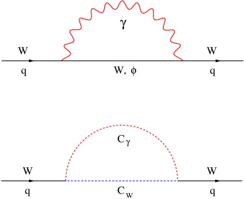
Fig. 2: One-loop photonic diagrams for the $W$ self-energy; $\phi$ is the unphysical scalar, $C_{\gamma}$ and $C_{W}$ are ghosts.

Writing

$$1-\frac{s}{\overline{s}}=1-\frac{s}{m_{1}^{2}}-i\frac{s}{m_{1}^{2}}\frac{\Gamma_{2}}{m_{2}}=\rho e^{i\theta},$$ (19)

we have

$$\rho(s)=\left[\left(1-\frac{s}{m_{1}^{2}}\right)^{2}+\frac{s^{2}\Gamma_{2}^{2}}{m_{1}^{4}m_{2}^{2}}\right]^{1/2},$$ (20)

$$\rho\sin\theta(s)=-\frac{s\Gamma_{2}}{m_{1}^{2}m_{2}}.$$ (21)

In Figs. (4,5), the functions $\ln\rho(s)$ and $\theta(s)$ are plotted for $m_{1}=80.4\mbox{ GeV}$ and $\Gamma_{1}=\Gamma_{2}m_{1}/m_{2}=2\mbox{ GeV}$ over a large range of $\sqrt{s}$ values. Figs. (6,7) compare these functions with the zero-width approximations over the resonance region. We note that the zero width approximation,

$$\mbox{Im}\left[\ln\!\left(\frac{M^{2}-s-i\epsilon}{M^{2}}\right)\right]=-\pi\theta\left(s-M^{2}\right),$$

is not valid in the resonance region. The logarithm $\ln(\xi_{\scriptscriptstyle W}-1)$ in Eq. (LABEL:eq:Agamma-Agamma) contains an imaginary contribution $-i\pi\theta(1-\xi_{\scriptscriptstyle W})$. This can be understood from the observation that, for $\xi_{\scriptscriptstyle W}<1$, a $W$ boson of mass $s=M^{2}$ has non-vanishing phase space to “decay” into a photon and particles of mass $M^{2}\xi_{\scriptscriptstyle W}$.

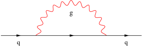
Fig. 3: One loop diagram for the quark self-energy in QCD.

3 Gauge Dependence of the On-Shell Mass

The difference between the pole mass $m_{1}$, defined in Eq. (1.4), and the conventional on-shell mass $M$, defined in Eq. (1.1), is

$$M^{2}-m_{1}^{2}=\mbox{Re}A(M^{2})-\mbox{Re}A(\overline{s})-\Gamma_{2}^{2}.$$ (1)

The contribution of the $(s-\overline{s})\ln[(\overline{s}-s)/\overline{s}]$ term to the r.h.s. of Eq. (3.1) is

$$\frac{\alpha(m_{2})}{2\pi}\left(\xi_{\gamma}-3\right)\left[\left(M^{2}-m_{2}^{2}\right)\mbox{Re}\ln\!\left(\frac{\overline{s}-M^{2}}{\overline{s}}\right)-m_{2}\Gamma_{2}\mbox{Im}\ln\!\left(\frac{\overline{s}-M^{2}}{\overline{s}}\right)\right]$$ (2)

$$\approx \frac{\alpha(m_{2})}{2\pi}\left(\xi_{\gamma}-3\right)\left[\left(M^{2}-m_{1}^{2}\right)\mbox{Re}\ln\!\left(\frac{\overline{s}-M^{2}}{\overline{s}}\right)+m_{2}\Gamma_{2}\frac{\pi}{2}\right].$$

In $\mbox{Im}\ln[(\overline{s}-M^{2})/\overline{s}]$ we have approximated $M^{2}\approx m_{1}^{2}$ and used the fact that $\theta=-\pi/2$ for $s=m_{1}^{2}$. Thus, we have

$$M^{2}-m_{1}^{2}=\frac{\alpha(m_{2})}{4}(\xi_{\gamma}-3)m_{2}\Gamma_{2}+\ldots,$$ (3)

where the dots indicate additional contributions. We note that this last equation corresponds to our previous result from the propagator, Eq. (2.14), with the identification $\widetilde{M}\rightarrow m_{1}$. In particular, Eq. (3.3) leads to $m_{1}-M=\alpha(m_{2})\Gamma_{2}/4\approx 4\mbox{ MeV}$ in the frequently employed ’t Hooft–Feynman gauge $(\xi_{i}=1)$, and to $\approx 6\mbox{ MeV}$ in the Landau gauge $(\xi_{i}=0)$. The contribution to $M^{2}-m_{1}^{2}$ from the term proportional to $(s-\overline{s})(\xi_{\gamma}-1)(\xi_{\scriptscriptstyle W}^{2}-1)\ln(\xi_{\scriptscriptstyle W}-1)$ (Cf. Eq. (LABEL:eq:Agamma-Agamma)) is $(\alpha/8)(\xi_{\gamma}-1)M\Gamma(\xi_{\scriptscriptstyle W}^{2}-1)\,\theta(1-\xi_{\scriptscriptstyle W})$, which is unbounded in $\xi_{\gamma}$ but restricted to $\xi_{\scriptscriptstyle W}<1$. In analogy with the $Z$ case, there are also bounded gauge-dependent contributions to $m_{1}-M$ arising from non-photonic diagrams in the restricted range $M_{\scriptscriptstyle W}>M_{\scriptscriptstyle Z}\sqrt{\xi_{\scriptscriptstyle Z}}+M_{\scriptscriptstyle W}\sqrt{\xi_{\scriptscriptstyle W}}$ or $\sqrt{\xi}_{\scriptscriptstyle Z}\leq\cos\theta_{\mbox{\footnotesize{w}}}[1-\sqrt{\xi}_{\scriptscriptstyle W}]$, and from the photonic corrections proportional to $(\xi_{\scriptscriptstyle W}-1)\ln[(\xi_{\scriptscriptstyle W}-1)/\xi_{\scriptscriptstyle W}]$ (Cf. Eq. (LABEL:eq:Agamma-Agamma)).

The following observation is appropriate at this point. In calculating the fundamental observable $\Delta r$ [8] (and its $\overline{\mbox{MS}}$ counterparts, $\Delta\hat{r}$ [9] and $\Delta\hat{r}_{\scriptscriptstyle W}$ [10]), the use of $M^{2}$ should produce a gauge dependence in $O(\alpha g^{2})$ in the radiative corrections. How is this possible if $\Delta r$ involves $A(s)\approx A(0)$? The point is that it also involves the counterterm $\mbox{Re}A(M^{2})$. If one employs the resummed expression $(\alpha/2\pi)(\xi_{\gamma}-3)(s-M^{2}+iM\Gamma)\ln[(M^{2}-iM\Gamma-s)/(M^{2}-iM\Gamma)]$, it gives a contribution $(\alpha/2\pi)(\xi_{\gamma}-3)M\Gamma$ to $\mbox{Re}A(M^{2})$. If one does not use the resummed expression, one gets the same result from the graph of Fig. (1) with one self-energy insertion ($l=1$), provided one defines $\theta(0)=1/2$ in accordance with the $i\epsilon$ prescription. One should eliminate such terms by means of the replacement $M^{2}-(\alpha/4)(\xi_{\gamma}-3)M\Gamma=m_{1}^{2}$ and identify $m_{1}$ with the measured mass.

4 Overall Corrections to $W$ Propagators in the Resonance Region

In contrast with the photonic corrections, the non-photonic contributions $A_{np}(s)$ to $A(s)$ are analytic around $s=\overline{s}$. In NLO we can therefore write

$$A_{np}(s)-A_{np}(\overline{s})=(s-\overline{s})A_{np}^{\prime}(m_{2}^{2})+\ldots,$$ (1)

where the dots indicate higher-order contributions.

In the resonance region, and in NLO, the transverse $W$ propagator becomes

$${\cal D}^{\scriptscriptstyle(W,T)}_{\alpha\beta}(q)=\frac{-i\left(g_{\alpha\beta}-q_{\alpha}q_{\beta}/q^{2}\right)}{\left(s-\overline{s}\right)\left[1-A_{np}^{\prime}(m_{2}^{2})-\frac{\alpha(m_{2})}{2\pi}F(s,\overline{s},\xi_{\gamma},\xi_{\scriptscriptstyle W})\right]},$$ (2)

where $s=q^{2}$ and $F(s,\overline{s},\xi_{\gamma},\xi_{\scriptscriptstyle W})$ is the expression between curly brackets in Eq. (LABEL:eq:Agamma-Agamma). An alternative expression, involving an $s-$dependent width, can be obtained by splitting $A_{np}^{\prime}$ into real and imaginary parts, and the latter into fermionic Im$A^{\prime}_{f}$ and bosonic Im$A^{\prime}_{b}$ contributions. Neglecting very small scaling violations, we have

$$\mbox{Im}A^{\prime}_{f}(m_{2}^{2})\approx\mbox{Im}A_{f}(m_{2}^{2})/m_{2}^{2}\approx-\Gamma_{2}/m_{2}$$ (3)

and

$${\cal D}^{\scriptscriptstyle(W,T)}_{\alpha\beta}(q)=\frac{-i\left(g_{\alpha\beta}-q_{\alpha}q_{\beta}/q^{2}\right)}{\left(s-m_{1}^{2}+is\frac{\Gamma_{1}}{m_{1}}\right)\left[1-\mbox{Re}A_{np}^{\prime}(m_{1}^{2})-i\mbox{Im}A_{b}^{\prime}(m_{1}^{2})-\frac{\alpha(m_{1})}{2\pi}F\right]},$$ (4)

where $\Gamma_{1}/m_{1}=\Gamma_{2}/m_{2}$. $\mbox{Im}A_{b}^{\prime}(m_{1}^{2})$ is non-zero and gauge-dependent in the subclass of gauges that satisfy $\sqrt{\xi}_{\scriptscriptstyle Z}\leq\cos\theta_{\mbox{\footnotesize{w}}}[1-\sqrt{\xi}_{\scriptscriptstyle W}]$. Otherwise $\mbox{Im}A_{b}^{\prime}(m_{1}^{2})$ vanishes. Although $m_{1}$ and $\Gamma_{1}$ are gauge-invariant, $\mbox{Re}A^{\prime}_{np}(m_{1}^{2})$, $\mbox{Im}A^{\prime}_{np}(m_{1}^{2})$ and $F$ are gauge-dependent. In physical amplitudes, such gauge-dependent terms cancel against contributions from vertex and box diagrams. The crucial point is that the gauge-dependent contributions in Eq. (4.4) factorize so that such cancelations can take place and the position of the complex pole is not displaced.

5 Comparison of the $W$ Width in the Conventional and Modified Formulations

Calling $A_{0}(s,M^{2}_{0})$ the transverse self-energy evaluated in terms of the bare mass $M_{0}$, and $A(s,M^{2})$ and $\bar{A}(s,\overline{s})$ the expressions obtained by substituting $M_{0}^{2}=M^{2}-\mbox{Re}A(M^{2},M^{2})$ and $M_{0}^{2}=\overline{s}-\bar{A}(\overline{s},\overline{s})$, respectively, we have

$$A_{0}(s,M^{2}_{0})=A(s,M^{2})=\bar{A}(s,\overline{s}).$$ (1)

In the conventional approach the $W$ width is given by Eq. (2.13) or, equivalently,

$$M\Gamma=-\mbox{Im}A(M^{2},M^{2})+M\Gamma\,\mbox{Re}A^{\prime}(M^{2},M^{2}),$$ (2)

where the prime means differentiation with respect to the first argument. Instead, in the modified formulation, the width is defined by

$$m_{2}\Gamma_{2}=-\mbox{Im}\bar{A}(\overline{s},\overline{s}),$$ (3)

which follows from Eq. (1.3). If we combine Eq. (5.3) with Eq. (5.1) and expand $\mbox{Im}A(\overline{s},M^{2})$ about $\overline{s}=M^{2}$, we find

$$m_{2}\Gamma_{2} = -\mbox{Im}A(\overline{s},M^{2})$$

$$= -\mbox{Im}A(M^{2},M^{2})-\mbox{Im}\!\left[\left(\overline{s}-M^{2}\right)A^{\prime}(M^{2},M^{2})\right]+O(g^{6}).$$

As $\overline{s}-M^{2}=m_{2}^{2}-M^{2}-im_{2}\Gamma_{2}$ and $m_{2}^{2}-M^{2}=O(g^{4})$, Eq. (LABEL:eq:newwidth-again) becomes

$$m_{2}\Gamma_{2}=-\mbox{Im}A(M^{2},M^{2})+m_{2}\Gamma_{2}\,\mbox{Re}A^{\prime}(M^{2},M^{2})+O(g^{6}).$$ (5)

Comparing Eq. (5.2) and Eq. (5.5) we see that indeed

$$\Gamma_{2}=\Gamma+O(g^{6}).$$ (6)

Thus, the two calculations of the width coincide through $O(g^{4})$, i.e. in NLO. It is interesting to see how the two formulations treat potential infrared divergences. In the conventional formulation, $\mbox{Re}A_{\gamma}^{\prime}(M^{2},M^{2})$ is infrared divergent. This divergence is canceled by an infrared divergence in $\mbox{Im}A(M^{2},M^{2})$ arising from $A_{{\scriptscriptstyle W}\gamma}^{(1)}(M^{2},M^{2})$, i.e. Fig. (1) with one self-energy insertion. In the modified expression $-\mbox{Im}\bar{A}(\overline{s},\overline{s})$ the two infrared divergent contributions are absent an one gets directly an infrared convergent answer.

In high orders, if we insist in using the $(p^{2}-M^{2}+i\epsilon)^{-1}$ propagator and the conventional definition of the width, we are bound to face severe infrared divergences due to the contributions of Eq. (2.9) with $l\geq 2$ which diverge as powers in the limit $s\rightarrow M^{2}$. One could avoid this disaster by using the resummed expression

$$\frac{\alpha}{2\pi}(\xi_{\gamma}-3)(s-M^{2}+iM\Gamma)\ \ln\!\left(\frac{M^{2}-s-iM\Gamma}{M^{2}-iM\Gamma}\right),$$

but, as we saw earlier, this would give a contribution $(\alpha/2\pi)(\xi_{\gamma}-3)M\Gamma$ to $M\Gamma$. In summary, the conventional approach, based on the usual definition of width, is only consistent if one neglects terms of $O(\Gamma^{2})$ and higher. In the modified formulation such problems don’t arise. In particular, the term $(\alpha/2\pi)(\xi_{\gamma}-3)\ln[(\overline{s}-s)/\overline{s}]$ does not contribute to the width.

6 QCD Corrections to Quark Propagators in the Resonance Region

In pure QCD quarks are stable particles, but they become unstable when weak interactions are switched on. As we anticipate similar problems to those in the $W$ case, we work from the outset in the complex pole formulation. Calling $\overline{m}=m-i\Gamma/2$ the position of the complex pole, $\Gamma$ arises from the weak interactions. If we treat $\Gamma$ to lowest order, but otherwise neglect the remaining weak interactions contributions to the self-energy, the dressed quark propagator can be written

$$S^{\prime}_{F}(q\kern-4.49997pt{/})=\frac{i}{q\kern-4.49997pt{/}-\overline{m}-\left(\Sigma(q\kern-4.49997pt{/})-\Sigma(\overline{m})\right)},$$ (1)

where $\Sigma(q\kern-4.49997pt{/})$ is the pure QCD contribution. In NLO, in the resonance region, one finds

$$S^{\prime}_{F}(q\kern-4.49997pt{/})=\frac{i}{\left(q\kern-4.49997pt{/}-\overline{m}\right)}\left\{1-\frac{\alpha_{s}(m)}{3\pi}\left[2\left(\xi_{g}-3\right)\ln\!\left(\frac{\overline{m}^{2}-q^{2}}{\overline{m}^{2}}\right)+2\delta\xi_{g}\right]+\ldots\right\}^{-1},$$ (2)

where $\xi_{g}$ is the gluon gauge parameter and we have set $\mu=m$. As in the $W-$propagator case, we see that the logarithm vanishes in the Fried–Yennie gauge $\xi_{g}=3$. The difference between $m$ and the on-shell mass $M=m_{0}+\mbox{Re}\Sigma(M)$ in leading order is

$$M-m=\frac{\alpha_{s}(m)}{6}\Gamma\left(\xi_{g}-3\right),$$ (3)

which, in analogy with the $W$ case, is unbounded in NLO. For the top quark, $m-M\approx 56\mbox{ MeV}$ in the Feynman gauge $(\xi_{g}=1)$, while in the Landau gauge ($\xi_{g}=0$) we have $m-M\approx 84\mbox{ MeV}$.

7 Conclusions

The conclusions can be summarized in the following points. i) Conventional mass renormalization, when applied to photonic and gluonic diagrams, leads to a series in powers of $M\Gamma/(s-M^{2})$ in NLO which does not converge in the resonance region. ii) In principle, this problem can be circumvented by a resummation procedure. iii) Unfortunately, the resummed expression leads to an inconsistent answer, when combined with the conventional definition of width. This is not too surprising, as the traditional expression of width treats the unstable particle as an asymptotic state, which is clearly only an approximation. iv) An alternative treatment of the resonant propagator is discussed, based on the complex-valued pole position $\overline{s}=M_{0}^{2}+A(\overline{s})$. The non-convergent series in the resonance region and the potential infrared divergences in $\Gamma$ and $M$ are avoided by employing $(p^{2}-\overline{s})^{-1}$ rather than $(p^{2}-M^{2})^{-1}$ in the Feynman integrals. The one-loop diagram leads now directly to the resummed expression of the conventional approach, while the multi-loop expansion generates terms which are genuinely of higher order. The non-analytic terms and the gauge-dependent corrections cause no problem because they are proportional to $s-\overline{s}$ and therefore exactly factorize. v) The presence of $\overline{s}$ in $\ln[(\overline{s}-s)/\overline{s}]$ removes the problem of apparent infrared singularities. vi) In contrast to the $Z$ case, the gauge dependence of the on-shell definition of mass for unstable $W$ bosons and quarks is unbounded in NLO. vii) It is shown that the conventional and modified definitions of width coincide if terms of O($\Gamma^{2}$) and higher are neglected, but not otherwise.

Fig.4 The function $\ln\rho(s)$ over a large range of $\sqrt{s}$ values, for $m_{1}=80.4\mbox{ GeV}$ and $\Gamma_{1}=2\mbox{ GeV}$ (see Eq. (2.20)). The minimum occurs at $\sqrt{s}=m_{2}$.

Fig.5 The function $\theta(s)$ for $m_{1}=80.4\mbox{ GeV}$ and $\Gamma_{1}=2\mbox{ GeV}$ (see Eq. (2.21)). The value $-\pi/2$ is attained at $\sqrt{s}=m_{1}$.

Fig.6 Comparison of $\ln\rho(s)$ (solid line) with its zero-width approximation $\ln|1-s/m_{1}^{2}|$ (dotted line) over the resonance region ($m_{1}=80.4\mbox{ GeV}$, $\Gamma_{1}=2\mbox{ GeV}$).

Fig.7 Comparison of $\theta(s)$ (solid line) with the step function approximation (dotted line) over the resonance region ($m_{1}=80.4\mbox{ GeV}$, $\Gamma_{1}=2\mbox{ GeV}$).

REFERENCES

- [1] A. Sirlin, Phys. Rev. Lett. 67, 2127 (1991).
- [2] A. Sirlin, Phys. Lett. B267, 240 (1991).
- [3] M. Passera and A. Sirlin, Phys. Rev. Lett. 77, 4146 (1996).
- [4] A. Sirlin, in Proceedings of the Ringberg Workshop on “The Higgs Puzzle - What can we learn from LEP2, LHC, NLC, and FMC?”, ed. B. A. Kniehl (World Scientific, Singapore, 1997).
- [5] M. Consoli and A. Sirlin, in Physics at LEP, CERN 86-02, Vol. 1, p. 63 (1986); S. Willenbrock and G. Valencia, Phys. Lett. B259, 373 (1991); R. G. Stuart, Phys. Lett. B262, 113 (1991); Phys. Rev. Lett. 70, 3193 (1993); H. Veltman, Zeit. Phys. C62, 35 (1994).
- [6] M. Passera and A. Sirlin, NYU-TH/98-04-01, April 1998, e-Print Archive: hep-ph/9804309, to be published in Physical Review D.
- [7] H. M. Fried and D. R. Yennie, Phys. Rev. 112, 1391 (1958).
- [8] A. Sirlin, Phys. Rev. D22, 971 (1980).
- [9] A. Sirlin, Phys. Lett. B232, 123 (1989); G. Degrassi, S. Fanchiotti, and A. Sirlin, Nucl.Phys. B351, 49 (1991).
- [10] S. Fanchiotti and A. Sirlin, Phys. Rev. D41, 319 (1990).