Transversity and Mass Singularities in Dimensional Regularization

Abstract

The proton’s transversity distribution will be measured at BNL’s Relativistic Heavy Ion Collider in upcoming experiments using the transverse Drell-Yan process. Understanding the one-loop corrections is therefore important. Here, the collinear structure in transverse Drell-Yan is investigated in detail using dimensional regularization and the correct behaviour is found, although the mechanism is non-trivial. The resulting $n$-dimensional transversity splitting function (and consequently the one-loop transversity distribution and its two-loop evolution) is found to be the same in both the anticommuting-$\gamma_{5}$ scheme and the HVBM scheme. Alternative schemes are considered.

Keywords: NLO Computations, Parton Model, Spin and Polarization Effects

Physics Department, Brookhaven National Laboratory, Upton, NY 11973 

1 Introduction

Recently, two-loop calculations [1, 2, 3] of the transversity splitting function $\mathchar 1\relax_{T}P_{qq}$ [4] relevant to the evolution of the transversity distribution $\mathchar 1\relax_{T}f_{q}$ (or $h_{1}^{q}$) [5] (to be measured in upcoming experiments at BNL’s Relativistic Heavy Ion Collider) have been carried out using dimensional regularization (DREG). Of some concern is the fact that an anticommuting $\gamma_{5}$ was used in the above determinations. This is known to be mathematically inconsistent. Fortunately [2] the traces only involve even numbers of $\gamma_{5}$’s, so we do not anticipate any inconsistencies for this specific determination. Of greater concern is whether DREG itself is suitable for the calculation of higher order corrections to processes with transverse polarization, either in the anticommuting-$\gamma_{5}$ scheme or the mathematically consistent ’t Hooft-Veltman-Breitenlohner-Maison (HVBM) [6, 7] scheme. More precisely, it is necessary to verify the correct behaviour of the squared amplitude, relevant to some subprocess involving transverse polarization, under collinear gluon bremsstrahlung. That behaviour must be consistent with that of other regularization schemes in order to yield a meaningful and process independent $\mathchar 1\relax_{T}f_{q}$. This is the issue we shall address in this paper.

2 Generalities

The process we shall consider is transverse Drell-Yan, where we have

$$A(P_{1},S_{1})+B(P_{2},\pm S_{2})\rightarrow l^{-}(p_{3})+l^{+}(p_{4})+X.$$ (1)

Here $A,B$ denote hadrons with momenta $P_{1},P_{2}$ and transverse spin vectors $S_{1},S_{2}$. The spin vectors satisfy $S_{i}\cdot P_{j}=0$, $S_{i}^{2}=-1$. In leading order, this process is mediated by

$$q(p_{1},s_{1})+\bar{q}(p_{2},\pm s_{2})\rightarrow\gamma^{*}(q)\rightarrow l^{-}(p_{3})+l^{+}(p_{4})\,\,+\,\,(q\leftrightarrow\bar{q}),$$ (2)

shown in Fig. 1. In the parton model $p_{1}=x_{1}P_{1}$, $p_{2}=x_{2}P_{2}$ for some $0<x_{1},x_{2}<1$. At next-to-leading order in QCD, we have the gluon loop corrections to the above subprocess and the bremsstrahlung subprocess(es)

$$q(p_{1},s_{1})+\bar{q}(p_{2},\pm s_{2})\rightarrow\gamma^{*}(q)+g(k)\rightarrow l^{-}(p_{3})+l^{+}(p_{4})+g(k)\,\,+\,\,(q\leftrightarrow\bar{q}),$$ (3)

shown in Fig. 2. There is no $qg$ subprocess contributing to transverse Drell-Yan. For the extraction of $\mathchar 1\relax_{T}f_{q}$, one is interested in the transversely polarized cross section and the corresponding subprocess cross section defined by

$$\mathchar 1\relax_{T}\sigma\equiv\frac{1}{2}[\sigma(S_{1},S_{2})-\sigma(S_{1},-S_{2})],{\rm\hskip 28.90755pt}\mathchar 1\relax_{T}\hat{\sigma}\equiv\frac{1}{2}[\hat{\sigma}(s_{1},s_{2})-\hat{\sigma}(s_{1},-s_{2})],$$ (4)

respectively, with $s_{i}=S_{i}$. We see then that the $S_{i}$ ($s_{i}$) represent the “up” directions, or spin quantization axes. $\mathchar 1\relax_{T}\sigma$ is obtained by appropriately convoluting the $\mathchar 1\relax_{T}f_{q}(x_{i})$ with $\mathchar 1\relax_{T}\hat{\sigma}$. Comparison with experiment then yields information on $\mathchar 1\relax_{T}f_{q}$. We may define the invariants

$$M^{2}\equiv q^{2}\equiv sw,{\rm\hskip 14.45377pt}s\equiv(p_{1}+p_{2})^{2},{\rm\hskip 14.45377pt}t\equiv(p_{1}-p_{3})^{2},{\rm\hskip 14.45377pt}u\equiv(p_{2}-p_{3})^{2}.$$ (5)

If we let the component of $p_{3}$ transverse to the beam axis ($\hat{z}$) define the $\hat{x}$ axis, then in $n=4-2\varepsilon$ dimensions, in the $p_{1},p_{2}$ c.m., the momenta and spin vectors are decomposed as

$$s_{1,2} = (0;0,\ldots,0,\overbrace{\sin\phi_{1,2}}^{y},\overbrace{\cos\phi_{1,2}}^{x},\overbrace{0}^{z}),$$

$$p_{3} = |\vec{p}_{3}|(1;0,\ldots,0,\sin\theta_{3},\cos\theta_{3}),{\rm\hskip 14.45377pt}p_{1,2}=\frac{\sqrt{s}}{2}(1;0,\ldots,0,\pm 1),$$

$$k = |\vec{k}|(1;\ldots,\sin\theta_{1,k}\sin\theta_{2,k}\cos\theta_{3,k},\sin\theta_{1,k}\cos\theta_{2,k},\cos\theta_{1,k}),$$ (6)

where, for fixed $M^{2}$ and $p_{3}$ direction (but not magnitude),

$$|\vec{p}_{3}| = \frac{M^{2}}{2}\frac{1}{[q_{0}+|\vec{k}|(\sin\theta_{3}\sin\theta_{1,k}\cos\theta_{2,k}+\cos\theta_{3}\cos\theta_{1,k})]},$$

$$|\vec{k}| = \frac{\sqrt{s}}{2}(1-w),{\rm\hskip 28.90755pt}q_{0}=\frac{\sqrt{s}}{2}(1+w).$$ (7)

In $k$, the $\ldots$ represent the $n-4$ components to be (trivially) integrated over.

To obtain a nonvanishing result, we must not integrate fully over the azimuthal angle of $p_{3}$, $\phi_{3}$. Writing $d^{n-1}p_{3}=|\vec{p}_{3}|^{n-2}d|\vec{p}_{3}|d^{n-2}\mathchar 10\relax_{3}$, we may present the relevant $2\rightarrow 3$ phase space,

$$\frac{\mathchar 1\relax_{T}d\hat{\sigma}}{dM^{2}d^{n-2}\mathchar 10\relax_{3}} = \frac{1}{(2\pi)^{5-4\varepsilon}}\frac{M^{2-4\varepsilon}}{2^{2-2\varepsilon}}\frac{|\vec{k}|^{1-2\varepsilon}}{s^{3/2}}$$

$$\times\intop\!\!d^{n-2}\mathchar 10\relax_{k}\frac{\mathchar 1\relax_{T}|M|^{2}}{[q_{0}+|\vec{k}|(\sin\theta_{3}\sin\theta_{1,k}\cos\theta_{2,k}+\cos\theta_{3}\cos\theta_{1,k})]^{2-2\varepsilon}},$$

where $|M|^{2}$ is the color averaged $2\rightarrow 3$ particle squared amplitude. In general [8]

$$\intop\!\!d^{m-2}\mathchar 10\relax=\intop_{0}^{\pi}d\theta_{1}\sin^{m-3}\theta_{1}\intop_{0}^{\pi}d\theta_{2}\sin^{m-4}\theta_{2}\ldots\intop_{0}^{\pi}d\theta_{m-3}\sin\theta_{m-3}\intop_{0}^{2\pi}d\theta_{m-2}.$$ (9)

The $2\rightarrow 2$ particle phase space is simply

$$\frac{\mathchar 1\relax_{T}d\hat{\sigma}}{dM^{2}d^{n-2}\mathchar 10\relax_{3}}=\frac{2^{2\varepsilon}M^{-4-2\varepsilon}}{(2\pi)^{2-2\varepsilon}}\delta(1-w)\mathchar 1\relax_{T}|M|^{2}_{2\rightarrow 2}.$$ (10)

Note, our squared amplitude normalization corresponds to the convention $\sum_{\lambda}u(p,\lambda)\bar{u}(p,\lambda)=\!\not{\!p}/2$ for $p^{2}=0$, with $\lambda$ denoting helicity. Once the above differential cross section contributions are obtained and the virtual contributions and factorization counterterms are added, yielding a finite result in the limit $\varepsilon\rightarrow 0$, one can integrate over $\theta_{3}$ and obtain $\mathchar 1\relax_{T}d\hat{\sigma}/dM^{2}d\phi_{3}$. The original calculation of the latter quantity, at one-loop, was done in [9] using the regularization scheme where the gluon is given a mass in order to control the collinear and soft singularities. That scheme had already been used successfully in unpolarized Drell-Yan [10]. Then, in [11] the calculation was done using regularization by dimensional reduction (DRED) [12]. The general approach for converting from DRED to DREG, for arbitrary polarization, was given in [13]. That approach requires knowledge of the $n$-dimensional transversity splitting function, and a more careful derivation of it was necessary. This was done in [2], where the results of [9] were converted to DREG. Unfortunately, the $n$-dimensional transversity splitting function was explicitly derived in [2] only in the context of a two-loop calculation. No details regarding the collinear limit were given, other than that the correct form resulted. The result of [2] for the transverse Drell-Yan cross section confirms the earlier DRED result of [11] and it confirms the general form of the cross section given in [13], valid for all consistent $n$-dimensional regularization schemes – the scheme dependence is correctly parametrized in terms of the $n$-dimensional splitting function.

3 The squared amplitude

Let us write for the $2\rightarrow 3$ particle amplitude $M=M_{1}+M_{2}$, where $M_{1},M_{2}$ are shown in Figures 2(a),(b) respectively. Then

$$\mathchar 1\relax_{T}|M|^{2} = \mathchar 1\relax_{T}|M_{1}|^{2}+\mathchar 1\relax_{T}|M_{2}|^{2}+2\mathchar 1\relax_{T}M_{1}M_{2}^{*}$$ (11)

$$= -C\Biggl{\{}\frac{1}{[(p_{1}-k)^{2}]^{2}}{\rm Tr}[\gamma_{5}\!\not{\!s}_{2}\!\not{\!p}_{2}\gamma_{\alpha}(\!\not{\!p}_{1}-\!\not{\!k})\gamma_{\mu}\gamma_{5}\!\not{\!s}_{1}\!\not{\!p}_{1}\gamma_{\nu}(\!\not{\!p}_{1}-\!\not{\!k})\gamma_{\beta}]$$

$$+\frac{1}{[(p_{2}-k)^{2}]^{2}}{\rm Tr}[\gamma_{5}\!\not{\!s}_{2}\!\not{\!p}_{2}\gamma_{\mu}(\!\not{\!p}_{2}-\!\not{\!k})\gamma_{\alpha}\gamma_{5}\!\not{\!s}_{1}\!\not{\!p}_{1}\gamma_{\beta}(\!\not{\!p}_{2}-\!\not{\!k})\gamma_{\nu}]$$

$$-\frac{2}{(p_{1}-k)^{2}(p_{2}-k)^{2}}{\rm Tr}[\gamma_{5}\!\not{\!s}_{2}\!\not{\!p}_{2}\gamma_{\alpha}(\!\not{\!p}_{1}-\!\not{\!k})\gamma_{\mu}\gamma_{5}\!\not{\!s}_{1}\!\not{\!p}_{1}\gamma_{\beta}(\!\not{\!p}_{2}-\!\not{\!k})\gamma_{\nu}]\Biggr{\}}$$

$$\times g^{\mu\nu}\left(p_{3}^{\alpha}p_{4}^{\beta}+p_{4}^{\alpha}p_{3}^{\beta}-\frac{M^{2}}{2}g^{\alpha\beta}\right),$$

where $C$ is an overall factor. Let $\mathchar 1\relax_{T}|M^{n}_{B}|^{2}$ denote the $n$-dimensional Born term in DREG. Writing $\mathchar 1\relax_{T}|M^{n}_{B}|^{2}=\mathchar 1\relax_{T}|M^{4}_{B}|^{2}+\varepsilon\mathchar 1\relax_{T}|M^{\varepsilon}_{B}|^{2}$, we have in the anticommuting-$\gamma_{5}$ scheme,

$$\mathchar 1\relax_{T}|M^{n}_{B}|^{2}_{\rm AC} = C_{B}\left[2M^{2}p_{3}\cdot s_{1}\,p_{3}\cdot s_{2}+tus_{1}\cdot s_{2}+\varepsilon\frac{M^{4}}{2}s_{1}\cdot s_{2}\right]$$ (12)

$$= C_{B}\left[\frac{M^{4}}{4}\sin^{2}\theta_{3}\cos(\phi_{1}+\phi_{2}-2\phi_{3})-\varepsilon\frac{M^{4}}{2}\cos(\phi_{1}-\phi_{2})\right],$$ (13)

where $C_{B}$ is an overall factor and clearly $w=1$. We have now rotated back to a frame with an arbitrary $\hat{x}$ axis direction via $\phi_{1,2}\rightarrow\tilde{\phi}_{1,2}=\phi_{1,2}-\phi_{3}$. In the HVBM scheme

$$\mathchar 1\relax_{T}|M^{\varepsilon}_{B}|^{2}_{\rm HVBM}=-\mathchar 1\relax_{T}|M^{\varepsilon}_{B}|^{2}_{\rm AC}.$$ (14)

At this point, we notice that the Born term has the wrong azimuthal dependence in DREG. Since the effect is order $\varepsilon$, it will not manifest itself as long as the Born term factors properly. Then the $\varepsilon$-dependent part will cancel along with the singularities that multiply it. This is the case for the virtual corrections and the soft corrections pose no problems thanks to the Bloch-Nordsieck mechanism. The remaining question, therefore, is: what is the behaviour in the limit of collinear gluon bremsstrahlung?

4 The collinear limit

In order to investigate the collinear limit, $k\parallel p_{1}$, we define the quantities

$$\mathchar 1\relax_{T}P^{<,4}_{qq}(z)\equiv C_{F}\left(\frac{2}{1-z}-2\right),{\rm\hskip 28.90755pt}\mathchar 1\relax_{T}\tilde{P}_{qq}(z)\equiv-C_{F}(1-z),$$ (15)

where the superscript $<$ indicates that $z<1$. Let us also define

$$t^{\prime}\equiv(p_{1}^{\prime}-p_{3}^{\prime})^{2},{\rm\hskip 14.45377pt}u^{\prime}\equiv(p_{2}^{\prime}-p_{3}^{\prime})^{2},{\rm\hskip 14.45377pt}p_{1}^{\prime}\equiv wp_{1},{\rm\hskip 14.45377pt}p_{2}^{\prime}\equiv p_{2}.$$ (16)

$p_{3}^{\prime}$ is the value which $p_{3}$ takes in the above collinear limit, for fixed $\mathchar 10\relax_{3}$ and $M^{2}$. Hence the primed quantities are those relevant for the kinematics of the Born term which should factor out in the above limit. Now, in the collinear limit, $k\parallel p_{1}$, the $2\rightarrow 3$ particle squared amplitude in the anticommuting-$\gamma_{5}$ scheme takes the form (with $w<1$)

$${\mathchar 1\relax_{T}|M|^{2}_{\rm coll,AC}=}$$ (17)

$$\frac{4C}{wp_{1}\cdot k}\left[\frac{\mathchar 1\relax_{T}|M^{n}_{B}|^{2}_{\rm AC}(t=t^{\prime})}{C_{B}C_{F}}[\mathchar 1\relax_{T}P^{<,4}_{qq}(w)+\varepsilon\mathchar 1\relax_{T}\tilde{P}_{qq}(w)]\right.$$

$$\left.-(\varepsilon wtu+\frac{\varepsilon^{2}M^{4}}{2})\frac{k\cdot s_{1}k\cdot s_{2}}{p_{1}\cdot k}+\varepsilon M^{2}p_{3}\cdot s_{2}\frac{k\cdot s_{1}(wt+u+M^{2})}{p_{1}\cdot k}\right],$$

plus terms which are nonsingular and do not give rise to scheme dependences – the $O(\varepsilon^{2})$ terms above may also be dropped. In the HVBM scheme, we find

$$\mathchar 1\relax_{T}|M|^{2}_{\rm coll,HVBM}=\mathchar 1\relax_{T}|M|^{2}_{\rm coll,AC}(\varepsilon\leftrightarrow-\varepsilon)+O(\varepsilon^{2},\varepsilon\hat{k}^{2}),$$ (18)

so that the structure is identical in both schemes, with only the sign of $\varepsilon$ reversed (including in the Born term). There are no finite contributions from $\hat{k}^{2}$ integrations, where $\hat{k}$ is the vector whose only nonzero components are the components of $k$ having index greater than three (the timelike index being zero) in $n$ dimensions; they contribute like an extra power of $\varepsilon$. Also, none of the $O(\varepsilon^{2},\varepsilon\hat{k}^{2})$ terms dropped multiply a soft divergent term.

The term $\sim k\cdot s_{1}\,k\cdot s_{2}$ in (17) depends on the “azimuthal” angles $\theta_{2,k}$ and $\theta_{3,k}$, of the gluon, in $n$ dimensions. In the collinear limit, $k\parallel p_{1}$ (i.e. $\theta_{1,k}\rightarrow 0$) those angles must be integrated over since they are unconstrained. From (2),(2), we see that the azimuthal dependent part in the denominator of the phase space and that of $t,u$ vanishes in the collinear limit by order $\sin\theta_{1,k}$ (see below), so that the only finite dependence of that term on $\theta_{2,k},\theta_{3,k}$ comes from the factor $\sim k\cdot s_{1}\,k\cdot s_{2}$. This term gives a finite contribution due to the $1/p_{1}\cdot k$ factor. Since it is multiplied by $\varepsilon$, it only gives a finite contribution to the cross section from the phase space region $\theta_{1,k}\rightarrow 0$, where the $1/\varepsilon$ pole coming from integrating the overall $1/p_{1}\cdot k$ factor arises. Hence, we may perform the azimuthal integration in that limit. From (2),(2),(9) we see that we may make the effective substitution

$$\frac{k\cdot s_{1}k\cdot s_{2}}{p_{1}\cdot k^{\,2}} \rightarrow \frac{1}{p_{1}\cdot k}\left[\intop_{0}^{\pi}d\theta_{2,k}\sin^{-2\varepsilon}\theta_{2,k}\intop_{0}^{\pi}d\theta_{3,k}\sin^{-1-2\varepsilon}\theta_{3,k}\frac{k\cdot s_{1}k\cdot s_{2}}{p_{1}\cdot k}\right]$$ (19)

$$/\left[\intop_{0}^{\pi}d\theta_{2,k}\sin^{-2\varepsilon}\theta_{2,k}\intop_{0}^{\pi}d\theta_{3,k}\sin^{-1-2\varepsilon}\theta_{3,k}\,\,1\right]$$

$$= (1-w)\frac{\cos(\phi_{1}-\phi_{2})}{(1-\varepsilon)p_{1}\cdot k}=-(1-w)\frac{s_{1}\cdot s_{2}}{1-\varepsilon}\frac{1}{p_{1}\cdot k}$$

$$= -(1-w)\frac{s_{1}\cdot s_{2}}{p_{1}\cdot k}+O(\varepsilon).$$

Note, it would make no sense to retain the $O(\varepsilon)$ term since our approach only determines the finite contribution. Similarly, the last term of (17) picks up an additional finite azimuthal dependence from the azimuthal dependence of $t$ and $u$, which is of order $\sin\theta_{1,k}$ and can be obtained by series expanding (2) about $\sin\theta_{1,k}=0$. Without this extra dependence, the term would not contribute. The procedure is then similar to that used for the term $\sim k\cdot s_{1}\,k\cdot s_{2}$. We end up with the effective substitution

$$\frac{k\cdot s_{1}(wt+u+M^{2})}{p_{1}\cdot k^{\,2}}\rightarrow\frac{2(1-w)s_{1}\cdot p_{3}}{p_{1}\cdot k}+O(\varepsilon).$$ (20)

Substituting (19) and (20) in (17), we see the explicit cancellation of the term $\sim\mathchar 1\relax_{T}\tilde{P}_{qq}(w)$:

$$\mathchar 1\relax_{T}|M|^{2}_{\rm coll}=\frac{4C}{wp_{1}\cdot k}\frac{\mathchar 1\relax_{T}|M^{n}_{B}|^{2}(t=t^{\prime})}{C_{B}C_{F}}\mathchar 1\relax_{T}P^{<,4}_{qq}(w)+O(\varepsilon^{2}),$$ (21)

for both the anticommuting-$\gamma_{5}$ scheme and for the HVBM scheme. This demonstrates the required factorization property in the collinear limit. We also confirm the finding of [2] that,

$$\mathchar 1\relax_{T}P^{<,n}_{qq}(z)=\mathchar 1\relax_{T}P^{<,4}_{qq}(z),{\rm\hskip 14.45377pt}z<1,$$ (22)

in dimensional regularization for the anticommuting-$\gamma_{5}$ scheme. In addition, we have shown that $\mathchar 1\relax_{T}P^{<,n}_{qq}(z)$ is the same in the HVBM scheme. The $\delta$-function part has an $\varepsilon$-dependence equal to that of the unpolarized $P^{n}_{qq}(z)$. According to the “+” prescription [14] one obtains

$$\mathchar 1\relax_{T}P^{n}_{qq}(z)=C_{F}\left[\frac{2}{(1-z)_{+}}-2+\left(\frac{3}{2}+\frac{\varepsilon}{2}\right)\delta(1-z)\right].$$ (23)

As this result agrees with the one obtained as an intermediate step in the determination of the two-loop $\mathchar 1\relax_{T}P_{qq}$[2], in the anticommuting-$\gamma_{5}$ scheme, which was not specific to any particular process, this provides a good check of the process independence of $\mathchar 1\relax_{T}P^{n}_{qq}(z)$, and hence of $\mathchar 1\relax_{T}f_{q}$.

In order for $\mathchar 1\relax_{T}f_{q,{\rm DREG}}$ to be meaningful, we should be able to relate it to $\mathchar 1\relax_{T}f_{q}$ in some other scheme. It is easy to see that terms $\sim 1/p_{1}\cdot k^{\,2}$ in (17) cannot arise in four-dimensional schemes with massless quarks – by four-dimensional, we mean four-dimensional tensor structure. Terms $\sim 1/p_{1}\cdot k^{\,2}$, $\sim 1/p_{2}\cdot k^{\,2}$ can only come from $\mathchar 1\relax_{T}|M_{1}|^{2}$, $\mathchar 1\relax_{T}|M_{2}|^{2}$ respectively. These squared amplitudes vanish in a trivial fashion in four dimensions, so that only $\mathchar 1\relax_{T}M_{1}M_{2}^{*}$ contributes. In $n$-dimensions this is not true. It is violated by order $\varepsilon$, due to the relation $\gamma_{\mu}\gamma_{\rho}\gamma_{\sigma}\gamma^{\mu}=4g_{\rho\sigma}I-2\varepsilon\gamma_{\rho}\gamma_{\sigma}$. The most natural four-dimensional alternative to DREG is DRED, where the tensors and gamma-matrices are kept four-dimensional, but the momenta are taken to be $n$-dimensional with, formally, $n<4$. In that scheme one obtains the collinear behaviour as in (17), but with $\varepsilon\rightarrow 0$ everywhere, including in the Born term factor. Hence the collinear structure is the same as in (21), except with the four-dimensional Born term. Since DRED and DREG have the correct factorized form in the collinear limit, we can use the technique of [13] to convert subprocess cross sections from one scheme to another. Differences arising in the subprocess cross sections are cancelled by differences in the transversity distributions, calculable using the various $\mathchar 1\relax_{T}P^{n}_{qq}$. The conversion formula is given in [13] and it has the same form as in the unpolarized and longitudinally polarized cases (see also [15]).

It was checked in [15] that the differences in the two-loop evolutions of the longitudinally polarized parton distributions could be traced back to the differences in the $n$-dimensional one-loop longitudinally polarized splitting functions (as well as the differences in one-loop factorization scheme), or equivalently, the differences in the one-loop parton distributions themselves. Since there are no such differences between the $\mathchar 1\relax_{T}P^{n}_{qq}$ of the anticommuting-$\gamma_{5}$ scheme and that of the HVBM scheme (meaning the transversity distributions are also the same at one-loop), we conclude that the two-loop evolution of $\mathchar 1\relax_{T}f_{q}$, and consequently the corresponding two-loop $\mathchar 1\relax_{T}P_{qq}$, should be the same in both schemes as may be checked.

5 Alternative regularization schemes

We now consider the details of certain alternatives to DREG. Although not specifically related to transversity, this is a good opportunity to investigate alternatives such as DRED since DRED is free of the many complications we had to deal with in DREG in the study of transverse Drell-Yan. Hence its usefulness may be appreciated here. As was pointed out in the original one-loop DRED calculation of the transverse Drell-Yan process [11], a UV counterterm must be added to the vertex correction (see also [13]). This is not a problem since the counterterm may be generated by a process independent Feynman rule. Similar terms were pointed out in [16]. Still, it is useful to consider other alternatives.

For Drell-Yan (or deep-inelastic scattering) the solution is simple. One simply uses the $n$-dimensional metric tensor in the virtual photon propagator. Consequently, the $g^{\alpha\beta}$ in (11) becomes the $n$-dimensional one, whereas the $g^{\mu\nu}$ and the gamma matrices remain four-dimensional. This projects out only the physical part of the vertex loop. Then, one also finds the correct behaviour in all the collinear limits, including for the unpolarized and longitudinally polarized cases and for the $qg$ subprocess which also arises there – one finds the relevant four-dimensional splitting function multiplied by the $n$-dimensional Born term. The $n$-dimensional Born term which factors out is the same as that of the anticommuting-$\gamma_{5}$ scheme of DREG. This is not surprising if we note that by taking all metric tensors arising from bosons (including $qg$ vertices, etc…) to be $n(<4)$-dimensional, DRED reduces to DREG (in the absence of the $\gamma_{5}$ problem), up to a possible DRED mathematical inconsistency, which only rarely arises. Hence the Born terms are the same. The approach of taking all metric tensors arising from bosons to be $n$-dimensional defines a scheme, which we shall denote as scheme II (scheme I being DRED with counterterms). In scheme II, we observe a tradeoff between the ill-definedness of an anticommuting $\gamma_{5}$ (and analogous $\varepsilon^{\mu\nu\rho\sigma}$) in $n>4$ dimensions and that of $g^{\mu\nu}$ in $n<4$ dimensions. Whatever the approach used, in $n<4$ dimensions one must first contract all inately four-dimensional tensors such as $\varepsilon^{\mu\nu\rho\sigma}$ with each other before contracting with the $n$-dimensional metric tensor as the contraction of the above quantities is ill-defined [17]. For situations involving traces with an odd number of $\gamma_{5}$’s, or explicit occurrences of the $\varepsilon$-tensor, scheme II suffers from the same arbitrariness as the anticommuting-$\gamma_{5}$ scheme of DREG. The advantage of anticommuting-$\gamma_{5}$ schemes like scheme II is that they generally satisfy Ward identities relevant to electroweak interactions (and thus require no counterterms) whereas the HVBM scheme generally requires UV counterterms to restore those identities as well as various finite renormalizations.

We now return to the first variant on DRED discussed above; the statements below are not relevant to scheme II. It is permissible to take the virtual photon as being $n$-dimensional, but the radiated gluon must remain four-dimensional for consistency (i.e. same splitting functions and UV sector) with the usual DRED. As well, the latter directly leads to the vanishing of $\mathchar 1\relax_{T}|M_{1}|^{2}$, $\mathchar 1\relax_{T}|M_{2}|^{2}$ as can be seen from (11). The above approach may be stated as a more general rule for DRED which so far appears to be valid at one-loop: Metric tensors arising in propagators of bosons not occurring in virtual loops and which (unless massive) never go on shell (where a massless boson might develop a mass singularity or a soft divergence) are taken as $n$-dimensional. This saves us from having to add counterterms in many cases, but not in all cases. Initial and final state boson lines are taken as four-dimensional in this scheme. Formally, one should add counterterms in DRED, so in our case the above procedure simply amounts to a trick to avoid that. One can always add the counterterms in this scheme. Then many of them will simply decouple. If conventional DRED should fail in some circumstance, it may prove useful to make the above approach, which we denote as scheme III, more formal, since it could fix problems which counterterms are not capable of fixing. One such case which motivates further study of scheme III (and also II) is the seeming problem with conventional DRED pointed out in [18]. Since that problem is not in the UV or soft sectors, one does not expect the usual counterterm approach to work.

For the longitudinally polarized $qg$ subprocess, in scheme III, all four-dimensional algebra including the $\varepsilon$-tensor contraction was performed first, then the contraction with $g^{\alpha\beta}$ was carried out. This simple approach leads to incorrect results in scheme II. Additional ad-hoc rules must be introduced. One prescription considered was to first take all the traces in four dimensions (by using $n$-dimensional metric tensors to project indices occurring in the traces) and contract out all resulting repeated indices, then replace all remaining $n$-dimensional metric tensors with four dimensional ones, contract out the $\varepsilon$-tensors (so far untouched) and perform all the remaining contractions in four-dimensions. Then, the correct form results, with the four-dimensional splitting function times the $n$-dimensional Born term arising in the collinear limit. The prescription may be stated as follows: The $\varepsilon$-tensors must be contracted at the end, with only four-dimensional metric tensors remaining. Those metric tensors are obtained by replacing all remaining $n$-dimensional metric tensors with four dimensional ones (i.e. $g_{n}^{\rho\sigma}\rightarrow g_{4}^{\rho\sigma}$) after all repeated indices have been contracted out. It should be noted that for traces involving an even number of $\gamma_{5}$’s, the possible mathematical inconsistency is easily removed by performing such traces in $n$ dimensions. Whether $n<4$ or $n>4$ does not matter, as the rules are the same. Scheme II cannot be considered as DRED or DREG, since the results obtained correspond to an anticommuting-$\gamma_{5}$ scheme of DREG when there are an even number of $\gamma_{5}$’s, but DREG gives no way to define traces with an odd number of $\gamma_{5}$’s and maintain both cyclicity and anticommutativity of the $\gamma_{5}$.

6 Summary

To summarize, we have explicitly demonstrated that DREG leads, in a non-trivial fashion, to the correct factorized form for the transverse Drell-Yan squared amplitude in the limit of collinear gluon radiation. The resulting $n$-dimensional one-loop transversity splitting function is in agreement with that obtained in [2] as an intermediate step in the determination of the corresponding two-loop splitting function. The result is the same in the anticommuting-$\gamma_{5}$ scheme and in the HVBM scheme. This implies that the one-loop transversity distributions and their two-loop evolutions are the same in both schemes. The transversity distribution which would be obtained from the transverse Drell-Yan process using DREG subprocess cross sections was shown to be consistent with the corresponding one of DRED. In light of the comparative simplicity of the latter scheme, a minor variant on DRED was considered (scheme III) which can help in avoiding the addition of the DRED counterterms, at the very least. The link between DRED and the anticommuting-$\gamma_{5}$ scheme of DREG was clarified and a specific anticommuting-$\gamma_{5}$ scheme (scheme II) was formulated making use of it.

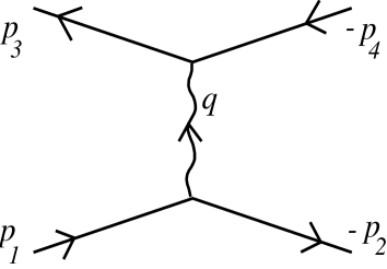
Fig. 1: Leading order contribution to transverse Drell-Yan.

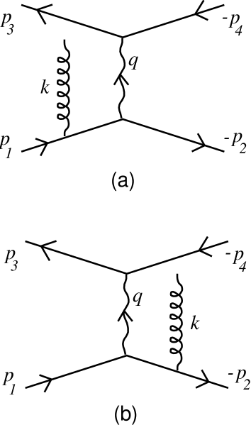
Fig. 2: Bremsstrahlung contributions to transverse Drell-Yan.

References

- [1] S. Kumano and M. Miyama, Phys. Rev. D 56 (1997) 2504.
- [2] W. Vogelsang, Phys. Rev. D 57 (1998) 1886.
- [3] A. Hayashigaki, Y. Kanazawa and Y. Koike, Phys. Rev. D 56 (1997) 7350.
- [4] X. Artru and M. Mekhfi, Z. Phys. C 45 (1990) 669.
- [5] J.P. Ralston and D.E. Soper, Nucl. Phys. B 152 (1979) 109.
- [6] G. ’t Hooft and M. Veltman, Nucl. Phys. B 44 (1972) 189.
- [7] P. Breitenlohner and D. Maison, Commun. Math. Phys. 52 (1977) 11.
- [8] W.J. Marciano and A. Sirlin, Nucl. Phys. B 88 (1975) 86.
- [9] W. Vogelsang and A. Weber, Phys. Rev. D 48 (1993) 2073.
- [10] J. Kubar-André and F.E. Paige, Phys. Rev. D 19 (1979) 221.
- [11] A.P. Contogouris, B. Kamal and Z. Merebashvili, Phys. Lett. B 337 (1994) 169.
- [12] W. Siegel, Phys. Lett. B 84 (1979) 193.
- [13] B. Kamal, Phys. Rev. D 53 (1996) 1142.
- [14] G. Altarelli and G. Parisi, Nucl. Phys. B 126 (1977) 298.
- [15] B. Kamal, Phys. Rev. D 57 (1998) 6663.
- [16] J.G. Korner and M.M. Tung, Z. Phys. C 64 (1994) 255, and references therein.
- [17] W. Siegel, Phys. Lett. B 94 (1980) 37.
- [18] W. Beenakker, H. Kuijf, W.L. van Neerven and J. Smith, Phys. Rev. D 40 (1989) 54.