1 Introduction

It has long been recognized that the strong interaction respects charge symmetry to a high degree. We review the definition of charge symmetry, which is sometimes confused with isospin symmetry. For details we refer the reader to comprehensive reviews on charge symmetry by Miller, Nefkens and Slaus [1], and Henley and Miller [2]. The assumption of isospin independence of hadronic forces requires that the Hamiltonian of the system commutes with the isospin operator T, i.e.

$$\left[H,{\bf T}\right]=\left[H,T^{2}\right]=0$$ (1)

Whereas isospin symmetry requires invariance of the Hamiltonian with respect to all rotations in isospin space, charge symmetry requires invariance only with respect to rotations of $180^{\circ}$ about the $T_{2}$ axis, where the charge corresponds to the third axis in isospin space. Consequently, isospin symmetry necessarily implies the validity of charge symmetry; however, the converse is not necessarily true. As charge symmetry is a more restricted symmetry than isospin symmetry, it is generally conserved in strong interactions to a greater degree than isospin symmetry. Thus, while in many nuclear reactions isospin symmetry is violated at the few percent level, in most cases charge symmetry is obeyed to better than one percent.

For a system of $A$ particles, the charge symmetry operator can be written as

$$P_{cs}=\exp(i\pi T_{2})=\Pi_{i=1}^{A}\exp[i\pi T_{2}(i)]~{}~{}.$$ (2)

The operation of charge symmetry maps up quarks to down, and protons to neutrons. Specifically, under charge symmetry

$$e^{i\pi T_{2}} : u\rightarrow d,p\rightarrow n$$ (3)

$$: d\rightarrow-u,n\rightarrow-p$$

At the quark level, charge symmetry implies the invariance of a system under the interchange of up and down quarks. The proton and neutron each contain three valence quarks, plus a “sea” of quark-antiquark pairs. Coulomb effects aside, the “proton” is converted to a “neutron” by interchanging up and down quarks in the two nucleons. At the level of parton distributions, charge symmetry implies the relations

$$u^{p}(x,Q^{2}) = d^{n}(x,Q^{2})$$

$$d^{p}(x,Q^{2}) = u^{n}(x,Q^{2})$$ (4)

Charge symmetry is broken by electromagnetic interactions, but these should play a minor role at high energies. We can get an estimate for the magnitude of charge symmetry violation [CSV] at the parton level; we would naively expect parton CSV to be of the order of the up–down current quark mass difference divided by some average mass expectation value of the strong Hamiltonian, or $(m_{d}-m_{u})/<M>$, where $<M>$ has a value of roughly 0.5–1.0 GeV. This would naturally put CSV effects at a level of 1% or smaller. Note that we expect charge symmetry to be valid at this level, despite the fact that the current quark masses themselves, i.e. $m_{u}\sim 4$ MeV, $m_{d}\sim 7$ MeV, differ by 50%! However, our understanding is that dynamical chiral symmetry breaking and/or confinement masks this very large “primordial” violation of charge symmetry, and observable quantities are expected to respect charge symmetry to roughly one percent.

In nuclear physics, charge symmetry involves the interchange of protons and neutrons in a system. At low energies, charge symmetry appears to be generally valid at the level of 1% or better in nuclear systems, although there are some notable exceptions to this rule of thumb [1]. The proton and neutron masses are equal to about 0.1%; the binding energies of tritium and ³He are equal to 1%, after Coulomb corrections. We can compare energy levels in “mirror” nuclei (nuclei related to one another by $P_{cs}$), and generally find agreement to better than 1%, after correcting for electromagnetic interactions.

From our experience with charge symmetry in nuclear systems, and because of the order of magnitude estimates of CSV in parton systems, charge symmetry has been universally assumed in quark/parton phenomenology. With this assumption, one reduces the number of independent quark distribution functions by a factor of two. One simply defines all quark distribution functions in the neutron to be equal to the corresponding functions in the proton, while interchanging up and down quarks in the process. The assumption of charge symmetry is sufficiently ingrained in quark/parton phenomenology that its validity is a necessary condition for many relations between structure functions. Thus, it is not apparent to many physicists that several sum rules or structure function equalities may be valid only to the extent that charge symmetry is exact.

Recently, much attention has been focused on the apparent violation of what is called SU(2) flavor symmetry in the nucleon. The measurements of the Gottfried sum rule [3] reported by the New Muon Collaboration (NMC) [4] sparked a great deal of interest in the sea-quark flavor distributions of nucleons [5, 6, 7, 8, 9, 10, 11]. The “natural” explanation of the NMC results is that “SU(2) flavor symmetry” is broken in the proton sea quark distributions (i.e. $\bar{u}^{p}(x)\not=\bar{d}^{p}(x)$). This has been widely cited, and several theoretical investigations have been carried out to investigate the possible origin of this flavor symmetry violation. At the time of the NMC measurements, another possible explanation for this data was that the Gottfried sum rule was obeyed, and that the apparent experimental violation resulted from significant contributions to the sum rule at extremely small values of $x$ [12].

Since the NMC experiment suggested large flavor symmetry violating antiquark distributions, this led people towards experiments which had the possibility of “direct” observation of flavor symmetry violation [FSV] in the proton sea. Ellis and Stirling [13] pointed out that this information could be obtained by studying proton-induced Drell-Yan cross sections with both proton and neutron (i.e., deuteron) targets. Two subsequent experiments have been carried out, by the NA51 group at CERN [14], and the E866 experiment at FNAL [15]. Experimental results from these collaborations also seem to show a large flavor symmetry violation [FSV] in the proton sea quark distributions. We will discuss these results in detail in Sect. 4 of this review.

However, the conclusion that these three experiments demonstrate large FSV effects, as well as the magnitude of the FSV effects extracted, relies on the implicit assumption of charge symmetry. It has been pointed out [16, 17] that all three experimental results (NMC, NA51 and E866) could in principle be explained even if flavor symmetry were conserved, if we assume charge symmetry violation [CSV] in the nucleon sea. As we will show, the CSV terms necessary to account for the results of these experiments would be surprisingly large – much larger than theoretical models would predict. If charge symmetry were violated to this degree in parton distributions, it would be amazing that at low energies it would be nearly an exact symmetry.

However, the history of our understanding of nucleon structure has involved a series of similar “surprises” from experiment: e.g., the significant contribution of antiquarks to nucleon structure functions at small $x$; the large fraction of the nucleon’s momentum carried by glue; the persistence of substantial spin effects at high energies despite perturbative QCD [pQCD] predictions that single-spin asymmetries should vanish; the “spin crisis,” which suggests that a surprisingly small fraction of the proton’s spin may be carried by valence quarks; and the behavior of quark distributions at very small $x$. So, despite the strong indirect evidence from low-energy physics, and straightforward pQCD arguments which suggest that charge symmetry should be valid to about the 1% level in parton distributions, we urge the reader to keep an open mind on this question.

In this paper, we will provide a comprehensive review of the following question: how valid is the assumption of charge symmetry for parton distributions? First, we will redefine the nucleon structure functions in terms of quark/parton distributions, without assuming charge symmetry. Next, we will show how relations between structure functions become modified when we allow CSV terms. We then calculate the CSV contributions to various observables. We examine the current experimental evidence for charge symmetry. As we will show, all experiments to date are consistent with parton charge symmetry. However, in some regions present experimental upper limits on parton charge symmetry violation are rather weak. On the other hand, new experimental neutrino deep inelastic scattering data, when taken together with high energy muon scattering, can provide rather strong constraints on parton CSV, at least for a certain range of Bjorken $x$.

We will also present some simple model estimates of charge symmetry violation in both valence quark and sea quark distributions. For the “majority” valence quark distributions, (i.e., $u^{p}_{\rm v}(x)-d^{n}_{\rm v}(x)$), we predict very small CSV amplitudes, no larger than 1%. However, our model calculation of charge symmetry violation in the “minority” nucleon valence quark distributions ($d^{p}_{\rm v}(x)-u^{n}_{\rm v}(x)$) [18, 19] suggests surprisingly large CSV terms. We discuss several experiments which could detect CSV in parton distributions, or which could improve the current upper limits on quark CSV.

The structure of our paper is as follows. In Sect. 2 we review the general expressions between cross sections and structure functions for deep inelastic scattering processes. We write down the most general form of the structure functions, without assuming charge symmetry. In Sect. 3, we give derivations, from simple models, of charge symmetry breaking for both valence quarks and sea quarks. We show the magnitude and sign of the expected CSV terms in these models. We also review relations between structure functions which hold if charge symmetry is valid.

In Sect. 4 we review those experiments which currently place the best upper limits on CSV in parton distributions. Because of the current interest in flavor symmetry violation in the proton sea, and because current “tests” of FSV in fact are testing a combination of FSV and CSV, we review at length the recent Drell-Yan measurements which are presented as evidence for FSV. We review the constraints which recent experiments place on CSV and FSV in antiquark parton distributions. Preliminary results from the E866 Drell-Yan experiment suggests that they can measure the relative magnitude of $\bar{d}$ and $\bar{u}$ in the proton, over a fairly wide kinematic region. In this same general region, we also have data from the NMC measurement of $F_{2}$ structure functions in protons and neutrons, using high energy muon beams. In addition, we have the structure function $F_{2}^{W^{\pm}}$ measured by the CCFR group, from charge changing weak interactions induced by neutrinos and antineutrinos on iron. All three experiments obtain measurements at similar values of $Q^{2}$ and $x$.

In Sect. 5, we propose experiments which could in principle reveal charge symmetry violation in the valence quark distributions (these would also differentiate between FSV and CSV effects). In Sect. 6, we review QCD sum rules. We show how these are modified if we include sea quark CSV contributions. We review the best known unpolarized sum rules, the Gottfried, Adler and Gross-Llewellyn Smith sum rule. In Sect. 7, we show that by defining two new sum rules, it would be possible to measure separately CSV, and FSV, contributions to sea quark distributions. We call these the “charge symmetry” and “flavor symmetry” sum rules, respectively. We also review the status of existing experiments to determine current upper limits on sea quark CSV via the charge symmetry sum rule. In Sect. 8 we present our conclusions.

2 Relations Between High Energy Cross Sections and Parton Distributions

2.1 General form of high energy cross sections

We can write the cross sections for deep inelastic scattering in terms of a set of structure functions, which depend on the relativistic kinematics of the reaction. Through the quark/parton model, these structure functions can in turn be written in terms of quark/parton distributions [20]. For example, the most general form of the cross section for charged current interactions initiated by charged leptons on nucleons has the form

$${d^{2}\sigma^{l^{+}(l^{-})}_{CC}\over dx\,dy} = {\pi s\over 2}\left({\alpha\over 2\sin^{2}\theta_{W}M_{W}^{2}}\right)^{2}\left({M_{W}^{2}\over M_{W}^{2}+Q^{2}}\right)^{2}\,\left[xy^{2}F_{1}^{W^{\pm}}(x,Q^{2})\right.$$ (5)

$$+ \left.\left(1-y-{xym_{N}^{2}\over s}\right)\,F_{2}^{W^{\pm}}(x,Q^{2})\mp(y-y^{2}/2)xF_{3}^{W^{\pm}}(x,Q^{2})\right]$$

This process is shown schematically in Fig. 1a. It involves a charged virtual $W^{\pm}$ of momentum $q$ being interchanged between the lepton/neutrino vertex, and the hadronic vertex. The relativistic invariants in Eq. 5 are $Q^{2}=-q^{2}$, the square of the four momentum transfer for the reaction, $x$ and $y$. For four momentum $k$ ($p$) for the initial state lepton (nucleon), we have the relations

$$x = {Q^{2}\over 2p\cdot q};\qquad y={p\cdot q\over p\cdot k}$$

$$s = (k+p)^{2}$$ (6)

In Eq. 5, $M_{W}$ is the mass of the charged weak vector boson, and $\theta_{W}$ is the Weinberg angle.

   

Figure 1: Schematic picture of deep inelastic scattering of charged leptons from a nucleon. a) Charged-current weak interactions. An intermediate $W$ is absorbed on the nucleon. b) Neutral-current electroweak interactions.

Similarly, the cross section for charged current interactions initiated by neutrinos or antineutrinos on nucleons has the form

$${d^{2}\sigma^{\nu(\bar{\nu})}_{CC}\over dx\,dy} = \pi s\left({\alpha\over 2\sin^{2}\theta_{W}M_{W}^{2}}\right)^{2}\left({M_{W}^{2}\over M_{W}^{2}+Q^{2}}\right)^{2}\,\left[xy^{2}F_{1}^{W^{\pm}}(x,Q^{2})\right.$$ (7)

$$+ \left.\left(1-y-{xym_{N}^{2}\over s}\right)\,F_{2}^{W^{\pm}}(x,Q^{2})\pm(y-y^{2}/2)xF_{3}^{W^{\pm}}(x,Q^{2})\right]$$

This process is obtained by interchanging the initial and final state leptons in Fig. 1a.

Neutral current (NC) reactions initiated by neutrinos or antineutrinos have the form

$${d^{2}\sigma^{\nu(\bar{\nu})}_{NC}\over dx\,dy} = \pi s\left({\alpha\over 2\sin^{2}\theta_{W}\cos^{2}\theta_{W}M_{Z}^{2}}\right)^{2}\left({M_{Z}^{2}\over M_{Z}^{2}+Q^{2}}\right)^{2}\,\left[xy^{2}F_{1}^{Z}(x,Q^{2})\right.$$ (8)

$$+ \left.\left(1-y-{xym_{N}^{2}\over s}\right)\,F_{2}^{Z}(x,Q^{2})\pm(y-y^{2}/2)xF_{3}^{Z}(x,Q^{2})\right]$$

Finally, the cross section for scattering of a left (L) or right (R) handed charged lepton in NC reactions has the form

$${d^{2}\sigma^{L,R}_{NC}\over dx\,dy} = {4\pi\alpha^{2}s\over Q^{4}}\,\left(\left[xy^{2}F_{1}^{\gamma}(x,Q^{2})+(1-y)F_{2}^{\gamma}(x,Q^{2})\right]\right.$$ (9)

$$- {Q^{2}\over(Q^{2}+M_{Z}^{2})}{v_{\ell}\pm a_{\ell}\over 2\sin\theta_{W}\cos\theta_{W}}\left[xy^{2}F_{1}^{\gamma Z}(x,Q^{2})+(1-y)F_{2}^{\gamma Z}(x,Q^{2})\right.$$

$$\pm \left.(y-y^{2}/2)xF_{3}^{\gamma Z}(x,Q^{2})\right]+\left({Q^{2}\over(Q^{2}+M_{Z}^{2})}\right)^{2}{v_{\ell}\pm a_{\ell}\over 2\sin\theta_{W}\cos\theta_{W}}\left[xy^{2}F_{1}^{Z}(x,Q^{2})\right.$$

$$+ \left.\left.(1-y)F_{2}^{Z}(x,Q^{2})\pm(y-y^{2}/2)xF_{3}^{Z}(x,Q^{2})\right]\right)$$

This process is shown schematically in Fig. 1b. Either a photon or $Z^{0}$ boson can be exchanged in this process.

In Eq. 9, we have

$$v_{e} = {-1+4\sin^{2}\theta_{W}\over 4\sin\theta_{W}\cos\theta_{W}}$$

$$v_{\nu_{e}} = a_{\nu_{e}}=-a_{e}={1\over 4\sin\theta_{W}\cos\theta_{W}}$$ (10)

Eq. 9 describes the deep inelastic scattering for an $L$ ($R$) handed charged lepton from a nucleon. For momentum transfers which are sufficiently small (relative to $M_{Z}^{2}$), we can neglect the contribution from $Z$ bosons, in which case the scattering is a function only of the two electromagnetic structure functions, $F_{1}^{\gamma}$ and $F_{2}^{\gamma}$, respectively.

2.2 Structure functions in terms of quark/parton distributions

The form of the proton structure functions, obtained from deep inelastic scattering of an electron or muon, can be written in terms of interaction of the charged leptons and quarks with the virtual photon $\gamma$ [20]. Here we assume we are at sufficiently low energies that we can neglect contributions from $Z^{0}$ in electroweak processes. From Eq. 9 we see that the resulting cross section can be written in terms of two structure functions, $F_{1}^{\gamma}$ and $F_{2}^{\gamma}$. Furthermore, we work in an energy regime where both $Q^{2}$ and the energy transfer are very large, while $x$ remains finite, so that scaling is valid, i.e. the structure functions (to first approximation) depend only on $x$ and not on $Q^{2}$. The resulting structure function $F_{1}^{\gamma p}(x)$ can be written in terms of the parton distributions as

$$F_{1}^{\gamma p}(x,Q^{2}) \equiv {1\over 2}\left({4\over 9}\,\left[u^{p}(x)+\bar{u}^{p}(x)+c^{p}(x)+\bar{c}^{p}(x)\right]\right.$$ (11)

$$+ \left.{1\over 9}\,\left[d^{p}(x)+\bar{d}^{p}(x)+s^{p}(x)+\bar{s}^{p}(x)\right]\right)$$

This process is shown schematically in Fig. 2. In Eq. 11, we assume we can neglect any contribution from bottom or top quarks in the proton. The virtual photon couples to the squared charge of the struck quarks. To obtain the corresponding $F_{1}$ structure function for the neutron, we simply change the superscript $p\rightarrow n$ everywhere in Eq. 11.

Figure 2: Coupling of a charged lepton to quarks through exchange of a virtual photon.

In Eq. 11 (and in most subsequent equations), we have neglected the dependence of the parton distributions on the scale at which they are evaluated. As is well known [21, 20], there is an uncertainty in the parton distributions with respect to the scale $\mu^{2}$ at which they are evaluated. Once we calculate the parton distributions $q_{k}(x,\mu^{2})$ and gluon distributions at some starting scale, we can evolve the parton distributions to some higher $Q^{2}$ through the QCD evolution equations of Dokshitzer, Gribov, Lipatov, Altarelli and Parisi [22]. For convenience, we will generally omit this scale in equations involving parton distributions.

In the lowest order quark/parton model, the structure function $F_{2}^{\gamma}$ is related to the structure function $F_{1}^{\gamma}$ by the Callan-Gross relation [23]

$$F_{2}^{\gamma}(x,Q^{2})=2xF_{1}^{\gamma}(x,Q^{2})$$

As is well known, the Callan-Gross relation is valid if the virtual photon which initiates this process is completely transverse. The more general relation between the two structure functions is

$$F_{2}^{\gamma}(x,Q^{2})={1+R(x,Q^{2})\over 1+4M^{2}x^{2}/Q^{2}}\,2x\,F_{1}^{\gamma}(x,Q^{2})~{}~{}.$$ (12)

In Eq. 12, $R=\sigma_{L}/\sigma_{T}$ is the ratio of the cross section for longitudinally to transversely polarized photons. An analogous relation will hold for the weak structure functions $F_{i}^{W^{\pm}}$. An empirical relation fit to the world’s available data on $R$ has been made by Whitlow et al. [24]. The formula is

$$R(x,Q^{2}) = {b_{1}\theta\over\ln(Q^{2}/0.04)}+{b_{2}\over Q^{2}}+{b_{3}\over Q^{4}+0.09}~{}~{},$$

$$\theta = 1+{12Q^{2}\over Q^{2}+1}\left({c^{2}\over c^{2}+x^{2}}\right).$$ (13)

The coefficients in Eq. 13 can be found in Ref. [24]. This fit covers the region accessible at that time, i.e. $x>0.1$ and $Q^{2}<125$ GeV².

Charged current neutrino scattering on hadrons is mediated by emission of the weak vector boson $W^{\pm}$ by the leptons and subsequent absorption of the $W^{\pm}$ on the proton or neutron. Thus the structure function $F_{1}$ corresponding to charge-changing interactions of neutrinos on protons can be written in terms of the quark distribution functions as

$$F_{1}^{W^{+}p}(x) \equiv d^{p}(x)|V_{ud}|^{2}+d^{p}(\xi_{c})|V_{cd}|^{2}\theta(x_{c}-x)+\bar{u}^{p}(x)[|V_{ud}|^{2}+|V_{us}|^{2}]$$ (14)

$$+ \bar{u}^{p}(\xi_{b})|V_{ub}|^{2}\theta(x_{b}-x)+s^{p}(x)|V_{us}|^{2}+s^{p}(\xi_{c})|V_{cs}|^{2}\theta(x_{c}-x)$$

$$+ \bar{c}^{p}(\xi_{b})|V_{cb}|^{2}\theta(x_{b}-x)+\bar{c}^{p}(x)[|V_{cd}|^{2}+|V_{cs}|^{2}],$$

In Fig. 3a we show the coupling of the virtual $W^{+}$ to quarks; the coupling is to quarks with negative charge. In Fig. 3b we show the coupling to antiquarks.

     

Figure 3: a) Quark contributions to the charged-current reactions induced by neutrinos. The virtual $W^{+}$ is absorbed by negatively charged quarks. b) Antiquark contributions to neutrino induced charged-current reactions.

Similarly, the structure function $F_{1}$ corresponding to charge-changing reactions for antineutrinos on protons can be written as

$$F_{1}^{W^{-}p}(x) \equiv u^{p}(x)[|V_{ud}|^{2}+|V_{us}|^{2}]+u^{p}(\xi_{b})|V_{ub}|^{2}\theta(x_{b}-x)+\bar{d}^{p}(x)|V_{ud}|^{2}$$ (15)

$$+ \bar{d}^{p}(\xi_{c})|V_{cd}|^{2}\theta(x_{c}-x)+\bar{s}^{p}(x)|V_{us}|^{2}+\bar{s}^{p}(\xi_{c})|V_{cs}|^{2}\theta(x_{c}-x)$$

$$+ c^{p}(\xi_{b})|V_{cb}|^{2}\theta(x_{b}-x)+c^{p}(x)[|V_{cd}|^{2}+|V_{cs}|^{2}].$$

For antineutrinos the virtual $W^{-}$ is absorbed by positively charged quarks and antiquarks. In Eqs. 14 and 15, quantities like $V_{ud}$ are elements of the Cabibbo-Kobayashi-Maskawa (CKM) quark mixing matrix [20]. We have also introduced the so-called “slow rescaling” formalism [25, 26] to account for threshold corrections in heavy quark production. For production of a heavy quark with current quark mass $m_{k}$, we define the quantities

$$\xi_{k}(Q^{2}) = x\left(1+{m_{k}^{2}\over Q^{2}}\right)$$

$$x_{k}(Q^{2}) = {Q^{2}\over Q^{2}+\Delta_{k}^{2}}$$

$$\Delta_{k}^{2} \equiv (M_{X}^{min})^{2}-m_{N}^{2}$$ (16)

In Eq. 16, the quantity $M_{X}^{min}$ is the minimum mass of the final state for the light quark to heavy quark transition. For the various quark flavors, we have $M_{X}^{min}\approx$ 2.8 GeV, 3 GeV, and 6.2 GeV for transitions $d\rightarrow c$, $s\rightarrow c$, and $u\rightarrow b$, respectively (in this review we neglect all contributions from top quarks).

Note that with this rescaling model, the Callan-Gross relation fails to apply in the region of heavy quark thresholds, even in the event that the interactions are purely transverse. The structure function $F_{2}^{W^{+}p}$ can be obtained from $F_{1}^{W^{+}p}$, Eq. 14, by the replacement

$$q_{i}(x)\rightarrow 2xq_{i}(x)\quad\quad q(\xi_{k})\rightarrow 2\xi_{k}q(\xi_{k})~{}~{},$$ (17)

and identical replacements for the antiquark distributions. With the same replacement, Eq. 17, one can obtain the structure function $F_{2}^{W^{-}p}$ from $F_{1}^{W^{-}p}$. Similarly, the structure function ${1\over 2}F_{3}^{W^{\pm}p}$ can be obtained from $F_{1}^{W^{\pm}p}$ by the replacement

$$\bar{q}_{k}(x)\rightarrow-\bar{q}_{k}(x)$$ (18)

2.3 High energy limiting form for weak structure functions

At sufficiently high momentum transfers, e.g. well above charm threshold, we have $\xi_{c}\rightarrow x$. In the limit of very high momentum transfer, $Q^{2}\rightarrow\infty$, we have $\xi_{k}(Q^{2})\rightarrow x$ and $x_{k}\rightarrow 1$ for all heavy quark flavors. In this limit we once again recover the Callan-Gross relation (if $\sigma_{L}/\sigma_{T}\rightarrow 0$). At very high momentum transfers and at very high energy, if we neglect correction terms of magnitude $|V_{ub}|^{2}=|V_{td}|^{2}\approx\sin(\theta_{C})^{6}\approx 1\times 10^{-4}$, then the structure functions $F_{i}^{W^{\pm}}(x,Q^{2})$ reduce to

$$\lim_{Q^{2}\rightarrow\infty}F_{1}^{W^{+}p}(x,Q^{2}) \rightarrow d^{p}(x)+\bar{u}^{p}(x)+s^{p}(x)+\bar{c}^{p}(x)$$

$$F_{1}^{W^{-}p}(x,Q^{2}) \rightarrow u^{p}(x)+\bar{d}^{p}(x)+\bar{s}^{p}(x)+c^{p}(x)$$

$${1\over 2}F_{3}^{W^{+}p}(x,Q^{2}) \rightarrow d^{p}(x)-\bar{u}^{p}(x)+s^{p}(x)-\bar{c}^{p}(x)$$

$${1\over 2}F_{3}^{W^{-}p}(x,Q^{2}) \rightarrow u^{p}(x)-\bar{d}^{p}(x)-\bar{s}^{p}(x)+c^{p}(x),$$ (19)

with the corresponding structure functions for neutrons obtained by replacing superscripts $p\rightarrow n$ everywhere in Eqs. 19. Because of their simplicity we will generally use Eq. 19 in deriving relations between structure functions, although we should revert to Eqs. 14 and 15 when comparing with data. This is particularly relevant for experiments at relatively low $Q^{2}$, where threshold effects can be rather important.

The assumption of charge symmetry for parton distributions is that

$$d^{n}(x) = u^{p}(x)$$

$$u^{n}(x) = d^{p}(x)$$

$$s^{n}(x) = s^{p}(x)=s(x)$$

$$c^{n}(x) = c^{p}(x)=c(x).$$ (20)

We have identical relations for antiquark distributions. With this assumption, all neutron parton distributions can be replaced by the corresponding distributions in the proton. To retain the charge symmetry violating parton distributions, we introduce the CSV parton distributions for up and down quarks via

$$d^{n}(x) \equiv u^{p}(x)-\delta u(x)$$

$$u^{n}(x) \equiv d^{p}(x)-\delta d(x).$$ (21)

If the quantities $\delta u(x)$ and $\delta d(x)$ vanish, then charge symmetry is exact. We have analogous relations for CSV in antiquark distributions. We assume that the strange quark (and antiquark) distributions are the same in both the proton and neutron, as is given in Eq. 20. We make the same assumption for charm quarks. There is no theoretical or experimental reason to expect strange and charm distributions to vary from proton to neutron.

It is useful to divide parton distributions into valence quark and sea quark parts. The valence up quark distribution in the proton is defined by $u^{p}_{\rm v}(x)\equiv u^{p}(x)-\bar{u}^{p}(x)$. The valence quark distributions obey the following quark normalization conditions

$$\int_{0}^{1}\,dx\,u^{p}_{\rm v}(x) = \int_{0}^{1}\,dx\,\left(u^{p}(x)-\bar{u}^{p}(x)\right)=$$

$$\int_{0}^{1}\,dx\,d^{n}_{\rm v}(x) = \int_{0}^{1}\,dx\,\left(d^{n}(x)-\bar{d}^{n}(x)\right)=2;$$

$$\int_{0}^{1}\,dx\,d^{p}_{\rm v}(x) = \int_{0}^{1}\,dx\,\left(d^{p}(x)-\bar{d}^{p}(x)\right)=$$

$$\int_{0}^{1}\,dx\,u^{n}_{\rm v}(x) = \int_{0}^{1}\,dx\,\left(u^{n}(x)-\bar{u}^{n}(x)\right)=1;$$

$$\int_{0}^{1}\,dx\,\left(s(x)-\bar{s}(x)\right) = \int_{0}^{1}\,dx\,\left(c(x)-\bar{c}(x)\right)=0.$$ (22)

The CSV quantities defined in Eq. 21 can have both valence and sea pieces. The valence quark charge symmetry violating distributions are defined as

$$\delta u_{\rm v}(x) = \delta u(x)-\delta\bar{u}(x)$$

$$\delta d_{\rm v}(x) = \delta d(x)-\delta\bar{d}(x)$$ (23)

From these definitions of valence quark CSV, it is straightforward to show that the first moment of the valence quark CSV distributions (i.e., the integral over $x$) must vanish. We see that

$$\int_{0}^{1}dx\delta u_{\rm v}(x) = \int_{0}^{1}dx\left(u^{p}(x)-d^{n}(x)-\bar{u}^{p}(x)+\bar{d}^{n}(x)\right)$$ (24)

$$= \int_{0}^{1}dx\left(u^{p}_{\rm v}(x)-d^{n}_{\rm v}(x)\right)=0$$

In Eq. 24, the integral over the valence quark distributions is fixed by the normalization condition to the number of valence up quarks in the proton (down quarks in the neutron). Since both of these are equal to 2, the integral of $\delta u_{\rm v}(x)$ must give zero.

From Eq. 22 we see that the first moment of the heavy quark and antiquark distributions are identical. Until recently, it was customary to assume that the strange and charmed quark and antiquark distributions were equal for all values of $x$. That is, one assumed that

$$s(x)=\bar{s}(x)\equiv s(x)~{}~{},$$ (25)

with an identical relation for the charmed quark distributions. However, recently there has been both theoretical and experimental interest in whether the strange and antistrange distributions are in fact equal. We will review how strange quark distributions are extracted, and the experimental situation regarding strange and antistrange quark distributions, in Sect. 2.6.

2.4 CSV Contributions to Structure Functions

In the high energy limit, well above heavy quark thresholds, the structure functions for charged current weak interactions on neutrons take the form

$$\lim_{Q^{2}\rightarrow\infty}F_{1}^{W^{+}n}(x,Q^{2}) = d^{n}(x)+\bar{u}^{n}(x)+s(x)+\bar{c}(x)$$

$$F_{1}^{W^{-}n}(x,Q^{2}) = u^{n}(x)+\bar{d}^{n}(x)+\bar{s}(x)+c(x)$$

$${1\over 2}F_{3}^{W^{+}n}(x,Q^{2}) = d^{n}(x)-\bar{u}^{n}(x)+s(x)-\bar{c}(x)$$

$${1\over 2}F_{3}^{W^{-}n}(x,Q^{2}) = u^{n}(x)-\bar{d}^{n}(x)-\bar{s}(x)+c(x).$$ (26)

Introducing the CSV parton distributions from Eq. 21, Eq. 26 becomes

$$\lim_{Q^{2}\rightarrow\infty}F_{1}^{W^{+}n}(x,Q^{2}) = u^{p}(x)+\bar{d}^{p}(x)+s(x)+\bar{c}(x)-\delta u(x)-\delta\bar{d}(x)$$

$$F_{1}^{W^{-}n}(x,Q^{2}) = d^{p}(x)+\bar{u}^{p}(x)+\bar{s}(x)+c(x)-\delta d(x)-\delta\bar{u}(x)$$

$${1\over 2}F_{3}^{W^{+}n}(x,Q^{2}) = u^{p}(x)-\bar{d}^{p}(x)+s(x)-\bar{c}(x)-\delta u(x)+\delta\bar{d}(x)$$

$${1\over 2}F_{3}^{W^{-}n}(x,Q^{2}) = d^{p}(x)-\bar{u}^{p}(x)-\bar{s}(x)+c(x)-\delta d(x)+\delta\bar{u}(x).$$ (27)

For completeness, we include the electromagnetic structure function for neutron targets. Eq. 11 becomes

$$F_{1}^{\gamma n}(x,Q^{2}) = {1\over 2}\left({4\over 9}\,\left[u^{n}(x)+\bar{u}^{n}(x)+c(x)+\bar{c}(x)\right]+{1\over 9}\,\left[d^{n}(x)+\bar{d}^{n}(x)+s(x)+\bar{s}(x)\right]\right)$$ (28)

$$= {1\over 2}\left({4\over 9}\,\left[d^{p}(x)+\bar{d}^{p}(x)+c(x)+\bar{c}(x)\right]+{1\over 9}\,\left[u^{p}(x)+\bar{u}^{p}(x)+s(x)+\bar{s}(x)\right]\right.$$

$$- \left.{4\over 9}\,\left[\delta d(x)+\delta\bar{d}(x)\right]-{1\over 9}\,\left[\delta u(x)+\delta\bar{u}(x)\right]\right).$$

Many tests of charge symmetry will involve deep inelastic scattering on isoscalar targets, which we label as $N_{0}$. Such reactions involve equal contributions from protons and neutrons. Under the assumptions we have listed previously, the weak and electromagnetic structure functions on isoscalar targets can be written (in terms of structure functions per nucleon)

$$F_{1}^{W^{+}N_{0}}(x,Q^{2}) = {1\over 2}\left(u^{p}(x)+d^{p}(x)+\bar{u}^{p}(x)+\bar{d}^{p}(x)+2s(x)+2\bar{c}(x)-\delta u(x)-\delta\bar{d}(x)\right)$$

$$F_{1}^{W^{-}N_{0}}(x,Q^{2}) = {1\over 2}\left(u^{p}(x)+d^{p}(x)+\bar{u}^{p}(x)+\bar{d}^{p}(x)+2\bar{s}(x)+2c(x)-\delta d(x)-\delta\bar{u}(x)\right)$$

$${1\over 2}F_{3}^{W^{+}N_{0}}(x,Q^{2}) = {1\over 2}\left(u^{p}(x)+d^{p}(x)-\bar{u}^{p}(x)-\bar{d}^{p}(x)+2s(x)-2\bar{c}(x)-\delta u(x)+\delta\bar{d}(x)\right)$$

$${1\over 2}F_{3}^{W^{-}N_{0}}(x,Q^{2}) = {1\over 2}\left(u^{p}(x)+d^{p}(x)-\bar{u}^{p}(x)-\bar{d}^{p}(x)-2\bar{s}(x)+2c(x)-\delta d(x)+\delta\bar{u}(x)\right)~{}~{},$$

$$F_{1}^{\gamma N_{0}}(x,Q^{2}) = {1\over 4}\left({5\over 9}\,\left[u^{p}(x)+d^{p}(x)+\bar{u}^{p}(x)+\bar{d}^{p}(x)\right]+{2\over 9}\,\left[s(x)+\bar{s}(x)\right]\right.$$ (29)

$$+ \left.{8\over 9}\,\left[c(x)+\bar{c}(x)\right]-{4\over 9}\,\left[\delta d(x)+\delta\bar{d}(x)\right]-{1\over 9}\,\left[\delta u(x)+\delta\bar{u}(x)\right]\right)$$

2.5 Isolating CSV Effects in Structure Functions

In order to isolate and measure CSV effects, we need to find relations between various structure functions which depend on the validity of charge symmetry, and which can be tested. There are two such relations: the relation between the $F_{1}$ (or $F_{2}$) charge-changing electroweak structure functions from neutrino and antineutrino reactions, and the relation between the $F_{2}$ structure functions obtained from neutrino deep inelastic scattering, and the $F_{2}$ structure function from deep inelastic scattering induced by charged leptons (muons or electrons).

We first discuss the $F_{1}$ structure functions for charge-changing weak interactions. For deep inelastic scattering on an isoscalar target, we can derive the following identity from Eq. 29:

$$\lim_{Q^{2}\rightarrow\infty}\left(F_{1}^{W^{+}N_{0}}(x,Q^{2})-F_{1}^{W^{-}N_{0}}(x,Q^{2})\right) = {1\over 2}\left(\delta d_{\rm v}(x)-\delta u_{\rm v}(x)\right)$$

$$+ s(x)-\bar{s}(x)-c(x)+\bar{c}(x)$$

$${CS\atop=} \,s(x)-\bar{s}(x)-c(x)+\bar{c}(x)$$ (30)

For Eq. 30 to be valid, we must be at sufficiently high values of $Q^{2}$ that we are well above both charm and bottom thresholds. Furthermore, we neglect terms of order $|V_{ub}|^{2}=|V_{td}|^{2}\approx 1\times 10^{-4}$. Eq. 30 should be true at all values of $x$. The final line of this equation holds in the limit that charge symmetry is exact. To avoid confusion in this review, we have introduced the notation ${CS\atop=}$. This means that an equation is true provided charge symmetry is exact. In this way we hope one can distinguish between relations which are generally true, and those which require the (generally implicit) assumption of charge symmetry.

At sufficiently high energies (well above heavy quark production thresholds) threshold effects should become negligible, and then Eq. 30 should be valid. If these structure functions are not equal at all values of $x$, this implies either charge symmetry violation in parton distributions, or inequality of the strange quark and antiquark distributions (the charm quark contributions should be quite small, and we know of no theoretical reason why charm and anticharm distributions should be unequal). In Sect. 5.1 we present theoretical estimates of valence quark CSV and strange/antistrange quark contributions to this relation.

From Eqs. 19 and 27 we can also derive relations between the $F_{1}$ structure functions for neutrinos on protons, and antineutrinos on neutrons,

$$F_{1}^{W^{+}p}(x,Q^{2})-F_{1}^{W^{-}n}(x,Q^{2}) = \delta d(x)+\delta\bar{u}(x)+s(x)-\bar{s}(x)-c(x)+\bar{c}(x)$$

$$F_{1}^{W^{+}n}(x,Q^{2})-F_{1}^{W^{-}p}(x,Q^{2}) = -\delta u(x)-\delta\bar{d}(x)+s(x)-\bar{s}(x)-c(x)+\bar{c}(x).$$ (31)

Eqs. 31 are valid under the same conditions as Eq. 30, namely that we are well above heavy quark thresholds, and that we neglect Kobayashi-Maskawa matrix elements of order $10^{-4}$. If parton charge symmetry were exact, and strange quark and antiquark parton distributions are identical at all $x$, then we would expect

$$F_{1}^{W^{+}p}(x,Q^{2})\, = \,F_{1}^{W^{-}n}(x,Q^{2})$$

$$F_{1}^{W^{-}p}(x,Q^{2})\, = \,F_{1}^{W^{+}n}(x,Q^{2})$$ (32)

At sufficiently high energies, if charge symmetry is valid for valence quark distributions, and if the strange quark and antiquark distributions are equal at all $x$, then the $F_{1}^{W^{\pm}}$ structure functions are identical for isoscalar nuclear targets. Identical relations hold for the $F_{2}$ structure functions, when we include the longitudinal/transverse ratio $R$ of Eq. 13. These equations have been used to extract the structure functions $F_{3}$ in electroweak reactions. Using Eqs. 32 and 7, we can derive

$${3\pi\over 2G^{2}M_{N}E}\left(d\sigma^{\nu p}/dx-d\sigma^{\bar{\nu}n}/dx\right) = F_{2}^{W^{+}p}(x,Q^{2})-F_{2}^{W^{-}n}(x,Q^{2})$$

$$+ {1\over 2}\left(xF_{3}^{W^{+}p}(x,Q^{2})+xF_{3}^{W^{-}n}(x,Q^{2})\right)$$

$${CS\atop=} \ {1\over 2}\left(xF_{3}^{W^{+}p}(x,Q^{2})+xF_{3}^{W^{-}n}(x,Q^{2})\right)$$

$${3\pi\over 2G^{2}M_{N}E}\left(d\sigma^{\nu n}/dx-d\sigma^{\bar{\nu}p}/dx\right) = F_{2}^{W^{+}n}(x,Q^{2})-F_{2}^{W^{-}p}(x,Q^{2})$$

$$+ {1\over 2}\left(xF_{3}^{W^{+}n}(x,Q^{2})+xF_{3}^{W^{-}p}(x,Q^{2})\right)$$

$${CS\atop=} \ {1\over 2}\left(xF_{3}^{W^{+}n}(x,Q^{2})+xF_{3}^{W^{-}p}(x,Q^{2})\right)$$

$${3\pi\over 2G^{2}M_{N}E}\left(d\sigma^{\nu N_{0}}/dx-d\sigma^{\bar{\nu}N_{0}}/dx\right) = F_{2}^{W^{+}N_{0}}(x,Q^{2})-F_{2}^{W^{-}N_{0}}(x,Q^{2})$$ (33)

$$+ {1\over 2}\left(xF_{3}^{W^{+}N_{0}}(x,Q^{2})+xF_{3}^{W^{-}N_{0}}(x,Q^{2})\right)$$

$${CS\atop=} \ {1\over 2}\left(xF_{3}^{W^{+}N_{0}}(x,Q^{2})+xF_{3}^{W^{-}N_{0}}(x,Q^{2})\right),$$

where in Eq. 33 we define

$$d\sigma^{\nu p}(x,Q^{2})/dx = \int_{0}^{1}dy\,d^{2}\sigma^{\nu p}(x,y)/dx\,dy$$

$$G^{2} = {(\pi\alpha)^{2}\over 2M_{W}^{4}\sin^{4}\theta_{W}}$$ (34)

From Eqs. 31 and 33, we see that if charge symmetry is exact, and if the strange quark and antiquark distributions are equal at all $x$, then by taking the difference between cross sections for the appropriate charged current cross sections for neutrinos and antineutrinos, the relevant $F_{2}$ structure functions will cancel, leaving just the $F_{3}$ structure functions. This follows from Eq. 32. In particular, the difference between the charged current cross section from neutrino scattering on an isoscalar target, and the cross section from antineutrinos on that target, is just equal to the sum of the structure functions $xF_{3}$ for neutrinos and antineutrinos on the isoscalar target.

If we don’t require charge symmetry and equality of strange and antistrange quark distributions, then Eq. 33 becomes

$${3\pi\over 2G^{2}M_{N}E}\left(d\sigma^{\nu p}/dx-d\sigma^{\bar{\nu}n}/dx\right) = 2x\left[\delta d(x)+\delta\bar{u}(x)+s(x)-\bar{s}(x)\right]$$

$$+ {1\over 2}\left(xF_{3}^{W^{+}p}(x,Q^{2})+xF_{3}^{W^{-}n}(x,Q^{2})\right)$$

$${3\pi\over 2G^{2}M_{N}E}\left(d\sigma^{\nu n}/dx-d\sigma^{\bar{\nu}p}/dx\right) = 2x\left[-\delta u(x)-\delta\bar{d}(x)+s(x)-\bar{s}(x)\right]$$

$$+ {1\over 2}\left(xF_{3}^{W^{+}n}(x,Q^{2})+xF_{3}^{W^{-}p}(x,Q^{2})\right)$$

$${3\pi\over 2G^{2}M_{N}E}\left(d\sigma^{\nu N_{0}}/dx-d\sigma^{\bar{\nu}N_{0}}/dx\right) = x\left[\delta d_{\rm v}(x)-\delta u_{\rm v}(x)+2\left(s(x)-\bar{s}(x)\right)\right]$$ (35)

$$+ {1\over 2}\left(xF_{3}^{W^{+}N_{0}}(x,Q^{2})+xF_{3}^{W^{-}N_{0}}(x,Q^{2})\right),$$

There are additional terms arising from charm quark distributions; they are given in Eq. 31, but we have not included them in Eq. 35.

From Eq. 35 we see that the difference between neutrino and antineutrino cross sections on an isoscalar target contains not only the $F_{3}$ structure functions, but two residual terms – one of which depends on the quark CSV amplitudes, and the other depending on the difference between strange and antistrange quark distributions. These additional terms then make a contribution at various $x$ values to the sum of the $F_{3}$ structure functions on isoscalar targets. From Eq. 29, without these additional terms the difference between charge-changing reactions induced by neutrinos and antineutrinos gives the sum of up plus down valence quark distributions in the nucleon.

The other relation between structure functions which allows an experimental test of charge symmetry is the so-called “charge ratio” or the “5/18^th rule.” Neglecting for the moment the longitudinal/transverse ratio $R$ (which will cancel if we form the ratio of the two structure functions), we have from Eq. 29

$$\overline{F_{2}}^{W\,N_{0}}(x,Q^{2}) \equiv {F_{2}^{W^{+}\,N_{0}}(x,Q^{2})+F_{2}^{W^{-}\,N_{0}}(x,Q^{2})\over 2}=x\left[\overline{Q}(x)\right.$$

$$- \left.{1\over 2}\left(\delta u(x)+\delta\bar{u}(x)+\delta d(x)+\delta\bar{d}(x)\right)\right],$$

$$F_{2}^{\gamma\,N_{0}}(x,Q^{2}) = x\left[{5\over 18}\overline{Q}(x)-{1\over 6}\left(s(x)+\bar{s}(x)-c(x)-\bar{c}(x)\right)\right.$$

$$- \left.{2\over 9}\left(\delta d(x)+\delta\bar{d}(x)\right)-{1\over 18}\left(\delta u(x)+\delta\bar{u}(x)\right)\right]~{}~{},$$

$$\overline{Q}(x) \equiv \sum_{j=u,d,s,c}q_{j}(x)+\bar{q}_{j}(x)$$ (36)

From Eq. 36, if we take the ratio of the two $F_{2}$ structure functions we obtain

$${F_{2}^{\gamma\,N_{0}}(x,Q^{2})\over\overline{F_{2}}^{W\,N_{0}}(x,Q^{2})} = {5\over 18}\left[1-{3\left(s(x)+\bar{s}(x)\right)\over 5\overline{Q}(x)}-{4\delta d(x)+4\delta\bar{d}(x)+\delta u(x)+\delta\bar{u}(x)\over 5\overline{Q}(x)}\right]$$

$$/ \left[1-{\delta d(x)+\delta\bar{d}(x)+\delta u(x)+\delta\bar{u}(x)\over 2\overline{Q}(x)}\right]~{}~{},$$

$$\approx {5\over 18}\left[1-{3\left(s(x)+\bar{s}(x)\right)\over 5\overline{Q}(x)}+{3\left(\delta u(x)+\delta\bar{u}(x)-\delta d(x)-\delta\bar{d}(x)\right)\over 10\overline{Q}(x)}\right]$$

$${CS\atop=} \,{5\over 18}\left[1-{3\left(s(x)+\bar{s}(x)\right)\over 5\overline{Q}(x)}\right]$$

In Eq. LABEL:Rcdef we have dropped the small contribution from charm quarks. In the second of Eqs. LABEL:Rcdef we have expanded to lowest order in the (small) CSV terms. The ratio $5/18$ in Eq. LABEL:Rcdef, the so-called “charge ratio” for these structure functions, occurs because the virtual photon couples to the squared charge of the quarks, while the charged-current reactions induced by neutrinos couple to the weak isospin mediated by $W$ exchange.

In the charge symmetric limit, we can use the $F_{2}$ structure functions from either neutrino or antineutrino induced reactions, since

$$F_{2}^{W^{+}\,N_{0}}(x,Q^{2}) {CS\atop=} F_{2}^{W^{-}\,N_{0}}(x,Q^{2}){CS\atop=}\overline{F_{2}}^{W\,N_{0}}(x,Q^{2}).$$

If we use the neutrino or antineutrino $F_{2}$ structure functions instead of their average in Eq. LABEL:Rcdef, the only thing which changes in the ratio is the weighting of the various CSV terms, plus an additional contribution if the strange and antistrange distributions are not identical.

In order to get theoretical estimates for the structure function relations, we need to know the quark CSV contributions, and we also need to know the strange quark and antiquark distributions in the nucleon. The strange quark and antiquark distributions can be obtained experimentally by measuring production of opposite sign dimuons in reactions induced by neutrinos or antineutrinos. We review this in the following section. We obtain estimates for the charge-symmetry violating parton distributions using the model for quark CSV which we derive in Sect. 3. In Sect. 4, we will estimate the contribution of the CSV terms to existing tests of charge symmetry at high energies. In Sect. 6, we will discuss possible CSV sea quark contributions to the various sum rules, in particular the Adler and Gross-Llewellyn Smith sum rules.

2.6 Extraction of Strange Quark Distributions

In Sect. 2.3 we introduced the assumption that strange quark and antiquark distributions were identical at all $x$, and were identical for protons and neutrons (a similar assumption is made for charmed quark distributions). In Sect. 2.5 we saw that structure function tests of charge symmetry also contained contributions from strange quark and antiquark distributions. Thus, to get accurate tests of parton charge symmetry, we must have reliable measurements of strange quark distributions.

The strange quark distribution can be assessed in two ways. First, it can be obtained “indirectly” by comparing DIS reactions induced by charged leptons (muons or electrons) with charge-changing currents from neutrinos. From Eq. 36, we see that for an isoscalar target (assuming the Callan-Gross relation and neglecting charm quark contributions), we have

$$\overline{F_{2}}^{W\,N_{0}}(x,Q^{2})-{18\over 5}F_{2}^{\gamma N_{0}}(x,Q^{2}) = {3x\over 10}\left[\delta u(x)+\delta\bar{u}(x)-\delta d(x)-\delta\bar{d}(x)\right]$$ (38)

$$+ {3x\over 5}\left[s(x)+\bar{s}(x)\right]$$

Eq. 38 is “indirect”, in that we must compare experiments with muon and neutrino beams, performed under different conditions and with different normalizations. Furthermore, we need to know the CSV contributions in order to extract the strange quark distribution.

The “direct” way of extracting strange quark distributions is by measuring the yield of opposite sign dimuons produced in nuclear reactions induced by neutrinos. In leading order, the incoming neutrino has a hard scattering with an $s$ or $d$ quark, producing a charm quark which fragments into a charmed hadron. The subsequent semileptonic decay of the charmed hadron produces an opposite sign muon, through the process

$$\nu_{\mu}+N\rightarrow\mu^{-} + c+X$$

$$\rightarrow \mu^{+}+\nu_{\mu}$$

The antineutrino process produces charm antiquarks from $\bar{d}$ and $\bar{s}$ sea quarks. As the first muon produced tends to come from the original scattering and to have larger transverse momentum with respect to the direction of the hadron shower, experimenters can tell whether the muon pair arose from a neutrino or antineutrino collision. In this section we summarize the latest direct measurements and their results.

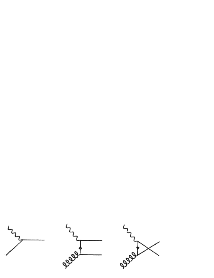
Figure 4: Contribution to production of an opposite sign dimuon pair via intermediate charm quark production. Leading-order quark initiated diagram, plus two NLO gluon-initiated diagrams.

In Fig. 4 we show the leading order [LO] mechanism for production of $\mu^{+}\mu^{-}$ pairs in neutrino-induced reactions. A virtual $W^{+}$ is absorbed on an $s$ or $d$ quark, producing a charm quark, which then decays semi-leptonically. Using the slow rescaling model [25] and assuming charge symmetry, the leading order cross section for production of opposite sign dimuons, for neutrino reactions on an isoscalar target, has the form

$${d^{2}\sigma(\nu N_{0}\rightarrow\mu^{+}\mu^{-}X)\over d\xi_{c}dy} = {G^{2}ME_{\nu}\over\pi}\left[\left(\xi_{c}u(\xi_{c},\mu^{2})+\xi_{c}d(\xi_{c},\mu^{2})\right)|V_{cd}|^{2}+2\xi_{c}s(\xi_{c},\mu^{2})|V_{cs}|^{2}\right]$$ (39)

$$\times \left[1-{m_{c}^{2}\over 2ME_{\nu}\xi_{c}}\right]D(z)B_{c}$$

In Eq. 39, $D(z)$ is the fragmentation function for a charmed quark into a charmed hadron, and $B_{c}$ is the branching ratio for semileptonic decay of a charmed hadron. The quantity $\xi_{c}$ is given by the slow rescaling formula, Eq. 16, and the parton distributions depend through QCD on the scale $\mu^{2}$. The corresponding cross sections for antineutrino interactions are obtained by replacing $q_{k}(\xi_{c},\mu^{2})$ by $\bar{q}_{k}(\xi_{c},\mu^{2})$ for each quark flavor, in Eq. 39.

Because the CKM matrix element $V_{cs}$ is substantially larger than $V_{cd}$, i.e. $|V_{cs}|^{2}\approx 0.95$ while $|V_{cd}|^{2}\approx 0.05$, opposite sign dimuon production from neutrinos is most sensitive to the strange quark distribution in the nucleon, even though the $d$ quark content of the proton is roughly ten times the strange quark density. So the Cabibbo suppression of the $d$ quark contribution to charm production makes the strange quark contribution relatively more important. This suppression factor is also present for reactions induced by antineutrinos, but here the relevant antiquark distributions $\bar{s}$ and $\bar{d}$ are equal to within about a factor of two.

Because of the suppression of contributions from the valence quarks, the next-to-leading [NLO] contributions from gluon exchange turn out to be quite important [27]. The most important such processes, $t$ and $u$ channel diagrams initiated by gluons, are also shown in Fig. 4 . The extra factor of $\alpha_{s}$ which enters these diagrams is compensated for by the fact that the gluon density is an order of magnitude larger than the antiquark density. It turns out to be crucial to include the NLO contributions to this reaction, in this kinematic region (relatively near charm threshold).

Recent measurements by the CCFR collaboration (experiments E744 and E770 at the Fermilab Tevatron with the quadrupole triplet neutrino beam) [28, 29, 21] have amassed a substantial number of events for both neutrinos and antineutrinos. The following results have been obtained with the latest NLO analysis of the CCFR data [30]. In Fig. 5a we plot $x\bar{q}(x,\mu^{2})=x\bar{u}(x,\mu^{2})+x\bar{d}(x,\mu^{2})+xs(x,\mu^{2})$ extracted from these measurements [30], for a scale $\mu^{2}=4$ GeV². In Fig. 5b we plot the strange quark distribution $xs(x,\mu^{2})$ at the same scale. Both the LO results, and the NLO results, are plotted. We see that the NLO curves differ dramatically from the LO results, with the NLO curves much softer than the LO results (they are significantly larger at small $x$ and fall off faster) .

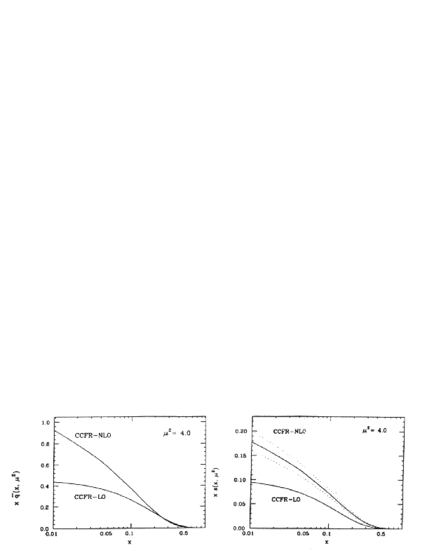
Figure 5: a) Sea quark distribution $x\sum_{j}\bar{q}_{j}(x)(x)$, $j=u,d,s$, from NLO analysis of CCFR Collaboration data, Ref. [30]. b) Strange quark distribution $s(x)$ from same data.

Second, the strange/nonstrange antiquark fraction can be extracted. If we define

$$\kappa = {S+\bar{S}\over(\bar{U}+\bar{D})},\quad{\rm where}$$

$$S = \int_{0}^{1}xs(x)dx,\quad{\rm the~{}CCFR~{}group~{}obtain}$$

$$\kappa = 0.477{+0.046\atop-0.044}{\rm(stat)}+{+0.023\atop-0.024}{\rm(syst)}$$ (40)

The extracted value of $\kappa$ shows a substantial violation of SU(3) symmetry in the nucleon sea. However, the value of $\kappa$ obtained in the NLO analysis [21] is substantially larger than the result obtained in a LO analysis of the same data [29], which produced a value $\kappa_{LO}\approx 0.37$. This arises because the CCFR structure functions extracted from the NLO analysis give larger values at small $x$ for both the nonstrange sea and the strange sea. The importance of the NLO analysis is quite striking here.

Next, the CCFR group compared the $x$ dependence of the strange and nonstrange sea. They parameterized the strange quark distribution as

$$xs(x,\mu^{2})=A_{s}(1-x)^{\alpha}\left[{x\bar{u}(x,\mu^{2})+x\bar{d}(x,\mu^{2})\over 2}\right]$$ (41)

They obtained the best fit value $\alpha=-0.02+{+0.60\atop-0.54}{\rm(stat)}+{+0.28\atop-0.26}$ (syst). This value is consistent with zero, so the $x$ dependence of strange and nonstrange sea appears to be identical. The LO analysis [29] appeared to show a much softer $s$ distribution than the nonstrange sea.

Fourth, this data can be used to extract the CKM matrix element $V_{cd}$. At present, the uncertainty in this parameter gives the greatest contribution to the uncertainty in the Weinberg angle, $\sin^{2}(\theta_{W})$.

Finally, the CCFR group tested whether the strange antiquark distribution $\bar{s}(x)$ differed in shape from the strange quark distribution $s(x)$. The LO analysis of this group [29] had suggested some difference between the two distributions. There have been several theoretical suggestions that this might be the case [32, 33, 34, 35, 36]. If this should prove to be the case, then our formulae for CSV need to be modified to include differences between quark and antiquark distributions for heavy quark flavors. This will turn out to be particularly important in tests of charge symmetry involving charge-changing weak currents on isoscalar nuclei, as is discussed in Sect. 5.1.

The CCFR group analyzed their strange quark distributions assuming that $xs(x,\mu^{2})=(1-x)^{\beta}x\bar{s}(x,\mu^{2})$. They obtained the value $\beta=-0.46\pm 0.42\pm 0.36\pm 0.65\pm 0.17$; the quoted errors (from left to right) are statistical, systematic, from the uncertainty in the semileptonic charged hadron branching ratios, and the uncertainty in $\mu^{2}$ scale. The value obtained is consistent with zero, i.e. no difference in the shape of the strange and antistrange distributions.

Let us review the outline for subsequent sections of this paper. In Sect. 3, we review model calculations which give order of magnitude estimates for charge symmetry violating contributions to both valence and sea quark distributions. In Sect. 4 we review existing experiments which allow us to put upper limits on the magnitude of charge symmetry violation in the parton distributions. We will show that present upper limits on CSV in parton distributions depend on the $x$ region in question. In the region $0.1\leq x\leq 0.4$, the comparison of CCFR neutrino structure functions to the structure functions from the NMC muon measurements suggests an upper limit on CSV of a few percent. At larger values of $x$, there is much less experimental data, so the upper limits on parton CSV are at least 10% in the parton distributions. For smaller values $0.01\leq x\leq 0.1$, the NMC and CCFR results currently disagree at a level between $10-20$%.

We will also review recent experimental tests of flavor symmetry in the proton sea. We will show that these “tests” demonstrate large breaking of either flavor symmetry or charge symmetry, and that at the present time it is difficult to rule out significant breaking of charge symmetry in the nucleon sea (although we certainly do not expect CSV effects of the magnitude necessary to agree with recent Drell-Yan experiments). In Sect. 5 we suggest several new experiments which can differentiate between charge symmetry and flavor symmetry. These experiments, if carried out, could either demonstrate the existence of CSV terms in parton distributions, or provide more stringent upper limits on quark CSV.

3 Theoretical Estimates of Charge Symmetry Violation in Parton Distributions

In this section, we will derive theoretical estimates for charge symmetry violation in parton distributions. First, we will review theoretical calculations of CSV for valence quark distributions. Next, we will give an estimate of the size of CSV effects in antiquark distributions. We will discuss the robustness of these estimates. In later sections, these calculations will be used to provide estimates of the magnitude of CSV effects which could be expected in various experiments. In absence of more detailed calculations of CSV effects, and lacking firm upper limits from experiment, these estimates are the best we have at present. As we will show, we believe that our estimates of both the sign and magnitude of valence quark CSV effects should be rather well determined. Neither the sign nor magnitude of sea quark CSV contributions is well known; however, our model calculations predict very small CSV effects from the sea.

3.1 Charge Symmetry Violation for Valence Quarks

Theoretical investigations of parton CSV for valence quark distributions by Sather [18], Rodionov, Thomas and Londergan [19] and Benesh and Goldman [37] concluded that one could make reasonably model-independent estimates of the size of these effects. Here we follow the method for calculating twist-two parton distributions with proper support, which has been developed by the Adelaide group [38, 39, 40]. The starting point is the evaluation of quark distributions through the relation

$$q(x,\mu^{2})=M\sum_{X}\,|<X|\psi_{+}(0)|N>|^{2}\,\delta(M(1-x)-p_{X}^{+})$$ (42)

In Eq. 42, $\psi_{+}=(1+\alpha_{3})\psi/2$, $X$ represents a complete set of eigenstates of the Hamiltonian, and $\mu^{2}$ represents the starting scale for the quark distribution.

The advantage of this method is that the resulting parton distribution $q(x,\mu^{2})$ is guaranteed to have proper support, i.e. it vanishes for $x>1$, regardless of the model used for the matrix element $<X|\psi_{+}(0)|N>$ in Eq. 42. Parton distributions calculated from quark models generally lack this support, and this can lead to serious problems in obtaining reliable results. Thus, Thomas and collaborators showed that reasonable parton distributions could be obtained from models such as the MIT bag [38]. The other advantage of this method is that it is often possible to obtain reasonable results taking into account only the lowest-energy spectator states in the sum over states of Eq. 42.

We want to use the relation in Eq. 42 to calculate differences in parton distributions due to violation of charge symmetry. Thus, we wish to estimate the difference between, say, the up quark distribution in the proton and the down quark distribution in the neutron. From Eq. 42 we see that CSV contributions will have four sources: first, from electromagnetic effects which break charge symmetry; second, from charge symmetry violating mass differences of the struck quark; third, from mass differences in the spectator multiquark system; and fourth from charge symmetry violation in the quark wavefunctions. In model calculations, it was found that the quark wavefunctions are almost invariant under small mass changes typical of CSV. At high energies, electromagnetic effects should also be small, and we neglect these. Consequently, parton charge symmetry violation will arise predominantly through mass differences of the struck quark, and from mass differences in the spectator multiquark system.

As an example, we consider valence quark CSV where for the intermediate states $X$ in Eq. 42 we include the lowest two-quark spectator states from the MIT bag model [19, 41, 38, 39]. There are more sophisticated quark models available but the similarity of the results obtained by Naar and Birse [42] using the color dielectric model suggests that similar results would be obtained in any relativistic model based on confined current quarks. In Fig. 6 we show schematically the lowest contributions to the “majority valence quark” distributions, i.e. $u^{p}_{\rm v}(x)$ and $d^{n}_{\rm v}(x)$. The majority quark CSV term is as defined in Eq. 23, $\delta u_{\rm v}(x)=u_{\rm v}^{p}(x)-d_{\rm v}^{n}(x)$. From Fig. 6 we see that the only contribution to the “majority” quark CSV is the up-down mass difference $m_{u}-m_{d}$; the intermediate spectator diquark is the same ($ud$) for both proton and neutron.

   

Figure 6: Schematic picture of lowest energy contributions to “majority” quark distributions: struck quark plus spectator diquark. (a) $u^{p}(x)$ for proton. (b) $d^{n}(x)$ for neutron.

   

Figure 7: Schematic picture of lowest energy contributions to “minority” quark distributions. (a) $d^{p}(x)$ for proton. (b) $u^{n}(x)$ for neutron.

In Fig. 7 we show the lowest contributions to the “minority valence quark” distributions, i.e. $d^{p}_{\rm v}(x)$ and $u^{n}_{\rm v}(x)$. From Fig. 7 we see that there are two contributions to minority quark CSV. One is the up-down mass difference $m_{u}-m_{d}$; the second source of charge symmetry violation comes from the intermediate spectator diquark mass, which is $uu$ for the proton and $dd$ for the neutron. In Fig. 8 we show the calculated minority valence quark CSV term, $\delta d_{\rm v}(x)=d^{p}_{\rm v}(x)-u^{n}_{\rm v}(x)$. Fig. 9 shows the majority valence quark CSV term, $\delta u_{\rm v}(x)=u^{p}_{\rm v}(x)-d^{n}_{\rm v}(x)$. These are calculated from Eq. 42 using quark wave functions from the MIT bag model. The contributions are calculated at the bag scale, then evolved upwards in $Q^{2}$. At small $x$, $\delta d_{\rm v}(x)$ is negative, while for larger $x$ it is positive. The majority quark CSV term has exactly the opposite sign. As a result, theoretical calculations suggest that

$$|\delta u_{\rm v}(x)+\delta d_{\rm v}(x)|<<|\delta u_{\rm v}(x)-\delta d_{\rm v}(x)|~{}~{},$$ (43)

so that experimental quantities which depend on the sum of the majority and minority valence quark CSV terms should be substantially smaller than those which depend on the difference between the majority and minority CSV terms.

Figure 8: Calculation of minority valence quark CSV contribution, $\delta d_{v}(x)$ vs. $x$. Dotted curve: $Q^{2}=10$ GeV²; dashed curve: $Q^{2}=100$ GeV²; dot-dashed curve: $Q^{2}=400$ GeV²; dash-triple dot curve: $Q^{2}=10,000$ GeV². From Ref. [74].

Figure 9: Majority valence quark CSV contribution, $\delta u_{v}(x)$. Notation is that of Fig. 8.

Because the integral over $x$ of the valence quark distributions is normalized (one for the minority valence quark distribution, two for the majority distribution), the integral of the CSV distributions must be zero, i.e.

$$\int_{0}^{1}\delta u_{\rm v}(x)\,dx=\int_{0}^{1}\delta d_{\rm v}(x)\,dx=0$$ (44)

In Fig. 10 we show the percent CSV contribution, $\delta d_{\rm v}(x)/d_{\rm v}^{p}(x)$ vs. $x$. For large $x$, i.e. $x\geq 0.5$, the minority valence quark CSV is predicted to be between $5-10$%. This is an extremely large violation of charge symmetry, especially since at low energy scales (e.g., low energy nuclear physics) charge symmetry is generally valid to at least 1%. Compared with the minority quark CSV contributions, the majority quark term has roughly the same magnitude, as can be seen from Figs. 8 and 9. However, for large $x$ the percent majority quark CSV is predicted to be much smaller than the minority quark CSV fraction.

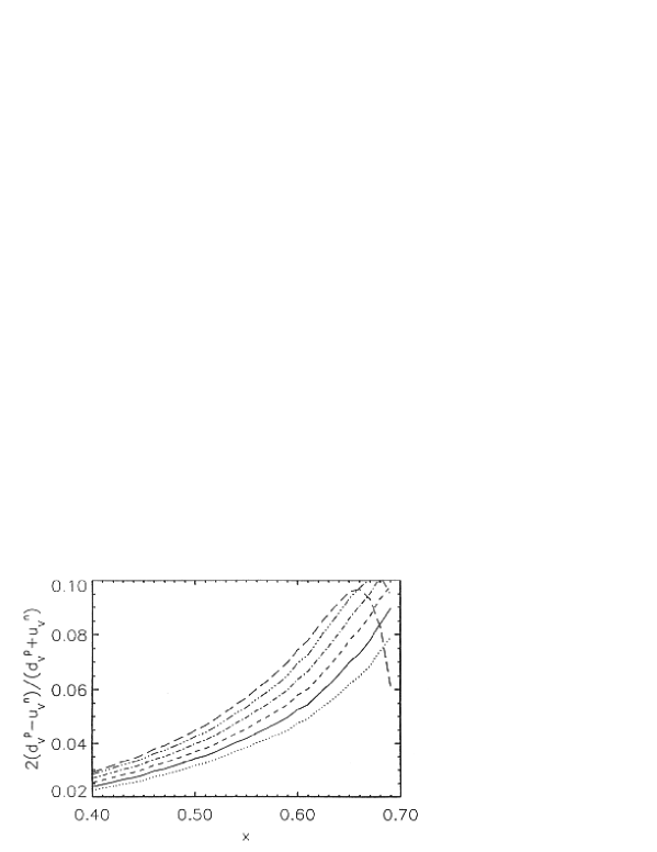
Figure 10: Model calculation of percent minority valence quark CSV term, $\delta d_{v}(x)/d_{v}(x)$ vs. $x$, evolved to $Q^{2}=10$ GeV². From Ref. [7].

Why should the minority valence quark CSV, $\delta d_{\rm v}(x)$, be a much larger percentage at large $x$ than the majority CSV term, $\delta u_{\rm v}(x)$? We can understand this qualitatively because the dominant source of CSV is the mass difference of the residual diquark pair when one quark is hit in the deep-inelastic process. For the majority quark distribution, the diquark pair is $ud$ for both proton and neutron, as can be seen from Fig. 6. Consequently there is no CSV contribution from this term. For the minority quark distribution the residual diquark is $uu$ in the proton, and $dd$ in the neutron. Thus, in the difference, $d^{p}_{\rm v}(x)-u^{n}_{\rm v}(x)$, the up-down mass difference enters twice. Including electromagnetic effects, we know that the diquark mass difference is $\delta M_{2}=M_{2}^{dd}-M_{2}^{uu}\approx 4$ MeV. From Eq. 42, we can see that the valence quark distribution $q_{\rm v}(x)$ will peak at roughly $x_{peak}\sim 1-M_{2}/M$ where $M$ is the nucleon mass. For the minority quark distribution, say, $d_{\rm v}^{p}(x)$, the lowest diquark state for the $uu$ pair will be $S=1$ by the Pauli principle. From the $N-\Delta$ mass splitting we know that an $S=1$ diquark pair will have an effective mass $M_{2}(S=1)\sim 800$ MeV, while the $S=0$ diquark (which is present only for the majority quark term $u_{\rm v}^{p}(x)$) has a mass $M_{2}(S=0)\sim 600$ MeV.

As was pointed out by Close and Thomas [43], this explains why the down quark distribution $d_{\rm v}^{p}(x)$ peaks at a value $x\sim 0.1$, while the up valence quark distribution $u_{\rm v}^{p}(x)$ peaks at $x\sim 0.3$. It also predicts that $d_{\rm v}^{p}(x)<<u_{\rm v}^{p}(x)$ at large $x$, as is observed experimentally. We can obtain an estimate of the magnitude of minority quark charge symmetry breaking,

$${\delta d_{\rm v}(x)\over d_{\rm v}^{p}(x)}\approx{\delta M_{2}\over M-M_{2}}$$ (45)

Eq. 45 gives an estimate of about 4% for minority quark CSV. This can be compared with the 3-7% estimates of CSV by Sather [18], Rodionov et al. [19], and Benesh and Goldman [37].

Fig. 10 shows the fractional minority quark CSV term, $2(d^{p}_{\rm v}-u^{n}_{\rm v})/(d^{p}_{\rm v}+u^{n}_{\rm v})$ vs. $x$ for several values of the intermediate mean diquark mass. Although the precise value of the minority quark CSV changes with mean diquark mass, the size is always roughly the same and the sign is unchanged. This shows that “smearing” the mean diquark mass will not dramatically diminish the magnitude of the minority quark CSV term (the mean diquark mass must be roughly 800 MeV in the $S=1$ state to give the correct $N-\Delta$ mass splitting).

We reiterate that the magnitude of charge symmetry violation, predicted for the “minority” valence quarks at large $x$, is both extremely large and surprising. First, since the integral over $x$ of the valence quark CSV term is zero, as given in Eq. 44, large CSV contributions to valence quark parton distributions do not necessarily imply large charge symmetry violation at low energies. Second, experimental verification of these CSV effects is not a simple matter. Since we predict that charge symmetry is well obeyed for the majority valence quarks, finding CSV effects requires experiments which are sensitive to the minority quark distributions, in a region (large Bjorken $x$) where the minority quark distributions are much smaller than the majority quark terms. In Sects. 4 and 5, we will review the current experimental limits on parton charge symmetry, and suggest experiments which would be sensitive to our predicted effects.

However, as we have tried to emphasize, our predictions of charge symmetry violation depend on rather simple assumptions, which have been shown to produce reasonable parton distributions [38, 39]. Furthermore, all theoretical calculations of parton charge symmetry obtain the same qualitative result: that the percentage of CSV for minority valence quarks should be substantially larger than the fraction of majority quark CSV at large $x$ [18, 19, 37]. To state this another way, theory predicts that $\delta d_{\rm v}(x)\approx-\delta u_{\rm v}(x)$; however, at large $x$ $d_{\rm v}(x)<<u_{\rm v}(x)$, so the fraction of minority quark CSV will be substantially larger than for majority quarks. In particular, the calculation of Sather [18] gave what was essentially a model-independent estimate of parton CSV. Sather also predicted that minority quark CSV effects should be, relatively, substantially larger than majority quark CSV. This gives us confidence that our predictions are robust.

Finally, since all phenomenological fits to date assume parton charge symmetry at the outset, existing parton distributions then have CSV effects included implicitly. As we pointed out in Sect. 2, a truly consistent treatment of these effects would begin at the outset with charge asymmetric parton distributions and proceed to fit experimental data, without making the prior assumption of charge symmetry. Then the CSV contributions could be deduced in a consistent fashion. In the absence of such a consistent procedure, our calculations of charge symmetry violation should be taken as order of magnitude estimates only. This is a difficult process, and we assume it will not take place until there is some definite experimental evidence of charge symmetry violation in parton distributions.

3.2 Estimate of Charge Symmetry Violation for Sea Quarks

In the preceding section, we made estimates of valence quark charge symmetry violation, using a formalism for quark distributions which was guaranteed to produce the proper support. We could use the same formalism to calculate antiquark distributions,

$$\overline{q}(x,\mu^{2})=M\sum_{X}\,|<X|\psi^{\dagger}_{+}(0)|N>|^{2}\,\delta(M(1+x)-p_{X}^{+})$$ (46)

We would proceed with the same assumptions as for valence quarks: we would take light cone quark momentum wave functions from simple models, and truncate the sum over states in Eq. 46 to the lowest energy states which can contribute.

Recently, such a procedure has been followed by Benesh and Londergan [44]. One is confident that reasonably model-independent estimates can be made for valence quark CSV. This is borne out by substantial agreement between various theoretical results. Calculations of sea quark CSV require some additional assumptions, and the model dependence of sea quark CSV is not entirely clear. However, in these calculations one predicts that charge symmetry violation for antiquarks should be very small, probably at least an order of magnitude smaller than the corresponding effects for valence quarks.

We can give simple qualitative arguments why sea quark CSV effects should be small. The relative magnitude of CSV effects will be given approximately by

$${\delta\bar{q}\over\bar{q}}\sim{\delta M\over M}~{}~{},$$ (47)

where $M$ is the energy of the lowest intermediate state in Eq. 46, and $\delta M$ is the mass difference for intermediate states related by charge symmetry. For antiquarks, the lowest energy states which contribute are four-quark states, whose energy is roughly twice the energy of the lowest diquark states which contribute for the valence quarks. We estimate the mass difference between charge symmetric four quark states as $\delta M\approx 1.3$ MeV, or three times smaller than the mass difference for minority valence quarks. Thus, a naive expectation would be that CSV effects for sea quarks would be at least a factor of six smaller than for minority valence quarks.

In their calculations Benesh and Londergan [44] typically obtained estimates for sea quark CSV at least an order of magnitude smaller than those for valence quark CSV effects. As a result, in subsequent sections we will occasionally neglect sea quark CSV effects relative to valence quark CSV terms. Benesh and Londergan also obtain $\delta\bar{u}(x)\approx-\delta\bar{d}(x)$; therefore, one would expect that observables proportional to the difference between up and down sea quark CSV distributions would be significantly larger than observables which measure the sum of sea quark CSV terms. In Sects. 6 and 7 we review parton sum rules. There we will show that, in principle, it would be possible to get explicit measurements of charge symmetry and/or flavor symmetry violation in parton distributions, by measuring appropriate integrals of deep inelastic cross sections.

4 Present Experimental Limits on Parton Flavor Symmetry and Charge Symmetry

In this section, we review the limits we can place on parton flavor symmetry in the proton sea, and on charge symmetry of parton distributions. In the following section, we propose a series of experiments which could in principle sharpen the limits on CSV in parton distribution, and which could also discriminate between flavor symmetry and charge symmetry violation.

4.1 Drell-Yan Tests of Flavor Symmetry in the Proton Sea

Recently, there has been much interest in the details of proton sea quark distributions. The NMC experiment [4, 45] measured the $F_{2}$ structure functions for muons on proton and deuteron targets. With these data they were able to test the Gottfried Sum Rule [3], which requires the integral of the difference between proton and neutron $F_{2}$ structure functions. The experimental value $S_{G}=0.235\pm 0.026$ is more than four standard deviations below the “naive” expectation of 1/3. Both the experimental and theoretical situations are summarized in detail in the recent review by Kumano [46]. We review the Gottfried Sum Rule in Sect. 6.1.

The most likely cause for the NMC result is a substantial difference in the $\bar{d}$ and $\bar{u}$ distributions in the proton. The NMC experiment suggests that

$$\int_{0}^{1}\,dx\,\left[\bar{d}^{p}(x)-\bar{u}^{p}(x)\right]\, {CS\atop=} \,0.147\pm 0.039$$

There is no leading order QCD correction to the Gottfried Sum Rule. Ross and Sachrajda [47] showed that higher order perturbative QCD contributions lead to a value much smaller than this. Consequently, there has been much interest in experiments which might give a “direct” measurement of the sea quark distributions $\bar{d}^{p}(x)$ and $\bar{u}^{p}(x)$, and which might map out their $x$ dependence (the NMC experiment gives only the integral over $x$ of this difference).

Ellis and Stirling [13] suggested that this could be measured by comparing Drell-Yan processes initiated by protons, on proton and deuteron targets. We review here the information which could be obtained from these measurements.

In the Drell-Yan [DY] process [48] one observes lepton pairs of opposite charge and large invariant mass which arise from hadronic collisions. This process occurs when a quark (antiquark) from the projectile annihilates an antiquark (quark) of the same flavor from the target. This produces a virtual photon which subsequently decays into a pair of charged leptons. The process is shown schematically in Fig. 11a, for $NN$ DY processes. A quark in one nucleon annihilates an antiquark of the same flavor in the other nucleon. In Fig. 11b we show the corresponding DY process for $\pi^{+}+p$ reactions, in the valence region for both particles.

The Drell-Yan process for the interaction of hadron $A$ with hadron $B$ has the form

$${d^{2}\sigma^{AB}\over dx_{1}\,dx_{2}}={4\pi\alpha_{s}^{2}\over 9sx_{1}\,x_{2}}\,K(x_{1},x_{2})\sum_{i}\,e_{i}^{2}\left[q^{A}_{i}(x_{1})\bar{q}^{B}_{i}(x_{2})+\bar{q}^{A}_{i}(x_{1})q^{B}_{i}(x_{2})\right]$$ (48)

In Eq. 48, $s$ is the square of the CM energy, and $x_{1}$ and $x_{2}$ are, respectively, the longitudinal momentum fractions carried by the target (projectile) quarks (or antiquarks) of flavor $i$ and charge $e_{i}$. For example, the quantity $\bar{q}^{B}_{i}(x_{2})$ is the antiquark distribution of the target for quarks of flavor $i$ and momentum fraction $x_{2}$. The factor $K(x_{1},x_{2})$ accounts for the higher-order QCD corrections which enter the DY process. Detailed reviews of their form can be found in several articles [20, 21].

                      

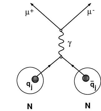
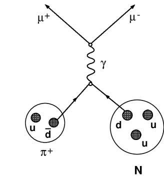
Figure 11: Schematic picture of Drell-Yan [DY] process for two hadrons. (a) $NN$ DY is sensitive to antiquarks in one nucleon; (b) $\pi^{+}-p$ DY process, in the valence region for both particles.

The values of $x_{1}$ and $x_{2}$ can be extracted from experiment through the equations

$$M^{2} = sx_{1}x_{2}\approx 2P_{\ell^{+}}P_{\ell^{-}}\left(1-\cos\theta_{\ell^{+}\ell^{-}}\right)$$

$$x_{F} \equiv x_{1}-x_{2}={2\left(P_{\ell^{+}}+P_{\ell^{-}}\right)_{L}\over s}-1$$

$$\tau = x_{1}\,x_{2}$$

$$y = {\ln\left(x_{1}/x_{2}\right)\over 2}$$ (49)

In Eq. 49, $P_{\ell^{+}}$ and $P_{\ell^{-}}$ are respectively the laboratory momenta of the outgoing leptons, $\left(P_{\ell^{+}}+P_{\ell^{-}}\right)_{L}$ is the longitudinal momentum of the lepton pair, and $\theta_{\ell^{+}\ell^{-}}$ is the angle between their momentum vectors.

The experiments have compared Drell-Yan cross sections for incident protons on proton and deuterium targets. Taking ratios of Drell-Yan cross sections avoids the necessity for precise knowledge of the factor $K$ in Eq. 48. Assuming the validity of the impulse approximation, the DY cross section on the deuteron is just the sum of the DY cross sections on the free proton and neutron. In that case the DY cross sections are proportional to

$$\sigma_{DY}^{pp} \sim {4\over 9}\left[u^{p}(x_{1})\bar{u}^{p}(x_{2})+\bar{u}^{p}(x_{1})u^{p}(x_{2})\right]+{1\over 9}\left[d^{p}(x_{1})\bar{d}^{p}(x_{2})+\bar{d}^{p}(x_{1})d^{p}(x_{2})\right]$$

$$\sigma_{DY}^{pD} \sim {4\over 9}\left[u^{p}(x_{1})\left(\bar{u}^{p}(x_{2})+\bar{u}^{n}(x_{2})\right)+\bar{u}^{p}(x_{1})\left(u^{p}(x_{2})+u^{n}(x_{2})\right)\right]$$ (50)

$$+ {1\over 9}\left[d^{p}(x_{1})\left(\bar{d}^{p}(x_{2})+\bar{d}^{n}(x_{2})\right)\bar{d}^{p}(x_{1})\left(d^{p}(x_{2})+d^{n}(x_{2})\right)\right]$$

If we assume charge symmetry then Eq. 50 reduces to

$$\sigma_{DY}^{pD}\, {CS\atop\sim} \,\left({4\over 9}u^{p}(x_{1})+{1\over 9}d^{p}(x_{1})\right)\left(\bar{u}^{p}(x_{2})+\bar{d}^{p}(x_{2})\right)$$ (51)

$$+ \left({4\over 9}\bar{u}^{p}(x_{1})+{1\over 9}\bar{d}^{p}(x_{1})\right)\left(u^{p}(x_{2})+d^{p}(x_{2})\right)$$

The physics is most clear if we go to large $x_{1}$, i.e. large $x$ for the projectile proton, and substantially smaller $x_{2}$ for the target. In this regime the probability for finding antiquarks in the projectile is extremely small, so as a good approximation the DY process proceeds by quarks in the projectile annihilating antiquarks in the target. In this region the ratio of DY processes on the deuteron, to those from the proton, are given by

$$R_{sea}(x_{1},x_{2})={\sigma^{pD}_{DY}(x_{1},x_{2})\over 2\sigma^{pp}_{DY}(x_{1},x_{2})}\, {CS\atop=} \,{1\over 2}{\left(1+\bar{R}(x_{2})\right)\left(1+r(x_{1})/4\right)\over\left(1+r(x_{1})\bar{R}(x_{2})/4\right)}\quad,$$ (52)

In Eq. 52, we define the ratios

$$\bar{R}(x) = {\bar{d}^{p}(x)\over\bar{u}^{p}(x)}$$

$$r(x) = {d^{p}(x)\over u^{p}(x)}$$ (53)

From Eqs. 52 and 53 we see that if $\bar{d}^{p}(x)=\bar{u}^{p}(x)$ for some $x=x_{e}$, then $R_{sea}(x_{1},x_{e})=1$. For large $x$, the ratio $r(x)$ is small (the probability of finding an up quark in the proton at large $x$ is significantly higher than for finding a down quark). In that case, as $x_{1}\rightarrow 1$, we have

$$R_{sea}(x_{1},x_{2})\, {CS\atop\longrightarrow} \,{1\over 2}\left(1+\bar{R}(x_{2})\right)\left(1+{r(x_{1})\over 4}\left[1-\bar{R}(x_{2})\right]\right)\quad,$$ (54)

From Eq. 54, we see that the ratio of DY cross sections in this kinematic region should directly measure the ratio of the down antiquark to up antiquark distributions in the proton, at a given value of $x_{2}$. Neglecting terms of order $r(x_{1})$, the quantity $R_{sea}(x_{1},x_{2})$ would be less than one if $\bar{d}^{p}(x_{2})<\bar{u}^{p}(x_{2})$, and greater than one if $\bar{d}^{p}(x_{2})>\bar{u}^{p}(x_{2})$. There have been three recent experiments which enable us to extract the difference between down and up antiquark distributions in the proton.

The experiment E772 at FNAL [49] measured Drell-Yan processes for 800 GeV protons on a variety of nuclear targets. The targets employed were D, C, Ca, Fe, and W. As there was no proton target, the $D/p$ ratio could be inferred by comparing the isoscalar targets with those for which $N\neq Z$. For non-isoscalar targets the excess neutron fraction is proportional to $\epsilon=(N-Z)/A$. As $\epsilon$ is rather small for these targets, it is difficult to measure neutron/proton differences, and hence hard to isolate any difference between down and up antiquarks in the proton. The experimental results appeared to show differences between $\bar{d}^{p}$ and $\bar{u}^{p}$ [49], and did disagree with some theoretical suggestions for $\bar{d}^{p}/\bar{u}^{p}$, but it was hard to draw any firm conclusions regarding this question from the E772 experiment.

Experiment NA51 at CERN [14] measured Drell-Yan processes for 450 GeV protons on proton and deuteron targets. The NA51 data looked primarily at symmetric kinematics $x_{1}=x_{2}$. The symmetric geometry is particularly good for minimizing errors in comparison of different experiments. For this geometry the approximations used to generate Eq. 52 are not valid. Instead, Ellis and Stirling [13] showed that for symmetric kinematics the ratio of Drell-Yan cross sections could be written as

$$R_{sea}(x_{1}=x_{2}=x)\, {CS\atop=} \,{\sigma^{pD}_{DY}(x,x)\over 2\sigma^{pp}_{DY}(x,x)}={1\over 2}\left(1+{{5\over 8}\left(\bar{R}(x)+r(x)\right)\over\left(1+r(x)\bar{R}(x)/4\right)}\right)\quad,$$ (55)

The NA51 group obtained a ratio for a single averaged point $<x>=0.18$. From their measured asymmetry in Drell-Yan processes, they extracted the value

$${\bar{u}^{p}\over\bar{d}^{p}}|_{<x>=0.18}=0.51\pm 0.04(stat)\pm 0.05(syst)$$ (56)

The NA51 result, although for only a single average $x$ value, suggests that there are twice as many down antiquarks as up antiquarks at $x=0.18$.

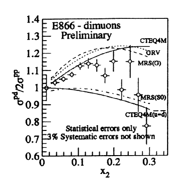
Figure 12: The ratio of pD to pp DY cross sections as a function of target $x_{2}$, preliminary results of the E866 Collaboration, Ref. [15]. Curves are for phenomenological parton distributions.

The E866 group at FNAL [15] compared Drell-Yan processes for 800 GeV protons on liquid hydrogen and Deuterium targets. The E866 experiment has both the high statistics and the wide kinematic range which made it difficult for prior experiments to investigate this issue. In Fig. 12 we show preliminary results from E866 for the ratio of DY cross sections $\sigma^{pD}/2\sigma^{pp}$, for positive $x_{F}=x_{1}-x_{2}$. In this kinematic region we expect the antiquarks to come predominantly from the target. For lower values of $x_{2}$ the ratio is greater than one, and (with large errors) appears to decrease at higher values of $x_{2}$. Where the ratio exceeds one, from Eq. 54 this implies $\bar{d}^{p}(x)>\bar{u}^{p}(x)$. Furthermore, with this data one can map out the difference between $\bar{d}^{p}(x)$ and $\bar{u}^{p}(x)$ over a substantial region of $x$.

The curves in Fig. 12 are from phenomenological parton distributions [50, 51, 52]. The upper curves allow $\bar{d}^{p}(x)\neq\bar{u}^{p}(x)$, while the lower curves constrain the up and down sea quark distributions to be identical. For $x_{2}<0.2$, the ratio of DY cross sections is clearly greater than one. In the following subsection we discuss the implications of the E866 results, and we examine several theoretical models which might generate large flavor symmetry violation in the nucleon sea.

4.2 Implications of Large Flavor Symmetry Violation from Drell-Yan Experiments

The experimental Drell-Yan results appear to show a substantial violation of flavor symmetry in the proton sea. The preliminary results of FNAL experiment E866 [15] are most definitive in this regard, as they can extract $\bar{d}^{p}(x)/\bar{u}^{p}(x)$ over a substantial range of $x$. In Fig. 13 we plot the ratio $\bar{d}^{p}(x)/\bar{u}^{p}(x)$ vs. $x$ which has been extracted from the (preliminary) E866 data [15].

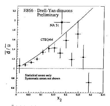
Figure 13: The ratio $\bar{d}^{p}(x)/\bar{u}^{p}(x)$ extracted from preliminary E866 results of Fig. 12.

The FSV contribution seen in the Drell-Yan experiments is surprisingly large, as it is much larger than can be accommodated by perturbative QCD. Both NLO and NNLO QCD calculations have been carried out, and predict very small FSV effects. Ross and Sachrajda [47] showed that the flavor symmetry violating contribution which arises from higher order QCD evolution is very small (for a comprehensive review of theoretical estimates of FSV, see the review by Kumano [46]). Consequently, we need a non-perturbative mechanism to generate flavor-violating sea quark distributions which will reproduce the experimental result.

Several authors (see the review by Kumano [46] for references) have investigated mechanisms for producing a large excess of $\bar{d}$ over $\bar{u}$ in the proton. Since there are two valence up quarks and one valence down quark in the proton, the Pauli principle should make it easier to form a $d\bar{d}$ pair than a $u\bar{u}$ pair in the presence of the valence quarks (one should be somewhat careful of statements like this: a recent paper by Steffens and Thomas [53] suggests that $u\bar{u}$ pairs may in fact be favored if all antisymmetrization terms are considered). In Feynman and Field’s early paper on parton distributions [54], they assumed an excess of $\bar{d}$ quarks in the proton on these grounds.

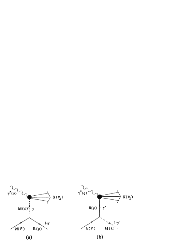
Figure 14: Schematic picture of “mesonic” contributions to DIS for a nucleon. a) virtual meson contribution; b) recoil baryon contribution.

Another mechanism for generating additional $\bar{d}$ quarks in the proton is due to the “Sullivan Effect” [55], whereby the virtual photon can couple to a meson created by a quark. Thomas [56] pointed out in 1983 that “pionic” effects would produce an excess of $\bar{d}$ over $\bar{u}$ in the proton. The basic mechanism is shown in Fig. 14. A proton fragments into a neutron and a $\pi^{+}$. If the virtual photon scatters from the down antiquark in the $\pi^{+}$, it will produce an excess of $\bar{d}$ over $\bar{u}$.

Several authors have shown that effects given by the “Sullivan” process can produce an excess of $\bar{d}$ quarks in the proton sea. Detailed reviews of this process, and of the literature on this subject, are given by Kumano [46], and by Speth and Thomas [57]. The original papers [56] considered the contributions to this process from excess pions in the nucleus. Kumano and Londergan [11] calculated a model which included contributions from pions, nucleons and $\Delta$ isobars (the $\Delta$ contribution tends to cancel the nucleon-only contribution at larger $x$). This relatively simple model has been expanded by the Adelaide [40] and Jülich [58] groups to include all of the meson and baryon states normally associated with “meson-exchange” models.

The “mesonic” models look promising, in that both the magnitude of this effect, and the $x$-dependence of the predicted $\bar{d}^{p}/\bar{u}^{p}$ difference, are in qualitative agreement with experiment. In Fig. 13, the solid curve is the CTEQ4M phenomenological parton distribution [50]. This is quite similar to the ‘mesonic’ model result of the Jülich group [58] for the ratio of down to up antiquark distributions. The model of Kumano and Londergan [11], which has only $\pi$ and $\Delta$ in addition to the nucleon, is similar to the CTEQ4M prediction at small $x$ but gives a smaller ratio at large $x$. Both mesonic calculations correctly predict the excess $\bar{d}^{p}(x)>\bar{u}^{p}(x)$, and both get the general shape of the down antiquark excess as a function of $x$. At larger $x$ the error bars are sufficiently large that detailed comparisons are difficult. Furthermore, the mesonic models are very sensitive to small changes in the $\pi N\Delta$ coupling constant, and to the shapes of the $NN\pi$ and $N\Delta\pi$ form factors.

There are also other theoretical models which predict an excess of $\bar{d}$ antiquarks in the proton. Eichten, Hinchliffe and Quigg [59] have investigated the contribution from a model in which quarks couple chirally to pions . Dong and Liu [60] estimate the contributions from mesons in lattice gauge calculations. They try to separate the contributions from “cloud” antiquarks and “sea” antiquarks in a lattice calculation. It is not possible to make a precise separation on the lattice, but their calculations also suggest an excess of down antiquarks relative to up antiquarks. All of this work is summarized in Kumano’s review article [46]. One additional possibility is that instanton condensates in the nucleon [61, 62] might produce an excess of down sea quarks relative to up sea quarks in the proton.

The Drell-Yan experiments appear to show conclusively a large violation of flavor symmetry in the proton sea. However, it is important to note that all these results depend on the assumption of parton charge symmetry. If one relaxes this assumption, one could in principle reproduce the Drell-Yan results even if flavor symmetry is exact. From Eq. 50, let us assume exact flavor symmetry in the proton sea, i.e.

$$\bar{u}^{p}(x) = \bar{d}^{p}(x)\equiv\bar{q}^{p}(x)$$

$$\bar{u}^{n}(x) = \bar{d}^{n}(x)\equiv\bar{q}^{n}(x)$$

$$\bar{q}^{p}(x) \neq \bar{q}^{n}(x)$$ (57)

The parton distributions of Eq. 57 are completely flavor symmetric but not charge symmetric. If we go to the region $x_{F}>0$ we find that Eq. 54 now becomes

$$R_{sea}(x_{1},x_{2})\, {FS\atop\rightarrow} \,{1\over 2}\left(1+{\bar{q}^{n}(x_{2})\over\bar{q}^{p}(x_{2})}\right)\quad.$$ (58)

The Drell-Yan experiments could thus be reproduced, even if flavor symmetry was exact, with a sufficiently large violation of charge symmetry in the parton distributions. It would require an astonishingly large CSV contribution in the nucleon sea to reproduce the E866 results: this would be a factor 25-50 larger than our estimates in Sect. 3. Alternatively, the E866 results could be due to a linear combination of FSV and CSV effects in the nucleon sea.

In the next subsections, we will review the experimental constraints on charge symmetry in parton distributions. In Sect. 5, we will suggest a number of new experiments which might provide more stringent tests of parton charge symmetry.

4.3 The “Charge Ratio:” Comparison of Muon with Neutrino Induced Structure Functions

In Sect. 2.5, we derived the relation between the structure function $F_{2}$ measured in neutrino induced charged current reactions, and the $F_{2}$ structure function for charged lepton DIS, both measured on isoscalar targets. From Eq. 36, at sufficiently high energies the structure functions have the form

$$F_{2}^{\gamma N_{0}}(x) = x\left[{5\over 18}\,\overline{Q}(x)-{1\over 6}\left(s(x)+\bar{s}(x)\right)-{4\delta d(x)+4\delta\bar{d}(x)+\delta u(x)+\delta\bar{u}(x)\over 18}\right]$$

$$\overline{F_{2}}^{WN_{0}}(x) = x\left[\overline{Q}(x)-{\delta d(x)+\delta\bar{d}(x)+\delta u(x)+\delta\bar{u}(x)\over 2}\right]$$

$$\overline{Q}(x) = \sum_{j=u,d,s,c}q_{j}(x)+\overline{q}_{j}(x)$$

$$\widetilde{Q}(x) \equiv \overline{Q}(x)-{3\left(s(x)+\bar{s}(x)\right)\over 5}$$ (59)

In Eq. 59 we have neglected the charmed quark contribution to the structure functions, and for the moment we have set $R=0$. The function $\overline{F_{2}}^{WN_{0}}(x)$ is the average of the neutrino and antineutrino induced charged current structure functions.

From Eq. 59 we see that there is a simple relation between the two structure functions, in the limit of exact charge symmetry. The ratio of the two structure functions in Eq. 59, when corrected for the strange quark contribution and the factor $5/18$ (which reflects the fact that the virtual photon couples to the squared charge of the quarks while the weak interactions couple to the weak isospin), is defined as the “charge ratio” $R_{c}(x,Q^{2})$ or, as it is sometimes termed, the “5/18^th rule.” This quantity should be one, independent of $x$ and $Q^{2}$, in the naive parton model. If we expand the ratio $R_{c}$ to lowest order in the presumably small charge symmetry violating terms, we obtain

$$R_{c}(x) \equiv {F_{2}^{\gamma N_{0}}(x)\over{5\over 18}\overline{F_{2}}^{WN_{0}}(x)-x\left(s(x)+\bar{s}(x)\right)/6}$$ (60)

$$\approx 1+{3\left(\delta u(x)+\delta\bar{u}(x)-\delta d(x)-\delta\bar{d}(x)\right)\over 10\widetilde{Q}(x)}$$

As we pointed out in Section 2.6, the strange quark distributions can be obtained independently by measuring opposite sign dimuon events in neutrino DIS from nuclei. Using these strange quark distributions in Eq. 60, and comparing the $F_{2}$ structure functions for lepton-induced processes with the $F_{2}$ structure functions from weak processes mediated by $W$-exchange, we can in principle measure parton charge symmetry violation and determine its $x$ dependence. By measuring $R_{c}(x)$ we can place upper limits on parton CSV as a function of $x$. The longitudinal/transverse ratio $R$ can be included in forming the structure functions, and will cancel when the ratio $R_{c}$ is taken.

Eq. 60 requires averaging the $F_{2}$ structure functions for neutrino and antineutrino cross sections. If we instead take the ratio using only neutrino-induced reactions, it is straightforward to obtain

$$R_{c}^{\nu}(x) \equiv {F_{2}^{\gamma N_{0}}(x)\over{5\over 18}F_{2}^{W^{+}N_{0}}(x)-x\left(s(x)+\bar{s}(x)\right)/6}$$ (61)

$$\approx 1-{s(x)-\bar{s}(x)\over\widetilde{Q}(x)}+{\left(4\delta u(x)-\delta\bar{u}(x)-4\delta d(x)+\delta\bar{d}(x)\right)\over 5\widetilde{Q}(x)}$$

Eq. 61 differs from Eq. 60 since it has a term proportional to the difference between strange and antistrange quark distributions, and also in the relative weighting of the CSV terms which enter. The $s-\bar{s}$ term is absent if one is able to average neutrino and antineutrino cross sections.

The charge ratio test allows us to place the strongest limits to date on parton CSV. There should be no additional QCD corrections to this relation so it should be independent of $Q^{2}$, provided that the structure functions are calculated in the so-called “DIS scheme.” In this scheme, the $F_{2}$ structure functions are defined so that they have the form $F_{2}(x)=x\sum_{i}e_{i}^{2}[q_{i}(x)+\bar{q}_{i}(x)]$ to all orders, where $e_{i}$ is the quark charge appropriate for either the electromagnetic or weak interactions. For example, the CTEQ4D parton distributions [50] were determined in the DIS scheme. Despite the robustness of the charge ratio test, it also depends on a large number of assumptions and corrections, which must be taken into account to obtain limits on CSV terms. Among these corrections are:

• Relative normalization between leptonic and neutrino cross sections.

• Corrections due to strange quarks. As outlined in Sect. 2.6, $s(x)$ ($\bar{s}(x)$) can be independently extracted from the cross section for opposite sign dimuons from reactions induced by neutrinos (antineutrinos)

• Corrections from excess neutrons. Eq. 60 was derived for isoscalar targets. In order to obtain reasonable cross sections, neutrino reactions are now measured on iron targets. This requires a correction for the excess neutrons in the target.

• Heavy target corrections. If the leptonic structure functions are obtained from light targets and neutrino reactions performed on heavy targets, it is necessary to correct the neutrino $F_{2}$ structure functions for heavy target effects. At low and intermediate $x$, heavy target structure functions are decreased because of shadowing and EMC effects, respectively; at very large $x$ Fermi motion effects increases the structure functions for heavy targets.

• Higher twist effects on parton distributions.

• Heavy quark threshold effects. At sufficiently low energies, heavy quark threshold effects will modify structure functions, as we reviewed in Sect. 2.2.

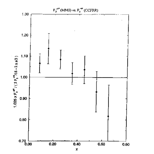
Figure 15: Charge ratio $R_{c}^{\nu}(x)$ of Eq. 61 vs. $x$. Muon measurements of Meyers et al, Ref. [63] [using muons on Fe at FNAL], with CCFRR neutrino measurements on iron, Ref. [64].

In Fig. 15 we plot the charge ratio $R_{c}^{\nu}$, i.e. the ratio of muon $F_{2}$ structure functions measured by Meyers et al. on iron [63] to the value of $F_{2}$ extracted from the CCFRR neutrino measurements [64]. The muon measurements were taken at FNAL with 93 and 215 GeV muons, using the multimuon spectrometer at FNAL. The CCFRR neutrino measurements were made with the FNAL narrow-band neutrino beam.

In comparing the muon and neutrino measurements, the following corrections were made by Meyers et al.. First, the $F_{2}$ structure functions were modified by including the strange quark contribution, determined as described in Section 2.6 [30]. Second, corrections were made for the excess neutrons in iron. Third, there was a discrepancy in the extraction of the $F_{2}$ structure functions. The muon data were analyzed assuming longitudinal/transverse ratio $R=0$, while the neutrino data assumed $R=0.1$. Meyers et al. corrected the muon data to make them consistent. The muon data have been renormalized by the factor 1.025.

Within the errors (two standard deviations), $R_{c}^{\nu}$ is consistent with unity, except possibly at the largest value of $x$ where $R_{c}^{\nu}(x=0.65)=0.82\pm 0.09$. From these experiments, the upper limits on the CSV contribution to $R_{c}$ are generally no better than about 10%, and at large values of $x$ the errors are significantly larger. The experimental data is consistent with zero charge symmetry violation and certainly rules out any extremely large violation of parton charge symmetry. From Eq. 61 and the theoretical calculations of parton CSV given in Sect. 3, we expect that the CSV contribution to the charge ratio will not exceed 1-2% at any value of $x$. Consequently, any deviation of the charge ratio from unity, at any value of $x$, would be surprising and very interesting.

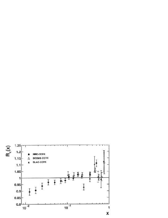
Figure 16: Charge ratio $R_{c}^{\nu}(x)$ of Eq. 61 vs. $x$. CCFR neutrino measurements on iron with the FNAL wide-band neutrino beam, Ref. [95]. Circles: $\mu+D$ measurements of the NMC group, Ref. [4]; open triangles, muon measurements from the BCDMS group on deuterium, Ref. [66] and carbon, Ref. [67]; solid triangles: SLAC electron scattering data, Ref. [24, 68].

More recent data for both muons and neutrinos allows us to make substantially more precise tests of parton charge symmetry. The NMC group [4] measured the $F_{2}$ structure function for muon interactions on deuterium at energy $E_{\mu}=90$ and 280 GeV. The CCFR group [65] has extracted the $F_{2}$ structure function for neutrino and antineutrino interactions on iron using the Quadrupole Triplet Beam at FNAL. The CCFR measurements provide the most copious sample of neutrino events, and allow the most precise limits on parton CSV. In Fig. 16 we plot the charge ratio $R_{c}$ of Eq. 60 vs. $x$. The circles are the NMC/CCFR ratio. The open triangles are the BCDMS/CCFR charge ratio, where BCDMS represents the muon scattering results of the BCDMS group on deuterium [66] and carbon [67]. The solid triangles are the SLAC/CCFR charge ratio, where SLAC denotes electron scattering results of the SLAC group [24, 68].

The charge ratio has been calculated by C. Boros [69]. The results differ somewhat from those produced by Seligman et al. in their calculation of the charge ratio [65, 70]. In comparing the data sets, Boros takes only those points with the same $x$ value and sums over overlapping $Q^{2}$ values, while Seligman interpolates between measured values of the structure functions. In addition, in Fig. 16 there is no correction for strange quarks.

In the region $0.1\leq x\leq 0.4$, the charge ratio test is consistent with unity, and the data gives an upper limit to CSV effects in the charge ratio at about the 3% level. For larger values of $x$ the upper limit on CSV effects is more consistent with the 5-10% level, due mainly to the poorer statistics and, as we will see, on the large Fermi motion corrections needed for the heavy target at large $x$. Both the new muon and neutrino data are more precise than the older measurements. In addition, the more recent phenomenological parton distributions are better determined. Relative normalizations of lepton and neutrino cross sections appear to be well understood. All data is analyzed with consistent assumptions about the longitudinal/transverse ratio $R$. Heavy quark threshold effects should also be under control.

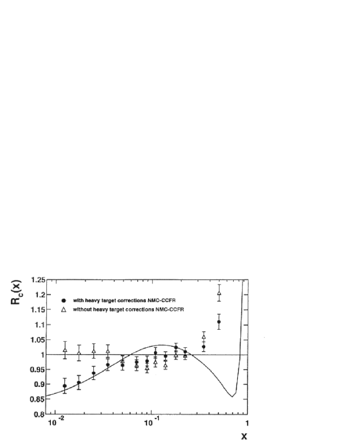
Figure 17: Effects of heavy target correction on charge ratio of Fig. 16. Triangles: NMC-CCFR data without heavy target correction; circles: NMC-CCFR data including heavy target correction (solid curve).

Probably the most significant correction is the heavy target correction, necessary because we are comparing muon data on deuterium, where the correction is presumably very small, to neutrino data on iron. In Fig. 17 we show the same charge ratio as in Fig. 16 for the NMC-CCFR comparison, but here we explicitly show the heavy target corrections. The open triangles show the ratio without heavy target corrections, and the solid circles show the ratio after applying these corrections. The solid line is the iron target correction factor as a function of $x$.

After including the heavy target correction, there appears to be a significant deviation of the charge ratio from one at the smallest values $x<0.1$; the discrepancy approaches 15% at the smallest values of $x$, with the electromagnetic structure functions being smaller than the neutrino ones. Several suggestions have been made to explain this discrepancy. We summarize the explanations listed by Seligman [65]. First, the lack of agreement could result from difficulties in analyzing the low-$x$ neutrino events. This will be tested with the next generation FNAL neutrino experiment E815. Second, it is conceivable that the disagreement arises from effects at small $Q^{2}$ which differ between leptonic and neutrino induced reactions [71]. However, these effects appear to be quite small for $Q^{2}>1$ GeV² [72].

The discrepancy increases monotonically at small $x$, where the strange quark effects are largest. One intriguing possibility is that strange quark effects might account for all of the apparent discrepancy. In this case it is possible that the present phenomenological analysis of both strange quark and antiquark distributions need to be modified substantially, as has recently been argued by Brodsky and Ma [35]. In any case, the recent NMC-CCFR comparison allows us to put rather tight upper limits on parton CSV contributions, and focuses our attention on the low-$x$ region where there is currently a discrepancy between the $F_{2}$ structure functions extracted from the two reactions.

4.4 Comparison of Neutrino and Antineutrino Cross Sections on Isoscalar Targets

On an isoscalar target, the differential cross sections for charged current reactions induced by neutrinos or antineutrinos can be written in the general form

$${d\sigma^{\nu N_{0}}\over dx} = {G^{2}M_{N}E\over\pi}\left[\left({1\over 2}+{1\over 6(1+R)}\right)F_{2}^{W^{+}N_{0}}(x,Q^{2})+{1\over 3}xF_{3}^{W^{+}N_{0}}(x,Q^{2})\right]$$

$${d\sigma^{\bar{\nu}N_{0}}\over dx} = {G^{2}M_{N}E\over\pi}\left[\left({1\over 2}+{1\over 6(1+R)}\right)F_{2}^{W^{-}N_{0}}(x,Q^{2})-{1\over 3}xF_{3}^{W^{-}N_{0}}(x,Q^{2})\right].$$ (62)

In Eq. 62, the quantity $R$ is the longitudinal/transverse ratio,

$$R(x,Q^{2})={\sigma_{L}\over\sigma_{T}}={F_{2}(x,Q^{2})-2x\,F_{1}(x,Q^{2})\over 2x\,F_{1}(x,Q^{2})}.$$ (63)

From Eq. 29 we see that the structure functions $F_{2}$ and $F_{3}$ per nucleon for an isoscalar target can be written as

$$F_{2}^{W^{+}N_{0}}(x) = x\left[u^{p}(x)+d^{p}(x)+\bar{u}^{p}(x)+\bar{d}^{p}(x)+2s(x)-\delta u(x)-\delta\bar{d}(x)\right]$$

$$F_{2}^{W^{-}N_{0}}(x) = x\left[u^{p}(x)+d^{p}(x)+\bar{u}^{p}(x)+\bar{d}^{p}(x)+2\bar{s}(x)-\delta d(x)-\delta\bar{u}(x)\right]$$

$$xF_{3}^{W^{+}N_{0}}(x) = x\left[u^{p}(x)+d^{p}(x)-\bar{u}^{p}(x)-\bar{d}^{p}(x)+2s(x)-\delta u(x)+\delta\bar{d}(x)\right]$$

$$xF_{3}^{W^{-}N_{0}}(x) = x\left[u^{p}(x)+d^{p}(x)-\bar{u}^{p}(x)-\bar{d}^{p}(x)-2\bar{s}(x)-\delta d(x)+\delta\bar{u}(x)\right].$$ (64)

In Eq. 64, we assume that the momentum transfers are sufficiently high that threshold effects can be neglected. In this equation, we have neglected the contribution from charmed quarks in the nucleon, and for the moment we have set $R=0$. In this limit, the $F_{2}$ structure functions from neutrinos and antineutrinos are identical except for CSV contributions. In addition, the $F_{2}$ and $F_{3}$ structure functions are identical except that the antiquark contributions have different signs. Consequently, if we go to large $x$ where the sea quark contributions become small with respect to the valence quark terms, then both $F_{2}$ and $F_{3}$ structure functions for both neutrinos and antineutrinos should become equal. From Eq. 62 we see that $F_{2}$ and $F_{3}$ will add together in the neutrino cross section, but will cancel in the antineutrino cross section.

We thus define the ratio of antineutrino to neutrino charged current cross sections on an isoscalar target,

$$r^{\nu/\bar{\nu}}(x)\equiv{d\sigma^{\bar{\nu}N_{0}}(x)/dx\over d\sigma^{\nu N_{0}}(x)/dx}$$ (65)

We will focus on this relation at reasonably large values of $x\geq 0.3$. For these values of $x$ the sea quark distribution will be small relative to the valence quark distributions. In this region we can expand the ratio of Eq. 65 to lowest order in small quantities, and we obtain

$$r^{\nu/\bar{\nu}}(x) \approx {1\over 3}+{8\left(\bar{u}^{p}(x)+\bar{d}^{p}(x)\right)\over 9\left(u^{p}_{v}(x)+d^{p}_{v}(x)\right)}+{\delta u(x)-\delta d(x)\over 3\left(u^{p}_{v}(x)+d^{p}_{v}(x)\right)}+{4s(x)\over 3\left(u^{p}_{v}(x)+d^{p}_{v}(x)\right)}\quad[R=0]$$

$$r^{\nu/\bar{\nu}}(x) \approx {21\over 65}+{3784\left(\bar{u}^{p}(x)+\bar{d}^{p}(x)\right)\over(65)^{2}\left(u^{p}_{v}(x)+d^{p}_{v}(x)\right)}+{21\left(\delta u(x)-\delta d(x)\right)\over 65\left(u^{p}_{v}(x)+d^{p}_{v}(x)\right)}$$ (66)

$$+ {88s(x)\over 65\left(u^{p}_{v}(x)+d^{p}_{v}(x)\right)}\quad[R=0.1]$$

In Eq. 66, we treat $R$ as a constant (we use the value averaged over $x$). If $R=0$, the ratio $r^{\nu/\bar{\nu}}(x)$ is predicted to approach the value 1/3 at large values of $x$; for $R=0.1$, the ratio should approach 21/65. $x$-dependent deviations from this constant value will arise from either sea quark or CSV contributions.

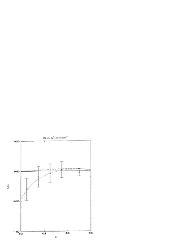
Figure 18: The quantity $1-3r^{\nu/\bar{\nu}}$ of Eq. 65, vs. $x$ for neutrino and antineutrino data on BEBC D bubble chamber. Data from WA25 experiment, Ref. [73].

At present, this ratio can be obtained from experimental data on deuterium and iron targets. In Fig. 18 we plot $1-3r^{\nu/\bar{\nu}}$ vs. $x$ for the WA25 data [73]. This consists of neutrino and antineutrino cross sections taken in the BEBC D bubble chamber at CERN. The experimental points plotted have an average momentum transfer $Q^{2}=11$ GeV². They were analyzed assuming $R=0$. The dotted curve in Fig. 18 is the total contribution from both sea quarks and our model predictions from valence quark CSV (see Section 3), while the dashed curve is the model contribution from CSV alone. The model prediction is small in absolute value, and small relative to the sea quark contribution, except at large values $x\geq 0.6$, where the CSV contribution is predicted to dominate. In the quantity $1-3r$, the sea quarks are weighted with a factor 8/3 relative to the CSV contribution. In this ratio, we predict that the sea quarks will give a negative contribution to the quantity $1-3r$, while the CSV contribution is predicted to be positive.

The experimental error bars range from about 20% at small $x$ to 50% at large $x$. The errors are substantially larger than the theoretical CSV contribution, for all measured values of $x$. If it were possible to obtain precise neutrino and antineutrino data on isoscalar targets such as D, for large values of $x$, the quantity $r^{\nu/\bar{\nu}}(x)$ could in principle give a sensitive upper limit on parton charge symmetry violation. Unfortunately, measurement of these cross sections is notoriously difficult. We know of no current plans for precision measurements of charged current cross sections for neutrino and antineutrino beams on isoscalar targets. From Fig. 18, we see that the experimental error bars would have to be at least an order of magnitude smaller than their current values to reach our predicted CSV signal. Further, it is doubtful that the neutrino results could attain the limits on CSV already reached by the “charge ratio” comparison between $F_{2}$ measurements from muons and neutrinos; this was reviewed in Sect. 4.3.

This is unfortunate, since the neutrino comparisons have fewer implicit assumptions than the charge ratio – if accurate structure functions were available for neutrino and antineutrino bombardment of isoscalar targets, one would be comparing data taken in the same experiments, one would not have to make corrections for excess neutrons, nor would one have to correct for the strange quark distributions, extracted as described in Sect. 2.6.

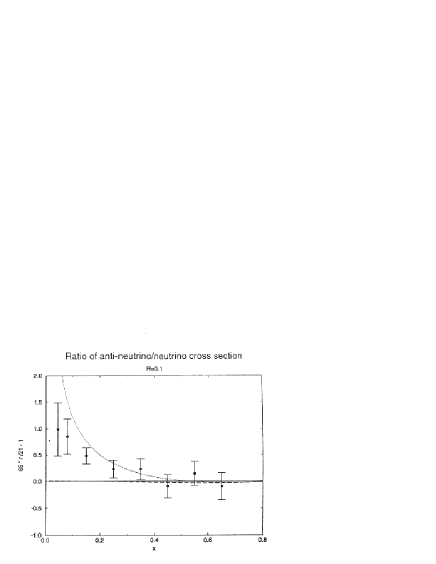
Figure 19: The quantity $1-65r^{\nu/\bar{\nu}}/21$, vs. $x$ for CCFRR neutrino and antineutrino data on iron, Ref. [64].

In Fig. 19 we plot $1-65r^{\nu/\bar{\nu}}/21$ vs. $x$ for the CCFRR data, neutrino and antineutrino cross sections on iron, taken at FNAL [64]. The plotted points correpond to an average momentum transfer $Q^{2}=12.69$ GeV². They were analyzed assuming $R=0.1$. The dotted curve in Fig. 19 is the total contribution from both sea quarks and our model predictions from valence quark CSV, while the dashed curve is the model contribution from CSV alone. The CCFRR data is similar to the WA25 results shown in Fig. 18, in that the experimental error bars are much larger than the theoretical CSV contribution, and the data is consistent with no charge symmetry violation.

The experimental error bars range from about 20% at small $x$ to 100% at large $x$. The errors are again substantially larger than the theoretical CSV contribution, for all measured values of $x$. Since iron is not an isoscalar target, it is necessary to make corrections from the excess neutrons in iron. These corrections have been taken into account in Figs. 18 and 19. There is more recent experimental data for neutrino and antineutrino cross sections from the CCFR collaboration [65]. We are unaware of a systematic study of the quantity $r^{\nu/\bar{\nu}}(x)$ by this group.

5 Proposed New Experimental Tests of Parton Charge Symmetry

In the preceding Section, we reviewed existing experiments and showed the limits they placed on charge symmetry and flavor symmetry violation in parton distributions. The latest Drell-Yan data for protons on proton and deuteron targets appear to show clear evidence of substantial flavor symmetry violation in the proton sea. However, it is conceivable (although unlikely) that this result could also be due to charge symmetry violation in parton distributions, or by some combination of flavor symmetry and charge symmetry violation. In this Section we propose a series of experiments, all of which are chosen specifically to set limits on CSV contributions to parton distributions.

5.1 Test of Weak Current Relation $F_{1}^{W^{+}N_{0}}(x)=F_{1}^{W^{-}N_{0}}(x)$

In Sect. 2.5, we reviewed the high-energy limiting form to the electroweak structure functions. We showed that, at sufficiently high energies, the charge-changing structure functions on an isoscalar target are equal except for contributions from valence quark CSV, and possible strange or charmed quark terms, i.e.

$$F_{1}^{W^{+}N_{0}}(x,Q^{2})-F_{1}^{W^{-}N_{0}}(x,Q^{2})={\delta d_{\rm v}(x)-\delta u_{\rm v}(x)\over 2}+s(x)-\bar{s}(x)-c(x)+\bar{c}(x),$$ (67)

as shown in Eq. 29.

At the enormous values of $Q^{2}$ that can be probed at HERA, weak interaction processes such as $e^{-}p\rightarrow\nu_{e}X$ are not completely negligible with respect to the electromagnetic process $e^{-}p\rightarrow e^{-}X$. Furthermore, we are well above heavy quark production thresholds, so threshold effects on the CKM matrix elements and issues like “slow rescaling” which are critical at lower energies, are unimportant in this regime. The $(e^{-},\nu_{e})$ reaction picks out the positively charged partons in the target, so that if one could accelerate deuterons in the HERA ring, the structure functions for this reaction would have the form

$$F_{1}^{W^{-}D}(x)=\left[u^{p}(x)+\bar{d}^{p}(x)+u^{n}(x)+\bar{d}^{n}(x)+2\bar{s}(x)+2c(x)\right].$$ (68)

As in Sect. 2, we denote the $(e^{-},\nu_{e})$ reaction by the charge of the virtual $W$ absorbed by the target. We neglect differences in strange and charm quark distributions between proton and neutron. On the other hand, if we have a positron beam the $(e^{+},\bar{\nu}_{e})$ deep inelastic reaction measures only the negatively charged partons, so for a deuteron target this would have the form:

$$F_{1}^{W^{+}D}(x)=\left[d^{p}(x)+\bar{u}^{p}(x)+d^{n}(x)+\bar{u}^{n}(x)+2s(x)+2\bar{c}(x)\right].$$ (69)

Taking the difference of the $e^{+}$ and $e^{-}$ charge-changing weak interaction cross sections one therefore obtains Eq. 67. The difference between the structure functions $F_{1}^{W^{+}D}$ and $F_{1}^{W^{-}D}$ has been studied recently by Londergan, Braendler and Thomas [74]. We summarize their results here.

To indicate the size of expected differences in the $e^{\pm}D$ charge-changing cross sections, we construct the ratio

$$R_{W}(x) \equiv {2\left(F_{1}^{W^{+}D}(x)-F_{1}^{W^{-}D}(x)\right)\over F_{1}^{W^{+}D}(x)+F_{1}^{W^{-}D}(x)}$$

$$= {\delta d_{\rm v}(x)-\delta u_{\rm v}(x)+2\left[s(x)-\bar{s}(x)\right]\over\sum_{j=p,n}\left[u^{j}(x)+\bar{u}^{j}(x)+d^{j}(x)+\bar{d}^{j}(x)\right]+2(s(x)+\bar{s}(x))}$$

$$= R_{CSV}(x)+R_{s}(x)$$ (71)

Direct comparison of the $F_{1}$ structure functions for charge-changing weak interactions on an isoscalar target is a strong test of charge symmetry in parton distributions. As we have shown, the only source of difference is either a difference between strange quark and antistrange quark distributions, or charge symmetry violating components of the valence quark distributions. Note that Eq. 71 is unchanged if we use the $F_{2}$ structure functions rather than the $F_{1}$ structure functions: the additional factors proportional to the longitudinal/transverse ratio $R$ cancel in forming the ratio. Eq. 71 is also true for any isoscalar nuclear target, if we replace the nucleon parton distributions by their nuclear counterparts.

           

Figure 20: a) Theoretical estimates of CSV contribution $R_{CSV}$ to the ratio $R_{W}(x)$ of Eq. 71 vs. $x$, for various values of $Q^{2}$. b) Theoretical estimates of $s-\bar{s}$ difference, $R_{s}(x)$ of Eq. 71. From Ref. [74].

In order to illustrate the size and shape of the effect expected we plot in Fig. 20a the theoretical CSV contribution, $R_{CSV}(x)$ from Eq. 71. The dashed curve is calculated for $Q^{2}=100$ GeV², the dot-dashed curve for $Q^{2}=400$ GeV², and the dash-triple dot curve for $Q^{2}=10,000$ GeV². The CSV quantity $R_{CSV}(x)$ is predicted to be greater than 0.02 provided $x>0.4$. The valence quark CSV terms are taken from the work of Rodionov et al., Ref.[19], as discussed in Sect. 3.1. For values $x>0.1$ we predict that $\delta d_{\rm v}(x)$ will be positive and $\delta u_{\rm v}(x)$ negative, so their effects should add. As we mentioned previously, estimates of valence quark CSV have little model dependence, so we would expect to see differences of this magnitude and sign at large Bjorken $x$. We predict several percent effects at the largest values of $x$, if the structure functions could be determined in this region.

The term $R_{s}$ of Eq. 71 is shown in Fig. 20b. The term $R_{s}(x)$ is proportional to the difference between strange quark and antiquark distributions. There has been quite a lot of interest recently [32, 33, 34, 35, 36] in the possibility that $s(x)-\bar{s}(x)$ might be non-zero. The “mesonic models,” which have had success in reproducing the experimental values for $\bar{d}(x)/\bar{u}(x)$, as discussed in Sect. 4.1 and 4.2, naturally give rise to differences in these distributions. In such models, the $\bar{s}$ arises from virtual kaon production, while the $s$ comes from the residual strange baryon ($\Lambda$ or $\Sigma$); this was first pointed out by Signal and Thomas [32]. There was some suggestion of experimental support for the idea [28], based on LO analysis of the CCFR neutrino data, but subsequent NLO analysis of the same data [30] saw no difference between strange and antistrange quark distributions, within the experimental errors. We reviewed the current experimental situation regarding strange/antistrange quark distributions in Sect. 2.6.

For an estimate of the difference between strange and antistrange quarks, we have used the mesonic model calculation of Melnitchouk and Malheiro[36]. For this estimate we took the (poorly determined) $NKH$ vertex function to be a monopole form factor of mass 1 GeV, the largest value consistent with the latest CCFR data[28, 30]. Fig. LABEL:fig42e shows the ratio $R_{s}$ of Eq. 71 from this model. The order of magnitude of the $s-\bar{s}$ difference is comparable to that arising from CSV. As the two effects have the opposite sign, we predict some cancellation between the two contributions. However, the predicted shapes are completely different, and one should be able to separate the two contributions on the basis of the measured $x$-dependence of $R_{W}$.

We emphasize that even the sign of the $s-\bar{s}$ difference is not well determined, so the theoretical “error bars” associated with the curves of Fig. LABEL:fig42e are large. As we mentioned in Sect. 2.6, the quantity $s-\bar{s}$ can be independently extracted by measuring opposite sign dimuons arising from scattering of neutrinos or antineutrinos from nuclei.

The structure functions $F_{1}^{W^{+}D}$ and $F_{1}^{W^{-}D}$ should be nearly identical at all $x$. If they are not, this would be quite surprising. Any deviation from zero, at any value of $x$, would be extremely interesting, whether its origin lies in parton CSV or intrinsic strangeness. This is a strong test of the validity of charge symmetry in parton distributions. Since the ratios require comparison of charge-changing reactions induced by electrons and positrons, it is important to have very accurate calibration of the relative reaction rates. Detector efficiencies should not be a major problem as the signal involves prominent jets on the hadron side and very large missing energy and momentum on the lepton side. Clearly it will be important to determine experimentally whether or not $F_{1}^{W^{+}D}-F_{1}^{W^{-}D}$ is non-zero. The interpretation in terms of CSV, $s\neq\bar{s}$ or possibly both, can then be pursued in detail.

5.2 Drell-Yan Processes Initiated by Charged Pions on Isoscalar Targets

In Sect. 4.1 and 4.2, we showed the dramatic results obtained by comparing pp and pD Drell-Yan [DY] processes. The preliminary results from the E866 experiment at FNAL [15] appear to show substantial flavor symmetry violation in the proton sea. We can also use DY processes as a specific test for charge symmetry violation in parton distributions. For this we want to differentiate between, say, up quarks in the proton and down quarks in the neutron. We will show that this could be accomplished by comparing DY processes induced by charged pions on isoscalar targets.

The crucial element here is that at large momentum fraction $x$, the nucleon distribution is dominated by its three valence quarks, while at similar large $x$ the pion is predominantly a valence quark-antiquark pair. If one uses beams of pions, and concentrates on the region where Bjorken $x$ of the target quarks is reasonably large, then the annihilating quarks will predominantly come from the nucleon and the antiquarks from the pion. Comparison of Drell-Yan processes induced by $\pi^{+}$ and $\pi^{-}$ in this kinematic region provides in principle a sensitive method for comparing $d$ and $u$ quark distributions in the nucleon, since the $\pi^{+}$ contains a valence $\bar{d}$ (and will annihilate a $d$ quark in the nucleon) and $\pi^{-}$ a valence $\bar{u}$ (and will annihilate a nucleon $u$ quark).

As an example, we consider reactions on the deuteron, although our results will be true for any isoscalar nuclear target. Consider the DY process for a $\pi^{+}$ on a deuteron. In Fig. 11b, we showed a schematic picture of the dominant process (in a kinematic region dominated by valence quarks for the meson and nucleon), for charged pion DY processes on a proton. Provided that $x,x_{\pi}\geq 0.3$, to minimize the contribution from sea quarks, the dominant process will be the annihilation of a $\bar{d}$ in the $\pi^{+}$, with momentum fraction $x_{\pi}$, with a down quark in the deuteron with momentum fraction $x$. Neglecting for the moment sea quark effects, the $\pi^{+}-D$ ($\pi^{-}$D) DY cross sections will be proportional to:

$$\sigma_{\pi^{+}D}^{DY}(x,x_{\pi}) \sim {1\over 9}\left(d^{p}(x)+d^{n}(x)\right)\overline{d}^{\pi^{+}}(x_{\pi})~{}~{},$$

$$\sigma_{\pi^{-}D}^{DY}(x,x_{\pi}) \sim {4\over 9}\left(u^{p}(x)+u^{n}(x)\right)\overline{u}^{\pi^{-}}(x_{\pi})~{}~{}.$$ (72)

If we construct the ratio, $R^{DY}_{\pi D}(x,x_{\pi})$:

$$R^{DY}_{\pi D}(x,x_{\pi})=\frac{4\sigma_{\pi^{+}D}^{DY}(x,x_{\pi})-\sigma_{\pi^{-}D}^{DY}(x,x_{\pi})}{\left(4\sigma_{\pi^{+}D}^{DY}(x,x_{\pi})+\sigma_{\pi^{-}D}^{DY}(x,x_{\pi})\right)/2},$$ (73)

we expect the ratio $R^{DY}_{\pi D}$ to be quite sensitive to charge symmetry violating (CSV) terms in the nucleon valence parton distributions.

From our model calculations of Section 3, the CSV contributions should be at most a few percent. Consequently we must include sea quark contributions for both nucleon and pion in defining this ratio. There will also be a contribution from charge symmetry violating effects in the pion parton distributions. Including these contributions, the Drell-Yan ratio for pions can be written:

$$R^{DY}_{\pi D}(x,x_{\pi}) \approx \left(\frac{\delta d(x)-\delta u(x)}{u^{p}_{v}(x)+d^{p}_{v}(x)}\right)$$ (74)

$$+ \frac{15\left[2\pi_{v}(x_{\pi})u^{p}_{s}(x)+\pi_{s}(x_{\pi})\left(u^{p}_{v}(x)+d^{p}_{v}(x)\right)\right]}{4\,\overline{d}^{\pi}_{v}(x_{\pi})\left[u^{p}_{v}(x)+d^{p}_{v}(x)\right]};$$

$$\equiv R^{N}_{\pi D}(x)+R^{SV}_{\pi D}(x,x_{\pi}),$$

Eq. 74 is valid at sufficiently large $x$ and $x_{\pi}$, where sea quark probabilities are small relative to valence quarks. We have expanded it to lowest order in both sea quark and CSV terms .

The nucleon CSV term $R^{N}_{\pi D}(x)$ in Eq. (74) is a function only of $x$. It is not necessary to know absolute fluxes of charged pions to obtain an accurate value for $R^{DY}$. The yield of $J/\psi$’s from $\pi^{+}-D$ and $\pi^{-}-D$ should be identical to within 1%, so this can be used to normalize the relative fluxes. Because $R^{DY}_{\pi D}(x,x_{\pi})$ is a ratio of cross sections, a number of systematic errors should cancel. In particular, Eq. (74) is not sensitive to differences between the parton distributions in the free nucleon and those in the deuteron [78, 79, 80, 40]. Provided that both the neutron and proton parton distributions are modified in the same way, then the ratio in Eq. (74) will be unchanged.

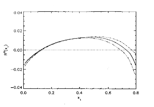
Figure 21: Theoretical estimate of nucleon CSV term $R^{N}_{\pi D}$ of Eq. 74. From Ref. [7].

In Fig. 21 we show the nucleon CSV contribution, $R^{N}_{\pi D}(x)$, using the bag model predictions for CSV, evolved to $Q^{2}=10$ GeV². As the main uncertainty in our calculation is the mean diquark mass, the results are shown for several values of this parameter. In the region $0.4\leq x\leq 0.7$, we predict $R^{N}$ will always be positive, with a maximum value of about 1.7%.

We predict that the contributions from pion and nucleon CSV will all be the same sign and will add constructively.

Since the Drell-Yan ratios arising from CSV are expected to be very small, even small contributions from sea quarks could make a substantial effect. The dominant contribution will arise from interference between one sea quark and one valence quark. We concluded that for sufficiently large $x$, e.g. $x\geq 0.4$, one should be able to separate the CSV “signal” from the sea-valence interference [7]. Unlike the CSV contributions of Eq. (74), the sea-valence interference term $R^{SV}_{\pi D}(x,x_{\pi})$ does not separate, so one could exploit the very different dependence on $x$ and $x_{\pi}$ of the background and CSV terms. We conclude that the CSV terms could be extracted even in the presence of a sea-valence “background”.

Despite our prediction in Sect. 3 that the fractional “minority quark” CSV term, $\delta d(x)/d_{\rm v}(x)$, should be between 3 and 7% (c.f. Fig. 10), the nucleonic CSV ratio $R^{N}_{\pi D}$, shown in Fig. 21, is predicted to be more like 1-2%. This is because $\delta d$ in Eq. (74) is divided by $u^{p}+d^{p}$, and at large $x$ $d^{p}(x)<<u^{p}(x)$. A much larger ratio could in principle be obtained by comparing the $\pi^{+}-p$ and “$\pi^{-}-n$” Drell-Yan processes through the ratio :

$$R^{DY}_{\pi N}(x,x_{\pi})=\frac{4\sigma_{\pi^{+}p}^{DY}(x,x_{\pi})+\sigma_{\pi^{-}p}^{DY}(x,x_{\pi})-\sigma_{\pi^{-}D}^{DY}(x,x_{\pi})}{\left(4\sigma_{\pi^{+}p}^{DY}(x,x_{\pi})-\sigma_{\pi^{-}p}^{DY}(x,x_{\pi})+\sigma_{\pi^{-}D}^{DY}(x,x_{\pi})\right)/2}.$$ (75)

In principle, the advantage of this measurement is that it isolates the minority quark CSV term – in fact, the dominant term in Eq. 75 is the term $\delta d_{\rm v}(x)/d_{\rm v}(x)$ so we expect CSV effects at the 3-7 % level.

We conclude, however, that this quantity is unlikely to provide unambiguous information regarding parton charge symmetry violation. First, to form the ratio in Eq. 75 one must know the relative normalization of DY cross sections on protons and deuterons. This should be feasible by bombarding both hydrogen and deuterium targets simultaneously with charged pion beams. In order to extract the minority quark CSV term, it is necessary to know the precise relation between deuteron parton distributions and those for free nucleons. If we include “EMC” changes in the deuteron structure functions relative to free proton and neutron distributions, we find that 2-3% changes in the parton distributions can produce 10-30% changes in the ratios of Eq. 75. In view of the sensitivity of this ratio to the EMC term, we conclude that information regarding CSV effects could not be extracted from comparing DY cross sections for $\pi^{-}p$ with those for “$\pi^{+}-n$” unless the Fermi motion and binding corrections for the deuteron were known to great accuracy.

Comparing the Drell-Yan yield for $\pi^{+}$ and $\pi^{-}$ on deuterons may provide a means to extract the charge symmetry violating [CSV] part of the nucleon parton distribution. As the $x$ and $x_{\pi}$ values of interest for the proposed measurements are large ($x>0.5$), a beam of 40-50 GeV pions will produce sufficiently massive dilepton pairs that the Drell-Yan mechanism is applicable. A flux of more than $10^{9}$ pions/sec. is desirable, so these experiments might be feasible when the new FNAL Main Injector becomes operable.

5.3 Charged Pion Leptoproduction from Isoscalar Targets

In a recent paper [81], we pointed out that semi-inclusive pion production, from lepton DIS on nuclear targets, could also be a sensitive probe of CSV effects in the valence parton distributions for the nucleon.

In the quark/parton model, the semi-inclusive production of hadrons in deep inelastic lepton scattering from a nucleon is given by

$${1\over\sigma_{N}(x)}{d\sigma^{h}_{N}(x,z)\over dz}={N^{Nh}(x,z)\over\sum_{i}e^{2}_{i}q^{N}_{i}(x)}.$$ (76)

The quantity $N^{Nh}$ in Eq. (76), the yield of hadron $h$ per scattering from nucleon $N$, has the form $N^{Nh}\equiv\sum_{i}e^{2}_{i}q^{N}_{i}(x)D^{h}_{i}(z)$, where $D^{h}_{i}(z)$ is the fragmentation function for a quark of flavor $i$ into hadron $h$, which depends on the quark longitudinal momentum fraction $z=E_{h}/\nu$, where $E_{h}$ and $\nu$ are the energy of the hadron and the virtual photon respectively.

For pion electroproduction on an isoscalar target, (such as the deuteron) charge symmetry relates the “favored” production of charged pions from valence quarks, by

$$N^{D\pi^{+}}_{fav}(x,z) = 4\,N^{D\pi^{-}}_{fav}(x,z).$$ (77)

In Eq. 77, $N^{D\pi^{+}}_{fav}(x,z)$ represents the yield of $\pi^{+}$ per scattering from the deuteron, via the “favored” mode of production, e.g., for $\pi^{+}$ ($\pi^{-}$) production, the “favored” mode of charged pion production is from the target up (down) quarks. Since the semi-inclusive reactions are proportional to the square of the quark charge, there is a relative weighting of 4 for $\pi^{+}$ production.

Deviations from Eq. 77 will arise from effects due to sea quarks, CSV effects in the parton distributions, and contributions from the “unfavored” fragmentation functions. The HERMES collaboration at HERA [82] is currently taking experimental data on semi-inclusive pion production from hydrogen and deuterium .

Assuming charge conjugation invariance and charge symmetry for the fragmentation functions allows us to write the yield for leptoproduction of a charged pion from a proton as

$$N^{p\pi^{\pm}}(x,z) = D^{\pi^{\pm}}_{u}(z)\left[{4\over 9}u^{p}(x)+{1\over 9}\bar{d}^{p}(x)\right]+D^{\pi^{\mp}}_{u}(z)\left[{4\over 9}\bar{u}^{p}(x)++{1\over 9}d^{p}(x)\right]$$ (78)

$$+ {1\over 9}D^{\pm}_{s}(z)\left[s^{p}(x)+\bar{s}^{p}(x)\right]~{}~{}.$$

The fragmentation functions have been extracted by the EMC group [83, 84], and are being independently measured by the HERMES collaboration [82].

We proposed measuring the quantity $\widetilde{R}^{D}(x,z)$, defined by

$$\widetilde{R}^{D}(x,z) \equiv {1-\Delta(z)\over 1+\Delta(z)}\left[{4\,N^{D\pi^{-}}(x,z)-N^{D\pi^{+}}(x,z)\over N^{D\pi^{+}}(x,z)-N^{D\pi^{-}}(x,z)}\right]$$ (79)

$$\approx {5\Delta(z)\over 1+\Delta(z)}+{4\left[\delta d(x)-\delta u(x)\right]\over 3\,\left[u^{p}_{\rm v}(x)+d^{p}_{\rm v}(x)\right]}$$

$$+ {5\left(\bar{u}^{p}(x)+\bar{d}^{p}(x)\right)+\Delta_{s}(z)\left[s(x)+\bar{s}(x)\right]/(1+\Delta(z))\over\left[u^{p}_{\rm v}(x)+d^{p}_{\rm v}(x)\right]}\quad.$$

In Eq. (79), we expand to first order in “small” quantities. These are: the CSV nucleon terms, $\delta d(x)$ and $\delta u(x)$, and the sea quark distributions (Eq. (79) is only valid at large $x$ where the ratio of sea/valence quark distributions is small). We have neglected the CSV part of the fragmentation function; in Ref. [81] we estimated that this term would be quite small.

The quantity $\widetilde{R}^{D}(x,z)$ in Eq. 79 separates into three pieces. The first piece depends only on $z$. This term is a function only of the experimentally measured quantity $\Delta(z)$, the unfavored/favored ratio of fragmentation functions. It decreases roughly monotonically as $z$ increases. The second term depends only on $x$, and is proportional to the nucleon CSV fraction (relative to the valence quark distributions). The final term in Eq. 79 depends on both $x$ and $z$. It is proportional to the sea quark contributions, so it becomes progressively less important at large $x$. It also contains a term which is proportional to the strange/favored ratio of fragmentation functions $\Delta_{s}(z)$: we estimate that this term is always negligible.

Experimentally, one needs to measure accurately the $x$-dependence of $\widetilde{R}^{D}(x,z)$ for fixed $z$; in this case the $z$-dependent term will be large (of order one) and constant. The sea quark contribution will be large at small $x$, but should fall off monotonically and rapidly with $x$. So, at sufficiently large $x$, the sea quark contribution will be negligible relative to the CSV term. One then has to extract the small, $x$-dependent term in Eq. (79) from the large term independent of $x$. As a general rule, the larger the values of $x$ and $z$ at which data can be taken, the larger the CSV term will be relative to the $z$-dependent term.

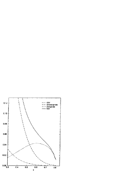
Figure 22: $x$-dependent contributions to charged pion leptoproduction, from Ref. [81].

In Fig. 22 we plot our predictions for the $x$-dependent terms in $\widetilde{R}^{D}(x,z)$, at $Q^{2}=10$ GeV². The long dashed curve is the contribution from nonstrange sea quarks to $\widetilde{R}^{D}_{sea}(x,z)$. This depends only on $x$, and is calculated using the CTEQ3M parton distributions [85]. The short dashed curve is our prediction for the parton charge symmetry violating term, $\widetilde{R}^{D}_{CSV}(x)$; this uses the CTEQ3M parton distributions, plus the bag model prediction for valence quark CSV from Londergan et al. [7], as discussed in Sect. 3. The dot-dashed curve is our estimate of the strange quark contribution. The solid curve is the sum of the three terms.

For $x\approx 0.5$, the CSV term is as large as the sea quark contribution, and with increasing $x$ (e.g., for $x\geq 0.55$), the CSV term dominates the $x$ dependent terms. We predict the maximum CSV contribution will be of order $0.02-0.04$. The $x$ dependent contribution shown in Fig. 22 will sit on a large and constant $z$ dependent term. This term is predicted to vary between 1.5 and 1, as $z$ goes from 0.4 to 0.8 [81]. So the CSV term is expected to be between 1-4% of the $z$-dependent term.

In the HERMES experiment at HERA, the goal is to make precision measurements of the spin structure functions, so the prospect for obtaining very accurate spin-averaged charged pion leptoproduction data is excellent. Only data from deuterium targets is required; efficient detection of both signs of charged pions is important, but absolute yields are not required as overall normalizations cancel out in the ratio of Eq. (79).

6 Charge Symmetry and Flavor Symmetry Contributions to Sum Rules

Sum rules can provide extremely useful information on parton distributions. For example, from the quark model the integrals of up and down valence quark distributions obey the quark number sum rules, given by the normalization conditions on the quark distributions, see Eq. 22 in Sect. 2.

Two sum rules, the Adler sum rule [86] and Gross-Llewellyn Smith sum rule [87], can be directly related to linear combinations of quark normalization integrals. The Adler sum rule is obtained by integrating the difference between the $F_{2}$ structure functions for charged-current interactions of antineutrinos on protons, and that for neutrinos on protons. The Gross-Llewellyn Smith sum rule is obtained by summing the $F_{3}$ structure functions for charged current interactions of neutrinos, and antineutrinos, on a proton target (the same result is obtained for a neutron target).

The Gottfried sum rule (GSR) [3] is obtained by integrating the difference between the $F_{2}$ structure functions for (photon mediated) neutral current interactions on protons and neutrons. Unlike the Adler or Gross-Llewellyn Smith sum rules, the “naive” Gottfried sum rule expectation $S_{G}=1/3$ is obtained only if we assume both charge symmetry for parton distributions, and what is frequently called “SU(2) flavor symmetry” in the proton sea. That is, in addition to charge symmetry we assume that $\bar{u}^{p}(x)=\bar{d}^{p}(x)$.

There has been much recent interest in the Gottfried sum rule, sparked by the rather precise measurements of the NMC group [4]. These show rather conclusively that $S_{G}$ is substantially less than 1/3. If charge symmetry is valid, this provides information on SU(2) flavor symmetry violation [FSV] in the proton sea. In fact, the level of FSV needed to agree with the NMC result is surprisingly large. However, as we will see, the experimental GSR measurements are actually sensitive to a combination of FSV and CSV in the nucleon sea.

As we have argued in this paper, we would expect CSV effects in parton distributions to be no greater than about one percent for sea quark distributions, and for the “majority” valence quark distribution. However, we expect the “minority” valence quark distribution to exhibit CSV effects of several percent at large $x$. As we discussed in Sect. 4, the current experimental upper limits on CSV are of the order of a few percent for $0.1\leq x\leq 0.4$; upper limits for CSV are no better than 10% for larger values of $x$, and for $x<0.1$ the best experiments to date suggest a violation of parton charge symmetry. It would therefore be useful to construct sum rules which could in principle distinguish between CSV and FSV effects. In this Section, we will review the Adler, Gross-Llewellyn Smith and Gottfried sum rules, clarifying the various assumptions implicit in their derivation (particularly the role of charge symmetry in the sum rules). Next, we will propose sum rules which can clearly differentiate between charge symmetry violation and flavor symmetry violation in nucleon sea quark distributions. Finally, we will present existing deep inelastic structure functions in the context of these new sum rules, to examine the degree to which existing data can constrain limits on charge symmetry and/or flavor symmetry violating effects.

The discussion of new sum rules follows rather closely the prior theoretical work of Ma [16, 17]. The sum rules we introduce are linear combinations of those proposed by Ma. He also pointed out the potential confusion in the literature on the question of charge symmetry.

We first review existing sum rules (Gottfried, Gross-Llewellyn Smith, Adler) without making the usual assumptions of charge symmetry in quark distributions. The NMC measurements of the Gottfried Sum Rule [4] are seen as strongly suggesting large flavor symmetry violation [FSV] in the proton sea quark distributions. The Drell-Yan measurements carried out by the NA51 [14] and E866 [15] groups are regarded as more or less definitive proof of large FSV effects. We point out that all three results could in principle be explained by large charge symmetry violation in the nucleon sea quark parton distributions (alternatively, a linear combination of FSV and CSV effects could be responsible for these results).

In Sect. 7, we introduce “flavor symmetry” and “charge symmetry” sum rules, and discuss how they can separate CSV and FSV effects in nucleon sea quark distributions. We discuss what (if any) experimental limits on CSV and FSV can be drawn from existing deep inelastic neutrino scattering experiments.

6.1 Review of Gottfried Sum Rule

Here we review the Gottfried Sum Rule [3]. We go through this in considerable detail so that the underlying assumptions in its derivation are clear throughout. For a comprehensive review of both experimental and theoretical aspects of the Gottfried Sum Rule, and the related question of the flavor symmetry of the proton sea, see the recent work by Kumano [46].

The Gottfried Sum Rule is given by

$$S_{G} \equiv \int_{0}^{1}\,{dx\over x}\,\left[F_{2}^{\mu p}(x)-F_{2}^{\mu n}(x)\right]\quad.$$ (80)

Because the $F_{2}$ structure function from electron and muon deep inelastic scattering depends on the squared charge of the quarks, the up quark distributions are weighted by a factor of four relative to the down quark distributions.

Rewriting the structure functions in terms of quark distributions, we obtain the result

$$\int_{0}^{1}\,{dx\over x}\left[F_{2}^{\mu p}(x)-F_{2}^{\mu n}(x)\right] = {1\over 9}\int_{0}^{1}\,dx\,\left[4\,u^{p}(x)+4\,\bar{u}^{p}(x)-4\,u^{n}(x)-4\,\bar{u}^{n}(x)\right.$$ (81)

$$+ \left.d^{p}(x)+\bar{d}^{p}(x)-d^{n}(x)-\bar{d}^{n}(x)\right].$$

In obtaining Eq. (81), we assume the strange quark contributions for neutron and proton cancel. We can invoke the “strong” assumption that the strange parton distributions for proton and neutron are identical at each value of $x$, i.e. $s^{p}(x)=s^{n}(x)$ (and similarly for the antiquark distributions); alternatively, we can assume the “weak” condition that the parton distributions need not be identical at all $x$, but that the integrals over $x$ of the appropriate parton distributions are identical for proton and neutron. There is no QCD modification of this sum rule.

Introducing valence quark distributions as in Section 2, i.e. $u_{\rm v}(x)\equiv u(x)-\bar{u}(x)$, we obtain

$$\int_{0}^{1}\,{dx\over x}\left[F_{2}^{\mu p}(x)-F_{2}^{\mu n}(x)\right] = {1\over 9}\int_{0}^{1}\,dx\,\left[4\,u^{p}_{\rm v}(x)+8\,\bar{u}^{p}(x)-4\,u^{n}_{\rm v}(x)\right.$$ (82)

$$- \left.8\,\bar{u}^{n}(x)+d^{p}_{\rm v}(x)+2\,\bar{d}^{p}(x)-d^{n}_{\rm v}(x)-2\,\bar{d}^{n}(x)\right].$$

We now invoke the valence quark normalization conditions, defined in Eq. 22, and we obtain the Gottfried Sum Rule,

$$S_{G} \equiv \int_{0}^{1}\,dx\,\left[{F_{2}^{\mu p}(x)-F_{2}^{\mu n}(x)\over x}\right]$$ (83)

$$= {1\over 3}+{2\over 9}\,\int_{0}^{1}\,dx\,\left[4\,\bar{u}^{p}(x)+\bar{d}^{p}(x)-4\bar{u}^{n}(x)-\bar{d}^{n}(x)\right]\quad.$$

If we make the additional (and customary) “strong” assumption of charge symmetry, e.g.

$$d^{n}(x) = u^{p}(x)$$

$$u^{n}(x) = d^{p}(x)$$

$$\bar{d}^{n}(x) = \bar{u}^{p}(x)$$

$$\bar{u}^{n}(x) = \bar{d}^{p}(x)\quad,$$ (84)

then we obtain the “normal” formulation of the Gottfried Sum Rule [GSR],

$$S_{G}\, {CS\atop=} \,\int_{0}^{1}\,dx\,\left[{F_{2}^{\mu p}(x)-F_{2}^{\mu n}(x)\over x}\right]$$ (85)

$$= {1\over 3}+{2\over 3}\,\int_{0}^{1}\,dx\,\left[\bar{u}^{p}(x)-\bar{d}^{p}(x)\right].$$

Note that the charge symmetric Gottfried Sum Rule, Eq. 85, does not require the “strong” assumption of charge symmetry: it follows also from the “weak” condition that the antiquark distributions are not charge symmetric at all points $x$, but that the integral over all $x$ is the same for, say, the up antiquark distribution in the proton and the down antiquark distribution in the neutron.

With the assumptions we have listed, the Gottfried Sum Rule will be equal to 1/3 if we have SU(2) flavor symmetry in the proton sea, i.e. if $\bar{u}^{p}(x)=\bar{d}^{p}(x)$, or if the integrals over $x$ of these distributions are equal.

One additional point is that the Gottfried “Sum Rule” cannot be obtained from current algebra, that is, the GSR cannot be expressed in terms of equal-time commutators of some observable. The Gottfried Sum Rule is simply a relation which holds in the quark/parton model, with additional assumptions regarding equality of strange and charmed quark expectation values in the proton and neutron. This is not the case for the Adler sum rule, which can be derived either from current algebra relations or the quark/parton model.

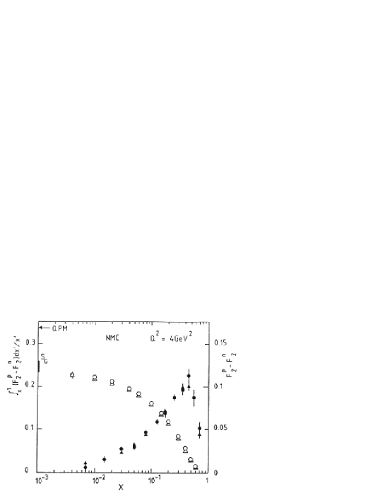
Figure 23: Experimental results for Gottfried sum rule from NMC group, Ref. [4]. Solid dots: $F_{2}^{p}-F_{2}^{n}$; open dots: $\int_{x}^{1}\,[F_{2}^{p}(x^{\prime})-F_{2}^{n}(x^{\prime})]dx^{\prime}/x^{\prime}$.

For almost twenty years there have been indications that the GSR seems to be less than 1/3. However, interest in the Gottfried Sum Rule has intensified with the very accurate measurements in 1991 by the NMC group [4]; the data was re-analyzed in 1994 [45]. Their results are shown in Fig. 23. The solid circles show $F_{2}^{p}(x)-F_{2}^{n}(x)$, while the open circles plot $S_{G}(x)\equiv\int_{x}^{1}[F_{2}^{p}(x)-F_{2}^{n}(x)]\,dx/x$. From Eq. 80 we see that the difference in $F_{2}$ structure functions is multiplied by $1/x$. This means that measurements at low $x$ play a critical role in determining $S_{G}$. Fig. 23 shows that roughly half the contribution to the GSR integral comes from the region $x\leq 0.1$. The neutron results, $F_{2}^{n}$, were inferred from reactions on deuterium.

Earlier measurements by the SLAC, EMC and BCDMS groups [88, 89, 90, 67] gave results which were lower than 1/3, but these values had errors in $S_{G}$ of roughly 20%, so that the results were within one standard deviation of 1/3. The statistical error in the previous experiments was dominated by the lack of data at sufficiently small $x$. The NMC group obtained data for $x$ down to 0.003. The final value from the NMC group was

$$S_{G}(0.004\leq x\leq 0.8)=0.221\pm 0.008~{}(stat)\pm 0.019~{}(syst),$$ (86)

The NMC group then fitted the difference in $F_{2}$ structure functions by a power law and extrapolated from $x=0.004$ to $x=0$ (the extrapolation to $x=1$ produces no measurable contribution to $S_{G}$). Their extrapolated result was

$$S_{G}=0.235\pm 0.026.$$ (87)

This is more than four standard deviations lower than the “naive” expectation of 1/3.

If we use the structure functions for electromagnetic interactions, Eqs. 11 and 28, but do not invoke charge symmetry, we obtain

$$\left[{F_{2}^{\mu p}(x)-F_{2}^{\mu n}(x)\over x}\right] = {1\over 3}\left[u^{p}_{\rm v}(x)-d^{p}_{\rm v}(x)\right]+{2\over 3}\,\left[\bar{u}^{p}(x)-\bar{d}^{p}(x)\right]$$ (88)

$$+ {1\over 9}\,\left[4\delta d(x)+\delta u(x)+4\delta\bar{d}(x)+\delta\bar{u}(x)\right].$$

Integrating this over $x$ and normalizing the valence quarks gives

$$S_{G} = \int_{0}^{1}\,dx\,\left[{F_{2}^{\mu p}(x)-F_{2}^{\mu n}(x)\over x}\right]$$ (89)

$$= {1\over 3}+{2\over 3}\,\int_{0}^{1}\,dx\,\left[\bar{u}^{p}(x)-\bar{d}^{p}(x)\right]$$

$$+ {2\over 9}\,\int_{0}^{1}\,dx\,\left[4\delta\bar{d}(x)+\delta\bar{u}(x)\right].$$

There has been much speculation as to the cause of the NMC result. One possibility is that the Gottfried Sum Rule is, in fact, 1/3, and that the apparent deviation of the GSR from 1/3 is an artifact of the procedure for extrapolating the structure functions to $x=0$. Martin, Roberts and Stirling [12] suggested that one might have $S_{G}=1/3$, where the “missing” contribution to $S_{G}$ comes from very small $x$ values, and that the NMC power law extrapolation was in error.

We discussed in Sect. 4 other theoretical suggestions for the origin of the excess of $\bar{d}^{p}$ over $\bar{u}^{p}$. Recently several groups have compared proton-induced Drell-Yan processes on protons and deuterons. Recent results have been obtained for this process by the NA51 group at CERN [14], and preliminary results from the E866 group at FNAL [15]. Both experiments appear to confirm that $\bar{d}^{p}(x)>\bar{u}^{p}(x)$. This was discussed in more detail in Section 4.

Assuming the NMC extrapolation is correct, from Eq. 89 we see that deviation of the GSR from 1/3 measures either charge symmetry violation [CSV], or flavor symmetry violation [FSV] in the nucleon sea quark distributions (or a combination of the two effects). If we assume the validity of charge symmetry, then the NMC measurement implies a surprisingly large SU(2) flavor asymmetry in the proton antiquark distributions, namely

$$\int_{0}^{1}\,dx\,\left[\bar{d}^{p}(x)-\bar{u}^{p}(x)\right]\ {CS\atop=} \ 0.147\pm 0.039$$ (90)

The FSV contribution suggested by the NMC experiment is surprisingly large, as it is much larger than can be accommodated by perturbative QCD. Both NLO and NNLO QCD calculations have been carried out, and predict very small FSV effects [47]. Consequently, we need a non-perturbative mechanism to generate flavor-violating sea quark distributions which will reproduce the experimental result.

The Pauli principle should make it easier to form a $d\bar{d}$ pair than a $u\bar{u}$ pair in the presence of the valence quarks. In Feynman and Field’s early paper on parton distributions [54], they assumed an excess of $\bar{d}$ quarks in the proton on these grounds. A promising mechanism for generating additional $\bar{d}$ quarks in the proton, first recognized in Ref. [56], is the “Sullivan Effect” [55]. We discussed this briefly in Sect. 4, and refer the interested reader to the review article of Kumano [46].

It is important to note that in principle, one could reproduce the NMC results even if flavor symmetry is exact; this was pointed out by Ma [16]. From Eq. 89, if we assume exact flavor symmetry, but not charge symmetry, in the nucleon sea, then

$$\bar{d}^{p}(x) = \bar{u}^{p}(x)\equiv\bar{q}^{p}(x)$$

$$\bar{d}^{n}(x) = \bar{u}^{n}(x)\equiv\bar{q}^{n}(x)$$

$$\bar{q}^{p}(x) \neq \bar{q}^{n}(x)$$ (91)

then the NMC measurement implies a substantial charge symmetry violation in the nucleon sea, i.e.,

$$\int_{0}^{1}\,dx\,\left[\bar{q}^{p}(x)-\bar{q}^{n}(x)\right]=-0.088\pm 0.023$$ (92)

It would require a very sizable CSV contribution to reproduce the NMC result. The necessary parton sea CSV contribution is more than an order of magnitude larger than the theoretical estimate we discussed in Sect. 3.2. Alternatively, the NMC data could result from a linear combination of FSV and CSV effects in the nucleon sea.

Eq. 92 shows that the Gottfried Sum Rule is sensitive to charge symmetry violation in the nucleon sea. One can also have charge symmetry violation in the valence quark distributions. However, the integral over $x$ of the charge symmetry violating pieces must vanish since CSV contributions cannot change the valence quark normalizations. In principle, violation of charge symmetry in the valence quark distributions makes no contribution to the Gottfried Sum Rule. However, as the valence quark CSV contribution vanishes only when integrated over all $x$, it is possible to obtain a contribution from valence quark CSV if data is taken only over a finite range of $x$. It is important that extrapolations over an unmeasured region properly account for these terms.

6.2 Adler Sum Rule

The Adler Sum Rule is given by the integral of the $F_{2}$ structure functions for charged current neutrino scattering. The Adler Sum Rule, $S_{A}$, can be defined as

$$S_{A} \equiv \lim_{Q^{2}\rightarrow\infty}\,\int_{0}^{1}\,dx\,\left[{F_{2}^{W^{-}p}(x,Q^{2})-F_{2}^{W^{+}p}(x,Q^{2})\over 2x}\right]$$ (93)

$$= \int_{0}^{1}\,dx\,\left[u^{p}(x)-\bar{u}^{p}(x)-\left(d^{p}(x)-\bar{d}^{p}(x)\right)\left(1-|V_{td}|^{2}\right)-s(x)+\bar{s}(x)\right]$$

$$= 1\quad.$$

We obtain the result $S_{A}=1$ if we neglect the term $|V_{td}|^{2}\approx 1\times 10^{-4}$. The Adler sum rule thus requires measuring the $F_{2}$ structure function for antineutrinos and neutrinos on protons, dividing by $x$ (which emphasizes the contribution from very small $x$), and subtracting them. The Adler sum rule then follows from the normalization of the quark distributions. As a consequence of the algebra of SU(2) charges, the Adler sum rule has no QCD corrections.

Figure 24: Experimental results for Adler sum rule, Eq. 93 from the WA25 group, Ref. [73].

In Fig. 24 we show the experimental situation regarding the Adler sum rule. The experimental data are from the WA25 experiment [73], using the CERN-SPS wide band neutrino and antineutrino beams in the BEBC H and D bubble chambers. The experimental data are shown for several values of $Q^{2}$. The average value is $S_{A}=1.01\pm 0.08\pm 0.18$. However, as pointed out by Sterman et al. [21], the total $\nu N$ cross section used by the WA25 group is smaller than the presently accepted value [91, 92]. If the WA25 value is readjusted to fit this total cross section their result becomes $S_{A}=1.08\pm 0.08\pm 0.18$.

Within the rather large errors, the results are independent of $Q^{2}$. The large errors arise from the factor $1/x$ in the integral, Eq. 93. This gives a heavy weighting to the data at small $x$. The paucity of data in this region and the relatively large error bars there give a large uncertainty in the sum rule value. Because of the difficulties in obtaining sufficient neutrino and antineutrino cross sections at small $x$ values for light nuclear targets, it is unlikely that there will be new experimental neutrino data in the near future which would allow us to test the Adler sum rule.

Note that the experimental points presented involve neutrino measurements on neutrons (e.g., deuterons) and protons, and not antineutrinos and neutrinos on protons, as given in the definition of the Adler sum rule, Eq. 93. This follows from the relation $F_{2}^{W^{+}n}(x,Q^{2})\,{CS\atop=}\,F_{2}^{W^{-}p}(x,Q^{2})$, which follows if one assumes charge symmetry, as was discussed in detail in Section V.A. Thus, the WA25 group does not plot the integral $S_{A}$ of Eq. 93, but instead measures the quantity

$$\widetilde{S}_{A} \equiv \lim_{Q^{2}\rightarrow\infty}\,\int_{0}^{1}\,dx\,\left[{F_{2}^{W^{+}n}(x,Q^{2})-F_{2}^{W^{+}p}(x,Q^{2})\over 2x}\right]$$ (94)

$$= \int_{0}^{1}\,dx\,\left[u^{p}_{\rm v}(x)-d^{p}_{\rm v}(x)-\delta u(x)-\delta\bar{d}(x)\right]$$

$$= 1-\int_{0}^{1}\,dx\,\left[\delta\bar{u}(x)+\delta\bar{d}(x)\right].$$

If charge symmetry is exact, then $S_{A}=\widetilde{S}_{A}$. If we assume that the quark normalization integral is indeed one, then the experimental results allow us to place an upper limit on the integral of the antiquark charge symmetry violating amplitudes at the 20% level. We will discuss this more in Sect. 7.2 in connection with the “charge symmetry” sum rule.

6.3 Gross-Llewellyn-Smith sum rule

The Gross-Llewellyn Smith [GLS] Sum Rule [87] is derived from the $F_{3}$ structure functions for neutrinos and antineutrinos,

$$S_{GLS} \equiv \int_{0}^{1}\,{dx\over 2x}\left[xF_{3}^{W^{+}N_{0}}(x)+xF_{3}^{W^{-}N_{0}}(x)\right]$$ (95)

$$= {1\over 2}\int_{0}^{1}\,{dx\over 2x}\left[xF_{3}^{W^{+}p}(x)+xF_{3}^{W^{-}p}(x)+xF_{3}^{W^{+}n}(x)+xF_{3}^{W^{-}n}(x)\right]$$

$$= {1\over 2}\,\int_{0}^{1}\,dx\,[u^{p}(x)-\bar{u}^{p}(x)+d^{p}(x)-\bar{d}^{p}(x)+c(x)-\bar{c}(x)+s(x)-\bar{s}(x)$$

$$+ u^{n}(x)-\bar{u}^{n}(x)+d^{n}(x)-\bar{d}^{n}(x)+c(x)-\bar{c}(x)+s(x)-\bar{s}(x)]$$

$$= 3\left[\,1-{\alpha_{s}(Q^{2})\over\pi}-a(n_{f})\left({\alpha_{s}(Q^{2})\over\pi}\right)^{2}-b(n_{f})\left({\alpha_{s}(Q^{2})\over\pi}\right)^{3}\right]+\Delta HT\quad,$$

which follows from the normalization of the quark valence distributions. We have presented the sum rule for an isoscalar target. An identical prediction is obtained for either a proton or neutron target, i.e. $xF_{3}^{W^{+}p}(x)+xF_{3}^{W^{-}p}(x)$ or $xF_{3}^{W^{+}n}(x)+xF_{3}^{W^{-}n}(x)$, in the integrand of the sum rule. Neither the Adler nor Gross-Llewellyn Smith sum rules require any additional assumptions regarding charge symmetry of quark distributions. The GLS sum rule does, however, acquire a QCD correction, which is represented by the term in square brackets in Eq. 95. The higher order QCD corrections have been derived by Larin and Vermarseren [93]. They depend on the strong coupling $\alpha_{s}(Q^{2})$. The terms $a$ and $b$ depend on the number of quark flavors ($n_{f}$) available at a particular value of $Q^{2}$. The quantity $\Delta HT$ represents a higher twist contribution [94].

As is the case for the Adler and Gottfried sum rules, the Gross-Llewellyn Smith sum rule requires that the structure function be divided by $x$ in performing the integral. This gives a strong weighting to the small-$x$ region, such that as much as 90% of the sum rule comes from the region $x\leq 0.1$. The GLS sum rule is the most precisely known of the three sum rules we consider. The best (and most recent) value has been obtained by the CCFR collaboration [95], which measured neutrino and antineutrino cross sections on iron targets, using the quadrupole triplet beam (QTB) at FNAL. In Fig. 25 we show the CCFR measurements, the experimental values of $xF_{3}$, and their integral, vs. $x$. They obtain cross sections at several values of $x$ and $Q^{2}$; the final value for the sum rule is given for $Q^{2}=3$ GeV². Their reported value for the sum rule is $S_{GLS}=2.50\pm 0.018\pm 0.078$. The GLS sum rule is therefore known to 3%.

Figure 25: Experimental results for Gross-Llewellyn Smith sum rule, Eq. 95, from CCFR group, Ref. [95].

A theoretical value for the Gross-Llewellyn Smith sum rule requires evaluating the QCD corrections. The most recent calculations include next-to-leading order QCD corrections. They use a QCD scale parameter $\Lambda_{QCD}=213\pm 50$ MeV. With this scale parameter and NLO QCD corrections, one obtains a theoretical prediction $S_{GLS}=2.63\pm 0.04$. The theoretical prediction is just within two standard deviations of the experimental value. In Fig. 26 we show the evolution over time of the GLS sum rule value.

Figure 26: Experimental results for Gross-Llewellyn Smith sum rule, and their errors, for a series of experiments, in chronological order from top to bottom.

The errors on the GLS sum rule are now at a level where the value of the strong coupling constant $\alpha_{s}$ is a major source of error. The CCFR group may now have data on $xF_{3}$ over a wide enough range of $Q^{2}$ that, together with renormalized data from several other experiments, they may be able to evaluate the GLS sum rule without extrapolation for a large range of $Q^{2}$ values. This raises the hope that one can calculate the Gross-Llewellyn Smith sum rule as a function of $Q^{2}$, and to use the resulting $Q^{2}$ dependence of the sum rule to determine $\alpha_{s}(Q^{2})$.

The CCFR group has recently re-calculated both the GLS sum rule, and the strong coupling constant $\alpha_{s}$ [96]. With data of this quality over a large $Q^{2}$ range, it may be possible to use the $Q^{2}$ dependence to put constraints on the strong coupling constant. Additional information regarding this procedure can be found in the thesis by Seligman [70].

The quantities $xF_{3}^{W^{+}N_{0}}(x)+xF_{3}^{W^{-}N_{0}}(x)$, which form the integrand for the GLS sum rule, are obtained by taking the difference between cross sections for neutrinos and antineutrinos on isoscalar targets. This was discussed in Sect. 2.5. If charge symmetry is exact, then the $F_{2}$ structure functions exactly cancel when we take the difference of neutrino and antineutrino cross sections, and we are left only with the $F_{3}$ structure functions. However, if we allow charge symmetry violation, then insofar as the sum of $F_{3}$ structure functions is defined as the difference between neutrino and antineutrino cross sections on an isoscalar target, there are additional contributions to this integrand, i.e. using Eqs. 29 and 35,

$${3\pi\over 2G^{2}M_{N}E}\left(d\sigma^{\nu N_{0}}/dx-d\sigma^{\bar{\nu}N_{0}}/dx\right) = {1\over 2}\left(xF_{3}^{W^{+}N_{0}}(x,Q^{2})+xF_{3}^{W^{-}N_{0}}(x,Q^{2})\right)$$ (96)

$$+ F_{2}^{W^{+}N_{0}}(x,Q^{2})-F_{2}^{W^{-}N_{0}}(x,Q^{2})$$

$$= {x\over 2}\left[2\left(u^{p}_{\rm v}(x)+d^{p}_{\rm v}(x)\right)+6\left(s(x)-\bar{s}(x)\right)\right.$$

$$- \left.3\delta u_{\rm v}(x)+\delta d_{\rm v}(x)\right]$$

In addition to the valence quark distributions which we obtain in the charge symmetric limit, there is an additional contribution of three times the difference between strange and antistrange quarks. There is an additional term proportional to the valence quark CSV terms. From Sect. 3, the CSV terms are predicted to have opposite signs so their contributions should add coherently in Eq. 96. Although we expect charge symmetry violating contributions of at most about two percent in the $F_{2}$ structure functions, the relative contribution to the experimental values of $F_{3}$ could be somewhat larger. This is because in the double differential neutrino cross sections (see, e.g., Eq. 7), the $F_{3}$ structure functions are multiplied by a coefficient $y-y^{2}/2$, while $F_{2}$ has a coefficient which is roughly 1. Since the average value of $y$ in these experiments is about 0.2, the $F_{2}$ structure functions will on average be weighted by a factor 5 relative to the $F_{3}$ terms. Thus, naively we expect CSV effects in $F_{2}$ to be magnified by a factor of about 5 in extracting $F_{3}$. Thus a 2% CSV amplitude in the quark distributions could potentially change the extracted value of $F_{3}$ by as much as 10%.

Despite the possibility that the $F_{3}$ structure functions could be modified by quark CSV effects, in principle, these CSV amplitudes should have no effect on the GLS sum rule. Since the GLS sum rule involves an integral over $x$, the net contribution to the sum rule arising from the CSV effects is

$$\delta S_{GLS}^{CSV}=\int_{0}^{1}\,dx\left[\delta d_{\rm v}(x)-\delta u_{\rm v}(x)\right]=0$$ (97)

The integral vanishes because the quark valence distributions obey the normalization conditions, Eq. 22. Therefore the integral over $x$ of both $\delta d_{\rm v}(x)$ and $\delta u_{\rm v}(x)$ must be exactly zero. In practice, this requires having data over all $x$, or correctly performing an extrapolation over the unmeasured $x$ region, so that the contributions from valence quark CSV terms really average to zero.

7 Flavor Symmetry and Charge Symmetry Sum Rules

From the previous section, we see that both FSV and CSV terms contribute to the Gottfried sum rule, and that what is conventionally called the “Adler sum rule” also contains a CSV contribution from sea quarks. If sufficiently accurate experimental data can be obtained, it would be useful to derive sum rules which could differentiate between charge symmetry and flavor symmetry violation in the nucleon sea. Quantities like the electromagnetic interactions, and Drell-Yan processes, which couple to virtual photons are proportional to the squares of the quark charges. They will give the up quark (and antiquark) distributions a relative weighting four times that for the down quark distributions. Neutrino deep inelastic structure functions, which couple to the weak isospin, allows the possibility of separating these contributions.

This process of defining sum rules which would differentiate between charge symmetry and flavor symmetry violation was originally carried out by Ma [16]. Our charge symmetry and flavor symmetry sum rules are linear combinations of the integrals defined by Ma.

7.1 Charge symmetry sum rule

We define a “charge symmetry” sum rule in terms of the $F_{2}$ structure functions for charged current neutrino interactions on the neutron and proton,

$$S_{CS} \equiv \lim_{Q^{2}\rightarrow\infty}\,\int_{0}^{1}\,{dx\over 2x}\,\left[F_{2}^{W^{-}p}(x)-F_{2}^{W^{+}n}(x)\right]$$ (98)

$$= \int_{0}^{1}\,dx\,\left[u^{p}(x)+\bar{s}(x)+\bar{d}^{p}(x)-\left(d^{n}(x)+s(x)+\bar{u}^{n}(x)\right)\right]$$

$$= \int_{0}^{1}\,dx\,\left[\delta u(x)+\delta\bar{d}(x)+\bar{s}(x)-s(x)\right]=\int_{0}^{1}\,dx\,\left[\delta\bar{u}(x)+\delta\bar{d}(x)\right].$$

In deriving $S_{CS}$, we assume that the strange and charmed contributions for neutron and proton are identical. We term this the “charge symmetry” sum rule, since by inspection if either the strong form or weak form of charge symmetry holds for the nucleon sea quark distributions, then $S_{CS}$ will be identically equal to zero, and any deviation from zero will be due to violation of charge symmetry. (To reiterate, the “strong form” of charge symmetry for sea quarks is the statement that $\bar{u}^{p}(x)=\bar{d}^{n}(x)$ for all $x$; the “weak form” would state that the distributions might not be identical, but that their integrals over $x$ are equal. With either form of charge symmetry, the contribution to the integrals in the sum rule would vanish). Just as for the Adler sum rule, there are no QCD corrections to the charge symmetry sum rule.

We can relate the charge symmetry sum rule to the sum rules listed in Sect. 6.2. We can easily see that

$$S_{CS} = S_{A}-\widetilde{S}_{A}\quad\quad{\rm where}$$

$$S_{A} = \lim_{Q^{2}\rightarrow\infty}\,\int_{0}^{1}\,dx\,\left[{F_{2}^{W^{-}p}(x,Q^{2})-F_{2}^{W^{+}p}(x,Q^{2})\over 2x}\right],$$

$$\widetilde{S}_{A} = \lim_{Q^{2}\rightarrow\infty}\,\int_{0}^{1}\,dx\,\left[{F_{2}^{W^{+}n}(x,Q^{2})-F_{2}^{W^{+}p}(x,Q^{2})\over 2x}\right]$$ (99)

The Adler sum rule $S_{A}$ requires comparing the structure function $F_{2}$ for charged current weak interactions on protons with antineutrino beams, and with neutrino beams. We discussed this at length in Sect. 6.2 (see Eq. 94). It is required to be one from normalization of valence quark distributions, and has no contribution from CSV terms.

The sum rule $\widetilde{S}_{A}$ requires subtracting the corresponding $F_{2}$ structure functions for neutrinos on neutrons (i.e., deuterons) and protons, respectively; neutrino beams on different targets. The “charge symmetry” sum rule requires comparing antineutrinos on protons, with neutrinos on neutrons. As an alternative to the charge symmetry sum rule one could measure $S_{A}$ and $\widetilde{S}_{A}$ and compare them. If $S_{A}=1$ and $\widetilde{S}_{A}\neq 1$, this would give clear evidence for charge symmetry violation in the nucleon sea quark distributions.

One can straightforwardly construct sum rules using different linear combinations of $F_{2}$ structure functions for neutrinos or antineutrinos on protons or neutrons, which contain the same information as the sum rules we have defined here. For example, we could define

$$\widetilde{S}_{CS} \equiv \lim_{Q^{2}\rightarrow\infty}\,\int_{0}^{1}\,{dx\over 2x}\,\left[F_{2}^{W^{+}p}(x)-F_{2}^{W^{-}n}(x)\right]$$

$$= \int_{0}^{1}\,dx\,\left[\delta\bar{u}(x)+\delta\bar{d}(x)\right]=S_{CS},\quad\quad{\rm and}$$

$$\widetilde{S}_{A}^{(3)} \equiv \lim_{Q^{2}\rightarrow\infty}\,\int_{0}^{1}\,{dx\over 2x}\,\left[F_{2}^{W^{-}p}(x)-F_{2}^{W^{-}n}(x)\right]=S_{A}+\widetilde{S}_{CS}$$ (100)

$$= 1+\int_{0}^{1}\,dx\,\left[\delta\bar{u}(x)+\delta\bar{d}(x)\right]$$

Experimental prospects for accurate measurements of any of these sum rules are poor. All these sum rules require precision measurements for both neutrinos and antineutrinos, over a wide range of $x$. Since the sum rules are very sensitive to the small $x$ region, it is important to have precise data down to very small $x$. Furthermore, all the sum rules require data on both hydrogen and deuterium targets. As the WA25 group [73] measured cross sections from both neutrinos and antineutrinos on protons and deuterium, they could in principle construct the charge symmetry sum rule. However, as we have seen (viz., Fig. 24 of Section 6.2), the errors in the Adler sum rule are of the order of 20%, so the charge symmetry sum rule would be consistent with zero at the 20% level. We discussed in the previous section the difficulties in obtaining precise neutrino data on light targets, over a wide range of $x$.

We can compare our “charge symmetry” sum rule with the one proposed by Ma [16]. He defined the following sum rule (Eq. [14] of Ref. [16])

$$S_{CS}^{(Ma)} \equiv \,\int_{0}^{1}\,{dx\over 2x}\,\left[F_{2}^{W^{+}p}(x)+F_{2}^{W^{-}p}(x)-\left(F_{2}^{W^{+}n}(x)+F_{2}^{W^{-}n}(x)\right)\right]\quad.$$ (101)

We see that if the charge symmetry sum rule can be written as $S_{CS}^{(Ma)}=S_{CS}+\widetilde{S}_{CS}$; and since we have shown that $S_{CS}=\widetilde{S}_{CS}$, all three of these sum rules give precisely the same information.

7.2 Flavor symmetry sum rule

We can define a “flavor symmetry” sum rule by comparing the $F_{3}$ structure functions from charged current neutrino interactions on protons and neutrons, i.e.

$$S_{FS} \equiv \,\int_{0}^{1}\,{dx\over 2x}\,\left[xF_{3}^{W^{+}n}(x)-xF_{3}^{W^{+}p}(x)\right]$$ (102)

$$= \,\int_{0}^{1}\,dx[-\left(\bar{u}^{p}(x)+\bar{c}(x)-d^{p}(x)-s(x)\right)$$

$$+ d^{n}(x)+s(x)-\bar{u}^{n}(x)-\bar{c}(x)]$$

$$= \int_{0}^{1}\,dx\,\left[d_{\rm v}^{n}(x)-d_{\rm v}^{p}(x)+\bar{u}^{p}(x)-\bar{u}^{n}(x)-\bar{d}^{p}(x)+\bar{d}^{n}(x)\right]$$

$$= \left(1+\int_{0}^{1}\,dx\,\left[\bar{u}^{p}(x)-\bar{d}^{p}(x)-\bar{u}^{n}(x)+\bar{d}^{n}(x)\right]\right)\left(1-{\alpha_{s}(Q^{2})\over\pi}\right).$$

If flavor symmetry holds for the nucleon sea, i.e. if $\bar{u}^{p}(x)=\bar{d}^{p}(x)$ and $\bar{u}^{n}(x)=\bar{d}^{n}(x)$ (or the weak condition that the integrals over $x$ of these distributions are equal), then $S_{FS}$ will be equal to one. So any deviation of this sum rule from one signifies flavor symmetry violation in the nucleon sea. There is a QCD correction to this sum rule. It is the same as for the Gross-Llewellyn Smith sum rule (see Section 6.3). In Eq. 102 we include the lowest-order QCD correction.

Experiments with muons suggest the magnitude of flavor symmetry breaking which we might expect. As we discussed in Sect. 3.2, theoretical calculations predict that sea quark CSV effects will be very small. In that case the antiquark contributions to Eq. 102 will be identical to those measured by the NMC group [4]. For $Q^{2}=10$ GeV², we then expect the integral over the antiquark distributions to give a 30% effect. However, there will be significant experimental difficulties obtaining accurate data for the sum rule. The factor $1/x$ in the integrand requires precise neutrino data on both protons and neutrons (i.e., deuterium), at very small $x$. Even small differences between the $F_{3}$ structure functions on protons and deuterium become magnified when one integrates the difference between them.

Our flavor symmetry sum rule was obtained by combining $F_{3}$ structure functions for neutrinos on protons and neutrons. We could define an analogous function by utilizing antineutrino structure functions on protons and neutrons,

$$\bar{S}_{FS} \equiv \,\int_{0}^{1}\,{dx\over 2x}\,\left[xF_{3}^{W^{-}p}(x)-xF_{3}^{W^{-}n}(x)\right]$$ (103)

$$= \int_{0}^{1}\,dx\,\left[u_{\rm v}^{p}(x)-u_{\rm v}^{n}(x)+\bar{u}^{p}(x)-\bar{u}^{n}(x)-\bar{d}^{p}(x)+\bar{d}^{n}(x)\right]$$

$$= \left(1+\int_{0}^{1}\,dx\,\left[\bar{u}^{p}(x)-\bar{d}^{p}(x)-\bar{u}^{n}(x)+\bar{d}^{n}(x)\right]\right)\left(1-{\alpha_{s}(Q^{2})\over\pi}\right)\quad.$$

Comparing Eq. 103 with Eq. 102 we see that $\bar{S}_{FS}=S_{FS}$; consequently both of these sum rules give exactly the same information.

Ma defines an additional sum rule, $S^{\prime}$ (Eq. [23] of Ref. [16]), through

$$S^{\prime} \equiv \,\int_{0}^{1}\,{dx\over x}\left[xF_{3}^{W^{+}p}(x)-xF_{3}^{W^{-}p}(x)-xF_{3}^{W^{+}n}(x)+xF_{3}^{W^{-}n}(x)\right]$$ (104)

$$= \left(-4-4\int_{0}^{1}\,dx\,\left[\bar{u}^{p}(x)-\bar{d}^{p}(x)-\bar{u}^{n}(x)+\bar{d}^{n}(x)\right]\right)\left(1-{\alpha_{s}(Q^{2})\over\pi}\right).$$

This is related to the two previously defined sum rules by $S^{\prime}=-2(S_{FS}+\bar{S}_{FS})$, and gives the same information as either of those. It requires knowledge of both neutrino and antineutrino parity violating structure functions on both the proton and neutron.

8 Conclusions

We have reviewed the validity of charge symmetry for parton distributions. We calculated CSV contributions for both valence and sea quarks. The “majority” valence quark distribution, and the sea quark distribution, are predicted to obey charge symmetry to at least 1% for all values of $x$. The “minority” valence quark distribution, however, is predicted to show CSV effects of between 3-7% at large Bjorken $x$. This prediction appears to be robust, as all calculations of quark CSV predict effects of this magnitude, and reasonably model-independent estimates confirm these results.

This violation of charge symmetry is large. If this turns out to be correct, we should probably re-evaluate all phenomenological parton distributions, introduce some explicit charge symmetry violation and re-fit existing cross sections. Towards this end, we have redefined a number of observables, using a formalism which does not assume explicit parton charge symmetry. One difficulty in searching for CSV effects at present is that all phenomenological parton distributions assume charge symmetry at the outset, so any existing CSV effects have been absorbed into the current parton distributions. This makes it difficult to search for experimental violation of charge symmetry. Of course, if CSV effects were extremely large, we would already have seen this in existing experimental data.

If charge symmetry is indeed violated at the predicted level for the minority valence quarks, then one should be able to measure such effects. First, we reviewed the status of current tests of parton charge symmetry. There are essentially two such tests. The first involves the comparison of charge-current cross sections induced by neutrinos to those from antineutrinos. This comparison can detect CSV in valence quark distributions; the test is only valid at large $x$. Existing data gives only weak upper limits on valence quark CSV. The second test of parton CSV is the so-called “charge ratio,” the ratio of $F_{2}$ structure functions in DIS processes induced by leptons, to the $F_{2}$ structure functions in charge-changing weak processes from neutrino beams (both of these need to be measured on isoscalar targets). Despite the fact that this comparison requires a large number of corrections, it appears that most of these corrections are under control.

Recent data, muon induced DIS on deuterium from the NMC group [4], and neutrino reactions on iron from the CCFR group at FNAL [65], allow us to place rather tight constraints on parton CSV amplitudes. Such relations should hold at all values of $x$. These experiments allow us to set limits of roughly 10% on charge symmetry violating contributions to parton distributions, in the region $0.2\leq x\leq 0.4$. However, in the region $x<0.2$, there appears to be a discrepancy between the electromagnetic and weak $F_{2}$ structure functions.

In this review, we have suggested several experiments specifically designed either to detect CSV in parton distributions, or to set more stringent upper limits on parton CSV. Probably the most sensitive test would be a comparison of the $F_{2}$ structure functions for charge-changing weak processes induced by electrons and positrons on an isoscalar target. At sufficiently high energies (such as are accessible at HERA), comparison of $e^{+}-D$ and $e^{-}-D$ processes should be a powerful and relatively clean test of parton CSV. Other potentially useful reactions which are quite sensitive to parton CSV are Drell-Yan processes for charged pions on isoscalar nuclear targets, or semi-inclusive leptoproduction of pions on isoscalar targets. We made estimates of the magnitude of CSV effects expected in these reactions.

We also discussed the contributions of CSV effects in various sum rules. We showed that CSV contributions to the nucleon sea have no effect on the Gross-Llewellyn Smith sum rule, but in principle they affect both the Adler and Gottfried sum rules. In fact, the existing experimental “test” of the Adler sum rule contains a contribution from CSV in sea quark distributions, and can be used to place an upper limit on parton sea quark CSV. We introduced two new sum rules, a “charge symmetry” sum rule which is zero if charge symmetry is exact, and a “flavor symmetry” sum rule which is one if flavor symmetry is exact in the nucleon sea. Both sum rules require measuring the structure functions for neutrinos and/or antineutrinos on isoscalar targets, with particular attention to the small-$x$ region. Limits on CSV from present experiments are in the neighborhood of 10% of the average parton distributions.

Acknowledgments

This review includes research supported in part by the US National Science Foundation under research contract NSF-PHY-9722076, and by the Australian Research Council. One author [JTL] would also like to thank the Special Research Centre for the Subatomic Structure of Matter for its hospitality during a period when this review was written. The authors acknowledge several discussions with A. Pang regarding sections of this review. In addition, the authors would like to acknowledge discussions with and contributions by C. Benesh, C. Boros, S. Braendler, G.T. Garvey, R.L. Jaffe, G.Q. Liu, W. Melnitchouk and E.N. Rodionov. One author [JTL] acknowledges several discussions with S. Kumano, and wishes to thank C. Keslin and D. Murdock for assistance with the figures for this review.

References

- [1] G. A. Miller, B. M. K. Nefkens and I. Slaus, Phys. Rep. 194 (1990) 1.
- [2] E. M. Henley and G. A. Miller in Mesons in Nuclei, eds. M. Rho and D. H. Wilkinson (North-Holland, Amsterdam 1979).
- [3] K. Gottfried, Phys. Rev. Lett. 18 (1967) 1174.
- [4] P. Amaudruz et al (NMC Collaboration), Phys. Rev. Lett. 66 (1991) 2712; Phys. Lett. B295 (1992) 159.
- [5] G. Preparata, P. G. Ratcliffe and J. Soffer, Phys. Rev. Lett. 66 (1991) 687.
- [6] E. M. Henley and G. A. Miller, Phys. Lett. B 251 (1990) 453.
- [7] J. T. Londergan, G. T. Garvey, G. Q. Liu, E. N. Rodionov and A. W. Thomas, Phys. Lett. B 340 (1994) 115.
- [8] J. T. Londergan, G. Q. Liu, E. N. Rodionov and A. W. Thomas, Phys. Lett. B 361 (1995) 110.
- [9] J. Levelt, P. J. Mulders and A. W. Schreiber, Phys. Lett. B 263 (1991) 498.
- [10] L. Frankfurt et al, Phys. Lett. B 230 (1989) 141.
- [11] S. Kumano and J. T. Londergan, Phys. Rev. D 44 (1991) 717; Phys. Rev. D 46 (1992) 457.
- [12] A.D.Martin,W.J.Stirling and R.G.Roberts, Phys. Lett.B252 (1990) 653.
- [13] S.D.Ellis and W.J.Stirling, Phys. Lett. B256 (1991) 258.
- [14] A. Baldit et al. (NA51 collaboration), Phys. Lett. B332 (1994) 244.
- [15] E866 Collaboration, P.E. Reimer et al., Proceedings of Sixth Conference on the Intersections Between Particle and Nuclear Physics, (American Inst. of Physics, 1997) 643.
- [16] B.-Q. Ma, Phys. Lett. B 274 (1992) 111.
- [17] B.-Q. Ma, A. Schäfer and W. Greiner, Phys. Rev. D 47 (1993) 51.
- [18] E. Sather, Phys. Lett. B 274 (1992) 433.
- [19] E. N. Rodionov, A. W. Thomas and J. T. Londergan, Int. J. Mod. Phys. Letts. A 9 (1994) 1799.
- [20] E.Leader and E.Predazzi, An Introduction to Gauge theories and Modern Particle Physics, (Cambridge University Press, Cambridge, 1996).
- [21] George Sterman et al., Rev. Mod. Phys. 67 (1995) 157.
- [22] V.N. Gribov and L.N. Lipatov, Sov. J. Nucl. Phys. 15 (1972) 438; G. Altarelli and G. Parisi, Nucl. Phys.B126 (1977) 298.
- [23] C.G. Callan and D.G. Gross, Phys. Rev. Lett. 22 (1969) 156.
- [24] L.W. Whitlow et al, Phys. Lett. B250 (1990) 193.
- [25] H. Georgi and H.D. Politzer, Phys. Rev. D14 (1976) 1829; R.M. Barnett, Physica (Amsterdam) 14D (1976) 70.
- [26] For criticism of the “slow rescaling” model, and concerns about extracting the strange quark distributions from measurements made near charm threshold, see the papers by Barone et al., ref. [27].
- [27] V. Barone, M. Genovese, N.N. Nikolaev, E. Predazzi and B.G. Zahkarov, hep-ph 9505343; Phys. Lett. B317 (1993) 433; Phys. Lett. B328 (1994) 143.
- [28] C. Foudas et al. (CCFR Collaboration), Phys. Rev. Lett. 64 (1990) 1207.
- [29] S.A. Rabinowitz et al. (CCFR Collaboration), Phys. Rev. Lett. 70 (1993) 134.
- [30] A.O. Bazarko et al. (CCFR Collaboration), Z. Phys. C65 (1995) 189.
- [31] M. Glück, S. Kretzer and E. Reya, Phys. Lett. B380 (1996) 171.
- [32] A.I. Signal and A.W. Thomas, Phys. Lett. B191 (1987) 206.
- [33] X. Ji and J. Tang, Phys. Lett. B362 (1995) 182.
- [34] H. Holtmann, A. Szczurek and J. Speth, Nucl. Phys. A596 (1996) 631.
- [35] S.J. Brodsky and B.-Q. Ma, Phys. Lett. B381 (1996) 317.
- [36] W. Melnitchouk and W. Malheiro, Phys. Rev. C55 (1997) 431.
- [37] C.J. Benesh and T. Goldman, Phys. Rev. C55 (1997) 441.
- [38] A. I. Signal and A. W. Thomas, Phys. Rev. D 40 (1989) 2832; A. W. Schreiber et al., Phys. Rev. D 44 (1991) 2653.
- [39] A.W.Schreiber,A.W.Thomas and J.T.Londergan, Phys. Rev. D42 (1990) 2226.
- [40] W. Melnitchouk, A. W. Schreiber and A. W. Thomas, Phys. Rev.D49 (1994) 1183.
- [41] A. Chodos et al. Phys. Rev.D10 (1974) 2599.
- [42] E. Naar and C. Birse, Phys. Lett.B305 (1993) 190.
- [43] F.E.Close and A.W.Thomas, Phys. Lett. B212 (1988) 227.
- [44] C.J. Benesh and J. T. Londergan, Second International Workshop on Symmetries in Physics, Seattle, WA, June 1997, (unpublished).
- [45] M. Arneodo et al (NMC Collaboration), Phys. Rev. D50 (1994) R1.
- [46] S. Kumano, to be published, Phys. Rept. (preprint hep-ph/9702367).
- [47] D.A. Ross and C.T. Sachrajda, Nucl. Phys. B149 (1979) 497.
- [48] S.D. Drell and T.M. Yan, Phys. Rev. Lett. 25 (1970) 316; Ann. Phys. (NY) 66 (1971) 578.
- [49] D. M. Alde et al. (E772 Collaboration), Phys. Rev. Lett.64 (1990) 2479.
- [50] H.L. Lai et al. (CTEQ Collaboration), Phys. Rev. D55 (1997) 1280.
- [51] A.D. Martin, R.G. Roberts and W.J. Stirling, Phys. Rev. D50 (1994) 6734; Phys. Lett. B354 (1995) 155.
- [52] M. Glück, E. Reya and A. Vogt, Z. Phys. C67 (1995) 433.
- [53] F. Steffens and A.W. Thomas, Phys. Rev. C55 (1997) 900.
- [54] R. D. Field and R. P. Feynman, Nucl. Phys. B 136 (1978) 1.
- [55] J.D. Sullivan, Phys. Rev. D5 (1972) 1732.
- [56] A.W. Thomas, Phys. Lett. B126 (1983) 97.
- [57] J. Speth and A.W. Thomas, “Mesonic Contributions to the Spin and Flavor Structure of the Nucleon,” (Juelich preprint, to be published in Advances in Nuclear Physics, 1997).
- [58] A. Szczurek and J. Speth, Nucl. Phys. A555 (1993) 249; A. Szczurek et al., Nucl. Phys. A596 (1996) 397.
- [59] E.J. Eichten, I. Hinchliffe and C. Quigg, Phys. Rev. D45 (1992) 2269.
- [60] S.J. Dong and K.F. Liu, Phys. Lett. B328 (1994) 130.
- [61] E.V. Shuryak and J.J.M. Verbaarschot, Nucl. Phys. B410 (1993) 55.
- [62] T. Schaefer, E.V. Shuryak and J.J.M. Verbaarschot, Nucl. Phys. B412 (1994) 143.
- [63] P.D. Meyers et al., Phys. Rev. C34 (1986) 1265.
- [64] D.B. MacFarlane et al. (CCFRR Collaboration), Z. Phys. C26 (1984) 1.
- [65] W.G. Seligman et al., Phys. Rev. Lett. 79 (1997) 1213.
- [66] A.C. Benvenuti et al. (BCDMS Collaboration), Phys. Lett. B237 (1990) 592.
- [67] A.C. Benvenuti et al. (BCDMS Collaboration), Phys. Lett. B195 (1987) 91.
- [68] L.W. Whitlow, Ph. D. thesis, Stanford University, preprint SLAC-357 (1990).
- [69] C. Boros, A.W. Thomas and J.T. Londergan, to be published, 1998.
- [70] W.G. Seligman, Ph.D. thesis, Columbia University, 1997; publ. CU-398, Nevis-292. This can be accessed via the URL www.nevis.columbia.edu/pub/ccfr/seligman.
- [71] A. Donnachie and P.V. Landshoff, Z. Phys. C61 (1994) 139.
- [72] Q. Zhu, for the ZEUS Collaboration, Proceedings of DIS96 Conference, Rome (1996).
- [73] D. Allasia et al. (WA25 Collaboration), Phys. Lett. B135 (1984) 231; Z. Phys. C28 (1985) 321.
- [74] J.T. Londergan, S.M. Braendler and A.W. Thomas, to be published, Phys. Lett. B (preprint hep-ph/9708459)..
- [75] Y. Nambu and G. Jona-Lasinio, Phys. Rev.122 (1961) 345; ibid. 124 (1961) 246.
- [76] T. Shigetani, K. Suzuki and H. Toki, Phys. Lett.B308 (1993) 383.
- [77] T. Shigetani, K. Suzuki and H. Toki, Tokyo Metropolitan University preprint: TMU-NT940101 (1994).
- [78] A. Bodek and J. L. Ritchie, Phys. Rev.D23 (1981) 1070.
- [79] L. L. Frankfurt and M. I. Strikman, Phys. Rep.160 (1988) 235.
- [80] R. P. Bickerstaff and A. W. Thomas, J. Phys.G15 (1989) 1523.
- [81] J.T. Londergan, Alex Pang and A.W. Thomas, Phys. Rev. D54 (1996) 3154.
- [82] G. van der Steenhoven, Workshop on Future Physics at HERA May 1996, p. 1022 (DESY Library).
- [83] J. J. Aubert et. al. (EMC Collaboration), Phys. Lett. B160 (1985) 417.
- [84] M. Arneodo et. al. (EMC Collaboration), Nucl. Phys. B321 (1989) 541.
- [85] H. L. Lai et. al. (CTEQ collaboration), Phys. Rev. D51 (1995) 4763.
- [86] S.L. Adler, Phys. Rev. 143 (1966) 1144.
- [87] D.J. Gross and C.H. Llewellyn Smith, Nucl. Phys. B14 (1969) 337.
- [88] L.W. Whitlow et al., Phys. Lett. B282 (1992) 475.
- [89] S. Dasu et al., Phys. Rev. Lett. 61 (1988) 1061.
- [90] J. Ashman et al. (EMC Collaboration), Phys. Lett.B206 (1988) 364; Nucl. Phys.B328 (1990) 1.
- [91] R. Blair et al., Phys. Rev. Lett. . 51 (1983) 343.
- [92] P. Berge et al., Z. Phys. C35 (1987) 443.
- [93] S.A. Larin and J.A.M. Vermarseren, Phys. Lett. B259 (1991) 345.
- [94] V.M. Braun and A.V. Kolesnichenko, Nucl. Phys. B283 (1987) 723.
- [95] W.C. Leung et al. (CCFR Collaboration), Phys. Lett. B317 (1993) 655.
- [96] D.A. Harris et al. (CCFR Collaboration), conf proceedings [hep-ex/9506010].
- [97] H. Abramowitz et al. (CDHS Collaboration), Z. Phys. C17 (1983) 283.
- [98] A.Signal,A.W.Schreiber and A.W.Thomas, Mod. Phys. Lett. A6 (1991) 271.
- [99] S.Kumano, Phys. Rev. D43 (1991) 59.
- [100] W.Melnitchouk and A.W.Thomas, Phys. Rev. D47 (1993) 3783; V.R.Zoller, Phys. Lett. B279 (1992) 145; B.Badelek and J.Kwiecinski, Nucl. Phys. B370 (1991) 278.
- [101] W.Melnitchouk,A.W.Thomas and A.I.Signal, Zeit. Phys. 340 (1991) 85.