Abstract

We make a model–independent analysis of all available data that indicate neutrino oscillations. Using probability diagrams, we confirm that a mass spectrum with two nearly degenerate pairs of neutrinos separated by a mass gap of $\simeq 1$ eV is preferred over a spectrum with one mass eigenstate separated from the others. We derive some new relations among the four–neutrino mixing matrix elements. We design four-neutrino mass matrices with three active neutrinos and one sterile neutrino that naturally incorporate maximal oscillations of atmospheric $\nu_{\mu}$ and explain the solar neutrino and LSND results. The models allow either a large or small angle MSW or vacuum oscillation description of the solar neutrino deficit. The models predict (i) oscillations of either $\nu_{e}\rightarrow\nu_{\tau}$ or $\nu_{e}\rightarrow\nu_{s}$ in long–baseline experiments at $L/E\gg 1$ km/GeV, with amplitude determined by the LSND oscillation amplitude and argument given by the atmospheric $\delta m^{2}$, and (ii) the equality of the $\nu_{e}$ disappearance probability, the $\nu_{\mu}$ disappearance probability, and the LSND $\nu_{\mu}\rightarrow\nu_{e}$ appearance probability in short–baseline experiments.

1 Introduction

The long–standing solar neutrino deficit [1, 2], the atmospheric neutrino anomaly [3, 4, 5, 6], and the results from the LSND experiment on ${\bar{\nu}}_{e}$ neutrinos from $\mu^{+}$ decay and $\nu_{e}$ neutrinos from $\pi^{+}$ decay [7] can each be understood in terms of oscillations between two neutrino species [8]. Interestingly, the solar, atmospheric, and terrestrial (LSND) neutrino oscillations have different $L/E$ and therefore require different neutrino mass–squared differences $\delta m^{2}$ to properly describe all features of the data. For example, if the atmospheric and LSND $\delta m^{2}$ scales are the same [9], one forfeits the recently reported zenith-angle dependence and up/down asymmetry of the atmospheric neutrino flux [4, 5]. Alternatively, if the solar and atmospheric $\delta m^{2}$ scales [10] are the same, the reduction in the solar neutrino flux is energy-independent, contrary to the three solar experiments which infer different oscillation probabilities in different neutrino energy regions [11]. Since three distinct mass-squared differences cannot be constructed from just three neutrino masses, the collective data thus argue provocatively for more than three oscillating flavors. An alternative but less compelling possibility is to introduce new lepton–flavor changing operators with coefficients small enough to evade present exclusion limits, but large enough to explain the small LSND amplitude [12].

If all of the existing observations are confirmed, a viable solution is to invoke one or more additional species of sterile light neutrino [13], thereby introducing another independent mass scale to the theory. The additional neutrino must be sterile, i.e. without Standard Model gauge interactions, to be consistent with LEP measurements of $Z\rightarrow\nu\bar{\nu}$ [14]. The introduction of a sterile neutrino to complement the three active neutrinos has had some phenomenological success [15].

In this paper we propose and study mass matrices for four–neutrino models (three active plus one sterile) that can accommodate all the present data. Once a fourth neutrino is admitted to the spectrum, it is no longer mandatory that the $\nu_{\mu}$ mix with the $\nu_{\tau}$ at the atmospheric scale. The $\nu_{\mu}$ may instead mix with the sterile $\nu_{s}$, or with some linear combination of $\nu_{s}$ and $\nu_{\tau}$. Similarly, the $\nu_{e}$ may mix with a linear combination of $\nu_{s}$ and $\nu_{\tau}$.

At first sight the mixing of a sterile neutrino with active flavor neutrinos seems to be stringently constrained by Big Bang nucleosynthesis (BBN) physics. The bound

$$\delta m^{2}\sin^{2}2\theta<10^{-7}{\rm~{}eV}^{2}$$ (1)

on the mass-squared difference $\delta m^{2}$ and the mixing angle of the sterile neutrino was inferred to avoid thermal overpopulation of the “extra” sterile neutrino species[16]. However, there are significant caveats to this bound. One is the fact that some recent estimates of $N_{\nu}$ using higher abundances of ⁴He yield considerably weaker bounds [17]. Another is that a small asymmetry $(n_{\nu}-n_{\bar{\nu}})/n_{\gamma}\mathrel{\raisebox{-2.58334pt}{$\stackrel{{\scriptstyle\textstyle>}}{{\sim}}$}}7\times 10^{-5}$ of flavor neutrinos (but large compared to the present baryon asymmetry $\Delta n_{B}/n_{\gamma}\sim 10^{-10}$) at $t>0.1$ s is enough to suppress $\nu_{\mu}-\nu_{s}$ oscillations and then the bound of Eq. (1) does not apply [18]. Such asymmetries, in fact, can be generated with the kind of model parameters considered herein (as shown in Ref. [19, 20]). In light of this observation that BBN may allow sizeable mixing between sterile and active neutrinos, we consider both the small and large mixing with sterile neutrinos in this work.

We review all existing data that indicate neutrino oscillations, and then perform a model–independent analysis of the data using four–neutrino unitarity constraints. A very useful tool for this unitarity analysis is the set of probability rectangles, which we explain and exploit. We draw several model–independent conclusions for the four–neutrino universe.

We design a five–parameter neutrino mass matrix which can account for each of the three viable solar solutions and accommodate the atmospheric and LSND observations. The three solar possibilities are the small-angle matter-enhanced (SAM) [21, 22, 23, 24], large-angle matter enhanced (LAM) [25] and large–angle vacuum long–wavelength (VLW) [26, 27] explanations of the solar neutrino deficit. Our mass matrix yields maximal oscillations of atmospheric $\nu_{\mu}$. We consider the possibility that the solar data is explained by $\nu_{e}\rightarrow\nu_{s}$ or $\nu_{e}\rightarrow\nu_{\tau}$ oscillations, in which case the atmospheric neutrino data is explained by either $\nu_{\mu}\rightarrow\nu_{\tau}$ or $\nu_{\mu}\rightarrow\nu_{s}$ oscillations, respectively. We also consider the possibility that both atmospheric and solar neutrino oscillations have $\nu_{s}$ and $\nu_{\tau}$ components. Lack of $\nu_{s}$–$\nu_{\tau}$ discrimination in the present data is the major source of ambiguity in the four–neutrino model. We discuss how future experiments can resolve this ambiguity.

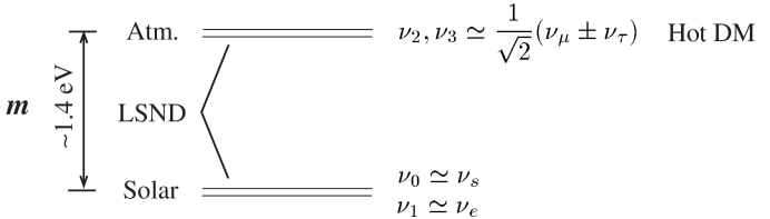
Figure 1: Neutrino mass spectrum, showing a possible flavor assignment for each mass eigenstate, and showing which mass splittings are responsible for the LSND, atmospheric, and solar oscillations.

In Sec. 2 we summarize the oscillation probability formulas and utilize a probability formalism, based on unitarity of the mixing matrix, which permits a simple visual represention of mixing. In Sec. 3 we begin with a brief discussion of the three classes of experiments and the neutrino mass and mixing parameters needed to explain them. We then use probability rectangles to display the inferences from the data for any four–neutrino scheme. In Sec. 4 we employ the probability rectangles to argue against a neutrino mass spectrum with one eigenstate separated from three other nearly–degenerate states (which we will refer to as the 1+3 spectrum) in favor of two nearly degenerate mass pairs (which we will refer to as the 2+2 spectrum). We also derive some new relations among elements of the mixing matrix that result from data and unitarity which are satisfied in a four–neutrino model for certain ranges of the parameters. Then in Sec. 5 we present a mass matrix whose eigenvalues consist of a nearly degenerate neutrino pair at $\sim 1.4$ eV and another nearly degenerate pair at low mass, as illustrated in Fig. 1. We show how the existing data almost uniquely fixes the model parameters (once a solar scenario is specified) and strictly determines what new phenomenology the model predicts. In Sec. 6 we derive expressions for the oscillation probabilities in our models in terms of the current neutrino experimental observables. We present the model predictions in Sec. 7. The new observable signature for the model is $\nu_{e}\leftrightarrow\nu_{\tau}$ or $\nu_{e}\leftrightarrow\nu_{s}$ oscillations for $L/E\gg 1$ km/GeV, depending on whether the atmospheric oscillations are $\nu_{\mu}\rightarrow\nu_{\tau}$ or $\nu_{\mu}\rightarrow\nu_{s}$, respectively. Section 8 contains some discussion, and a summary.

2 Formalism

2.1 Oscillation amplitudes

To simplify the analysis of the available data, we will ignore possible CP violation and work with a real–valued mixing matrix $U$. Accordingly, the general formula for the vacuum oscillation probabilities becomes [28]

$$P(\nu_{\alpha}\to\nu_{\beta})=\delta_{\alpha\beta}-4\sum_{k<j}U_{\alpha k}U_{\beta k}U_{\alpha j}U_{\beta j}\sin^{2}\Delta_{jk}\,,$$ (2)

where $\Delta_{jk}\equiv\delta m_{jk}^{2}\,L/4E=1.27(\delta m^{2}_{jk}/{\rm eV}^{2})(L/{\rm km})/(E/{\rm GeV})$, $\delta m^{2}_{jk}\equiv m^{2}_{j}-m^{2}_{k}$, and the sum is over all $j$ and $k$ subject to $k<j$.

For oscillations of two neutrinos, the oscillation amplitude (i.e., the coefficient of the $\sin^{2}\Delta_{jk}$ term) is given by $\sin^{2}2\theta$, where $\theta$ is the mixing angle between the two neutrino states. More generally for an arbitrary number of neutrinos, the amplitude of the $\nu_{\alpha}$ to $\nu_{\beta}$ oscillation in the absence of CP violation is seen to be

$$A^{\alpha\beta}=-4\sum_{k<j}U_{\alpha j}U_{\beta j}U_{\alpha k}U_{\beta k}\,,\qquad\alpha\neq\beta\,,$$ (3)

where the sum is over mass states with mass-squared differences appropriate for the $L/E$ of the particular experiment. We note that the oscillation amplitudes defined here are only for those oscillations at a particular $\Delta$ scale in Eq. (2). We will use subscript labels on the amplitude to identify the $\Delta$ scale (which is determined by the relevant $\delta m^{2}$ and $L/E$) for the particular experiment: “sbl” will denote short–baseline experiments such as LSND, “atm” will denote atmospheric and long–baseline experiments, and “sun” will denote extraterrestrial experiments, especially those with solar neutrinos.

We will use superscripts on the amplitude to identify the oscillation flavors, unless it is obvious from the context; in the absence of CP violation, $A^{\alpha\beta}=A^{\beta\alpha}$. With four neutrino states, $U$ is a $4\times 4$ mixing matrix. We also define the amplitude for $\nu_{\alpha}$ disappearance

$$A^{\alpha\not\alpha}\equiv\sum_{\beta\neq\alpha}A^{\alpha\beta}\,,$$ (4)

where ${\not\alpha}$ represents a sum over neutrino flavor eigenstates other than $\nu_{\alpha}$. The mixing–matrix elements $U$, and therefore the amplitudes $A$, depend on the environment, e.g., matter vs. vacuum. Throughout this paper we will quote values for the oscillation amplitudes in vacuum.

2.2 Probability rectangles and a theorem

The “probability rectangles” used by Liu and Smirnov [20] visually illustrate the mixing of the flavor eigenstates among the mass eigenstates. To construct the probability rectangles, we introduce the notation

$$P_{\alpha j}\equiv|U_{\alpha j}|^{2},$$ (5)

such that $P_{\alpha j}$ is the probability that the $\alpha^{th}$ flavor state is found in the $j^{th}$ mass state, or, alternatively, the probability that the $j^{th}$ mass state is contained in the $\alpha^{th}$ flavor state. Therefore, when CP–violation is neglected, the real mixing–matrix elements are determined by the probabilities up to a sign: $U_{\alpha j}=\pm\sqrt{P_{\alpha j}}$. In principle, these signs may be determined by arranging for orthogonality of the rows, and columns, in the unitary mixing matrix $U$.

By unitarity of $U$ we have

$$\sum_{\alpha}P_{\alpha j}=1$$ (6)

for each mass state $j$, and

$$\sum_{j}P_{\alpha j}=1$$ (7)

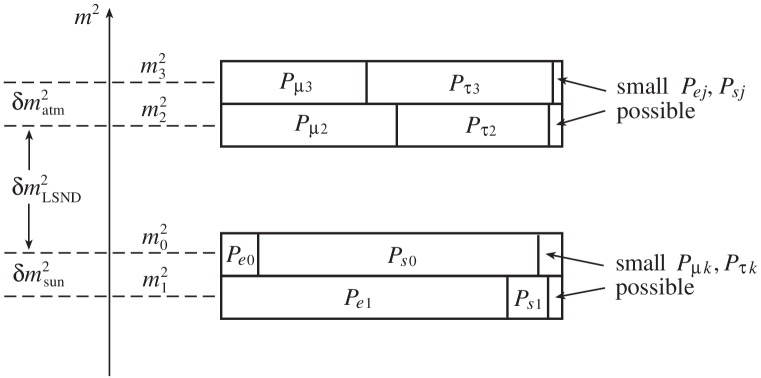
Figure 2: Typical probability rectangles for a 2+2 model where $\nu_{2}$ and $\nu_{3}$ generate the atmospheric oscillations and $\nu_{1}$ and $\nu_{0}$ generate the solar oscillations. For the non-dominant probabilities $j=2$ or $3$ and $k=1$ or $0$.

for each flavor state $\alpha$. Thus, if each mass state is represented as a rectangle of unit area, then the fractional area assigned to $P_{\alpha j}$ within the rectangle is a graphical representation of the value of $P_{\alpha j}$. The probabilities $P_{\alpha j}$ depend on whether the environment is vacuum or matter. For consistency, we will always display vacuum probabilities in the rectangles. When the probability rectangles are displayed along a vertical axis labeled with mass–squared, the $\delta m^{2}$ values relevant for the various experiments are readily visualized. Figure 2 gives an example of the probability rectangles for a four–neutrino model. An inverted 2+2 mass spectrum, where the solar $\nu_{e}$ oscillation is driven by the separation of the heavier two states and the atmospheric $\nu_{\mu}$ oscillation is driven by the separation of the lighter two states, may also be possible, but is not considered.

The following mini-theorem will prove to be useful:
In the absence of matter effects, the amplitude $A^{\alpha\not\alpha}$ is independent of how the $P_{\not\alpha j}$ probabilities are partitioned among the mass eigenstates.
The proof of this statement relies on the insertion of $\sum_{\beta\neq\alpha}U_{\beta j}U_{\beta k}=-U_{\alpha j}U_{\alpha k}$ into
$A^{\alpha\not\alpha}=-4\sum_{\beta\neq\alpha}\sum_{j,k>j}U_{\alpha j}U_{\alpha k}U_{\beta j}U_{\beta k}$, to get

$$A^{\alpha\not\alpha}=4\sum_{j>k}P_{\alpha j}P_{\alpha k},$$ (8)

where, as in Eq. (3), the sum in Eq. (8) is over all mass states with mass-squared differences appropriate for the $L/E$ of the particular experiment. In Eq. (8), $A_{\alpha\not\alpha}$ is manifestly independent of the partitioning of the $P_{\not\alpha j}$ probabilities since it involves only the $P_{\alpha j}$. This theorem demonstrates the limitations on information derivable from disappearance experiments.

The minitheorem fails in the presence of matter effects because the partitioning of the flavor probabilities including $P_{\alpha j}$ are altered. That is, with matter effects the amplitude $A_{\alpha\rightarrow\not\alpha}$ does depend on how the $P_{\not\alpha j}$ are partitioned among the mass states. Matter will also alter the oscillation wavelength, causing further changes in the phenomenology of experiments sensitive to the oscillations rather than their averages. Matter effects have the potential to resolve the $\nu_{s}$–$\nu_{\tau}$ ambiguity, as do some other measurements. We discuss these possibilities in Sec. 7.

3 Experimental constraints

3.1 Short baseline: LSND, reactors, and accelerators

The LSND experiment [7] reports positive appearance results for $\bar{\nu}_{\mu}\rightarrow\bar{\nu}_{e}$ oscillations from $\mu^{+}$ decay at rest (DAR) and for $\nu_{\mu}\rightarrow\nu_{e}$ oscillations from $\pi^{+}$ decay in flight (DIF). The DAR data has higher statistics, but the allowed regions for the two processes are in good agreement. There are also restrictions from the null results of the BNL E-776 [29] and KARMEN [30] $\nu_{\mu}\rightarrow\nu_{e}$ oscillation search experiments. The combined data suggest $\nu_{\mu}\rightarrow\nu_{e}$ vacuum oscillation parameters that lie approximately along the line segment described by

$$0.3{\rm~{}eV}^{2}\leq\delta m^{2}_{sbl}={0.030{\rm~{}eV}^{2}\over(A^{\mu e}_{sbl})^{0.7}}\leq 2.0{\rm~{}eV}^{2}\;.$$ (9)

However, values for $\delta m^{2}_{sbl}$ as high as 10 eV² are also allowed for $A^{\mu e}_{sbl}\simeq.0025$, although values above 3 eV² are disfavored by the r–process mechanism of heavy element nucleosynthesis in supernovae [31].

There are also relevant data from the Bugey reactor experiment which searches for $\bar{\nu}_{e}$ disappearance [32], and from the CDHS[33] and CCFR[34] experiments which set bounds on $\nu_{\mu}$ disappearance.

The combined short baseline data set for $A^{e\not e}$, $A^{\mu\not\mu}$, and $A^{\mu e}$ will be used in Sec. 4 to argue against a hierarchical neutrino mass spectrum in favor of two pairs of nearly degenerate masses in the four–neutrino spectrum.

3.2 Atmospheric data

The atmospheric neutrino experiments measure $\nu_{\mu}$ and $\nu_{e}$ (and their antineutrinos) created when cosmic rays interact with the Earth’s atmosphere. One expects roughly twice as many muon neutrinos as electron neutrinos from the resulting cascade of pion and other meson decays. Several experiments [3, 4] obtain a $\nu_{\mu}/\nu_{e}$ ratio that is about 0.6 of the value expected from detailed theoretical calculations of the flux [35]. The Super-Kamiokande (SuperK) experiment has collected the most data and analysis [4] indicates that their results for contained events can be explained as $\nu_{\mu}\rightarrow\nu_{\tau}$ oscillations with [4, 6, 36]

$$3\times 10^{-4}{\rm~{}eV}^{2}\leq\delta m^{2}_{atm}\leq 7\times 10^{-3}{\rm~{}eV}^{2}\,,\quad 0.8\leq A^{\mu\not\mu}_{atm}\leq 1.0\;.$$ (10)

The high end of each range is favored.

Independent of flux normalization considerations, the $\nu_{\mu}\rightarrow\nu_{e}$ oscillation channel is strongly disfavored by the zenith angle distributions of the data [4] and by the up/down asymmetry separated into “muon–like” ($\nu_{\mu}$) and “electron–like”($\nu_{e}$) events [5], which yield an up–to–down ratio of $0.52^{+0.07}_{-0.06}\pm 0.01$ for $\mu$–like events and $0.84^{+0.14}_{-0.12}\pm 0.02$ for $e$–like events (the expected values are close to unity). Furthermore, the recent CHOOZ $\bar{\nu}_{e}$ disappearance experiment excludes $\bar{\nu}_{e}\rightarrow\bar{\nu}_{\mu}$ oscillations with large mixing $A^{\mu\not\mu}_{atm}\mathrel{\raisebox{-2.58334pt}{$\stackrel{{\scriptstyle\textstyle>}}{{\sim}}$}}0.2$ for $\delta m^{2}_{atm}\geq 10^{-3}{\rm eV}^{2}$ [37].

In a four–neutrino context, another possibility for the atmospheric neutrino oscillations is $\nu_{\mu}\rightarrow\nu_{s}$. Oscillations of this type in principle could be affected by matter due to the different neutral current interactions of $\nu_{\mu}$ and $\nu_{s}$. However, for the contained events (with lower energy) these effects are small, especially for larger values of $\delta m^{2}$ [20, 38]; hence, the allowed regions for $\nu_{\mu}\rightarrow\nu_{s}$ should be similar to those for $\nu_{\mu}\rightarrow\nu_{\tau}$. For events at higher energies the matter effects could begin to be appreciable; a definitive test requires more data.

3.3 Solar data

The solar neutrino experiments [2] measure $\nu_{e}$ created in the sun. There are three types of experiments, $\nu_{e}$ capture in Cl in the Homestake mine, $\nu_{e}-e$ scattering at Kamiokande and Super-Kamiokande, and $\nu_{e}$ capture in Ga at SAGE and GALLEX; each is sensitive to different ranges of the solar neutrino spectrum and measures a suppression from the expectations of the standard solar model (SSM)[1].

For $\nu_{e}\rightarrow\nu_{s}$ oscillations in the sun (in which case atmospheric neutrino oscillations are $\nu_{\mu}\rightarrow\nu_{\tau}$ in our model) the allowed parameter ranges at 95% C.L. [39] for the small-angle matter-enhanced solution are given in Table 1. The solution is based on the SSM fluxes in Ref. [1]. Approximate parameters for the large-angle matter-enhanced [39] and vacuum long–wavelength solutions [40] for $\nu_{e}\rightarrow\nu_{s}$ oscillations of solar neutrinos are also shown in Table 1. If the solar neutrino deficit is caused instead by $\nu_{e}\rightarrow\nu_{\tau}$ oscillations (and the atmospheric oscillations are $\nu_{\mu}\rightarrow\nu_{s}$), then the allowed solar parameter ranges for the three solar cases are slightly different [39]; see Table 1. The exact values of the parameters may change as new data from SuperK [41] become available and when fits are made with the new solar flux calculations.

In any of the matter–enhanced scenarios it is also necessary that the eigenmass $m_{1}$ associated predominantly with $\nu_{e}$ be lighter than the eigenmass $m_{0}$ associated predominantly with the neutrino into which the $\nu_{e}$ is oscillating (i.e., $\nu_{s}$ or $\nu_{\tau}$), so that it is $\nu_{e}$ rather than ${\bar{\nu}}_{e}$ that is resonant in the sun. For the vacuum solutions the ordering of $m_{0}$ and $m_{1}$ does not matter. Alternate scenarios where the $\nu_{e}$ is predominantly associated with the heavier two states and $\nu_{\mu}$ is predominantly associated with the lighter two states are also viable.

For $\nu_{e}\rightarrow\nu_{\tau}$ oscillations in the two-neutrino approximation the propagation equation for the neutrino states in the charge-current basis is [21, 42, 43]

$$i{d\over dt}\left(\begin{array}[]{c}\nu_{e}\\ \nu_{\tau}\end{array}\right)={1\over 4E}\left(\begin{array}[]{cc}4\sqrt{2}G_{F}EN_{e}&\delta m^{2}\sin 2\theta\\ \delta m^{2}\sin 2\theta&2\delta m^{2}\cos 2\theta\end{array}\right)\left(\begin{array}[]{c}\nu_{e}\\ \nu_{\tau}\end{array}\right)\,,$$ (11)

where $N_{e}$ is the electron number density. For $\nu_{e}\rightarrow\nu_{s}$ oscillations the propagation equation is instead [44]

$$i{d\over dt}\left(\begin{array}[]{c}\nu_{e}\\ \nu_{s}\end{array}\right)={1\over 4E}\left(\begin{array}[]{cc}4\sqrt{2}G_{F}E(N_{e}-{1\over 2}N_{n})&\delta m^{2}\sin 2\theta\\ \delta m^{2}\sin 2\theta&2\delta m^{2}\cos 2\theta\end{array}\right)\left(\begin{array}[]{c}\nu_{e}\\ \nu_{s}\end{array}\right)\,,$$ (12)

where $N_{n}$ is the neutron number density. For the small–angle matter–enhanced case the non–adiabatic approximate solution for neutrino propagation is appropriate and the oscillation probability for a neutrino of energy $E_{\nu}$ is

$$P(\nu_{e}\rightarrow\nu_{e})={1\over 2}A^{e\not e}_{sun}+P_{x}(1-A^{e\not e}_{sun})\,$$ (13)

where in this case $\not e$ labels either $\tau$ or $s$, and

$$P_{x}=exp\left[-{\pi\delta m^{2}_{sun}(A_{sun}^{e\not e})^{2}\over 4E_{\nu}\sqrt{1-A^{e\not e}_{sun}}\,(d\log N/dL)_{c}}\right]\,$$ (14)

is the Landau–Zener transition probability and $N$ is either $N_{e}$ (for $\nu_{e}\rightarrow\nu_{\tau}$ oscillations) or $N_{e}-{1\over 2}N_{n}$ (for $\nu_{e}\rightarrow\nu_{s}$ oscillations). The quantity $(d\log N/dL)_{c}$ is the appropriate logarithmic density gradient in the sun at $N^{crit}=\delta m^{2}_{sun}\sqrt{1-A^{e\not e}_{sun}}/(2\sqrt{2}G_{F}E_{\nu})$, the critical density where maximal oscillations (resonance) occur. For the large–angle matter–enhanced case, the neutrino propagation is adiabatic and

$$P(\nu_{e}\rightarrow\nu_{e})={1\over 2}\left[1-\sqrt{1-A^{e\not e}_{sun}}\,\right]\,$$ (15)

assuming the neutrinos are created where the electron density is well above the critical density. For the vacuum long–wavelength solution the oscillation probability is just given by the usual vacuum expressions.

3.4 Oscillation lengths and amplitudes summarized

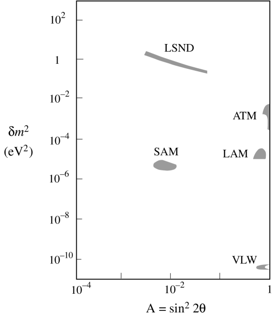
Figure 3: The three allowed two-neutrino solar solutions for $\nu_{e}\rightarrow\nu_{\tau}$ oscillations [45]. The corresponding region for $\nu_{e}\rightarrow\nu_{s}$ oscillations are similar to the $\nu_{e}\rightarrow\nu_{\tau}$ case.

In neutrino oscillation descriptions of the solar, atmospheric, and LSND data, a distinct oscillation wavelength and oscillation amplitude is required for each of the three data sets. Experimental uncertainties allow for some latitude in these amplitudes and wavelengths, and for the solar data, there are three isolated islands of viability in the $\delta m^{2}$–amplitude plane [45]; see Fig. 3. The day–night asymmetry measurement, found to be small in the recent SuperK data, removed about half of the previously viable solar regions [45].

The vacuum oscillation wavelength is linear in the neutrino energy, allowing further possibilities that are summarized in Table 2. The chosen neutrino energies are typical for solar, and reactor sources (5 MeV), pion facilities (100 MeV), for contained (2 GeV), partially–contained (10 GeV), and throughgoing (100 GeV) neutrino events in underground detectors, and for astrophysical sources (1 TeV). Although full oscillation wavelengths are also listed in Table 2, oscillation effects may well be measurable for a fraction of an oscillation wavelength or as an average over many oscillation wavelengths. Throughgoing and partially contained atmospheric neutrinos may show nodes as a function of L/E. Further possibilities arise when the matter effect of the earth is included in the oscillation physics. We consider earth–matter effects in Sec. 7.6.

3.5 Inferences from data

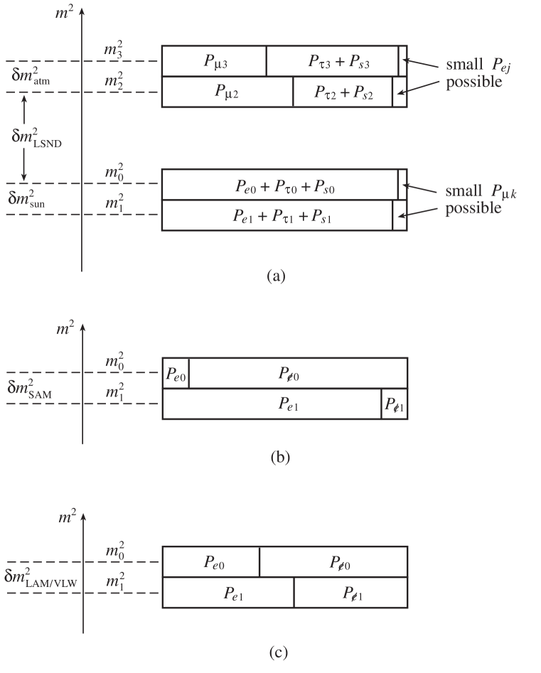
Figure 4: Typical probability rectangles for some 2+2 models. (a) Rectangles deduced from atmospheric and CHOOZ neutrino data, with $\nu_{\mu}$ lying predominantly in the $\nu_{2}$ and $\nu_{3}$ states with large mixing with either $\nu_{\tau}$ and/or $\nu_{s}$. The $P_{\mu 0}$ and $P_{\mu 1}$ probabilites are small, but the $P_{\not\mu 0}$ and $P_{\not\mu 1}$ probabilities are not yet determined. The partitioning of the $P_{\not\mu 0}$ and $P_{\not\mu 1}$ probabilites once the solar solution is specified are also shown for the (b) small angle MSW and (c) large angle MSW or vacuum long–wavelength solutions.

We consider first the probability rectangles for the atmospheric and CHOOZ data. The atmospheric data indicate $\delta m^{2}_{atm}\sim 5\times 10^{-3}$ and nearly maximal flavor–changing mixing of $\nu_{\mu}$ with $\nu_{\not e}$. The present data do not distinguish between $\nu_{\tau}$ or $\nu_{s}$ as the dominant state into which $\nu_{\mu}$ mixes. The probability rectangles for the atmospheric scale are displayed in Fig. 4a. We label the two masses defining the atmospheric scale as $\nu_{2}$ and $\nu_{3}$, with $\delta m^{2}_{atm}=\delta m^{2}_{32}$. Because of the “$\nu_{\tau}$–$\nu_{s}$” ambiguity we show the union $P_{\tau}+P_{s}$ rather than the partitions into $P_{\tau}$ and $P_{s}$. For maximal $\nu_{\mu}$-$\nu_{\not e}$ mixing, one must choose $P_{\mu 2}\sim P_{\mu 3}\sim P_{\tau 2}+P_{s2}\sim P_{\tau 3}+P_{s3}\sim 1/2$.

Next we consider the pair of mass eigenstates whose mass–squared difference is fixed by the solar scale. We provisionally investigate a four–neutrino mass spectrum that consists of two pairs of nearly degenerate neutrinos separated by the LSND scale $\delta m^{2}_{sbl}\sim{\rm eV}^{2}$ (to explain the LSND result in terms of oscillations). We argue in Sec. 4 that the data favor this spectrum over a spectrum with one mass separated from three relatively degenerate masses. We label the second pair of mass states as $\nu_{0}$ and $\nu_{1}$, and define $\delta m^{2}_{sun}=\delta m^{2}_{10}$. Since $P_{\mu 2}$ and $P_{\mu 3}$ sum to near unity, $P_{\mu 0}$ and $P_{\mu 1}$ must be small. Thus the probability rectangles for the $\nu_{0}$ and $\nu_{1}$ states appear as shown in Fig. 4a. Accordingly, the LSND amplitude for $\nu_{\mu}\rightarrow\nu_{e}$,

$$A^{\mu e}_{sbl}=-4\,[U_{\mu 3}U_{e3}+U_{\mu 2}U_{e2}]\,[U_{\mu 1}U_{e1}+U_{\mu 0}U_{e0}]\,,$$ (16)

is necessarily small. We emphasize that the smallness of the LSND $\nu_{e}$–$\nu_{\mu}$ mixing is an inevitable consequence of the large mixing of $\nu_{\mu}$ to $\nu_{\not e}$ at the atmospheric scale and the constraints of unitarity, independent of particular model considerations including rearrangement of the neutrino mass spectrum.

Four–neutrino unitarity may be used to rewrite eqn. (16) as

$$A^{\mu e}_{sbl}=4\,|U_{\mu 3}U_{e3}+U_{\mu 2}U_{e2}|^{2}=4\,|U_{\mu 1}U_{e1}+U_{\mu 0}U_{e0}|^{2}.$$ (17)

Written this way, it is clear that the LSND data is blind to the partitioning of $\nu_{\tau}$ and $\nu_{s}$ in the probability rectangles of mass states $\nu_{0}$ and $\nu_{1}$. This flavor ambiguity is shown in Fig. 4a.

With the identification $\delta m^{2}_{sun}=\delta m^{2}_{10}$, we may use Eq. (8) to write the solar $\nu_{e}$–disappearance amplitude as

$$A^{e\not e}_{sun}=4\,P_{e0}P_{e1}.$$ (18)

Because matter in the sun may exert a significant effect on propagating neutrinos, the values of $P_{e0}$ and $P_{e1}$ for the sun have some sensitivity to the state $\nu_{\tau}$ or $\nu_{s}$ into which $\nu_{e}$ oscillates. However, the sensitivity of present data to this difference is weak, and there is considerable freedom in assigning $\nu_{\tau}$ or $\nu_{s}$ or a linear combination thereof as the mixing partner to $\nu_{e}$. This $\nu_{\tau}$–$\nu_{s}$ ambiguity for $\nu_{e}$ mixing at the solar scale is complementary to the $\nu_{s}$–$\nu_{\tau}$ ambiguity for $\nu_{\mu}$ mixing at the atmospheric scale. Potential measurements to resolve the $\nu_{s}$–$\nu_{\tau}$ ambiguity at the solar scale will be discussed in Sec. 7.

3.6 The three solar solutions

The $P_{e0}$ and $P_{e1}$ partitioning specifies whether the solar model is a small–angle model or a large–angle model. As can be inferred from Eq. (18), with nearly–equal partitioning of $P_{e0}$ and $P_{e1}$, the mixing amplitude is near maximal (large angle). With highly nonequal partitioning, i.e., $P_{e0}\ll P_{e1}$ or $P_{e1}\ll P_{e0}$, the mixing amplitude is small. Of the three viable solar neutrino options, SAM falls into the small angle category, while LAM and VLW fall into the large angle category. The probability rectangles for the small and large angle classes of models are shown in Figs. 4b and 4c. Recall that in order to obtain the MSW resonant enhancement required for the SAM and LAM solutions, it is necessary that the state which is predominantly $\nu_{e}$ be the lighter of the two mass states, $\nu_{1}$. Qualitatively, LAM and VLW are distinguishable in their probability rectangles only by the choice of value for $\delta m^{2}_{sun}$. Quantitatively, the two solutions and the VLW solution are distinguishable in ways which are discussed in Sec. 7.

If the active–sterile mixing is small, then all ambiguities in the probability rectangles are resolved: the large atmospheric mixing must be $\nu_{\mu}$–$\nu_{\tau}$, and the solar solution must be small–angle SAM with $\nu_{e}$–$\nu_{s}$ mixing. The probability rectangles for this model are shown in Fig. 2. This particular solution has recently been analyzed in the context of the minimal four–neutrino mass matrix [46, 47].

4 Mass spectra

4.1 Argument against a 1+3 mass spectrum

It has been shown by Bilenky, Giunti and Grimus [48] that a hierarchical ordering of the four–neutrino spectrum (implying one dominant mass) is disfavored by the data when the null results of reactor and accelerator disappearance experiments are included. We will refer to this spectrum as the 1+3 spectrum, defined as one heavier mass state separated from three lighter, nearly-degenerate states, or vice versa. We demonstrate the argument with a set of logical steps similar to theirs.

Assume a mass spectrum with one heavy mass well separated from three other nearly-degenerate states and let the heavy mass state be labeled as $\nu_{3}$. Then the LSND mass-squared scale is $\delta m^{2}_{sbl}\simeq\delta m^{2}_{32}\simeq\delta m^{2}_{31}\simeq\delta m^{2}_{30}$ and the LSND amplitude is

$$A^{\mu e}_{sbl}=-4\,U_{e3}U_{\mu 3}\,[\sum_{j\neq 3}U_{\mu j}U_{ej}]=4\,P_{e3}P_{\mu 3},\qquad{\rm with~{}}P_{e3}+P_{\mu 3}\leq 1.$$ (19)

On the other hand, the $\nu_{e}$ and $\nu_{\mu}$ disappearance experiments at reactors and accelerators are also sensitive to the LSND scale. These experiments measure the disappearance amplitudes

$$A^{e\not e}_{sbl}=4\,P_{e3}\,[\sum_{j\neq 3}P_{ej}]=4\,P_{e3}\,[1-P_{e3}]$$ (20)

and

$$A^{\mu\not\mu}_{sbl}=4\,P_{\mu 3}\,[1-P_{\mu 3}].$$ (21)

The second equalities in Eqs. (19) and (20) (see Eq. (8)) follow from unitarity of the mixing matrix. The three amplitudes in Eqs. (19)–(21) depend on just two parameters, and so are interrelated. All three of these amplitudes are constrained by experiments to be small. A priori then, $P_{e3}$ and $P_{\mu 3}$ may both be small, or one (but not both) may be near unity with the other small. The fact that $A^{\mu e}_{sbl}$ is an appearance observation rather than a bound means that if $P_{e3}$ and $P_{\mu 3}$ are both small, they cannot be too small.

In the 1+3 model, the atmospheric scale does not involve the heavy state $\nu_{3}$. Without loss of generality we label the state which determines the atmospheric scale as $\nu_{2}$. Then from Eq. (8) the atmospheric $\nu_{\mu}$ disappearance oscillation amplitude is given by

$$A^{\mu\not\mu}_{atm}=4P_{\mu 2}(P_{\mu 0}+P_{\mu 1})\leq(1-P_{\mu 3})^{2}\,,$$ (22)

where the inequality comes from maximizing $4P_{\mu 2}(P_{\mu 0}+P_{\mu 1})$ subject to the constraint $P_{\mu 0}+P_{\mu 1}+P_{\mu 2}=1-P_{\mu 3}$. The SuperK data indicate that $\nu_{\mu}$ is maximally mixed at the $\delta m^{2}_{atm}$ scale, i.e., there is little $\nu_{\mu}$–content available to the $\nu_{3}$ state. Quantitatively we have $A^{\mu\not\mu}_{atm}\geq 0.8$, which implies $P_{\mu 3}\leq 0.11$. Since $P_{\mu 3}$ is small, Eq. (21) becomes

$$A^{\mu\not\mu}_{sbl}\simeq 4\,P_{\mu 3}<<1.$$ (23)

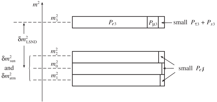
Figure 5: Typical probability rectangles for the 1+3 model when $P_{e3}$ is large and $P_{e\not 3}$ is small.

The probability rectangles for the 1+3 model with small $P_{\mu 3}$ are presented in Fig. 5. Note that it is the zenith–angle, or up/down asymmetry data, which really establishes $\delta m^{2}_{atm}$ as different from $\delta m^{2}_{sbl}$, that is crucial for the argument [48].

We are left with the possibilities of $P_{e3}$ being small or near unity. As can be seen in Fig. 5, if $P_{e3}$ is near unity, then there is little $P_{e\not 3}$ to distribute over the three lighter mass states. In particular, the solar amplitude $A^{e\not e}_{sun}=4P_{e0}P_{e1}$, where the solar scale is $\delta m^{2}_{sun}=\delta m^{2}_{10}$, is second order in small quantities, too small for even the SAM solution ($A_{SAM}\geq 2.5\times 10^{-3}$) to the solar flux. This may be easily quantified. If $P_{e3}$ were near unity, we would have

$$A^{e\not e}_{sbl}\simeq 4\,[1-P_{e3}]<<1.$$ (24)

Together with unitarity, this in turn bounds the magnitude of the solar amplitude:

$$A^{e\not e}_{sun}=4\,P_{e0}P_{e1}\,\leq\,(1-P_{e3})^{2}\simeq\frac{1}{16}(A^{e\not e}_{sbl})^{2},$$ (25)

where the inequality in Eq. (25) comes from maximizing $4P_{e0}P_{e1}$ subject to the constraint $P_{e0}+P_{e1}\leq 1-P_{e3}$. The experimental upper limit on $A^{e\not e}_{sbl}$ from the BUGEY experiment [32] is about 0.1 for $\delta m^{2}_{sbl}\leq 2$ eV², which disallows even the small–angle solar solution. We conclude that $P_{e3}$ is small, in which case

$$A^{e\not e}_{sbl}\simeq 4\,P_{e3}<<1.$$ (26)

Thus, both $P_{e3}$ and $P_{\mu 3}$ must be small in the 1+3 model, and from Eqs. (19), (23), and (26), we infer the relation

$$A^{\mu e}_{sbl}\simeq\frac{1}{4}A^{\mu\not\mu}_{sbl}\;A^{e\not e}_{sbl}.$$ (27)

However, the experimental upper bounds on the disappearance amplitudes $A^{e\not e}_{sbl}$ [32] and $A^{\mu\not\mu}_{sbl}$ [33] and the measured appearance result for $A^{\mu e}_{sbl}$ [7] are not compatible with Eq. (27), thereby disfavoring the 1+3 model. For example, for $\delta m^{2}_{sbl}=0.3$ eV², $A^{e\not e}_{sbl}<0.035$ from Bugey, $A^{\mu\not\mu}_{sbl}<0.8$ from CDHS, which implies $A^{\mu e}_{sbl}<0.007$; however, for this value of $\delta m^{2}_{sbl}$, the LSND data indicate $A^{\mu e}_{sbl}>0.04$. The LSND results are presented in terms of maximum likelihood rather than confidence level limits, so it is not straightforward to state an exclusion probability.

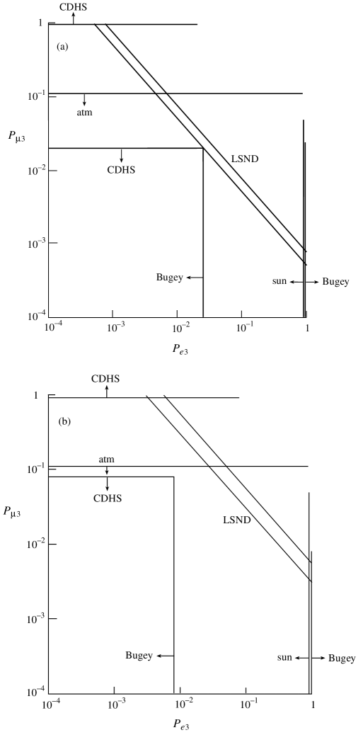
Figure 6: Constraints on $P_{\mu 3}$ and $P_{e3}$ for the 1+3 model when (a) $\delta m^{2}_{sbl}=1.7$ eV² and (b) $\delta m^{2}_{sbl}=0.5$ eV². The LSND, Bugey, CDHS, atmospheric, and solar constraints are obtained by comparison of the appropriate data with Eqs. (19), (20), (21), (22), and (25), respectively. Not displayed is the unitarity constraint $P_{e3}+P_{\mu 3}\leq 1$.

Put another way, $A^{\mu e}_{sbl}$ is large enough that the Bugey and CDHS limits force one of $P_{e3}$ and $P_{\mu 3}$ to be small and the other to be large, but this is ruled out by the solar and atmospheric data. The constraints on $P_{e3}$ and $P_{\mu 3}$ from the three short–baseline amplitudes $A^{e\mu}_{sbl}$, $A^{e\not e}_{sbl}$, and $A^{\mu\not\mu}_{sbl}$, the atmospheric amplitude $A^{\mu\not\mu}_{atm}$ and the solar amplitude $A^{e\not e}_{sun}$ (from Eqs. (19), (20), (21), (22), and (25), respectively) are conveniently summarized in Fig. 6 for two different values of $\delta m^{2}_{sbl}$.

The measured values and bounds for the short–baseline appearance and disappearance amplitudes depend on the magnitude of $\delta m^{2}_{sbl}$. (There is effectively a suppressed $\delta m^{2}_{sbl}$ third axis in our Fig. 6, which samples only two particular values of $\delta m^{2}_{sbl}$.) For certain allowed values of $\delta m^{2}$ (e.g., at 1.7 ${\rm eV}^{2}$ and 0.25 ${\rm eV}^{2}$ according to Fig. 2 of [48]) the violation of Eq. (27) is mild, and the 1+3 model is just barely incompatible with the data; see, e.g., Fig. 6a.

The argument against the 1+3 model does not depend on the sign of $\delta m^{2}_{sbl}$. This means that the inverted 3+1 model with the three nearly degenerate mass states heavier than the remaining state is equally disfavored.

4.2 2+2 mass spectrum

We now turn to the favored class of four–neutrino models, namely those with two nearly degenerate mass pairs separated by the LSND scale as displayed in Fig. 1. It is interesting to see how this “pair of pairs” mass spectrum of four–neutrino models realizes the dependency among $A^{\mu e}_{sbl}$, $A^{\mu\not\mu}_{sbl}$, and $A^{e\not e}_{sbl}$ which conflicted with the 1+3 model. Let $\nu_{0}$ and $\nu_{1}$ label the pair of the nearly–degenerate mass eigenstates responsible for the solar oscillations, and $\nu_{2}$ and $\nu_{3}$ label the pair of the nearly–degenerate mass eigenstates responsible for the atmospheric oscillations.

The expressions for the oscillation amplitudes are

$$A^{\mu e}_{sbl}=4\,|U_{e2}U_{\mu 2}+U_{e3}U_{\mu 3}|^{2}=4\,|U_{e0}U_{\mu 0}+U_{e1}U_{\mu 1}|^{2},$$ (28)

$$A^{e\not e}_{sbl}=4(P_{e3}P_{e1}+P_{e3}P_{e0}+P_{e2}P_{e1}+P_{e2}P_{e0})=4\,\sigma_{e}\,(1-\sigma_{e}),$$ (29)

and

$$A^{\mu\not\mu}_{sbl}=4(P_{\mu 3}P_{\mu 1}+P_{\mu 3}P_{\mu 0}+P_{\mu 2}P_{\mu 1}+P_{\mu 2}P_{\mu 0})=4\,\sigma_{\mu}\,(1-\sigma_{\mu}),$$ (30)

with

$$\sigma_{\alpha}\equiv|U_{\alpha 2}|^{2}+|U_{\alpha 3}|^{2}=P_{\alpha 2}+P_{\alpha 3}\,.$$ (31)

The Schwartz vector inequality $|\vec{v}_{e}\cdot\vec{v}_{\mu}|^{2}\leq|\vec{v}_{e}|^{2}\,|\vec{v}_{\mu}|^{2}$ applied to the vectors $\vec{v}_{e}\equiv(U_{e2},U_{e3})$ and $\vec{v}_{\mu}\equiv(U_{\mu 2},U_{\mu 3})$ then gives

$$A^{\mu e}_{sbl}\leq 4\,\sigma_{e}\,\sigma_{\mu}\,.$$ (32)

Furthermore, in the 2+2 model the solar oscillation amplitude is

$$A^{e\not e}_{sun}=4P_{e0}P_{e1}\leq(1-\sigma_{e})^{2}\,,$$ (33)

and the atmospheric oscillation amplitude is

$$A^{\mu\not\mu}_{atm}=4P_{\mu 2}P_{\mu 3}\leq\sigma_{\mu}^{2}\,,$$ (34)

where the inequalities in Eqs. (33) and (34) come from maximizing the expressions subject to the constraints $P_{e0}+P_{e1}=1-\sigma_{e}$ and $P_{\mu 2}+P_{\mu 3}=\sigma_{\mu}$, respectively.

If the vector inequality in Eq. (32) is saturated, then $A^{e\mu}_{sbl}$, $A^{e\not e}_{sbl}$, and $A^{\mu\not\mu}_{sbl}$ each has the same functional dependence on two parameters as it did in the 1+3 model ($\sigma_{e}$ has replaced $P_{e3}$ and $\sigma_{\mu}$ has replaced $P_{\mu 3}$). Then the previous argument that the LSND, Bugey and CDHS data require one parameter to be small ($\ll 1$) and the other large ($\simeq 1$) applies. The argument is unaffected if the vector inequality is not saturated. As before in the 1+3 case, the solar constraint indicates that $\sigma_{e}$ must be small. This time however, unlike the 1+3 case, the atmospheric constraint involves $\sigma_{\mu}^{2}$ and not $(1-\sigma_{\mu})^{2}$, and can be met if $\sigma_{\mu}$ is large ($\simeq 1$). Therefore the constraints of the data can be satisfied by assigning $\nu_{e}$ dominantly to one pair of mass states and $\nu_{\mu}$ dominantly to the other pair. Instead of Eq. (27) pertinent to the 1+3 spectrum, we obtain for the 2+2 spectrum

$$A^{\mu e}_{sbl}\leq A^{e\not e}_{sbl}\,.$$ (35)

This bound is linear in the small disappearance amplitudes, and is easily satisfied by the data. For example, the tightest constraint on $A^{e\not e}_{sbl}$ is about 0.02 for $\delta m^{2}_{sbl}=0.6$ eV², while the LSND data indicate $A^{\mu e}_{sbl}$ can be as low as 0.009 for this value of $\delta m^{2}_{sbl}$.

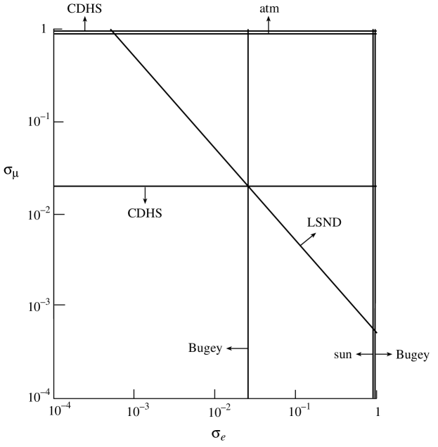
Figure 7: Constraints on $\sigma_{\mu}$ and $\sigma_{e}$ defined in Eq. (31) for the 2+2 model when $\delta m^{2}_{sbl}=1.7$ eV². The LSND, Bugey, CDHS, solar and atmospheric constraints are obtained by comparison of the appropriate data with Eqs. (32), (29), (30), (33), and (34), respectively.

In Fig. 7 we have drawn the $\sigma_{e}$–$\sigma_{\mu}$ plot for the 2+2 model, analogous to the $P_{e3}$–$P_{\mu 3}$ plot for the 1+3 model, for $\delta m^{2}_{sbl}=1.7$ eV². The allowed regions with $\sigma_{\mu}$ near unity (implying near–maximal mixing of $\nu_{\mu}$ in the $\nu_{2}$–$\nu_{3}$ pair) and $\sigma_{e}$ small (implying almost no mixing of $\nu_{e}$ into the $\nu_{2}$–$\nu_{3}$ pair) show that the 2+2 model can comfortably accommodate the data.

Since only mass-squared differences are important for oscillations, the inverted 2+2 model, where the solar oscillations are driven by the mass-squared difference of the upper mass pair and the atmospheric oscillations are driven by the mass-squared difference of the lower mass pair, is equally viable.

4.3 New results

Two features of the data are especially noteworthy. The first is the remarkably high degree of isolation of $\nu_{e}$ into one mass pair and $\nu_{\mu}$ into the other mass pair, as inferred from the bounds on the disappearance amplitudes. The second is the near saturation of the vector inequality in Eq. (32) by the LSND appearance amplitude $A^{\mu e}_{sbl}$ for $\delta m^{2}_{sbl}\simeq 0.3$ eV².

Equations (29) and (30) bound the degree to which $\nu_{e}$ and $\nu_{\mu}$ are found in opposite pairs of mass eigenstates. Without loss of generality we assume that $\nu_{e}$ is predominantly associated with $\nu_{0}$ and $\nu_{1}$, and that $\nu_{\mu}$ is predominantly associated with $\nu_{2}$ and $\nu_{3}$. Then from the Bugey and CDHS data we find the constraints

$$\sigma_{e}\simeq\frac{1}{4}\,A^{e\not e}_{sbl}\leq 0.016\,(0.009)\,,$$ (36)

and

$$1-\sigma_{\mu}\simeq\frac{1}{4}\,A^{\mu\not\mu}_{sbl}\leq 0.013\,(0.2)\,,$$ (37)

respectively, for $\delta m^{2}_{sbl}=2$ eV² ($0.3$ eV²). We then deduce

$$A^{e\not e}_{sbl}\leq 0.065\,(0.04)\,,$$ (38)

which can be compared to the LSND data

$$A^{\mu e}_{sbl}\simeq 0.0025\,(0.04)\,,$$ (39)

for these two values of $\delta m^{2}_{sbl}$. The near–saturation of the inequality in Eq. (35) for $\delta m^{2}_{sbl}=0.3$ eV² has very interesting implications. It means that $\hat{v}_{e}$ is nearly parallel or antiparallel to $\hat{v}_{\mu}$, which in turn indicates that

$$|U_{e2}/U_{e3}|\simeq|U_{\mu 2}/U_{\mu 3}|\,.$$ (40)

This is a new result.

Furthermore, the SuperK data suggest that $\nu_{\mu}$ is maximally mixed in the mass pair with mass-squared difference $\delta m^{2}_{atm}$, so for this pair, called $\nu_{2}$ and $\nu_{3}$, that

$$|U_{\mu 2}|\simeq|U_{\mu 3}|\simeq{1\over\sqrt{2}}.$$ (41)

Then Eq. (40) implies

$$|U_{e2}|\simeq|U_{e3}|.$$ (42)

This is also a new result. In summary, if the oscillation parameters are indeed near the limits of the Bugey bound, the four–neutrino mixing matrix in the 2+2 model must satisfy Eq. (40), which implies Eq. (42) if the atmospheric $\nu_{\mu}$ mixing is maximal.

We can derive additional constraints by considering $\sigma_{e}^{\prime}=P_{e0}+P_{e1}$ and $\sigma_{\mu}^{\prime}=P_{\mu 0}+P_{\mu 1}$ rather than $\sigma_{e}$ and $\sigma_{\mu}$. The data requires $\sigma_{e}^{\prime}$ to be large ($\simeq 1$) and $\sigma_{\mu}^{\prime}$ small, and the Schwartz inequality reduces to

$$A^{\mu e}_{sbl}\leq A^{\mu\not\mu}_{sbl}\,,$$ (43)

where the CDHS bound is

$$A^{\mu\not\mu}_{sbl}\leq 0.05\,(0.8)\,,$$ (44)

at $\delta m^{2}_{sbl}=2.0$ eV² ($0.3$ eV²). Because the inequality in Eq. (43) is not saturated by the data for any $\delta m^{2}_{sbl}$, a relation similar to Eq. (40) for $U_{e0}$, $U_{e1}$, $U_{\mu 0}$, and $U_{\mu 1}$ is not required in the 2+2 model. However, the explicit mass matrices we consider do have such additional relations; see Sec. 5.

Finally, we mention a curiosity [49] in the data which occurs for the pair of pairs mass spectrum with the matter–enhanced solar solutions (SAM and LAM). The linear mass splitting at the heavier pair is $m_{3}-m_{2}\sim\delta m_{32}^{2}/2m_{3}$. If this pair is associated with the atmospheric scale, we have $m_{3}-m_{2}\sim 2.5\times 10^{-2}{\rm eV}\,(\delta m^{2}_{atm}/5\times 10^{-3}{\rm eV}^{2})(m_{3}/{\rm eV})^{-1}$. On the other hand, if the lighter mass pair is associated with the matter–enhanced solar scale, and $m_{0}\gg m_{1}$, then the linear mass–splitting of this pair is $m_{0}-m_{1}\sim m_{0}\sim\sqrt{\delta m^{2}_{sun}}=2.5\times 10^{-2}\,{\rm eV}\,(\delta m^{2}_{sun}/10^{-5}{\rm eV}^{2})^{\frac{1}{2}}$. The two linear mass splittings within the pairs are nearly identical. While squared masses enter into the oscillation formulae for relativistic neutrinos, the more fundamental constructs of field theory, such as the Lagrangian and the resulting equations of motion, are linear in fermion masses (and quadratic in boson masses, these powers of mass being related to the dimensionality of the fermion field vs. the boson field). Thus it is a worthy enterprise to attempt to deduce linear neutrino–mass relations whenever possible.

5 Mass matrix ansatzes

5.1 Solar $\nu_{e}\rightarrow\nu_{s}$ oscillations

To describe the above oscillation phenomena in the scenario where the solar neutrino deficit is described by $\nu_{e}\rightarrow\nu_{s}$ oscillations and the atmospheric data by $\nu_{\mu}\rightarrow\nu_{\tau}$, we consider the neutrino mass matrix ansatz

$$M=m\left(\begin{array}[]{cccc}\epsilon_{1}&\epsilon_{2}&0&0\\ \epsilon_{2}&0&0&\epsilon_{3}\\ 0&0&\epsilon_{4}&1\\ 0&\epsilon_{3}&1&\epsilon_{4}\end{array}\right)\;,$$ (45)

presented in the ($\nu_{s},\nu_{e},\nu_{\mu},\nu_{\tau}$) basis (i.e. the basis where the charged lepton mass matrix is diagonal). By considering the field redefinitions $\Psi\rightarrow-\Psi$ and $\Psi\rightarrow\gamma_{5}\Psi$ one realizes that $m$, and at least one of $\epsilon_{1}$ and $\epsilon_{4}$, and at least one of $\epsilon_{2}$ and $\epsilon_{3}$, may be taken as positive; we will take $m$ and all four $\epsilon_{j}$ to be positive for simplicity. The mass matrix $M$ contains five parameters ($m$, $\epsilon_{1}$, $\epsilon_{2}$, $\epsilon_{3}$, $\epsilon_{4}$), just enough to incorporate the required three mass-squared differences and the oscillation amplitudes for solar and LSND neutrinos. The large amplitude for atmospheric oscillations does not require a sixth parameter in our model because the structure of the mass matrix naturally gives maximal mixing of $\nu_{\mu}$ with $\nu_{\tau}$ (or with $\nu_{s}$ if $\nu_{\tau}$ and $\nu_{s}$ are interchanged).

For simplicity, we have taken the mass matrix to be real and symmetric. The choice of a symmetric neutrino mass matrix is well–motivated in the context of oscillations, for what is measured in neutrino oscillations are the differences of squared masses, which are eigenvalues of the hermitian matrix $MM^{{\dagger}}$, which is itself symmetric when CP conservation is assumed. $M$ is diagonalized by an orthogonal matrix $U$ (real) and there is no CP violation. The $\epsilon_{j}$ are assumed to be small compared to unity, but not all necessarily of the same order of magnitude. The zero terms in the mass matrix could be taken as nonzero without changing the phenomenology discussed here as long as they are small compared to the terms shown. Also, the $M_{\nu_{\mu}\nu_{\mu}}$ term could be chosen different from $\epsilon_{4}$ while still giving maximal mixing of $\nu_{\mu}$ and $\nu_{\tau}$ since maximal mixing results from the large value of the $M_{\nu_{\mu}\nu_{\tau}}$ matrix element relative to the diagonal $M_{\nu_{\mu}\nu_{\mu}}$ and $M_{\nu_{\tau}\nu_{\tau}}$ elements, without any need for fine tuning of the difference $|M_{\nu_{\mu}\nu_{\mu}}-M_{\nu_{\tau}\nu_{\tau}}|$. Here we choose to take the minimal form for $M$ needed to describe the data and then derive the associated consequences.

To a good approximation, the two large eigenvalues of the mass matrix in Eq. (45) are

$$\textstyle m_{2,3}=\mp m\left(1\mp\epsilon_{4}+{1\over 2}\epsilon_{3}^{2}\right)\;.$$ (46)

The values of the two small eigenvalues depend on the hierarchy of the $\epsilon_{j}$. For the three solar cases we have:

$${\rm SAM}: \epsilon_{2}\ll\epsilon_{1},\epsilon_{4}\ll\epsilon_{3}\ll 1\,\,,$$ (47)

$${\rm LAM}: \epsilon_{1},\epsilon_{2},\epsilon_{4}\ll\epsilon_{3}\ll 1\,\,,$$ (48)

$${\rm VLW}: \epsilon_{1}\ll\epsilon_{2}\ll\epsilon_{4}\ll\epsilon_{3}\ll 1\,.$$ (49)

The two small eigenvalues are then approximately given by

$${\rm SAM}: m_{0}\simeq m\epsilon_{1}\,,\quad m_{1}\simeq m(\epsilon_{3}^{2}\epsilon_{4}-\epsilon_{2}^{2}/\epsilon_{1})\,\,,$$ (50)

$${\rm LAM}: m_{0,1}\simeq{m\over 2}\left[\epsilon_{1}\pm\sqrt{\epsilon_{1}^{2}+4\epsilon_{2}^{2}}\right]\,\,,$$ (51)

$${\rm VLW}: m_{0,1}\simeq m\left[\pm\epsilon_{2}+\epsilon_{3}^{2}\epsilon_{4}/2\right]\,.$$ (52)

These approximate expressions for the eigenvalues have been obtained by multiplying each $\epsilon_{j}$ by powers of a hypothetical parameter $\delta$, where the number of powers of $\delta$ assigned to each $\epsilon_{j}$ depends upon the ordering in Eqs. (47)-(49). For example, in the SAM case $\epsilon_{3}$ are multiplied by $\delta$, $\epsilon_{1}$ and $\epsilon_{4}$ by $\delta^{2}$, and $\epsilon_{2}$ by $\delta^{3}$. Then each eigenvalue is written as an expansion in powers of $\delta$, the coefficients of which may be solved for by requiring that the expression $\Pi_{i}(\lambda-\lambda_{i})$ reproduces the eigenvalue equation for the mass matrix order by order in $\delta$. Once the coefficients are found, $\delta$ is set equal to unity.

The eigenvalues in all cases have the desired hierarchy $m_{1}<m_{0}\ll m_{2},m_{3}$, which gives the mass spectrum of the 2+2 model described in Sec. 4.2 and depicted in Fig. 1. The small relative mass splitting of the heavier masses $m_{2},m_{3}$ is governed entirely by the parameter $\epsilon_{4}$: $\delta m^{2}_{32}\simeq 4m^{2}\epsilon_{4}$. The LSND $\nu_{\mu}\rightarrow\nu_{e}$ oscillations are driven by the scale $\delta m^{2}_{21}\simeq\delta m^{2}_{31}\simeq\delta m^{2}_{20}\simeq\delta m^{2}_{30}\simeq m^{2}$, the atmospheric $\nu_{\mu}$ oscillations are determined by $\delta m^{2}_{32}$, and the solar $\nu_{e}\rightarrow\nu_{s}$ oscillations are determined by $\delta m^{2}_{10}$, the approximate expression for which can be obtained by Eqs. (50)-(52). The charged-current eigenstates are approximately related to the mass eigenstates by

$$\left(\begin{array}[]{c}\nu_{s}\\ \nu_{e}\\ \nu_{\mu}\\ \nu_{\tau}\end{array}\right)=U\left(\begin{array}[]{c}\nu_{0}\\ \nu_{1}\\ \nu_{2}\\ \nu_{3}\end{array}\right)\simeq\left(\begin{array}[]{cccc}\cos\theta&-\sin\theta&\cdots&\cdots\\ \sin\theta&\cos\theta&{1\over\sqrt{2}}\epsilon_{3}&{1\over\sqrt{2}}\epsilon_{3}\\ -\epsilon_{3}\sin\theta&-\epsilon_{3}\cos\theta&{1\over\sqrt{2}}&{1\over\sqrt{2}}\\ \cdots&\cdots&-{1\over\sqrt{2}}&{1\over\sqrt{2}}\end{array}\right)\left(\begin{array}[]{c}\nu_{0}\\ \nu_{1}\\ \nu_{2}\\ \nu_{3}\end{array}\right)\;,$$ (53)

where $\tan 2\theta=2\epsilon_{2}/\epsilon_{1}$. The dots indicate nonzero terms that are much smaller than the terms shown. It is their smallness that suppresses mixing between $\nu_{\tau}$ and $\nu_{s}$. The mixing matrix $U$ depends on just three of the original five parameters; it is independent of $\epsilon_{4}$ and the overall mass–scale parameter $m$. Note that $\nu_{0}$ and $\nu_{1}$ couple predominantly to $\nu_{s}$ and $\nu_{e}$. The nearly–degenerate $\nu_{2}$ and $\nu_{3}$ are seen to consist primarily of nearly equal mixtures of $\nu_{\mu}$ and $\nu_{\tau}$. These results, illustrated in Fig. 2, conform to the qualitative arguments of Sec. 3 based on probability rectangles.

It is noted that this mixing matrix not only satisfies the approximate equalities of Eqs. (40)–(42), but in fact replaces the approximate equalities, derived from parameter–independent arguments, with exact equalities to first order in $\epsilon_{j}$. Inspection of the mixing matrix reveals that our model predicts saturation of Eqs. (35) and (43) to this order, i.e., $A^{e\not e}_{sbl}=A^{\mu\not\mu}_{sbl}=A^{\mu e}_{sbl}$. A small improvement in the measurement of $A^{e\not e}_{sbl}$ or a modest improvement in the measurement of $A^{\mu\not\mu}_{sbl}$ is predicted to show a positive disappearance signal.

5.2 Solar $\nu_{e}\rightarrow\nu_{\tau}$ oscillations

Another scenario, with solar $\nu_{e}\rightarrow\nu_{\tau}$ and atmospheric $\nu_{\mu}\rightarrow\nu_{s}$ oscillations, is readily obtained by interchanging $\nu_{\tau}\rightarrow\nu_{s}$ and $\nu_{s}\rightarrow-\nu_{\tau}$. The mass matrix in the ($\nu_{s}$, $\nu_{e}$, $\nu_{\mu}$, $\nu_{\tau}$) basis is then

$$M=m\left(\begin{array}[]{cccc}\epsilon_{4}&\epsilon_{3}&1&0\\ \epsilon_{3}&0&0&-\epsilon_{2}\\ 1&0&\epsilon_{4}&0\\ 0&-\epsilon_{2}&0&\epsilon_{1}\end{array}\right)\;.$$ (54)

The eigenvalues and parameter hierarchies are still given by Eqs. (46)-(52). The mixing matrix is then given by

$$\left(\begin{array}[]{c}\nu_{s}\\ \nu_{e}\\ \nu_{\mu}\\ \nu_{\tau}\end{array}\right)=U\left(\begin{array}[]{c}\nu_{0}\\ \nu_{1}\\ \nu_{2}\\ \nu_{3}\end{array}\right)\simeq\left(\begin{array}[]{cccc}\cdots&\cdots&-{1\over\sqrt{2}}&{1\over\sqrt{2}}\\ \sin\theta&\cos\theta&{1\over\sqrt{2}}\epsilon_{3}&{1\over\sqrt{2}}\epsilon_{3}\\ -\epsilon_{3}\sin\theta&-\epsilon_{3}\cos\theta&{1\over\sqrt{2}}&{1\over\sqrt{2}}\\ -\cos\theta&\sin\theta&\cdots&\cdots\end{array}\right)\left(\begin{array}[]{c}\nu_{0}\\ \nu_{1}\\ \nu_{2}\\ \nu_{3}\end{array}\right)\;,$$ (55)

where again $\tan 2\theta=2\epsilon_{2}/\epsilon_{1}$.

In the VLW case, the parameter $\epsilon_{1}$ is negligibly small if the solar oscillations are maximal, and can be taken as zero without affecting the phenomenology. If this is done, then reference to the mass matrix shows that both $\nu_{e}$ and $\nu_{\tau}$ derive their masses entirely from flavor non–diagonal couplings, and they are maximally mixed (analogous to the $\nu_{\mu}$–$\nu_{s}$ system). Also, if $\epsilon_{1}$ is taken as zero, then there are only four independent parameters needed in the mass matrix, and just two in the mixing matrix. The derived $\theta$ parameter becomes $\pm\frac{\pi}{4}$, and the mixing matrix becomes very simple:

$$U\simeq\frac{1}{\sqrt{2}}\left(\begin{array}[]{cccc}\cdots&\cdots&-1&1\\ \pm 1&1&\epsilon_{3}&\epsilon_{3}\\ \mp\epsilon_{3}&-\epsilon_{3}&1&1\\ -1&\pm 1&\cdots&\cdots\end{array}\right)$$ (56)

5.3 Solar $\nu_{e}\rightarrow\nu_{s}$ and $\nu_{e}\rightarrow\nu_{\tau}$ oscillations

A more general scenario which is a mixture of the previous two is for solar neutrinos to undergo both $\nu_{e}\rightarrow\nu_{s}$ and $\nu_{e}\rightarrow\nu_{\tau}$ oscillations. This is easily parameterized by replacing the $\nu_{s}$ and $\nu_{\tau}$ states in Eq. (53) with the rotated states $\nu_{s}^{\prime}$ and $\nu_{\tau}^{\prime}$ and defining

$$\left(\begin{array}[]{c}\nu_{s}^{\prime}\\ \nu_{\tau}^{\prime}\end{array}\right)=\left(\begin{array}[]{cc}\cos\alpha&-\sin\alpha\\ \sin\alpha&\cos\alpha\end{array}\right)\left(\begin{array}[]{c}\nu_{s}\\ \nu_{\tau}\end{array}\right)\;.$$ (57)

Then the mass matrix in the ($\nu_{s}$, $\nu_{e}$, $\nu_{\mu}$, $\nu_{\tau}$) basis becomes

$$M=m\left(\begin{array}[]{cccc}\epsilon_{1}\cos^{2}\alpha+\epsilon_{4}\sin^{2}\alpha&\epsilon_{2}\cos\alpha+\epsilon_{3}\sin\alpha&\sin\alpha&(\epsilon_{4}-\epsilon_{1})\sin\alpha\cos\alpha\\ \epsilon_{2}\cos\alpha+\epsilon_{3}\sin\alpha&0&0&\epsilon_{3}\cos\alpha-\epsilon_{2}\sin\alpha\\ \sin\alpha&0&\epsilon_{4}&\cos\alpha\\ (\epsilon_{4}-\epsilon_{1})\sin\alpha\cos\alpha&\epsilon_{3}\cos\alpha-\epsilon_{2}\sin\alpha&\cos\alpha&\epsilon_{4}\cos^{2}\alpha+\epsilon_{1}\sin^{2}\alpha\end{array}\right)\;,$$ (58)

and the matrix which diagonalizes $M$ is

$$\left(\begin{array}[]{c}\nu_{s}\\ \nu_{e}\\ \nu_{\mu}\\ \nu_{\tau}\end{array}\right)=U\left(\begin{array}[]{c}\nu_{0}\\ \nu_{1}\\ \nu_{2}\\ \nu_{3}\end{array}\right)=\left(\begin{array}[]{cccc}\cos\theta\cos\alpha&-\sin\theta\cos\alpha&-{1\over\sqrt{2}}\sin\alpha&{1\over\sqrt{2}}\sin\alpha\\ \sin\theta&\cos\theta&{1\over\sqrt{2}}\epsilon_{3}&{1\over\sqrt{2}}\epsilon_{3}\\ -\epsilon_{3}\sin\theta&-\epsilon_{3}\cos\theta&{1\over\sqrt{2}}&{1\over\sqrt{2}}\\ -\cos\theta\sin\alpha&\sin\theta\sin\alpha&-{1\over\sqrt{2}}\cos\alpha&{1\over\sqrt{2}}\cos\alpha\end{array}\right)\left(\begin{array}[]{c}\nu_{0}\\ \nu_{1}\\ \nu_{2}\\ \nu_{3}\end{array}\right)\;,$$ (59)

where $\tan 2\theta=2\epsilon_{2}/\epsilon_{1}$ as before.

6 Oscillation probabilities

6.1 Expressions for any baseline

For the mixing in Eq. (53) (when the solar oscillations are $\nu_{e}\rightarrow\nu_{s}$), the off-diagonal vacuum oscillation probabilities obtained from Eq. (2), to leading order in $\epsilon_{j}$ for each $\Delta_{ij}$ and ignoring amplitudes smaller than ${\cal O}(\epsilon_{j}^{2})$, are

$$P(\nu_{e}\leftrightarrow\nu_{\mu}) \simeq \epsilon_{3}^{2}\left[2\cos^{2}\theta(\sin^{2}\Delta_{21}+\sin^{2}\Delta_{31})-\sin^{2}\Delta_{32}\right.$$ (60)

$${}+\left.2\sin^{2}\theta(\sin^{2}\Delta_{20}+\sin^{2}\Delta_{30})-\sin^{2}2\theta\sin^{2}\Delta_{01}\right]\;,$$

$$P(\nu_{e}\leftrightarrow\nu_{\tau}) \simeq \epsilon_{3}^{2}\sin^{2}\Delta_{32}\;,$$ (61)

$$P(\nu_{e}\leftrightarrow\nu_{s}) \simeq \sin^{2}2\theta\sin^{2}\Delta_{01}\;,$$ (62)

$$P(\nu_{\mu}\leftrightarrow\nu_{\tau}) \simeq \sin^{2}\Delta_{32}\;,$$ (63)

$$P(\nu_{\mu}\leftrightarrow\nu_{s}) \simeq \sin^{2}2\theta\epsilon_{3}^{2}\sin^{2}\Delta_{01}\;,$$ (64)

where $\Delta_{01}\ll\Delta_{32}\ll\Delta_{20}\simeq\Delta_{30}\simeq\Delta_{21}\simeq\Delta_{31}$ due to the neutrino mass spectrum. In our model, only the $\nu_{\tau}$–$\nu_{s}$ oscillation is suppressed beyond ${\cal O}(\epsilon_{j}^{2})$.

6.2 Short baseline

For small $L/E$ only the leading oscillations $\Delta_{20}\simeq\Delta_{21}\simeq\Delta_{30}\simeq\Delta_{31}$ contribute, and the only appreciable oscillation probability is

$$P(\nu_{e}\leftrightarrow\nu_{\mu})\simeq 4\epsilon_{3}^{2}\sin^{2}\Delta\;,$$ (65)

where $\Delta\equiv m^{2}L/4E$. From Eq. (65) we can fix two model parameters

$$\delta m^{2}_{sbl}=m^{2}\;,\quad A^{\mu e}_{sbl}=4\epsilon_{3}^{2}\;.$$ (66)

Since the only short–baseline oscillation is $\nu_{e}\leftrightarrow\nu_{\mu}$, these models predict the equality of the $\nu_{e}$ disappearance probability, the $\nu_{\mu}$ disappearance probability, and the LSND $\nu_{\mu}\rightarrow\nu_{e}$ appearance probability in short–baseline experiments.

6.3 Long baseline

For $L/E$ typical to atmospheric or long baseline neutrino experiments, the oscillations in $\Delta$ assume their average values. The $\Delta_{32}$ oscillation is now evident, and the non-negligible oscillation probabilities in vacuum are

$$P(\nu_{\mu}\leftrightarrow\nu_{\tau})\simeq\sin^{2}\Delta_{32}\;,$$ (67)

$$P(\nu_{e}\leftrightarrow\nu_{\mu})\simeq\epsilon_{3}^{2}\left(2-\sin^{2}\Delta_{32}\right)\;,$$ (68)

$$P(\nu_{e}\leftrightarrow\nu_{\tau})\simeq\epsilon_{3}^{2}\sin^{2}\Delta_{32}\;.$$ (69)

From Eq. (67)

$$\delta m^{2}_{atm}=\delta m^{2}_{32}\simeq 4m^{2}\epsilon_{4}\;,\quad A^{\mu\not\mu}_{atm}=1\;,$$ (70)

which determines another parameter of the model. The model automatically gives maximal oscillations for atmospheric $\nu_{\mu}$’s, while oscillations in other channels are suppressed. The $\nu_{\mu}$ maximal mixing is natural in the sense that it results from the large value of the $M_{\nu_{\mu}\nu_{\tau}}$ matrix element relative to the diagonal $M_{\nu_{\mu}\nu_{\mu}}$ and $M_{\nu_{\tau}\nu_{\tau}}$ elements, without any need for fine tuning of the difference $|M_{\nu_{\mu}\nu_{\mu}}-M_{\nu_{\tau}\nu_{\tau}}|$.

6.4 Extraterrestrial baseline

Finally, for very large $L/E\gg(\delta m^{2}_{atm}/{\rm eV}^{2})^{-1}$ km/GeV, $\sin^{2}\Delta_{32}$ averages to ${1\over 2}$ and the appreciable oscillations in vacuum are

$$P(\nu_{e}\leftrightarrow\nu_{s})\simeq \sin^{2}2\theta\sin^{2}\Delta_{01}\,,$$ (71)

$$P(\nu_{\mu}\leftrightarrow\nu_{s})\simeq \epsilon_{3}^{2}\sin^{2}2\theta\sin^{2}\Delta_{01}\;,$$ (72)

$$P(\nu_{e}\leftrightarrow\nu_{\mu})\simeq \epsilon_{3}^{2}\left[{3\over 2}-\sin^{2}2\theta\sin^{2}\Delta_{01}\right]\,,$$ (73)

$$P(\nu_{e}\leftrightarrow\nu_{\tau})\simeq {1\over 2}\epsilon_{3}^{2}\,,$$ (74)

$$P(\nu_{\mu}\leftrightarrow\nu_{\tau})\simeq {1\over 2}\;.$$ (75)

The solar data can then be explained if the parameters in vacuum satisfy

$${\rm SAM}: \delta m^{2}_{sun}=\delta m^{2}_{01}\simeq m^{2}\epsilon_{1}^{2}\;,\quad A^{e\not e}_{sun}={4\epsilon_{2}^{2}\over 4\epsilon_{2}^{2}+\epsilon_{1}^{2}}\simeq{4\epsilon_{2}^{2}\over\epsilon_{1}^{2}}\;,$$ (76)

$${\rm LAM}: \delta m^{2}_{sun}=\delta m^{2}_{01}\simeq m^{2}\epsilon_{1}\sqrt{\epsilon_{1}^{2}+4\epsilon_{2}^{2}}\;,\quad A^{e\not e}_{sun}={4\epsilon_{2}^{2}\over 4\epsilon_{2}^{2}+\epsilon_{1}^{2}}\;,$$ (77)

$${\rm VLW}: \delta m^{2}_{sun}=\delta m^{2}_{01}\simeq 2m^{2}\epsilon_{2}\epsilon_{3}^{2}\epsilon_{4}\;,\quad A^{e\not e}_{sun}={4\epsilon_{2}^{2}\over 4\epsilon_{2}^{2}+\epsilon_{1}^{2}}\simeq 1\;,$$ (78)

in the three cases.

6.5 Determination of the parameters

In any of these scenarios in Sec. 5.1-5.3, the parameters $m$, $\epsilon_{2}$, $\epsilon_{3}$, $\epsilon_{4}$, and $\epsilon_{1}$ are obtained from the data in exactly the same way, i.e., via Eqs. (66), (70), and (76)-(78). This is a consequence of the $\nu_{s}$–$\nu_{\tau}$ ambiguity. In all cases, the parameters $m$, $\epsilon_{3}$, and $\epsilon_{4}$ are related to the observables by

$$m^{2}=\delta m^{2}_{sbl}\,,\quad\epsilon_{3}^{2}={A^{\mu e}_{sbl}\over 4}\,,\quad\epsilon_{4}={\delta m^{2}_{atm}\over 4\delta m^{2}_{sbl}}\;.$$ (79)

In the solar sector we have

$${\rm SAM}: \epsilon_{1}^{2}={\delta m^{2}_{sun}\over\delta m^{2}_{sbl}}\,,\quad\epsilon_{2}^{2}={A^{e\not e}_{sun}\delta m^{2}_{sun}\over 4\delta m^{2}_{sbl}}\,\,,$$ (80)

$${\rm LAM}: \epsilon_{1}^{2}={\delta m^{2}_{sun}\sqrt{1-A^{e\not e}_{sun}}\over\delta m^{2}_{sbl}}\,,\quad\epsilon_{2}^{2}={\delta m^{2}_{sun}A^{e\not e}_{sun}\over 4\delta m^{2}_{sbl}\sqrt{1-A^{e\not e}_{sun}}}\,\,,$$ (81)

$${\rm VLW}: \epsilon_{1}\simeq 0\,,\quad\epsilon_{2}={8\delta m^{2}_{sun}\over A^{\mu e}_{sbl}\delta m^{2}_{atm}}\,\,.$$ (82)

For the specific values $\delta m^{2}_{sbl}=2{\rm~{}eV}^{2}$ and $A^{\mu e}_{sbl}=2.5\times 10^{-3}$, $\delta m^{2}_{atm}=5\times 10^{-3}\rm~{}eV^{2}$ and $A^{\mu\not\mu}_{atm}=1$, and $\delta m^{2}_{\rm sol.}=4\times 10^{-6}\rm~{}eV^{2}$ and $A^{e\not e}_{sun}=1\times 10^{-2}$, the model parameters are given in Table 3. If we take instead $\delta m^{2}_{sbl}=0.3{\rm~{}eV}^{2}$ and $A^{\mu e}_{sbl}=4.0\times 10^{-2}$ (which gives the smallest value of $\delta m^{2}_{sbl}$ allowed by the data), we get the model parameters shown in Table 4. In either of these two examples, the $\delta m^{2}$ scale for the atmospheric neutrino oscillation can be adjusted simply by varying $\epsilon_{4}$. Also in either case, the two heaviest masses provide relic neutrino targets for a mechanism that may generate the cosmic ray air showers observed above $\mathrel{\raisebox{-2.58334pt}{$\stackrel{{\scriptstyle\textstyle>}}{{\sim}}$}}10^{20}$ eV [50]. We note that the model parameters in Tables 3 and 4 obey the hierarchies described in Eqs. (47)-(49).

7 Model predictions

7.1 Resolving the $\nu_{\tau}$ vs. $\nu_{s}$ ambiguity

If the solar oscillations are $\nu_{e}\rightarrow\nu_{s}$ as described in Sec. 5.1, then our four-neutrino model predicts that the atmospheric oscillations are $\nu_{\mu}\rightarrow\nu_{\tau}$. On the other hand if the solar oscillations are $\nu_{e}\rightarrow\nu_{\tau}$ as in Sec. 5.2, the atmospheric oscillations are $\nu_{\mu}\rightarrow\nu_{s}$. Several possibilities have been discussed to resolve the ambiguous assignment of $\nu_{\tau}$ and $\nu_{s}$ as the oscillation partners of the $\nu_{e}$’s in the sun and the $\nu_{\mu}$’s in the atmosphere. The Solar Neutrino Observatory (SNO) [51], which can measure both charge-current (CC) and neutral-current (NC) interactions, will be able to test whether the solar $\nu_{e}$’s oscillate to sterile or active neutrinos: in the sterile case the CC/NC ratio in SNO will be unity and both CC and NC rates will be suppressed from the SSM predictions, while in the active case only the CC rate is suppressed. Of course if the CC measurement is consistent with the NC, one needs additional evidence to rule out the possibility that the SSM is in error. For instance, SuperKamiokande and SNO can also accurately measure the shape of the ⁸B neutrino spectrum, which would be distorted by oscillations. Also, a measurement of lower energy neutrinos, such as by the BOREXINO experiment [52], could also be used to detect deviations from the SSM spectrum.

Turning to the atmospheric data, the possibilities to resolve the ambiguity center around the earth–matter effects which are possible in the $\nu_{\mu}$-$\nu_{s}$ oscillation channel but not in the $\nu_{\mu}$-$\nu_{\tau}$ channel; there is a relative phase difference between $\nu_{\mu}$ and $\nu_{s}$ due to neutral current forward scattering, but there is no phase difference between $\nu_{\mu}$ and $\nu_{\tau}$. The analytical analysis of matter–effects involving active and sterile neutrinos can be somewhat complicated [20], but the Schrödinger–like evolution equations can always be solved numerically [53]. Other tests have been proposed recently to resolve the $\nu_{\tau}$–$\nu_{s}$ ambiguity. One test is to measure the asymmetry between downward-going and upward-coming events, for electrons and muons separately [54]. Various oscillation scenarios give rise to dramatically differing trajectories of the asymmetries versus energy for muons and electrons. The preliminary data from SuperK for the individual muon and electron asymmetries suggests again that the atmospheric anomaly is primarily due to $\nu_{\mu}$ oscillating into either $\nu_{\tau}$ or $\nu_{s}$, but not $\nu_{e}$. By eventually measuring an up-down asymmetry for neutral current (NC) events (e.g. $\nu N\rightarrow\nu N\pi^{0}$), the ambiguity can be resolved: for the $\nu_{\tau}$ case there is no NC asymmetry, whereas for the $\nu_{s}$ case there is a large NC asymmetry, as shown in Ref. [55]. The ratio of the rates of NC events relative to the charged current (CC) events can be also used to the same end [56], as can multi-ring events [57]. Searches for muon-less events which come from $\nu_{\tau}$, in association with a $\nu_{\mu}$ disappearance measurement, can also in principle distinguish between $\nu_{\tau}$ and $\nu_{s}$ [58].

7.2 New oscillation signals

Assuming that the solar oscillations are $\nu_{e}\rightarrow\nu_{s}$, we can determine the new oscillation signals predicted by the model. Given the order of magnitude of the $\delta m^{2}_{ij}$ and $U_{\alpha j}$, observable new phenomenology occurs for $L/E\gg 1$ km/GeV in the oscillation channels

$$P(\nu_{e}\leftrightarrow\nu_{\mu}) \simeq {1\over 4}A^{\mu e}_{sbl}(2-\sin^{2}\Delta_{atm})\;,$$ (83)

$$P(\nu_{e}\leftrightarrow\nu_{\tau}) \simeq {1\over 4}A^{\mu e}_{sbl}\sin^{2}\Delta_{atm}\;,$$ (84)

where $A^{\mu e}_{sbl}\sim{\cal O}(1\%)$ is the oscillation amplitude which describes the LSND results and $\Delta_{atm}=1.27\delta m^{2}_{atm}L/E\sim(\delta m^{2}_{atm}/5\times 10^{-3}{\rm~{}eV}^{2})(L/157{\rm km})({\rm GeV}/E)$ is the oscillation argument which describes the atmospheric neutrino data. We emphasize the new predictions in the $\nu_{e}\leftrightarrow\nu_{\mu}$ and $\nu_{e}\leftrightarrow\nu_{\tau}$ channels: long baseline oscillations with common oscillation length determined by the atmospheric $\Delta_{atm}$ and common amplitude given by ${1\over 4}$ times the LSND amplitude $A^{\mu e}_{sbl}$. These oscillations are in addition to the $\nu_{\mu}\leftrightarrow\nu_{e}$ oscillations due to $\Delta_{sbl}$ in Eq. (65), which average to the value of ${1\over 2}A^{\mu e}_{sbl}$ in a long baseline experiment. The amplitudes and lengths of these new oscillations complement the set in Table 2, which are inevitable, given the present data, and are therefore required in any model.

How can the oscillation probabilities in Eqs. (83) and (84) be tested? A list of experiments currently underway or being planned to test neutrino oscillation hypotheses is given in Table 5 [59]. In each case the oscillation channel and the parameters which are expected to be tested are shown.

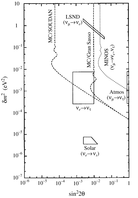
Figure 8: Predicted region in the effective $\delta m^{2}$-$\sin^{2}2\theta$ parameter space for $\nu_{e}\rightarrow\nu_{\tau}$ oscillations in the four-neutrino model (solid rectangle), which is determined by ${1\over 4}$ of the LSND $\nu_{\mu}\rightarrow\nu_{e}$ oscillation amplitude and the atmospheric neutrino $\nu_{\mu}\rightarrow\nu_{\tau}$ oscillation $\delta m^{2}$ scale. The dotted curves show the potential limits on $\nu_{\mu}\rightarrow\nu_{e},\nu_{\tau}$ oscillations from the MINOS experiment [60] and the dashed curves show the potential limits on $\nu_{e},\nu_{\mu}\rightarrow\nu_{\tau}$ oscillations that can be set by neutrino beams from an intense muon source at Fermilab [61] to detectors at the SOUDAN and GRAN SASSO sites for muons with energy of 20 GeV. Also shown are the parameters for the solar $\nu_{e}\rightarrow\nu_{s}$ small-angle MSW oscillation.

The MINOS experiment [60] can detect $\nu_{\mu}\rightarrow\nu_{e}$ or $\nu_{\mu}\rightarrow\nu_{\tau}$ oscillations and is sensitive down to $\delta m^{2}\simeq 10^{-3}$ eV² and a mixing amplitude of $10^{-2}$, which partially overlaps the region of interest; see Fig. 8. If the MINOS experiment can increase its sensitivity, it will provide an even better test of this new phenomenology.

Long–baseline experiments with an intense $\nu_{e}$ or $\bar{\nu}_{e}$ neutrino beam and which can detect $\tau$’s can see the $\nu_{e}\rightarrow\nu_{\tau}$ oscillations in Eq. (84) and provide a definitive test of the new phenomenology predicted by the model. High intensity muon sources [61] can provide simultaneous high intensity $\nu_{\mu}$ and $\bar{\nu}_{e}$ (or $\bar{\nu}_{\mu}$ and $\nu_{e}$ for antimuons) beams with well–determined fluxes, which could then be aimed at a neutrino detector at a distant site. It is expected that $\tau$’s will be detected through their $\mu$ decay mode and that a charge determination can be made, so that one can tell if the $\tau$ originated from $\nu_{\mu}\rightarrow\nu_{\tau}$ or $\bar{\nu}_{e}\rightarrow\bar{\nu}_{\tau}$ oscillations. Current proposals [61] consider SOUDAN ($L=$ 732 km) or GRAN SASSO ($L=$ 9900 km) as the far site from an intense muon source at Fermilab (MC). These experiments could also observe $\nu_{e}\rightarrow\nu_{\mu}$ oscillations via detection of “wrong–sign” muons, i.e., those with sign opposite to that expected from the $\nu_{\mu}$ or $\bar{\nu}_{\mu}$ source. The neutrino energies are in the 10–50 GeV range. Assuming that low backgrounds can be achieved, the sensitivity to $\delta m^{2}$ is roughly proportional to the inverse square root of the detector size (given the same neutrino energy spectrum at the source); the $\delta m^{2}$ sensitivity does not depend on detector distance $L$ because although the flux in the detector falls off with $L^{2}$, the oscillation argument grows with $L^{2}$ for small $\delta m^{2}L/E$. For 20 GeV muons at Fermilab and a 10 kT detector at either SOUDAN or GRAN SASSO, the single–event $\delta m^{2}$ sensitivity for $\nu_{e}\rightarrow\nu_{\tau}$ oscillations is about $8\times 10^{-5}$ eV² for maximal mixing [61]. For large $\delta m^{2}$, the oscillation amplitude single–event sensitivity is roughly inversely proportional to the neutrino flux at the detector divided by the detector size; about $6\times 10^{-5}$ for SOUDAN and $10^{-2}$ for GRAN SASSO [61]. In general, the closer detector has comparable $\delta m^{2}$ sensitivity but better $A$ sensitivity.

The model predicts $\nu_{e}\rightarrow\nu_{\tau}$ oscillations with amplitude $\frac{1}{4}A_{sbl}$ (which ranges from 0.0006 to 0.01) and mass–squared difference of $\delta m^{2}_{atm}$ (which ranges from $3\times 10^{-4}$ to $7\times 10^{-3}$ eV²). The region of possible $\nu_{e}\rightarrow\nu_{\tau}$ oscillations in our model and the regions which can be tested at the SOUDAN and GRAN SASSO sites with a neutrino beam from a high-intensity muon source at Fermilab are shown schematically in Fig. 8, along with the favored parameters for the LSND, atmospheric neutrino, and solar neutrino oscillations. Such experiments would be sensitive to some of the $\nu_{e}\rightarrow\nu_{\tau}$ region, though they may not cover the low–mass, small–amplitude part. These searches would also be able to test the $\nu_{e}\rightarrow\nu_{\mu}$ oscillations in Eq. (83) and the atmospheric $\nu_{\mu}\rightarrow\nu_{\tau}$ oscillations. Additionally, long baseline experiments to the AMANDA detector [62] from Fermilab ($L\simeq$ 11700 km) or KEK ($L\simeq$ 11300 km) may be useful in probing oscillations with small $\delta m^{2}$.

If the solar oscillations are $\nu_{e}\rightarrow\nu_{\tau}$, then the oscillations of atmospheric neutrinos are $\nu_{\mu}\rightarrow\nu_{s}$ and the new oscillations in Eq. (84) are instead $\nu_{e}\rightarrow\nu_{s}$. Neither of these signals would be detectable in long–baseline experiments since the signal is $\nu_{e}$ or $\nu_{\mu}$ disappearance at the few percent level or less. The only measurable signal of the model in this case is the $\nu_{e}\rightarrow\nu_{\mu}$ oscillations in Eq. (83).

If the solar neutrinos oscillate into both $\nu_{s}$ and $\nu_{\tau}$ as given by the mixing in Eq. (59), any vacuum oscillation in Secs. 6.1-6.4 which has $\nu_{s}$ as the final state is replaced by oscillations to $\nu_{s}$ with relative probability $\cos^{2}\alpha$ and to $\nu_{\tau}$ with relative probability $\sin^{2}\alpha$. Conversely, any oscillation which has $\nu_{\tau}$ as the final state is replaced by oscillations to $\nu_{s}$ with relative probability $\sin^{2}\alpha$ and to $\nu_{\tau}$ with relative probability $\cos^{2}\alpha$. In particular, a solar $\nu_{e}$ oscillates into a mixture of $\nu_{s}$ and $\nu_{\tau}$ with relative probability $\cos^{2}\alpha$ and $\sin^{2}\alpha$, respectively, in a vacuum, and an atmospheric $\nu_{\mu}$ oscillates into a mixture of $\nu_{s}$ and $\nu_{\tau}$ with relative probability $\sin^{2}\alpha$ and $\cos^{2}\alpha$, respectively, in a vacuum. The new oscillation signal in Eq. (84) for long baseline experiments is replaced by

$$P(\nu_{e}\leftrightarrow\nu_{\tau})\simeq {1\over 4}A^{\mu e}_{sbl}\cos^{2}\alpha\sin^{2}\Delta_{atm}\;,$$ (85)

$$P(\nu_{e}\leftrightarrow\nu_{s})\simeq {1\over 4}A^{\mu e}_{sbl}\sin^{2}\alpha\sin^{2}\Delta_{atm}\;.$$ (86)

Also, there are new oscillations between $\nu_{s}$ and $\nu_{\tau}$, with the general probability for any baseline given by

$$P(\nu_{s}\rightarrow\nu_{\tau})= \sin^{2}\alpha\cos^{2}\alpha\left[2\cos^{2}\theta(\sin^{2}\Delta_{20}+\sin^{2}\Delta_{30})\right.$$ (87)

$$\left.+2\sin^{2}\theta(\sin^{2}\Delta_{21}+\sin^{2}\Delta_{31})-\sin^{2}\Delta_{32}-\sin^{2}2\theta\sin^{2}\Delta_{01}\right]\;.$$

7.3 Neutrinoless double–$\beta$ decay

Since the $M_{\nu_{e}\nu_{e}}$ mass matrix element is zero in Eq. (45), there is no neutrinoless double-$\beta$ decay at tree level in our model. The present limit on $M_{\nu_{e}\nu_{e}}$ from this process is $\sim$0.5 eV [63]. New experiments are under development which may measure $M_{\nu_{e}\nu_{e}}$ down as low as 0.01 eV[63]. If a nonzero $M_{\nu_{e}\nu_{e}}$ is found at these levels, it would be incompatible with the solar solutions in our models.

7.4 Tritium decay

If $\nu_{e}$ is primarily associated with the lighter pair in the 2+2 model, and $m_{1}<m_{0}\ll m_{2},m_{3}$, then there will be no measurable effect in the endpoint of the tritium decay spectrum. Since only mass-squared differences are important for oscillations, the inverted 2+2 model, where $m_{2},m_{3}\ll m_{1}<m_{0}$, is equally viable, although it is not derivable from the mass matrix in Sec. 5. Then the $\nu_{e}$ will have an effective mass of $0.55-1.4$ eV, which is just below the current limit [64].

7.5 Hot dark matter

For $m\simeq$ 1.4 eV, approximately the largest value allowed by the LSND data, $\sum m_{\nu}\simeq 3$ eV, which according to recent work on early universe formation of the largest structures provides an ideal hot dark matter component [65]. For $m\simeq$ 0.55 eV, the contribution to hot dark matter is much smaller. The contribution of the neutrinos to the mass density of the universe is given by $\Omega_{\nu}=\sum m_{\nu}/(h^{2}93$ eV), where $h$ is the Hubble expansion parameter in units of 100 km/s/Mpc [66]; with $h=0.65$ our model implies $\Omega_{\nu}\simeq 0.05$. An interesting test of neutrino masses is the power spectrum of early galaxy sizes, to be provided by the Sloan Digital Sky Survey (SDSS) [67]. For two nearly degenerate massive neutrino species, sensitivity down to about 0.2 to 0.9 eV (depending on $\Omega$ and $h$) is expected, providing coverage of all or part of the LSND allowed range ($m=$0.55 to 1.4 eV in our model). Also, the future MAP [68] and PLANCK [69] satellite missions, which will measure the cosmic microwave background radiation, should be sensitive to neutrino densities to high precision [70], and in particular to the $\nu_{\mu}\rightarrow\nu_{s}$ atmospheric or the $\nu_{e}\rightarrow\nu_{s}$ large-angle MSW neutrino mixing solutions [71].

7.6 Resonant enhancement in matter

The curves in Fig. 8 (in the scenario where the solar oscillations are $\nu_{e}\rightarrow\nu_{s}$) assume vacuum oscillations in the Earth. In general, large corrections to oscillations involving $\nu_{e}$ and $\nu_{s}$ are possible due to matter. The $\nu_{e}$ diagonal element in the effective mass-squared matrix receives an additional term $\sqrt{2}G_{F}N_{e}E$ from its forward elastic CC interaction, and the $\nu_{s}$ diagonal element receives the contribution $G_{F}N_{n}E/\sqrt{2}$ (relative to the active neutrinos) because it does not have NC interactions. Here, $N_{e}$ and $N_{n}$ denote the electron and neutron number density, respectively. In Table 6 we display the resonant energies in the earth for the various vacuum $\delta m^{2}$ values suggested by the available LSND, atmospheric, and solar data. For neutrinos with energies significantly above $E_{res}$, oscillations are suppressed; for neutrinos with energies significantly below $E_{res}$, the matter effect is negligible; at the resonant energy, $A_{{\rm mat}}=1$ and the oscillation length is increased by $1/\sqrt{A_{{\rm vac}}}$.

Some of the resonant energy values in Table 6 are of particular interest. Upcoming neutrinos from the atmosphere or astrophysical sources, with mass at the lower end of the LSND range, can have their oscillations resonantly enhanced by the earth’s mantle and/or core. Atmospheric neutrinos below a few GeV and the SAM and LAM $pp$ neutrinos from the sun also appear to be near resonance in the earth’s matter. Day–night modulation of the solar flux due to earth–matter effects is expected to discriminate between $\nu_{\tau}$ and $\nu_{s}$ solar fluxes [72, 73], while a precise measurement of zenith angle dependence may discriminate between $\nu_{\tau}$ and $\nu_{s}$ atmospheric fluxes [74]. Oscillation wavelengths commensurate with the size of the earth’s mantle and/or core are especially sensitive.

In our model of Sec. 5.1 with $\nu_{\mu}\rightarrow\nu_{\tau}$ atmospheric neutrino oscillations, however, these corrections do not significantly affect the large $m_{2}^{2}$ and $m_{3}^{2}$ mass eigenvalues as long as $E\ll$ 1 TeV, and hence only modify the $\delta m^{2}_{01}$ oscillation argument. We have verified this by explicit diagonalization of the mass matrix when matter effects are included. Hence we conclude that the matter corrections to the mass matrix in Eq. (45) probably have no observable consequences in all terrestrial experiments. For large $L/E$, such as when $E\mathrel{\raisebox{-2.58334pt}{$\stackrel{{\scriptstyle\textstyle<}}{{\sim}}$}}10$ MeV for solar neutrinos, the only significant effect of matter is the usual MSW enhancement of $\nu_{e}\rightarrow\nu_{s}$ that leads to the solar neutrino suppression of the $\nu_{e}$ flux; in all other oscillation channels the matter–enhanced amplitudes are at the $\epsilon_{\alpha\beta}^{2}$ level or smaller. In the models discussed in Secs. 5.2 and 5.3, where there is a $\nu_{\tau}-\nu_{s}$ component to the atmospheric oscillation, matter effects as discussed here may be important in terrestrial experiments [20].

8 Discussion and summary

8.1 Distinguishing the three solar solutions

The VLW solar solution may be discriminated from the two MSW solutions by a careful measurement of the solar neutrino spectrum by SuperK and BOREXINO [75], or by determining the amount of seasonal variation of the ⁷Be and $pep$ neutrinos [76], which can be measured by the BOREXINO experiment. The ⁸B neutrino spectrum as measured in SuperK and SNO will also be useful in discriminating between the SAM and LAM solutions [77]. The HERON and HELLAZ [78] experiments would be able to measure the $pp$ neutrino energy spectrum, which would also be useful in differentiating the three scenarios.

8.2 Possible $\nu_{\tau}$–$\nu_{s}$ mixing

The general case with $\nu_{s}$-$\nu_{\tau}$ mixing is described in Sec. 5.3. The unmixed cases Eqs. (45) and (54) are obtained in the limits $\alpha\rightarrow 0$ and $\alpha\rightarrow\frac{\pi}{2}$, respectively; distinguishing between the unmixed scenarios is discussed in Sec 7.1. How might non-trivial mixing of $\nu_{\tau}$ and $\nu_{s}$ be observed, and how might the mixing angle be deduced? A mixed model would generally have a signature intermediate between the two unmixed signatures [20]; e.g., experiments measuring neutral current events for solar and atmospheric neutrinos would find a result between those expected for $\nu_{\tau}$ and $\nu_{s}$.

8.3 Summary

An analysis of all the available data (short baseline LSND, reactor and accelerator, long baseline atmospheric, and extraterrestrial length solar) in terms of neutrino oscillations leads to the conclusion that three independent oscillation lengths are contributing. This then further requires mixing of at least four light–mass neutrinos. For a four light–mass neutrino universe, we draw the following model–independent conclusions:
(i) the 1+3 (or 3+1) mass spectrum with a separated mass is disfavored when all the data (LSND, reactor, accelerator, solar, and atmospheric) are considered, leaving a spectrum with two nearly–degenerate pairs as preferred;
(ii) the neutrino mixing matrix elements satisfy $|U_{e2}/U_{e3}|\simeq|U_{\mu 2}/U_{\mu 3}|$ if $\delta m^{2}_{sbl}\simeq 0.3$ eV², i.e., the parameters lie near the Bugey $\nu_{e}$ disappearance limit;
(iii) the relation $|U_{\mu 2}|\simeq|U_{\mu 3}|$ is inferred from the near–maximal mixing of atmospheric $\nu_{\mu}$’s measured by SuperK, which together with (ii) implies $|U_{e2}|\simeq|U_{e3}|$.

Based upon the apparent need for more than three light neutrinos, we have presented four-neutrino models with three active neutrinos and one sterile neutrino. The models naturally have maximal $\nu_{\mu}\rightarrow\nu_{\tau}$ (or $\nu_{\mu}\rightarrow\nu_{s}$) oscillations of atmospheric neutrinos and can also explain the solar neutrino and LSND results. The solar solutions can be $\nu_{e}\rightarrow\nu_{s}$ or $\nu_{e}\rightarrow\nu_{\tau}$, and can be small-angle matter-enhanced, large-angle matter-enhanced, or vacuum long–wavelength oscillations; the increased statistics on the electron energy distribution and day/night differences of the SuperK data [79] may further clarify the allowed regions for the solar solutions. The models predict $\nu_{e}\leftrightarrow\nu_{\tau}$ (or $\nu_{e}\rightarrow\nu_{s}$) and $\nu_{e}\leftrightarrow\nu_{\mu}$ oscillations in long–baseline experiments with $L/E\gg 1$ km/GeV with amplitudes that are determined by the LSND oscillation amplitude and $\delta m^{2}$ scale determined by the oscillation scale of atmospheric neutrinos. For the $\nu_{e}\rightarrow\nu_{\tau}$ case, these oscillations might be seen by experiments based on neutrino beams from an intense muon source at Fermilab with a detector at the SOUDAN or GRAN SASSO sites. The $\nu_{\mu}\rightarrow\nu_{e}$ oscillations might be seen by the MINOS experiment or at KEK with detectors at Kamiokande and SuperKamiokande. The models also predict the equality of the $\nu_{e}$ disappearance probability, the $\nu_{\mu}$ disappearance probability, and the LSND $\nu_{\mu}\rightarrow\nu_{e}$ appearance probability in short–baseline experiments.

9 Acknowledgements

We thank D. Caldwell, R. Foot, P. Krastev, J.G. Learned, S. Petcov, G. Raffelt, J. Stone, and R. Volkas for comments and discussions. This work was supported in part by the U.S. Department of Energy, Division of High Energy Physics, under Grants No. DE-FG02-94ER40817, No. DE-FG05-85ER40226, and No. DE-FG02-95ER40896, and in part by the University of Wisconsin Research Committee with funds granted by the Wisconsin Alumni Research Foundation, the Vanderbilt University Research Council, the University of Hawaii, and the Max Planck Institute for Physics, Munich.

Table 1: Ranges of mass-squared differences and amplitudes that provide oscillation solutions to the solar neutrino data within 95% C.L. in the small–angle MSW, large–angle MSW and vacuum long–wavelenth scenarios when $\nu_{e}\rightarrow\nu_{s}$ or $\nu_{e}\rightarrow\nu_{\tau}$ [39]. The new SuperK data and new solar flux calculations give slightly different oscillation parameters than those quoted here; in particular, the $\delta m^{2}$ values for the VLW solution are higher, of order $4\times 10^{-10}$ eV² [41].

$\nu_{e}\rightarrow\nu_{s}$	SAM	LAM	VLW
$\delta m^{2}$ (eV2)	$3.5\times 10^{-6}$–$7.5\times 10^{-6}$	$\simeq 9\times 10^{-6}$	$\simeq 5\times 10^{-11}$
$A^{es}_{sun}$	$2.5\times 10^{-3}$–$1.6\times 10^{-2}$	$\simeq 0.7$	$\simeq 1$
$\nu_{e}\rightarrow\nu_{\tau}$	SAM	LAM	VLW
$\delta m^{2}$ (eV2)	$4\times 10^{-6}$–$9\times 10^{-6}$	$8\times 10^{-6}$–$3\times 10^{-5}$	$5\times 10^{-11}$–$8\times 10^{11}$
$A^{e\tau}_{sun}$	$3.5\times 10^{-3}$–$1.3\times 10^{-2}$	$0.4$–$0.8$	$0.6$–$1.0$

Table 2: Some typical $\delta m^{2}$ and vacuum oscillation amplitudes suggested by experiment, and the corresponding vacuum oscillation lengths $\lambda_{v}=2.5\,(E_{\nu}/{\rm GeV})(\delta m^{2}/{\rm eV}^{2})^{-1}$ km for representative neutrino energies. Here AU is the earth-sun distance and $R_{\oplus}$ is the earth’s radius.

	$\delta m^{2}/{\rm eV}^{2}$	$A$	$\lambda_{v}=4\pi E_{\nu}/\delta m^{2}$, with $E_{\nu}$ as shown:
			5 MeV	100 MeV	2 GeV	10 GeV	30 GeV	100 GeV	1 TeV
LSND	2	0.0025	6 m	125 m	2.5 km	12 km	37 km	125 km	1250km
LSND	0.3	0.04	42 m	840 m	17 km	83 km	250 km	830 km	1.2 $R_{\oplus}$
ATM	$5\times 10^{-3}$	0.8–1.0	2.5 km	50 km	$10^{3}$ km	5000km	2.3 $R_{\oplus}$	7.8 $R_{\oplus}$	78 $R_{\oplus}$
SAM	$6\times 10^{-6}$	.0025–.016	2100 km	6.5 $R_{\oplus}$	130 $R_{\oplus}$
LAM	$10^{-5}$	0.4–0.8	1260 km	3.9 $R_{\oplus}$	78 $R_{\oplus}$
VLW	$5\times 10^{-11}$	0.6–1.0	1.7 AU	33 AU	670 AU

Table 3: Typical model parameters for the input data $\delta m^{2}_{sbl}=2$ eV², $A^{\mu e}_{sbl}=2.5\times 10^{-3}$, $\delta m^{2}_{atm}=5\times 10^{-3}$ eV², and $A^{\mu\not\mu}_{atm}=1$.

inputs	SAM	LAM	VLW
$\delta m^{2}_{sun}$ (eV2)	$4\times 10^{-6}$	$9\times 10^{-6}$	$5\times 10^{-11}$
$A^{e\not e}_{sun}$	$1\times 10^{-2}$	$0.72$	$1.0$
outputs	SAM	LAM	VLW
$m$ (eV)	$1.4$	$1.4$	$1.4$
$\epsilon_{3}$	$2.5\times 10^{-2}$	$2.5\times 10^{-2}$	$2.5\times 10^{-2}$
$\epsilon_{4}$	$6.3\times 10^{-4}$	$6.3\times 10^{-4}$	$6.3\times 10^{-4}$
$\epsilon_{2}$	$7.1\times 10^{-5}$	$1.2\times 10^{-3}$	$3.2\times 10^{-5}$
$\epsilon_{1}$	$1.4\times 10^{-3}$	$1.5\times 10^{-3}$	$\simeq 0$

Table 4: Typical model parameters for the input data $\delta m^{2}_{sbl}=0.3$ eV², $A^{\mu e}_{sbl}=4.0\times 10^{-2}$, $\delta m^{2}_{atm}=5\times 10^{-3}$ eV², and $A^{\mu\not\mu}_{atm}=1$.

inputs	SAM	LAM	VLW
$\delta m^{2}_{sun}$ (eV2)	$4\times 10^{-6}$	$9\times 10^{-6}$	$5\times 10^{-11}$
$A^{e\not e}_{sun}$	$1\times 10^{-2}$	$0.72$	$1.0$
outputs	SAM	LAM	VLW
$m$ (eV)	$0.55$	$0.55$	$0.55$
$\epsilon_{3}$	$1.0\times 10^{-1}$	$1.0\times 10^{-1}$	$1.0\times 10^{-1}$
$\epsilon_{4}$	$4.2\times 10^{-3}$	$4.2\times 10^{-3}$	$4.2\times 10^{-3}$
$\epsilon_{2}$	$1.9\times 10^{-4}$	$3.2\times 10^{-3}$	$2.0\times 10^{-6}$
$\epsilon_{1}$	$3.7\times 10^{-3}$	$4.0\times 10^{-3}$	$\simeq 0$

Table 5: Current and planned short and long baseline neutrino oscillation experiments. Stars denote accessible oscillation channels. The $\delta m^{2}$ and $\sin^{2}2\theta$ sensitivies are given.

									Test Model?
Experiment	$\displaystyle\nu_{\mu}\atop{\displaystyle\downarrow\atop\displaystyle\nu_{e}}$	$\displaystyle\nu_{\mu}\atop{\displaystyle\downarrow\atop\displaystyle\nu_{\tau}}$	$\displaystyle\nu_{e}\atop{\displaystyle\downarrow\atop\displaystyle\nu_{\tau}}$	$\displaystyle\nu_{e}\atop{\displaystyle\downarrow\atop\displaystyle\nu_{e}}$	$\displaystyle\delta m^{2}\atop\vskip 12.0pt plus 4.0pt minus 4.0pt\rm(eV^{2})$	$\sin^{2}2\theta$	$\displaystyle\rm Test\atop\displaystyle\rm LSND?$	$\displaystyle\rm Test\atop\displaystyle\rm Atmos?$	$\displaystyle\nu_{\mu}\atop{\displaystyle\downarrow\atop\displaystyle\nu_{e}}$	$\displaystyle\nu_{e}\atop{\displaystyle\downarrow\atop\displaystyle\nu_{\tau}}$
BOONE	$\star$				$10^{-2}$	$6\times 10^{-4}$	$\star$
BOREXINO				$\star$	$10^{-6}$	0.4
CHORUS		$\star$			0.3	$2\times 10^{-4}$
COSMOS		$\star$			0.1	$10^{-5}$
ICARUS, NOE,	$\star$	$\star$			$3\times 10^{-3}$	$4\times 10^{-2}$		p
AQUA-RICH, OPERA
KARMEN	$\star$				$4\times 10^{-2}$	$10^{-3}$	$\star$
KamLAND	$\star$				$2\times 10^{-3}$	0.2
K2K	$\star$				$2\times 10^{-3}$	$5\times 10^{-2}$		p
MC/Gran Sasso	$\star$	$\star$	$\star$		$8\times 10^{-5}$	$10^{-2}$	p	$\star$	p	p
MC/Soudan	$\star$	$\star$	$\star$		$8\times 10^{-5}$	$6\times 10^{-5}$	$\star$	$\star$	$\star$	p
MINOS	$\star$	$\star$			$10^{-3}$	$10^{-2}$	p	p	p
NOMAD		$\star$			0.5	$3\times 10^{-4}$
ORLANDO, ESS	$\star$				$3\times 10^{-3}$	$10^{-4}$	$\star$
Palo Verde				$\star$	$10^{-3}$	0.2
TOSCA		$\star$			0.1	$10^{-5}$

p = partially

Table 6: Resonant energies $E_{res}=6.6\,\sqrt{1-A}\,(\delta m^{2}/{\rm eV}^{2})(N_{e}/N_{A}\,{\rm cm}^{-3})^{-1}$ TeV in the earth’s core and mantle for $\nu_{e}$–$\nu_{\mu/\tau}$ oscillations, for some typical vacuum values for the $\delta m^{2}$’s and amplitudes suggested by the data. Here $A$ is the oscillation amplitude and $N_{A}$ is Avagadro’s number. We have taken the core electron density to be 4.5 to 6.0 $N_{A}/{\rm cm}^{3}$, and the mantle density to be 1.6 to 2.6 $N_{A}/{\rm cm}^{3}$. Resonant energies for $\nu_{e}$–$\nu_{s}$ oscillations are $2N_{e}/(2N_{e}-N_{n})$ times larger than for $\nu_{e}$–$\nu_{\mu/\tau}$ oscillations, resonant energies for $\nu_{\mu/\tau}$–$\nu_{s}$ oscillations are $2N_{e}/N_{n}$ times larger, but resonance occurs for ${\bar{\nu}}$ rather than $\nu$ since the phase difference due to matter has the opposite sign.

$A$		$\delta m^{2}/{\rm eV}^{2}$	$E_{res}=\delta m^{2}\sqrt{1-A}/(2\sqrt{2}G_{F}N_{e})$
			core	mantle
$\ll 1$	LSND	2	2.2–2.9 TeV	5.1–8.2 TeV
$\ll 1$	LSND	0.3	330-440 GeV	0.8-1.2 TeV
0.8	ATM	$5\times 10^{-3}$	2.4–3.3 GeV	5.6–9.2 GeV
$\ll 1$	SAM	$6\times 10^{-6}$	6.5–8.8 MeV	15–25 MeV
0.6	LAM	$10^{-5}$	6.9–9.2 MeV	16–26 MeV
0.8	VLW	$5\times 10^{-10}$	25–33 eV	55–90 eV

References

- [1] J.N. Bahcall and M.H. Pinsonneault, Rev. Mod. Phys. 67, 781 (1995); J.N. Bahcall, S. Basu, and M.H. Pinsonneault, astro-ph/9805135; the new solar flux calculation in the second reference has not yet been implemented in the solar neutrino analyses.
- [2] B.T. Cleveland et al., Nucl. Phys. B (Proc. Suppl.) 38, 47 (1995); Kamiokande collaboration, Y. Fukuda et al., Phys. Rev. Lett, 77, 1683 (1996); GALLEX Collaboration, W. Hampel et al., Phys. Lett. B388, 384 (1996); SAGE collaboration, J.N. Abdurashitov et al., Phys. Rev. Lett. 77, 4708 (1996).
- [3] Kamiokande collaboration, K.S. Hirata et al., Phys. Lett. B280, 146 (1992); Y. Fukuda et al., Phys. Lett. B335, 237 (1994); IMB collaboration, R. Becker-Szendy et al., Nucl. Phys. Proc. Suppl. 38B, 331 (1995); Soudan-2 collaboration, W.W.M. Allison et al., Phys. Lett. B391, 491 (1997).
- [4] The Super–Kamiokande Collaboration, talk by E. Kearns in Ref. [8] and hep–ex/9803007; Y. Fukuda et al., hep–ex/9803006 and Phys. Lett. B, to appear.
- [5] The Super–Kamiokande Collaboration, Y. Fukuda et al., hep–ex/9805006.
- [6] J.G. Learned, S. Pakvasa, and T.J. Weiler, Phys. Lett. B207, 79 (1988); V. Barger and K. Whisnant, Phys. Lett. B209, 365 (1988); K. Hidaka, M. Honda, and S. Midorikawa, Phys. Rev. Lett. 61, 1537 (1988).
- [7] Liquid Scintillator Neutrino Detector (LSND) collaboration, C. Athanassopoulos et al., Phys. Rev. Lett. 75, 2650 (1995); ibid. 77, 3082 (1996); nucl-ex/9706006.
-
[8]
For a recent review, see talks at the ITP Conference on Solar Neutrinos:
News About SNUS, Santa Barbara, December 1997 at
http://doug-pc.itp.ucsb.edu/online/snu/schedule.html - [9] C.Y. Cardall and G.M. Fuller, Nucl. Phys. Proc. Suppl. 51B, 259 (1996); G.L. Fogli, E. Lisi, D. Montanino, and G. Scioscia, Phys. Rev. D56, 4365 (1997).
- [10] A. Acker, J.G. Learned, S. Pakvasa and T.J. Weiler, Phys. Lett. B298, 149 (1992); A. Acker and S. Pakvasa, Phys. Lett. B397, 209 (1997);
- [11] P.I. Krastev and S.T. Petcov, Phys. Lett. B395, 69 (1997).
- [12] L.M. Johnson and D. McKay, hep–ph/9805311.
- [13] V. Barger, P. Langacker, J. Leveille, and S. Pakvasa, Phys. Rev. Lett. 45, 692 (1980); Z.G. Berezhiani and R.N. Mohapatra, Phys. Rev. D52, 6607 (1995); E.J. Chun, A.S. Joshipura and A.Y. Smirnov, Phys. Lett. B357, 608 (1995), and Phys. Rev. D54, 4654 (1996); K. Benakli and A.Y. Smirnov, Phys. Rev. Lett 79, 4314 (1997); J.R. Espinosa, hep–ph/9707541; G. Cleaver, M. Cvetic, J.R. Espinosa, L. Everett, and P. Langacker, Phys. Rev. D57, 2701 (1998); P. Langacker, hep–ph/9805281.
- [14] LEP Electroweak Working Group and SLD Heavy Flavor Group, D. Abbaneo et al., CERN-PPE-96-183, December 1996.
- [15] D.O. Caldwell and R.N. Mohapatra, Phys. Rev. D 48, 3259 (1993); J.T. Peltoniemi and J.W.F. Valle, Nucl. Phys. B 406, 409 (1993); R. Foot and R.R. Volkas, Phys. Rev. D 52, 6595 (1995); Ernest Ma and Probir Roy, Phys. Rev. D 52, R4780 (1995); J.J. Gomez-Cadenas and M.C. Gonzalez-Garcia, Z. Phys. C 71, 443 (1996); N. Okada and O. Yasuda, Int. J. Mod. Phys. A 12, 3669 (1997); S.M. Bilenky, C. Giunti, and W. Grimus, hep–ph/9711416; R.N. Mohapatra, hep–ph/9711444; N. Gaur, A. Ghosal, Ernest Ma, and Probir Roy, hep-ph/9806272; particularly strong enthusiasm for the sterile neutrino is expressed by D.O. Caldwell, hep–ph/9804367.
- [16] R. Barbieri and A. Dolgov, Phys. Lett. B237, 440 (1990); K. Enqvist, K. Kainulainen, and M. Thomson, Nucl. Phys. B373, 498 (1992); X. Shi, D.N. Schramm, and B.D. Fields, Phys. Rev. D 48, 2563 (1993); C.Y. Cardall and G.M. Fuller, Phys. Rev. D 54, 1260 (1996); D.P. Kirilova and M.V. Chizhov, hep–ph/9707282; S.M. Bilenky, C. Giunti, W. Grimus and T. Schwetz, hep–ph/9804421.
- [17] P.J. Kernan and S. Sarkar, Phys. Rev. 54, R3681 (1996); S. Sarkar, Reports on Progress in Physics 59, 1 (1996); K.A. Olive, talk at 5th International Workshop on Topics in Astroparticle and Underground Physics (TAUP 97), Gran Sasso, Italy, 1997; K.A. Olive, proc. of 5th International Conference on Physics Beyond the Standard Model, Balholm, Norway, 1997; C.J. Copi, D.N. Schramm and M.S. Turner, Phys. Rev. Lett. 75, 3981 (1995); K.A. Olive and G. Steigman, Phys. Lett. B354, 357 (1995).
- [18] R. Foot and R.R. Volkas, Phys. Rev. Lett. 75, 4350 (1995); R. Foot, M.J. Thompson, and R.R. Volkas, Phys. Rev. D 53, 5349 (1996); N.F. Bell, R. Foot, and R.R. Volkas, hep–ph/9805259.
- [19] R. Foot and R.R. Volkas, Phys. Rev. D55, 5147 (1997);
- [20] Q.Y. Liu and A. Yu. Smirnov, hep–ph/9712493.
- [21] L. Wolfenstein, Phys. Rev. D 17, 2369 (1978);
- [22] S.P. Mikheyev and A. Smirnov, Yad. Fiz. 42, 1441 (1985); Nuovo Cim. 9C, 17 (1986).
- [23] S.P. Rosen and J.M. Gelb, Phys. Rev. D 34, 969 (1986).
- [24] S.J. Parke, Phys. Rev. Lett. 57, 1275 (1986); S.J. Parke and T.P. Walker, Phys. Rev. Lett. 57, 2322 (1986); W.C. Haxton, Phys. Rev. Lett. 57, 1271 (1986); T.K. Kuo and J. Pantaleone, Rev. Mod. Phys. 61, 937 (1989).
- [25] H. Bethe, Phys. Rev. Lett. 56, 1305 (1986); V. Barger, R.J.N. Phillips, and K. Whisnant, Phys. Rev. D 34, 980 (1986);
- [26] V. Barger, R.J.N. Phillips, and K. Whisnant, Phys. Rev. D 24, 538 (1981).
- [27] S.L. Glashow and L.M. Krauss, Phys. Lett. B190, 199 (1987).
- [28] V. Barger, K. Whisnant, D. Cline, and R.J.N. Phillips, Phys. Lett. B93, 194 (1980).
- [29] L. Borodovsky et al., Phys. Rev. Lett. 68, 274 (1992).
- [30] KARMEN collaboration, B. Bodmann et al., Nucl. Phys. A553, 831c (1993); J. Kleinfeller, Nucl. Phys. B48 (proc. Suppl.) 207 (1996); talk by B. Armbruster at 33rd Rencontres de Moriond: Electroweak Interactions and Unified Theories, Les Arcs, France, March 1998.
- [31] Y.–Z. Qian et al., Phys. Rev. Lett. 71, 1965 (1993).
- [32] Y. Declais et al., Nucl. Phys. B434, 503 (1995).
- [33] F. Dydak et al., Phys. Lett. B134, 281 (1984).
- [34] I.E. Stockdale et al., Phys. Rev. Lett. 52, 1384 (1984).
- [35] G. Barr, T.K. Gaisser, and T. Stanev, Phys. Rev. D 39, 3532 (1989); M. Honda, T. Kajita, K. Kasahara, and S. Midorikawa, Phys. Rev. D52, 4985 (1995); V. Agrawal, T.K. Gaisser, P. Lipari, and T. Stanev, Phys. Rev. D 53, 1314 (1996); T.K. Gaisser et al., Phys. Rev. D 54, 5578 (1996).
- [36] M.C. Gonzalez–Garcia, H. Nunokawa, O. Peres, T. Stanev, and J.W.F. Valle, hep-ph/9801368.
- [37] CHOOZ collaboration, M. Apollonio et al., hep-ex/9711002.
- [38] E. Akhmedov, P. Lipari and M. Lusignoli, Phys. Lett. B300, 128 (1993); P. Lipari and M. Lusignoli, hep–ph/9712278, and hep–ph/9803440; R. Foot, R.R. Volkas and O. Yasuda, hep–ph/9801431.
- [39] N. Hata and P. Langacker, Phys. Rev. D56, 6107 (1997).
- [40] P. Krastev and S.T. Petcov, Phys. Rev. Lett. 72, 1960 (1994); Nucl. Phys. B449, 605 (1995).
- [41] Y. Totsuka, talk at Neutrino-98, Takayama, Japan, June 1998.
- [42] V. Barger, K. Whisnant, S. Pakvasa, and R.J.N. Phillips, Phys. Rev. D 22, 2718 (1981).
- [43] P. Langacker, J.P. Leveille, and J. Sheiman, Phys. Rev. D 27, 1228 (1983).
- [44] V. Barger, N. Deshpande, P.B. Pal, R.J.N. Phillips, and K. Whisnant, Phys. Rev. D 43, 1759 (1991); S. Bludman, D.C. Kennedy, and P. Langacker, Nucl. Phys. B374, 373 (1992).
- [45] C. Yanagisawa, talk given at Pheno 98, Madison, WI, April 1998.
- [46] V. Barger, K. Whisnant, and T.J. Weiler, hep–ph/9712495 and Phys. Lett. B, to appear.
- [47] S.C. Gibbons, R.N. Mohapatra, S. Nandi, and A. Raychaudhuri, hep–ph/9803299.
- [48] S. M. Bilenky, C. Giunti and W. Grimus, Eur. Phys. J. C1, 247 (1998) and hep–ph/9607372.
- [49] This was pointed out to us by G. Raffelt.
- [50] T.J. Weiler, hep–ph/9710431, to appear in Astropart. Phys.
- [51] E. Norman et al., Solar Neutrino Observatory (SNO) collaboration, in proc. of The Fermilab Conference: DPF 92, November 1992, Batavia, IL, ed. by C. H. Albright, P.H. Kasper, R. Raja, and J. Yoh (World Scientific, Singapore, 1993), p. 1450.
- [52] BOREXINO Collaboration, C. Arpesella et al., “INFN Borexino proposal,” Vols. I and II, edited by G. Bellini, R. Raghavan et al. (Univ. of Milan, 1992); J. Benziger, F.P. Calaprice et al., “Proposal for Participation in the Borexino Solar Neutrino Experiment,” (Princeton University, 1996).
- [53] A.B. Balantekin, J.F. Beacom, and J.M. Fetter, hep-ph/9712390.
- [54] J. Flanagan, J. G. Learned and S. Pakvasa, Phys. Rev. D57, R2649(1998); J. Bunn, R. Foot and R.R. Volkas, Phys. Lett. B413,109(1997).
- [55] J. G. Learned, S. Pakvasa and J. Stone, hep–ph/9805343.
- [56] F. Vissani and A. Smirnov, hep–ph/9710565.
- [57] L.J. Hall and H. Murayama, hep–ph/9806218.
- [58] A. Curioni et al., hep–ph/9805249.
- [59] For World Wide Web links to more information on these and other neutrino oscillation experiments, see the Neutrino Oscillation Industry web page at http://www.hep.anl.gov/NDK/Hypertext/nuindustry.html.
- [60] MINOS Collaboration, “Neutrino Oscillation Physics at Fermilab: The NuMI-MINOS Project,” NuMI-L-375, May 1998.
- [61] S. Geer, hep–ph/9712290.
- [62] S. Barwick et al., AMANDA collaboration, in proc. XXVIth International Conference on High Energy Physics, Dallas TX, August 1992, ed. by James R. Sanford (AIP, New York, 1993), p. 1250; F. Halzen, astro–ph/9707289.
- [63] H.V. Klapdor–Kleingrothaus, hep–ph/9802007; J. Phys. G24, 483 (1998).
- [64] A.I. Belesev et al., Phys. Lett. B350, 263 (1995); V.M. Lobashev et al., in Proc. of Neutrino ’98, ed. by K. Enqvist, K. Huitu, and J. Maalampi (World Scientific, Singapore, 1997).
- [65] For a recent discussion see J. Primack, astro–ph/9707285.
- [66] E.W. Kolb and M.S. Turner, The Early Universe (Addison-Wesley, Reading, 1990).
- [67] W. Hu, D.J. Eisenstein, and M. Tegmark, astro–ph/9712057.
- [68] See http://map.gsfc.nasa.gov for information on MAP.
- [69] See http://astro.estec.esa.nl/Planck/ for information on PLANCK.
- [70] C.-P. Ma and E. Bertschinger, Astrophys. J. 455, 7 (1995); S. Dodelson, E. Gates, and A. Stebbins, Astrophys. J. 467, 10 (1996); R.E. Lopez, S. Dodelson, A. Heckler, and M.S. Turner, astro–ph/9803095.
- [71] S. Hannestad and G. Raffelt, astro–ph/9805223.
- [72] M. Maris and S.T. Petcov, hep–ph/9803244; S.T Petcov, hep–ph/9805262.
- [73] E.K. Akhmedov, hep–ph/9805272.
- [74] Q.Y. Liu, S.P. Mikheyev, and A.Y. Smirnov, hep–ph/9803415.
- [75] B. Faid, G.L. Fogli, E. Lisi, and D. Montanino, hep–ph/9805293.
- [76] V. Barger, R.J.N. Phillips, and K. Whisnant, Phys. Rev. Lett. 65, 3084 (1990).
- [77] G.L. Fogli, E. Lisi, and D. Montanino, hep–ph/9803309.
- [78] HELLAZ Collaboration, F. Arzarello et al., CERN-LAA/94-19.
- [79] Y. Suzuki, talk at Neutrino-98, Takayama, Japan, June 1998.