Constraints on pre-big bang models for seeding large-scale
anisotropy by massive Kalb–Ramond axions

M. Gasperini

Dipartimento di Fisica Teorica, Università di Torino, Via P. Giuria 1, 10125 Turin, Italy
and Istituto Nazionale di Fisica Nucleare, Sezione di Torino, Turin, Italy

G. Veneziano

Theory Division, CERN, CH-1211 Geneva 23, Switzerland

Abstract

We discuss the conditions under which pre-big bang models can fit the observed large-scale anisotropy with a primordial spectrum of massive (Kalb–Ramond) axion fluctuations. The primordial spectrum must be sufficiently flat at low frequency and sufficiently steeper at high frequency. For a steep and/or long enough high-frequency branch of the spectrum the bounds imposed by COBE’s normalization allow axion masses of the typical order for a Peccei–Quinn–Weinberg–Wilczek axion. We provide a particular example in which an appropriate axion spectrum is obtained from a class of backgrounds satisfying the low-energy string cosmology equations.

[

Constraints on pre-big bang models for seeding large-scale anisotropy
by massive Kalb–Ramond axions M. Gasperini

Dipartimento di Fisica Teorica, Università di Torino, Via P. Giuria 1, 10125 Turin, Italy
and Istituto Nazionale di Fisica Nucleare, Sezione di Torino, Turin, Italy

G. Veneziano

Theory Division, CERN, CH-1211 Geneva 23, Switzerland

(May 1998)

We discuss the conditions under which pre-big bang models can fit the observed large-scale anisotropy with a primordial spectrum of massive (Kalb–Ramond) axion fluctuations. The primordial spectrum must be sufficiently flat at low frequency and sufficiently steeper at high frequency. For a steep and/or long enough high-frequency branch of the spectrum the bounds imposed by COBE’s normalization allow axion masses of the typical order for a Peccei–Quinn–Weinberg–Wilczek axion. We provide a particular example in which an appropriate axion spectrum is obtained from a class of backgrounds satisfying the low-energy string cosmology equations.

]

I INTRODUCTION

It has recently been shown [2, 3] that a stochastic background of massless axions can induce large-scale anisotropies of the Cosmic Microwave Background (CMB), in agreement with present observations [4, 5], provided it is primordially produced with a sufficiently flat spectrum. It has also been shown that a massive axion background can satisfy the same experimental constraints, with some additional restrictions on the tilt of the spectrum, but only if the axion mass lies inside an appropriate ultra-light mass window [2] having an upper limit of $10^{-17}$ eV.

The cosmic axion background considered in [2, 3] is obtained by amplifying the vacuum fluctuations of the so-called universal axion of string theory [6], i.e. the (four-dimensional) dual of the Kalb–Ramond (KR) antisymmetric tensor field appearing in the low-energy string effective action. The KR axion has interactions of gravitational strength, hence its mass is not significantly constrained by present tests of the equivalence principle for polarized macroscopic bodies [7]. Although (gravitationally) coupled to the QCD topological current, the KR axion is not to be necessarily identified with the “invisible” axion [8] responsible for solving the strong CP problem. Other, more strongly coupled pseudoscalars, can play the traditional axion’s role. In this case, the standard Weinberg–Wilczek formula [9] would give the mass of the appropriate combination of pseudoscalars which is coupled to the topological charge, while the KR axion would mostly lie along the orthogonal combinations, which remain (almost) massless.

In this context it is thus possible that KR axions are neither produced from an initial misalignment of the QCD vacuum angle [10], nor from the decay of axionic cosmic strings [11], so that existing cosmological bounds on the axion mass [12] can be evaded. Also, KR axions are treated in [2, 3] as “seeds”, i.e. as inhomogeneous perturbations of a background that is not axion-dominated, so that the mechanism of anisotropy production is different from previous computations of isocurvature axion perturbations [13]. The seed approximation is not inconsistent either with the presence of mass or with the possible resonant amplification of quantum fluctuations through oscillations in the full axion potential [14].

In spite of all this, it is quite likely that the KR axion will be heavier than $10^{-17}$ eV, in which case, taking the results of [2] at face value, KR axions would be unable to seed the observed CMB anisotropies. The main purpose of this paper is to point out that this conclusion is not inescapable, provided one is willing to add more structure to the primordial axion spectrum through more complicated cosmological backgrounds than the one considered in [2].

It turns out, in particular, that the bounds on the axion mass can be relaxed, provided the axion spectrum, before non-relativistic corrections, grows monotonically with frequency, but with a frequency-dependent slope. At low frequencies the slope must be small enough to reproduce the approximate scale-invariant spectrum found by COBE, while at high frequencies the spectrum has to be steeper. Since position and normalization of the end point of the spectrum are basically fixed in string cosmology, the steeper and/or longer the high-frequency spectrum, the larger the suppression of the amplitude at the low-frequency scales relevant for COBE’s observation. On the other hand, the low-frequency amplitude is proportional to a positive power of the axion mass, in the non-relativistic regime. This is the reason why, for a steep and/or long enough high-frequency branch of the spectrum, it becomes possible to relax the bounds of [2] on the axion mass while remaining compatible with COBE’s data.

In the context of the pre-big bang scenario [15] it is known that relativistic axions with a nearly flat spectrum can be produced in the transition from a dilaton-dominated, higher-dimensional phase to the standard radiation-dominated phase [6]. A spectrum with an effective slope that grows with frequency can be easily obtained if the phase of accelerated pre-big bang evolution consists of (at least) two distinct regimes. In that case the allowed mass window can be enlarged to include a more conventional range of values. Conversely, no significant relaxation of the bounds given in [2] seems to be possible if the two branches of the spectrum are obtained through a period of decelerated post-big bang evolution, preceding the radiation era.

The rest of the paper is organized as follows. In Sections II and III we generalize the results of [2, 3] for massive axions to an arbitrary background of the pre-big bang type. In particular, we will derive an equation expressing the predicted CMB anisotropy in terms of the axion mass, of the string coupling, and of the behaviour of the cosmological background before the radiation era. In Section IV we will discuss in detail the example of an axion spectrum consisting of just a low- and a high-frequency branch. For this case we will determine the region in parameter space that gives consistency with COBE’s data without violating other important constraints. We will show that backgrounds of this kind can emerge, for instance, from the low-energy string cosmology equations in the presence of classical string sources. Section V is finally devoted to our concluding remarks.

II MASSIVE AXION SPECTRA IN THE PRE-BIG BANG SCENARIO

We start by considering the dimensionally-reduced effective action for Kalb–Ramond axion perturbations ($\sigma$), to lowest order in $\alpha^{\prime}$ and in the string coupling parameter. For a spatially flat background, in the string frame, we are led to the four-dimensional action [6]:

$$S={1\over 2}\int d^{3}xd\eta\left[a^{2}e^{\phi}\left(\sigma^{\prime 2}+\sigma\nabla^{2}\sigma\right)\right].$$ (1)

Here a prime denotes differentiation with respect to conformal time $\eta$, $\phi$ is the dimensionally reduced dilaton that controls the effective four-dimensional gauge coupling $g=e^{\phi/2}$, and $a$ is the scale factor of the external, isotropic three-dimensional space, in the string frame. Variation of the action (1) leads to the canonical perturbation equations, which can be written in terms of the pump field $\xi$ and of the normal mode $\psi$ as:

$$\psi^{\prime\prime}+\left(k^{2}-{\xi^{\prime\prime}\over\xi}\right)\psi=0,~{}~{}~{}\psi=\sigma\xi,~{}~{}~{}\xi=ae^{\phi/2}$$ (2)

(we have implicitly assumed a Fourier expansion of perturbations, by setting $\nabla^{2}\psi=-k^{2}\psi$).

For any given model of background evolution, $a(\eta)$, $\phi(\eta)$, the amplified axion spectrum can be easily computed, starting with an initial vacuum fluctuation spectrum and applying the standard formalism of cosmological perturbation theory [16]. One has to solve the perturbation equation (2) in the various cosmological phases, and to match the solution at the transition epochs. From the final axion amplitude $\sigma(\eta)$, $\eta\rightarrow+\infty$, one then obtains the so-called Bogoliubov coefficients which determine, in the free-field, oscillating regime (i.e. well inside the horizon), the total number distribution $n(\omega)$ of the produced axions.

For the purpose of this paper it will be enough to consider the case, appropriate to the pre-big bang scenario, in which the pump field $\xi$ keeps growing during the whole pre-big bang epoch, i.e. from $\eta=-\infty$ up to the final time $\eta=\eta_{r}$, when the background enters the standard, radiation-dominated regime with frozen dilaton. For $\eta>\eta_{r}$ the pump field is still growing, as the dilaton stays constant and $\xi(\eta)$ coincides with the expanding external scale factor $a(\eta)$.

With this model of background, it is convenient to refer the spectrum to the maximal amplified frequency, $\omega_{r}=k_{r}/a\simeq H_{r}a_{r}/a$, where $H=a^{\prime}/a^{2}$ is the Hubble parameter, and $\omega=k/a$ denotes proper frequency. The axion energy distribution per logarithmic interval of frequency, in this background, can thus be written (in units of critical energy density $\rho_{c}=3H^{2}/8\pi G$) as:

$$\Omega_{\sigma}(\omega,\eta) = {1\over\rho_{c}}{d\rho\over d\ln\omega}={4G\over 3\pi H^{2}}\omega^{4}n(\omega)$$ (3)

$$= g_{r}^{2}\Omega_{\gamma}(\eta)\left(\omega\over\omega_{r}\right)^{4}n(\omega).$$ (4)

We have denoted with $\Omega_{\gamma}(\eta)=(H_{r}/H)^{2}(a_{r}/a)^{4}$ the time-dependent radiation energy density (in critical units), that becomes dominant at $\eta=\eta_{r}$. Also, we have identified the curvature scale at the inflation–radiation transition with the string mass scale, $H_{r}\simeq M_{s}$, and we have denoted by $g_{r}\equiv g(\eta_{r})$ the final value of the string coupling parameter, approaching the present value of the fundamental ratio between string and Planck mass [17]:

$$g_{r}=e^{\phi_{r}/2}\simeq M_{s}/M_{p}\sim 0.1-0.01.$$ (5)

Numerical coefficients of order $1$ have been absorbed into $g_{r}^{2}$, also in view of the uncertainty with which we can identify the transition scale and the string scale.

The number distribution $n(\omega)$ is completely determined by the background evolution. For a monotonically growing pump field, as in the case we are considering, $n$ can be estimated as

$$n(\omega)\simeq{\xi^{2}_{re}(\omega)\over\xi^{2}_{ex}(\omega)}={\xi^{2}_{r}\over\xi^{2}_{ex}(\omega)}{a^{2}_{re}(\omega)\over a^{2}_{r}}.$$ (6)

Here the label $r$ denotes, as before, the beginning of the radiation phase; the labels “ex” and “re” mean evaluation of the fields at the times $|\eta|\simeq(a\omega)^{-1}$ when a mode $\omega$, respectively, “exits the horizon” during the pre-big bang epoch, and “re-enters the horizon” in the post-big bang epoch.

The above estimate of $n(\omega)$ has been performed by truncating the solution of the perturbation equation (2), ouside the horizon, to the frozen part of the axion field, i.e. $\sigma(\eta)=$ const for $|k\eta|\ll 1$. This is common practice in the context of the standard inflationary scenario [16], where the non-frozen part of the fluctuations quickly decays in time outside the horizon. It can be shown, however, that the estimate (6) is generally valid, quite independently of the behaviour of $\sigma$ outside the horizon, provided the total energy density is correctly computed by including in the Hamiltonian the contribution of the frozen modes of the fluctuation and of its conjugate momentum [18].

Let us now discuss how the above spectrum has to be modified when axions become massive. We will first assume that, at the beginning of the radiation era, the axion field has already acquired a mass, but the mass is so small that it does not affect, initially, the axion spectrum. As the Universe expands, however, the proper momentum is red-shifted with respect to the rest mass, and a given axion mode $k$ tends to become non-relativistic when $\omega=k/a<m$. The spectrum (4) is thus valid only at early enough times, when the mass contribution is negligible.

In order to include the late-time, non-relativistic corrections, we may consider separately two different regimes. If a mode becomes non-relativistic well inside the horizon, i.e. when $\omega>H$, then the number $n(\omega)$ of the produced axions is fixed after re-entry, when the mode is still relativistic, and the effect of the mass in the non-relativistic regime is a simple rescaling of the energy density: $\Omega_{\sigma}\rightarrow(m/\omega)\Omega_{\sigma}$. If, on the contrary, a mode becomes non-relativistic outside the horizon, when $\omega<H$, then the final energy distribution turns out to be determined by the background kinematics at exit time (as expected because of the freezing of the fluctuations and of their canonical momentum outside the horizon), and the effective number of non-relativistic axions has to be adjusted is such a way that $\Omega_{\sigma}$ has the same spectral distribution as in the absence of mass. The form of the non-relativistic corrections, in both regimes, can be rigorously obtained by solving the axion perturbation equation exactly with the mass term included already from the beginning in the radiation era [2], and also by using the general phenomenon of perturbation freeze out [19] described in [18].

The two regimes are separated by the limiting frequency $\omega_{m}$ of a mode that becomes non-relativistic just at the time it re-enters the horizon [2]. For modes re-entering during the radiation era,

$$\omega_{m}(\eta) = \omega_{r}\left(m\over H_{r}\right)^{1/2}=\left(mH_{eq}\right)^{1/2}\Omega_{\gamma}$$ (7)

$$= \left(mH\right)^{1/2}\Omega_{\gamma}^{1/4},$$ (8)

where the label $eq$ denotes, as usual, the time of matter–radiation equilibrium. Given the non-relativistic spectrum for $\omega_{m}<\omega<m$, continuity at $\omega_{m}$ then fixes $\Omega_{\sigma}$ for the low-frequency band $\omega<\omega_{m}$. Such a mass contribution to the spectrum was already taken into account when discussing non-relativistic corrections to the energy density of relic dilatons [20].

In order to compute the induced large-scale anisotropy, we need the axion spectrum evaluated in the matter-dominated era, i.e. after the time $\eta_{eq}$. Also, we will assume that $m>H_{eq}\sim 10^{-27}$eV (see Sect. III), so that non-relativistic corrections are already effective for $\eta>\eta_{eq}$. In the non-relativistic regime $\Omega_{\sigma}$ evolves in time like the energy density of dust matter, $\Omega_{\sigma}\sim a^{-3}$, and then, in the matter-dominated era, it remains frozen at the value $\Omega_{\sigma}(\eta_{eq})$ reached at the time of matter–radiation equilibrium. By adding the non-relativistic corrections to the generic spectrum (4) we thus obtain, for $\eta>\eta_{eq}$:

$$\Omega_{\sigma}(\omega) = g_{r}^{2}\Omega_{\gamma}\left(\omega\over\omega_{r}\right)^{4}n(\omega),~{}~{}~{}~{}~{}~{}~{}~{}~{}~{}~{}~{}~{}~{}~{}~{}~{}m<\omega<\omega_{r},$$ (9)

$$= g_{r}^{2}{m\over H_{r}}\left(H_{r}\over H_{eq}\right)^{1/2}\left(\omega\over\omega_{r}\right)^{3}n(\omega),~{}~{}\omega_{m}<\omega<m,$$ (10)

$$= g_{r}^{2}\left(m\over H_{eq}\right)^{1/2}\left(\omega\over\omega_{r}\right)^{4}n(\omega),~{}~{}~{}~{}~{}~{}~{}\omega<\omega_{m},$$ (11)

where $n(\omega)$ is the same axion number as in eqs. (4), i.e. the one determined by the solution of the relativistic perturbation equation in the radiation era, and expressed in terms of the background as in eq. (6). Also, we have used $(H_{r}/H_{eq})^{2}(a_{r}/a_{eq})^{3}=(H_{r}/H_{eq})^{1/2}$. A particular example of the spectrum (LABEL:212) was already considered in [2].

The particular shape of the spectrum is now determined by the pump field $\xi(\eta)$, and thus by the background describing the phase of pre-big bang evolution. Note that the end-point value of the spectrum, $\Omega_{\sigma}(\omega_{r})$, where by definition $n(\omega_{r})\simeq 1$ (according to eq. (6)), is completely fixed in terms of the final string coupling parameter only, $\Omega_{\sigma}(\omega_{r})=g_{r}^{2}\Omega_{\gamma}\sim 10^{-4}g_{r}^{2}$. At the opposite (low-frequency) end, instead, the amplitude of the spectrum crucially depends on the axion mass, and the effect of non-relativistic corrections is to enhance the spectral amplitude at low frequency, as shown in Fig. 1.

FIG. 1.: Two examples of axion spectra: ($a$) the limiting case of a flat relativistic spectrum, with non-relativistic corrections ($a^{\prime}$), and ($b$) the case of a relativistic spectrum which is flat below $\omega_{s}$, and grows above it, with non-relativistic corrections ($b^{\prime}$). The end-point at $\omega_{r}$ is uniquely determined by the string coupling parameter.

At fixed mass the low-frequency amplitude obviously depends on the slope of the relativistic part of the spectrum, and thus on the background. In Fig. 1 we have plotted, for illustrative purposes, two possible spectra with non-relativistic corrections. The first one, labelled by (a), corresponds to a pre-big bang background with $\xi\sim\eta^{-1}$, which leads to a flat relativistic spectrum. The second one, labelled by (b), corresponds to a pre-big bang background with $\xi\sim\eta^{-1}$ up to $\eta_{s}$, and with $\xi\sim\eta^{-1/2}$ for $\eta_{s}<\eta<\eta_{r}$. The corresponding relativistic spectrum is flat up to $\omega_{s}\simeq(a\eta_{s})^{-1}$, and grows linearly up to $\omega_{r}$. It is thus evident that the steeper is the slope of the relativistic, high-frequency branch, the larger is the mass allowed by the COBE normalization of the spectrum, as we will discuss in the following sections.

The non-relativistic spectrum (LABEL:212) has been obtained under the assumption that axions become massive at the beginning of the radiation era [2]. Actually, we may expect the effective axion mass to turn on at some time during the radiation era, such as, typically, at the deconfining/chiral phase transition. In that case, the above analysis remains valid provided axions become massive before the frequency $\omega_{m}$ re-enters the horizon.

Let us call $T_{m}$ the temperature scale at which the mass turns on, and $\omega_{T}$ the proper frequency re-entering the horizon precisely at the same epoch. The present value of $\omega_{T}$ is then

$$\omega_{T}(\eta_{0})\simeq\omega_{eq}\left(T_{m}\over{\rm eV}\right),$$ (13)

and the spectrum (LABEL:212) is valid for $\omega_{m}<\omega_{T}$, namely for $m/H_{eq}<(T_{m}/{\rm eV})^{2}$.

In the opposite case, $\omega_{m}>\omega_{T}$, the role of the transition frequency, that separates modes that become non-relativistic inside and outside the horizon, is played by $\omega_{T}$, and the lowest-frequency band of the spectrum (LABEL:212) has to be replaced by:

$$\Omega_{\sigma}=g_{r}^{2}\left(m\over H_{eq}\right)\left({\rm eV}\over T_{m}\right)\left(\omega\over\omega_{r}\right)^{4}n(\omega),$$ (14)

$$\left(m\over H_{eq}\right)^{1/2}\left({\rm eV}\over T_{m}\right)>1,~{}~{}~{}~{}~{}~{}~{}\omega<\omega_{T}$$ (15)

(we have used $\omega_{0}\sim 10^{-2}\omega_{eq}\sim 10^{-18}$ Hz, and $\omega_{r}(t_{0})\sim g_{r}^{1/2}10^{11}$ Hz). In this mass range the non-relativistic spectrum is further enhanced with respect to eq. (LABEL:212) by the factor $\left(m/H_{eq}\right)^{1/2}\left({\rm eV}/T_{m}\right)>1$, with a consequently less efficient relaxation of the bounds on the axion mass. This effect has to be taken into account when discussing restrictions for a given model in parameter space.

III Massive-axion contributions to $\Delta T/T$

The main results of this section have been obtained also in [2], in the context of the “seed” approach to density fluctuations, by exploiting the so-called “compensation mechanism” [21] to estimate the relative contribution of seeds and sources to the total scalar perturbation potential. Here we will show, for the sake of completeness and for the reader’s convenience, that when the axion mass is sufficiently large the contribution to the temperature anisotropies can be quickly estimated also within the standard cosmological perturbation formalism, with results that are the same as those provided by the compensation mechanism. We also generalize the results of [2] to the case of a generic background and spectrum.

We will work under the assumption that axions can be treated as seeds for scalar metric perturbations: the inhomogeneous axion stress tensor, $\tau_{\mu}^{\nu}$, will thus represent the total source of perturbations, without contributing, however, to the unperturbed homogeneous equations determining the evolution of the background. Also, we shall only consider modes that are relevant for the large-scale anisotropy, i.e. modes that are still outside the horizon at the time of decoupling of matter and radiation, $\eta_{dec}\sim\eta_{eq}$. Assuming that such modes are already fully non-relativistic,

$$\omega<H_{eq}<m,$$ (16)

the corresponding axion stress tensor turns out to be completely mass-dominated [2], so that we can neglect the off-diagonal components and set

$$\tau_{\mu}^{\nu}={\rm diag}\left(\rho_{\sigma},-p_{\sigma}\delta_{i}^{j}\right).$$ (17)

In that regime, it will be convenient to write down the scalar perturbation equations in the longitudinal gauge since, for perturbations represented by a diagonal stress tensor, the perturbed metric $\delta g_{\mu\nu}$ can be parametrized, in this gauge, in terms of a single scalar potential $\Psi$ [16]:

$$\delta g_{\mu\nu}={\rm diag}~{}2a^{2}\Psi\left(1,\delta_{ij}\right).$$ (18)

The perturbation of the Einstein equations, in the matter-dominated era, then leads to relate the Fourier components of $\Psi$ and of $\tau_{0}^{0}$ as [16]:

$$\rho_{k}=-{\rho\over 6}\left[(k\eta)^{2}\Psi_{k}+6\eta\Psi_{k}^{\prime}+12\Psi_{k}\right],$$ (19)

where $\rho$ is the total unperturbed matter energy density, i.e. the source of the background metric, while $\rho_{k}=\tau_{0}^{0}(k)$ represents the contribution of the axion background. In the matter era $\rho\simeq\rho_{c}$ so that, for modes well outside the horizon ($k\eta\ll 1$),

$$\Psi_{k}\simeq-{1\over 3}{\rho_{k}\over\rho_{c}}.$$ (20)

In order to estimate the induced CMB anisotropies, we now compute the so-called power spectrum of the Bardeen potential, $P_{\Psi}(k)$, defined in terms of the two-point correlation function of $\Psi$ as:

$$\xi_{\Psi}(x,x^{\prime})=\langle\Psi_{x}\Psi_{x^{\prime}}\rangle=\int{d^{3}k\over(2\pi k)^{3}}e^{i{\bf k}\cdot({\bf x}-{\bf x}^{\prime})}P_{\Psi}(k)$$ (21)

(the brackets denote spatial average or quantum expectation values if perturbations are quantized). The square root of $\xi_{\Psi}$, evaluated at a comoving distance $|x-x^{\prime}|=k^{-1}$, represents the typical amplitude of scalar metric fluctuations induced by the axion seeds on a scale $k$. Using eq. (20),

$$P_{\Psi}^{1/2}(k)\simeq{1\over 3}{P_{\rho}^{1/2}(k)\over\rho_{c}}\sim{G\over H^{2}}P_{\rho}^{1/2}(k),$$ (22)

where $P_{\rho}(k)$ is determined by the two-point correlation function of the axion energy density, and then by the four-point function of the stochastic, non-relativistic axion field $\sigma(x)$:

$$\int{d^{3}k\over(2\pi k)^{3}}e^{i{\bf k}\cdot({\bf x}-{\bf x}^{\prime})}P_{\rho}(k)=$$ (23)

$$=\langle\rho_{x}(\sigma)\rho_{x^{\prime}}(\sigma)\rangle-\langle\rho_{x}(\sigma)\rangle^{2}=m^{4}\left(\langle\sigma_{x}^{2}\sigma_{x^{\prime}}^{2}\rangle-\langle\sigma_{x}^{2}\rangle^{2}\right)$$ (24)

$$=m^{4}\int{d^{3}k\over(2\pi)^{3}}e^{i{\bf k}\cdot({\bf x-x^{\prime}})}\int{d^{3}p\over(2\pi)^{3}}\left|\sigma_{p}\right|^{2}\left|\sigma_{k-p}\right|^{2}.$$ (25)

The above integral is extended, in principle, to all modes, both the relativistic and the non-relativistic ones, in the three regimes of the axion spectrum. When considering the spectrum (LABEL:212) it turns out, however, that for a sufficiently flat slope at low frequency the integral over $p$ is dominated by the contribution of the region $p\sim k$. Since we do need a flat spectrum (in order to fit the observed large-scale anisotropy), and since we are restricting our attention to all modes $k$ that re-enter after equilibrium, $k<k_{eq}<k_{m}=k_{eq}(m/H_{eq})^{1/2}$, we can safely estimate the integral through the contribution of the lowest frequency part of the axion background $\sigma_{p}$, i.e. for $p<k_{m}$. The same conclusion applies to the lowest-frequency part of the spectrum (15), since $k_{eq}<k_{T}\sim k_{eq}(T_{m}/{\rm eV})$. We will now compute the convolution (25) for the particular case of the spectrum (LABEL:212), but the result is also valid when the axion mass is in the range corresponding to the spectrum (15).

We note, first of all, that in the frequency range we are interested in, the effective axion field can be obtained from eq. (LABEL:212) in the form

$$\sigma_{p}(\eta)\simeq{1\over a}\left[n(p)\over ma\right]^{1/2}\left(p\over k_{r}\right)^{1/2}\left(H_{r}\over m\right)^{1/4},$$ (26)

$$p<k_{m},~{}~{}~{}~{}~{}~{}~{}~{}~{}~{}~{}~{}~{}\eta>\eta_{eq},$$ (27)

so that the integral (25) becomes

$$P_{\rho}(k)\simeq$$ (28)

$$mH_{r}\left(k\over k_{r}\right)^{3}\left(k_{r}\over a\right)^{6}\int{dp\over p}\left(p\over k_{r}\right)^{4}{|p-k|\over k_{r}}n(p)n(|k-p|).$$ (29)

(30)

We parametrize the slope of the relativistic axion spectrum by $p^{4}n(p)\sim p^{3-2\mu}$, with $\mu<3/2$ to avoid over-critical axion production. For a flat enough slope, i.e. $\mu>3/4$, it can be easily checked that the integrand of eq. (30) grows from $0$ to $k$, and decreases from $k$ to $k_{m}$. The power spectrum may thus be immediately estimated by taking the contribution at $p\sim k$, namely

$$P_{\rho}(k)\sim mH_{r}\left(k_{r}\over a\right)^{6}\left(k\over k_{r}\right)^{8}n^{2}(k).$$ (31)

Comparison with eq. (LABEL:212) leads to the final result, valid for $\eta>\eta_{eq}$,

$$P_{\Psi}^{1/2}(k)\sim{G\over H^{2}}P_{\rho}^{1/2}(k)$$ (32)

$$\sim g_{r}^{2}\left(m\over H_{eq}\right)^{1/2}\left(k\over k_{r}\right)^{4}n(k)\sim\Omega_{\sigma}(k),$$ (33)

where $\Omega_{\sigma}$ is the lowest frequency, non-relativistic band of the axion spectrum.

As the axion contribution to the Bardeen potential does not depend on time in the matter-dominated era, the large-scale anisotropy of the CMB temperature is determined by the ordinary, non-integrated Sachs-Wolfe effect [22] as [2, 16]:

$$P_{T}^{1/2}(k)\sim P_{\Psi}^{1/2}(k)\sim\Omega_{\sigma}(k),$$ (34)

where the temperature power spectrum $P_{T}(k)$ is defined by

$$\langle\Delta T/T(x)\Delta T/T(x^{\prime})\rangle=\int{d^{3}k\over(2\pi k)^{3}}e^{i{\bf k}\cdot({\bf x}-{\bf x}^{\prime})}P_{T}(k).$$ (35)

Equation (34) can be converted (see [2]) into a relation for the usual coefficients $C_{\ell}$ of the multipole expansion of the CMB temperature fluctuations.

Also, eqs. (34), (33), and (6) can be used to relate the cosmological background at a given time $\eta$ directly to the axion mass and to the temperature anisotropy at a related scale. We find:

$${\eta_{r}~{}\xi_{r}\over\eta~{}\xi({-\eta})}\simeq g_{r}^{-1}~{}\left(m\over H_{eq}\right)^{-1/4}\left[P_{T}^{1/4}(k)\right]_{k\eta=1},$$ (36)

where we have used the fact that, for an accelerated power-law background, the exit time of the mode $k$ in the pre-big bang epoch is at $k\simeq-\eta^{-1}$.

This equation can be seen as the analogue, in our context, of the reconstruction of the inflaton potential from the CMB power spectrum in ordinary slow-roll inflation [23].

By parametrizing the slope of $\Omega_{\sigma}$ as $\Omega_{\sigma}\sim\omega^{(n-1)/2}$, it follows from eq. (34) that $n$ can be identified with the usual tilt parameter of the CMB anisotropy [4], constrained by the data as:

$$0.8~{}\raise 1.72218pt\hbox{$<$}\kern-8.00003pt\lower 2.6694pt\hbox{$\sim$}~{}n~{}\raise 1.72218pt\hbox{$<$}\kern-8.00003pt\lower 2.6694pt\hbox{$\sim$}~{}1.4.$$ (37)

The observed quadrupole amplitude, which normalizes the spectrum at the present horizon scale $\omega_{0}$ [5], gives also:

$$\Omega_{\sigma}(\omega_{0})\simeq 10^{-5}.$$ (38)

In addition, the validity of our perturbative computation, which neglects the back-reaction of the axionic seeds, requires that the axion energy density remains well under-critical not only at the end point $\omega_{r}$ (which is automatically assured by $g_{r}^{2}<1$), but also at the non-relativistic peak at $\omega=\omega_{m}$. We thus require

$$\Omega_{\sigma}(\omega_{m})<0.1.$$ (39)

The COBE normalization (38), imposed on the lowest frequency end of the axion spectrum, fixes the mass as a function of the background. In the two cases of eq. (LABEL:212) and (15) we get, respectively,

$$\log_{10}{m\over H_{eq}}\simeq 96-2\log_{10}g_{r}-4\log_{10}\left[\xi_{r}\over\xi_{ex}(\omega_{0})\right],$$ (40)

$$~{}~{}~{}~{}~{}~{}\left(m\over H_{eq}\right)^{1/2}\left({\rm eV}\over T_{m}\right)<1,$$ (41)

$$\log_{10}{m\over H_{eq}}\simeq 48+\log_{10}\left(T_{m}\over{\rm eV}\right)-\log_{10}g_{r}$$ (42)

$$-2\log_{10}\left[\xi_{r}\over\xi_{ex}(\omega_{0})\right],~{}~{}~{}~{}~{}~{}\left(m\over H_{eq}\right)^{1/2}\left({\rm eV}\over T_{m}\right)>1.$$ (43)

In the next section it will be shown, with an explicit example of background, that a very large axion mass window may in principle be compatible with the bounds (16) and (37)–(39).

IV Constraints on parameter space for a particular class of backgrounds

In order to provide a quantitative estimate of the possible axion mass window allowed by the large-scale CMB anisotropy, in a string cosmology context, we will discuss here a class of backgrounds that is sufficiently representative for our purpose, and characterized by three different cosmological phases. We parametrize the evolution of the axionic pump field in these three phases as

$$\xi\sim\left|\eta\right|^{r+1/2},~{}~{}~{}~{}~{}~{}~{}\eta<\eta_{s},$$ (44)

$$\xi\sim\left|\eta\right|^{-\beta},~{}~{}~{}~{}~{}~{}~{}~{}~{}~{}\eta_{s}<\eta<\eta_{r},$$ (45)

$$\xi\sim\left|\eta\right|,~{}~{}~{}~{}~{}~{}~{}~{}~{}~{}~{}~{}~{}~{}\eta_{r}<\eta,$$ (46)

where $\eta_{s}$ marks the beginning of an intermediate phase, preceding the standard radiation era, which starts at $\eta=\eta_{r}$. There is no need to consider here also the last transition from radiation- to matter-dominance, at $\eta=\eta_{eq}$, since we are assuming $m>H_{eq}$, so that the axion spectrum becomes mass-dominated (and thus insensitive to the subsequent transitions) before the time of equilibrium.

For the intermediate phase, $\eta_{s}<\eta<\eta_{r}$, we have two possibilities: accelerated or decelerated evolution of the background fields, corresponding respectively to a shrinking or expanding conformal time parameter, $|\eta_{r}/\eta_{s}|<0$ or $|\eta_{r}/\eta_{s}|>0$. In the first case, as $\eta$ ranges from $-\infty$ to $\eta_{r}$, the “effective potential” $V=|\xi^{\prime\prime}/\xi|$ of eq. (2) grows monotonically from zero to $V(\eta_{r})\sim\eta_{r}^{-2}$, the maximal amplified frequency is $k_{r}=V^{1/2}(\eta_{r})\sim\eta_{r}^{-1}$, and all frequency modes “re-enter the horizon” in the radiation era. In the second case $V$ is instead decreasing from $\eta_{s}$ to $\eta_{r}$, the maximal amplified frequency is $k_{s}=V^{1/2}(\eta_{s})\sim\eta_{s}^{-1}$, and the high-frequency band of the spectrum, $k_{s}<k<k_{r}$, re-enters the horizon during the intermediate phase preceding the radiation era.

In the first case both the curvature scale and the string coupling $e^{\phi}$ keep growing. In the second case there is still a growth of the coupling, but the curvature scale is decreasing. Such a phase may correspond, typically, to the dual of the dilaton-driven, accelerated evolution from the string perturbative vacuum, and its possible effects on the fluctuation spectra have already been discussed in [24, 25].

In our case, as we shall see below, compatibility of the low-frequency part of the spectrum with the observed anisotropy requires the initial parameter $r$ to be sufficiently near to $-3/2$ (this value simultaneously guarantees a flat spectrum and an accelerated growth of the metric and of the dilaton). With this value of $r$, if we consider a decelerated intermediate phase, it turns out that for $\beta<-1$ and $\beta>2$ the high-frequency band of the axion spectrum is decreasing, the amplification of perturbations is thus enhanced at the COBE scale, and the bounds on the axion mass become more constraining instead of being relaxed. For $-1<\beta<2$ the spectrum grows monotonically, but an explicit computation shows that even in that case no significant widening of the mass window may be obtained.

In this paper we will thus concentrate on the first type of background, namely on an accelerated evolution of the pumping field, parametrized as in eq. (46). The axion spectrum grows monotonically in the whole range $-2<\beta<1$, but it seems natural to assume that also the pumping field is growing, so that we shall analyse a background with $0<\beta<1$. This background includes, in the limit $\beta\rightarrow 1$, a phase of constant curvature and frozen dilaton, $a\simeq(-\eta)^{-1}$, $\phi\simeq$ const, which is a particular realization of the high-curvature string phase introduced in [26, 27] for phenomenological reasons, and shown to be a possible late-time attractor of the cosmological equations when the required higher-derivative corrections are added to the string effective action [28].

For the background (46) the initial relativistic spectrum has two branches, corresponding to modes that “cross the horizon” during the initial low-energy phase, $\omega<\omega_{s}\simeq H_{s}a_{s}/a$, and during the subsequent intermediate phase, $\omega_{s}<\omega<\omega_{r}$. The non-relativistic corrections are to be included according to eqs. (LABEL:212) and (15). For the purpose of this paper, it will be sufficient to consider the non-relativistic spectrum in two limiting cases only: the one in which only the low-frequency branch of the spectrum becomes non-relativistic, and the one in which already in the high-frequency branch there are modes that become non-relativistic outside the horizon. In the first case the spectrum is given by

$$\Omega_{\sigma} = g_{r}^{2}\Omega_{\gamma}\left(\omega\over\omega_{r}\right)^{2-2\beta},~{}~{}~{}~{}~{}~{}~{}~{}~{}~{}~{}~{}~{}~{}~{}~{}~{}~{}~{}~{}~{}\omega_{s}<\omega<\omega_{r},$$ (47)

$$= g_{r}^{2}\Omega_{\gamma}\left(\omega\over\omega_{r}\right)^{3-2|r|}\left(\omega_{s}\over\omega_{r}\right)^{2|r|-2\beta-1},m<\omega<\omega_{s},$$ (48)

$$= g_{r}^{2}{m\over H_{r}}\left(H_{r}\over H_{eq}\right)^{1/2}\left(\omega\over\omega_{r}\right)^{2-2|r|}\left(\omega_{s}\over\omega_{r}\right)^{2|r|-2\beta-1},$$ (50)

$$~{}~{}~{}~{}~{}~{}~{}~{}~{}~{}~{}~{}~{}~{}~{}~{}~{}~{}~{}~{}~{}~{}~{}~{}~{}~{}~{}~{}~{}~{}~{}~{}~{}~{}~{}~{}~{}~{}~{}~{}~{}~{}~{}~{}\omega_{m}<\omega<m,$$

$$= g_{r}^{2}\left(m\over H_{eq}\right)^{1/2}\left(\omega\over\omega_{r}\right)^{3-2|r|}\left(\omega_{s}\over\omega_{r}\right)^{2|r|-2\beta-1},$$ (52)

$$~{}~{}~{}~{}~{}~{}~{}~{}~{}~{}~{}~{}~{}~{}~{}~{}~{}~{}~{}~{}~{}~{}~{}~{}~{}~{}~{}~{}~{}~{}~{}~{}~{}~{}~{}~{}~{}~{}~{}~{}~{}~{}~{}~{}\omega<\omega_{m},$$

for $m/H_{eq}<(T_{m}/{\rm eV})^{2}$, and

$$\Omega_{\sigma} = g_{r}^{2}\Omega_{\gamma}\left(\omega\over\omega_{r}\right)^{2-2\beta},~{}~{}~{}~{}~{}~{}~{}~{}~{}~{}~{}~{}~{}~{}~{}~{}~{}~{}~{}~{}~{}\omega_{s}<\omega<\omega_{r},$$ (53)

$$= g_{r}^{2}\Omega_{\gamma}\left(\omega\over\omega_{r}\right)^{3-2|r|}\left(\omega_{s}\over\omega_{r}\right)^{2|r|-2\beta-1},m<\omega<\omega_{s},$$ (54)

$$= g_{r}^{2}{m\over H_{r}}\left(H_{r}\over H_{eq}\right)^{1/2}\left(\omega\over\omega_{r}\right)^{2-2|r|}\left(\omega_{s}\over\omega_{r}\right)^{2|r|-2\beta-1},$$ (56)

$$~{}~{}~{}~{}~{}~{}~{}~{}~{}~{}~{}~{}~{}~{}~{}~{}~{}~{}~{}~{}~{}~{}~{}~{}~{}~{}~{}~{}~{}~{}~{}~{}~{}~{}~{}~{}~{}~{}~{}~{}~{}~{}~{}~{}\omega_{T}<\omega<m,$$

$$= g_{r}^{2}\left(m\over H_{eq}\right)\left({\rm eV}\over T_{m}\right)\left(\omega\over\omega_{r}\right)^{3-2|r|}\left(\omega_{s}\over\omega_{r}\right)^{2|r|-2\beta-1},$$ (58)

$$~{}~{}~{}~{}~{}~{}~{}~{}~{}~{}~{}~{}~{}~{}~{}~{}~{}~{}~{}~{}~{}~{}~{}~{}~{}~{}~{}~{}~{}~{}~{}~{}~{}~{}~{}~{}~{}~{}~{}~{}~{}~{}~{}~{}\omega<\omega_{T},$$

for $m/H_{eq}>(T_{m}/{\rm eV})^{2}$. In the second limiting case the spectrum is

$$\Omega_{\sigma} = g_{r}^{2}\Omega_{\gamma}\left(\omega\over\omega_{r}\right)^{2-2\beta},~{}~{}~{}~{}~{}~{}~{}~{}~{}~{}~{}~{}~{}~{}~{}~{}~{}~{}~{}~{}m<\omega<\omega_{r},$$ (59)

$$= g_{r}^{2}{m\over H_{r}}\left(H_{r}\over H_{eq}\right)^{1/2}\left(\omega\over\omega_{r}\right)^{1-2\beta},~{}~{}~{}~{}~{}~{}\omega_{m}<\omega<m,$$ (60)

$$= g_{r}^{2}\left(m\over H_{eq}\right)^{1/2}\left(\omega\over\omega_{r}\right)^{2-2\beta},~{}~{}~{}~{}~{}~{}~{}~{}~{}~{}~{}\omega_{s}<\omega<\omega_{m},$$ (61)

$$= g_{r}^{2}\left(m\over H_{eq}\right)^{1/2}\left(\omega\over\omega_{r}\right)^{3-2|r|}\left(\omega_{s}\over\omega_{r}\right)^{2|r|-2\beta-1},\omega<\omega_{s},$$ (62)

for $m/H_{eq}<(T_{m}/{\rm eV})^{2}$, and

$$\Omega_{\sigma} = g_{r}^{2}\Omega_{\gamma}\left(\omega\over\omega_{r}\right)^{2-2\beta},~{}~{}~{}~{}~{}~{}~{}~{}~{}~{}~{}~{}~{}~{}~{}~{}~{}~{}~{}~{}m<\omega<\omega_{r},$$ (64)

$$= g_{r}^{2}{m\over H_{r}}\left(H_{r}\over H_{eq}\right)^{1/2}\left(\omega\over\omega_{r}\right)^{1-2\beta},~{}~{}~{}~{}~{}~{}\omega_{T}<\omega<m,$$ (65)

$$= g_{r}^{2}\left(m\over H_{eq}\right)\left({\rm eV}\over T_{m}\right)\left(\omega\over\omega_{r}\right)^{2-2\beta},~{}~{}~{}~{}~{}\omega_{s}<\omega<\omega_{T},$$ (66)

$$= g_{r}^{2}\left(m\over H_{eq}\right)\left({\rm eV}\over T_{m}\right)\left(\omega\over\omega_{r}\right)^{3-2|r|}\left(\omega_{s}\over\omega_{r}\right)^{2|r|-2\beta-1},$$ (68)

$$~{}~{}~{}~{}~{}~{}~{}~{}~{}~{}~{}~{}~{}~{}~{}~{}~{}~{}~{}~{}~{}~{}~{}~{}~{}~{}~{}~{}~{}~{}~{}~{}~{}~{}~{}~{}~{}~{}~{}~{}~{}~{}~{}~{}\omega<\omega_{s},$$

for $m/H_{eq}>(T_{m}/{\rm eV})^{2}$.

The spectrum depends on five parameters: $g_{r}$, $m$, $\omega_{s}/\omega_{r}$, $\beta$ and $T_{m}$, the temperature scale at which the axions become massive. The conditions to be imposed on the axion energy density in order to fit present observations of the large-scale anisotropy, without becoming over-critical, provide strong constraints on the parameters $\omega_{s}/\omega_{r}$ and $\beta$, namely on the pre-big bang evolution of the background, as we now want to discuss. We will show that, for $\omega_{0}<\omega_{s}$, the COBE normalization (38) imposed on the lowest-frequency band of the above spectra can be satified consistently with all constraints both for $(m/H_{eq})^{1/2}<T_{m}/$eV and $(m/H_{eq})^{1/2}>T_{m}/$eV, and the bounds on the mass can be significantly relaxed.

In order to discuss this possibility, it is convenient to use as parameters the duration of the intermediate pre-big bang phase, measured by the ratio $\omega_{r}/\omega_{s}$, and the variation of the pump field during that phase, $\xi_{s}/\xi_{r}=(\eta_{s}/\eta_{r})^{-\beta}=(\omega_{r}/\omega_{s})^{-\beta}$. Thus we set

$$\beta=-{y\over x},~{}~{}x=\log_{10}(\omega_{r}/\omega_{s})>0,~{}~{}y=\log_{10}(\xi_{s}/\xi_{r})<0.$$ (69)

According to eq. (37), the slope of the non-relativistic, low-energy branch of the spectrum,

$$(n-1)/2=3-2|r|,$$ (70)

is constrained by

$$1.4\leq|r|\leq 1.5$$ (71)

($n<1$ has been excluded, to obtain a growing axion spectrum also in the limit $\eta_{s}\rightarrow\eta_{r}$). The COBE normalization (38) fixes the mass as follows

$$\log_{10}{m\over H_{eq}}=4y+\left(4|r|-2\right)x+164-116|r|$$ (72)

$$-\left(1+2|r|\right)\log_{10}g_{r},~{}~{}~{}~{}~{}~{}~{}~{}\left(m\over H_{eq}\right)^{1/2}\left({\rm eV}\over T_{m}\right)<1,$$ (73)

$$\log_{10}{m\over H_{eq}}=2y+\left(2|r|-1\right)x+\log_{10}\left(T_{m}\over{\rm eV}\right)+82-58|r|$$ (74)

$$-\left({1\over 2}+|r|\right)\log_{10}g_{r},~{}~{}~{}~{}~{}~{}\left(m\over H_{eq}\right)^{1/2}\left({\rm eV}\over T_{m}\right)>1.$$ (75)

The critical bound also depends on the mass: if $m/H_{eq}<(T_{m}/{\rm eV})^{2}$ the condition (39) has to be imposed on eq. (52) for $\omega_{m}<\omega_{s}$, and on eq. (LABEL:214) for $\omega_{m}>\omega_{s}$; if, on the contrary, $m/H_{eq}>(T_{m}/{\rm eV})^{2}$, then the condition (39) has to be imposed on eq. (58) for $\omega_{T}<\omega_{s}$, and on eq. (68) for $\omega_{T}>\omega_{s}$. Finally, we have the constraints $\log_{10}\left(m/H_{eq}\right)>0$, see eq. (16), and, by definition, $x>0$, $y<0$, $y>-x$ (since $\beta<1$).

The allowed region in the ($x,y$) plane, as determined by the above inequalities, is not very sensitive to the variation of $g_{r}$ and $|r|$ in their narrow ranges, determined respectively by eqs. (5) and (71). For a qualitative illustration of the constraints imposed by the COBE data we shall fix these parameters to the typical values $g_{r}=10^{-2}$ and $|r|=1.45$ (corresponding to a spectral slope $n=1.2$). Also, we will assume that axions become massive at the scale of chiral symmetry breaking $T_{m}\simeq 100$ MeV. The corresponding allowed ranges of the parameters of the intermediate pre-big bang phase (duration and kinematics) are illustrated in Fig. 2.

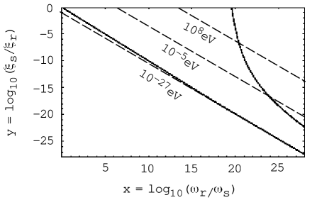
FIG. 2.: Possible allowed region for the parameters of an intermediate pre-big phase, consistent with an axion spectrum that does not become over-critical, and that reproduces the present COBE observations. The dashed lines represent curves of constant axion mass.

The allowed region is bounded by the bold solid curves. The lower border is fixed by the condition $m>H_{eq}\sim 10^{-27}$ eV for $x~{}\raise 1.72218pt\hbox{$>$}\kern-6.99997pt\lower 2.6694pt\hbox{$\sim$}~{}18$, and by the condition $\beta<1$, i.e. $y>-x$, for $x~{}\raise 1.72218pt\hbox{$<$}\kern-8.00003pt\lower 2.6694pt\hbox{$\sim$}~{}18$. The upper border is fixed by the condition $\Omega_{\sigma}(\omega_{m})<0.1$, imposed for $\omega_{T}>\omega_{s}$ and $m/H_{eq}>10^{16}$. The region is limited to the range $\omega_{r}/\omega_{s}~{}\raise 1.72218pt\hbox{$<$}\kern-8.00003pt\lower 2.6694pt\hbox{$\sim$}~{}10^{28}$, as we are considering the case in which the axion contribution to the CMB anisotropy arises from the low-frequency branch of the spectrum.

The dashed lines of Fig. 2 represent curves of constant axion mass, determined by the conditions (73), (75), with $g_{r}=10^{-2}$, $|r|=1.45$ and $T_{m}=100$ MeV, namely

$$y=-0.95x-0.9+{1\over 4}\log_{10}\left(m\over 10^{-27}{\rm eV}\right),~{}m<10^{-11}~{}{\rm eV},$$ (76)

$$y=-0.95x-4.9+{1\over 2}\log_{10}\left(m\over 10^{-27}{\rm eV}\right),~{}m>10^{-11}~{}{\rm eV}.$$ (77)

(78)

As shown in the picture, the allowed region is compatible with masses much higher than $H_{eq}$, up to the limiting value $m\sim 100$ MeV above which the discussion of this paper cannot be applied, since for $m>100$ MeV all the produced axions decayed into photons before the present epoch, at a rate $\Gamma\sim m^{3}/M_{p}^{2}$. For the particular example shown in Fig. 2, the allowed axion-mass window is then

$$10^{-27}~{}{\rm eV}<m<10^{2}~{}{\rm MeV}.$$ (79)

In the absence of the intermediate phase, i.e. for $x,y\rightarrow 0$, we recover the result obtained in [2], with $m\sim 10^{3.8}H_{eq}\sim 10^{-23}$ eV.

A high-curvature string phase with nearly constant dilaton and curvature scale, i.e. $\beta\simeq 1$, $y\simeq-x$, is not excluded but must lie very near the lower border of the allowed region, so that it does not relax in a significant way the bounds on the axion mass. It is nevertheless remarkable that such a phase is not inconsistent with axion production and with the COBE normalization of the axion spectrum. Such a phase would produce a relic gravity wave background with a nearly flat spectrum [27], easily observable by advanced detectors, and its extension in frequency would be constrained by $x~{}\raise 1.72218pt\hbox{$<$}\kern-8.00003pt\lower 2.6694pt\hbox{$\sim$}~{}18$, to avoid conflicting with present pulsar-timing data [29]. This does not introduce additional constraints in our discussion, however, since for $x>18$ the line $y=-x$ lies outside the allowed region of Fig. 2.

We conclude this section by giving a possible example of background, which satisfies the low-energy string cosmology equations, and which is simultaneously compatible with COBE and with higher values of the axion mass, as illustrated in Fig. 2.

Consider the gravi-dilaton string effective action, with zero dilaton potential, but with the contribution of additional matter fields (strings, membranes, Ramond forms, …) that can be approximated as a perfect fluid with an appropriate equation of state. As discussed in [30], the cosmological equations can in this case be integrated exactly, and the general solution is characterized by two asymptotic regimes. In the initial small-curvature limit, approaching the perturbative vacuum, the background is dominated by the matter sources. At late times, when approaching the high-curvature limit, the background becomes instead dilaton-dominated, and the effects of the matter sources disappear. The time-scale marking the transition between the two kinematical regimes (and thus the duration of the second, dilaton-dominated phase) is controlled by an arbitrary integration constant.

In order to provide an explicit example of this class of backgrounds, we can take, for instance, a $4+n$ manifold and we set

$$g_{\mu\nu}={\rm diag}\left(1,-a^{2}\delta_{ij},-b^{2}\delta_{mn}\right),$$ (80)

$$T_{\mu}^{\nu}={\rm diag}~{}\rho\left(1,-\gamma\delta_{i}^{j},-\epsilon\delta_{m}^{n}\right),$$ (81)

$$a\sim|t|^{\alpha_{1}},~{}~{}b\sim|t|^{\alpha_{2}},~{}~{}\phi=\Phi-n\ln b.$$ (82)

Here $\Phi$ is the unreduced, $(4+n)$-dimensional dilaton field and we have called $a$ and $b$, respectively, the external and internal scale factors, while $\gamma$ and $\epsilon$ define the external and internal equations of state. In the initial, matter-dominated regime ($\eta<\eta_{s}$), the string cosmology equations lead to [30]:

$$r={5\gamma-1\over 1+3\gamma^{2}+n\epsilon^{2}-2\gamma}-{1\over 2}.$$ (83)

In the subsequent dilaton-dominated regime ($\eta>\eta_{s}$) the equations give [31]

$$\beta={1-3\alpha_{1}\over 1-\alpha_{1}}-{1\over 2},~{}~{}~{}~{}\alpha_{1}^{2}={1\over 3}\left(1-n\alpha_{2}^{2}\right),$$ (84)

where $\alpha_{1},\alpha_{2}$ depend on $\gamma$, $\epsilon$, and on arbitrary integration constants.

The value $r=-3/2$, required for a flat low-frequency branch of the spectrum, is thus obtained provided internal and external pressures are related by:

$$n\epsilon^{2}=-3\gamma(1+\gamma).$$ (85)

On the other hand, an appropriate equation of state, motivated by the self-consistency of this background with the solutions of the string equations of motion [30, 32], suggests for $\gamma$ the range $-1/3\leq\gamma\leq 0$. This range, together with the condition (85), also guarantees the validity of the so-called dominant energy condition, $\rho\geq 0$, for the whole duration of the low-energy pre-big bang phase. Near the singularity, when the background enters the dilaton-dominated regime, the kinematics, and then the value of $\beta$, depends on the integration constants. For a particularly simple choice of such constants ($x_{i}=0$ in the notation of [30]), one finds $\alpha_{1}=\sqrt{-\gamma/3}$, and the value of $\beta$ becomes completely fixed by $\gamma$ as

$$\beta={1+\sqrt{-3\gamma}\over 1+\sqrt{-\gamma/3}}-{1\over 2}.$$ (86)

With $\gamma$ ranging from $-1/3$ to $0$, $\beta$ ranges from $-1/2$ to $1/2$. It is thus always possible, even in this simple example, to implement the condition $\beta<1$, in such a way as to satisfy the properties required by the allowed region of Fig. 2.

V Conclusion

In this paper we have discussed, in the context of the pre-big bang scenario, the possible consistency of a pseudoscalar origin of the large-scale anisotropy, induced by the fluctuations of non-relativistic Kalb–Ramond axions, with masses up to the $100$ MeV range. The enhancement of the low-energy tail of the axion spectrum, due to their mass, has been shown to be possibly balanced by the depletion induced by a steeper slope at high frequency. We have provided an explicit example of background that satisfies the low-energy string cosmology equations, and leads to an axion spectrum compatible with the above requirements.

The discussion of the reported example is incomplete in many respects. For instance, the class of models that we have considered could be generalized by the inclusion of additional cosmological phases; also, an additional reheating subsequent to the pre-big bang $\rightarrow$ post-big bang transition could dilute the produced axions, and relax the critical density bound; and so on. In this sense, the results discussed in Sect. IV are to be taken only as indicative of a possibility.

In this spirit, the main message of this paper is that in the context of the pre-big bang scenario there is no fundamental physical obstruction against an axion background that fits consistently the anisotropy observed by COBE, with “realistic” masses in the expected range of conventional axion models [8] –[12].

For a given axion mass, the corresponding anisotropy is only a function of the parameters of the pre-big bang models. If the axion mass were independently determined, the measurements of the CMB anisotropy might be interpreted, in this context, as indirect observations of the properties of a very early cosmological phase, and might provide useful information about the high-curvature, strong-coupling regime of the string cosmology scenario.

- [1]
- [2] R. Durrer, M. Gasperini, M. Sakellariadou and G. Veneziano, Seeds of large-scale anisotropy in string cosmology, gr-qc/9804076.
- [3] R. Durrer, M. Gasperini, M. Sakellariadou and G. Veneziano, Massless (pseudo-)scalar seeds of CMB anisotropy, astro-ph/9806015.
- [4] G.F. Smoot and D. Scott, in L. Montanet et al., Phys. Rev. D 50, 1173 (1994) (update 1996).
- [5] A. J. Banday et al., Astrophys. J. 475, 393 (1997).
- [6] E. J. Copeland, R. Easther and D. Wands, Phys. Rev. D 56, 874 (1997); E. J. Copeland, J. E. Lidsey and D. Wands, Nucl. Phys. B 506, 407 (1997).
- [7] R. C. Ritter et al., Phys. Rev. D 42, 977 (1990).
- [8] K. Kim, Phys. Rev. Lett. 43, 103 (1979); M. Dine, W. Fischler and M. Srednicki, Phys. Lett. B 104, 199 (1981).
- [9] S. Weinberg, Phys. Rev. Lett. 40, 223 (1978); F. Wilczeck, ibid, p. 279.
- [10] J. Preskill, M. Wise and F. Wilczeck, Phys. Lett. B 120, 127 (1983); L. M. Abbott and P. Sikivie, ibid 40, p.133; M. Dine and W. Fischler, ibid, p. 139.
- [11] R. Davis, Phys. Lett. B 180, 225 (1986); D. Harari and P. Sikivie, Phys. Lett. B 195, 361 (1987); A. Vilenkin and T. Vachaspati, Phys. Rev. D 35, 1138 (1987).
- [12] See for instance P. Sikivie, Int. J. Mod. Phys. D 3 Suppl., 1 (1994).
- [13] M. Axenides, R. H. Brandenberger and M. S. Turner, Phys. Lett. B 1260, 178 (1983); D. Seckel and M. S. Turner, Phys. Rev. D 32, 3178 (1985); Y. Nambu and M. Sasaki, Phys. Rev. D 42, 3918 (1990).
- [14] E. W. Kolb, A. Singh and M. Srednicki, Quantum fluctuations of axions, hep-ph/9709285.
- [15] G.Veneziano, Phys. Lett. B265,287 (1991); M. Gasperini and G. Veneziano, Astropart. Phys. 1, 317 (1993); an updated collection of papers on the pre-big bang scenario is available at http://www.to.infn.it/~gasperin/
- [16] V. F. Mukhanov, A. Feldman and R. Brandenberger, Phys. Rep. 215, 203 (1992).
- [17] V. Kaplunowsky, Phys. Rev. Lett. 55, 1036 (1985).
- [18] R. Brustein, M. Gasperini and G. Veneziano, Duality in cosmological perturbation theory, Phys. Lett. B (1998) (in press).
- [19] R. Brustein and H. Hadad, Phys. Rev. D 57, 725 (1998).
- [20] M. Gasperini, Phys. Lett. B 327, 215 (1994); M. Gasperini and G. Veneziano, Phys. Rev. D. 50, 2519 (1994).
- [21] R. Durrer and M. Sakellariadou, Phys. Rev. D 56, 4480 (1997).
- [22] R. K. Sachs and A. M. Wolfe, Ap. J. 147, 73 (1967).
- [23] J. E. Lidsey, A. R. Liddle, E. W. Kolb, E. J. Copeland, T. Harreiro and M. Abney, Rev. Mod. Phys. 69, 373 (1997).
- [24] M. Gasperini, Relic gravitons from the pre-big bang: what we know and what we do not know, in “String theory in curved space times”, ed. N. Sanchez (World Scientific, Singapore, 1998), p. 333.
- [25] A. Buonanno, K. A. Meissner, C. Ungarelli and G. Veneziano, JHEP01, 004 (1998).
- [26] M. Gasperini, M. Giovannini and G. Veneziano, Phys. Rev. Lett. 75, 3796 (1995).
- [27] R. Brustein, M. Gasperini, M. Giovannini and G. Veneziano, Phys. Lett. B 361, 45 (1995).
- [28] M. Gasperini, M. Maggiore and G. Veneziano, Nucl. Phys. B 494, 315 (1997).
- [29] V. Kaspi, J. Taylor and M. Ryba, Ap. J. 428, 713 (1994).
- [30] M. Gasperini and G. Veneziano, Phys. Rev. D 50, 2519 (1994).
- [31] G. Veneziano, Ref. [15].
- [32] M. Gasperini, M. Giovannini, K. A. Meissner and G. Veneziano, Evolution of a string network in backgrounds with rolling horizons, in “String theory in curved space times”, ed. N. Sanchez (World Scientific, Singapore, 1998), p. 49.