Hard-scattering factorization with heavy quarks: A general treatment

Abstract

A detailed proof of hard-scattering factorization is given with the inclusion of heavy quark masses. Although the proof is explicitly given for deep-inelastic scattering, the methods apply more generally. The power-suppressed corrections to the factorization formula are uniformly suppressed by a power of $\Lambda/Q$, independently of the size of heavy quark masses, $M$, relative to $Q$.

I Introduction

A correct treatment of heavy quarks in higher-order perturbative QCD calculations is important F2c ; photo ; Gluck.Reya ; DEN ; had.heavy ; ACOT ; other ; BMSvN ; MRRS ; RT2 ; RT1 to precision phenomenology. Among the reasons is the fact that a substantial fraction of the deep-inelastic cross section at HERA is in heavy quark production. Moreover, this occurs in a region where the heavy quark masses are not necessarily negligible with respect to the large momentum scales in the problem (like $Q$).

However, there is a considerable confusion Gluck.Reya ; ACOT ; other ; BMSvN ; MRRS ; RT2 ; RT1 about what constitute correct methods for treating heavy quarks. Some of the difficulties occur because many treatments assume that quarks either are so light that their masses are negligible with respect to $Q$ or have masses that are of order $Q$, where $Q$ denotes a typical scale for the hard-scattering process under discussion. One has to be able to handle the intermediate region, where $Q$ is somewhat larger than a quark mass but not enormously much larger.

Even when $Q$ is much larger than all quark masses, the intermediate region must still be treated, because evolution equations are used to obtain the strong coupling, the parton densities, and the fragmentation functions from starting values specified at scales of a few GeV. The symptoms of this issue are the different and apparently incompatible “matching conditions” that have been proposed.

In this paper I will give a relatively simple and general proof of factorization including the effects of heavy quarks. The only issue that will not be treated is the cancellation of soft gluons, an issue which is essentially orthogonal to the ones which are causing problems. The key ingredient is the observation that the short-distance coefficient functions (“Wilson coefficients”) can legitimately be calculated with the quark masses left non-zero. Previous work with Aivazis, Olness and Tung ACOT and others other has used this method; what is new is the complete and detailed all-orders proof.

This first main characteristic of the method, that quark masses are retained when necessary in the calculations of the coefficient functions, enables factorization to be valid when the masses of quarks are non-negligible with respect to the large scale $Q$ of the hard scattering. Hence the method avoids the normal problem when the $\overline{{\rm MS}}$ scheme is used with massless Wilson coefficients, that there are uncontrolled corrections of order a power of $M/Q$, where $M$ is a heavy quark mass.

The second main characteristic is that the renormalization and factorization scheme consists of a series of subschemes labeled by the number of “active quark flavors”, $n_{A}$. This is simply a generalization of the Collins, Wilczek and Zee (CWZ) scheme CWZ that is in standard use PDG for the QCD coupling $\alpha_{s}$. When discussing the numerical values of parton densities, it is necessary to specify the number of active flavors that is used in their definition, just as in the case of the coupling.

The subschemes with different numbers of active flavors are useful in different ranges of physical scales, but with overlapping ranges of validity. Since the subschemes are related by definite matching conditions coupling-match ; pdf-match , the choice of the number of active flavors does not result in any more indefiniteness in the physical predictions than does the freedom to choose a scheme or a value of the renormalization/factorization scale.

At first sight, the use of a sequence of subschemes instead of a single scheme appears rather baroque. However, it is in fact the simplest implementation of mass-dependent factorization perfect . We require that the schemes implement decoupling AC of heavy quarks when appropriate, and that they implement the closest possible scheme to the mass-independent $\overline{{\rm MS}}$ scheme, which is commonly used for most perturbative QCD calculations. If one did not have a sequence of schemes, it would be necessary to have mass-dependent evolution equations. The CWZ scheme does have mass-dependent evolution in the following sense. If one chooses particular “thresholds”—more accurately called “switching points”—to change the number of active flavors, then the evolution kernels change at the thresholds. Moreover, the matching conditions at the thresholds can be thought of as corresponding delta-function contributions to the kernels.

Some of the confusion in the literature can be traced to the supposition that Wilson coefficients must be calculated with massless quarks. Indeed, many papers, for example BMSvN ; CFP ; Ellis.et.al , treat factorization as a question of factoring out mass divergences in a massless theory. Such methods founder when the quarks have non-negligible masses, since then some of the divergences are not literally present. It should be noted that the proof of factorization in CSS does not assume that quarks are massless (contrary to the assertion in RT1 ); the proof merely assumes that one is treating a limit in which the scale of the hard scattering is much larger than all masses.

Another source of problems is that many treatments of factorization BMSvN ; CFP ; Ellis.et.al take as their starting point an assertion that hard cross sections are the convolution of “bare parton densities” with unsubtracted “partonic cross sections”. Although this assertion is widespread, it has no proof: it has the status of an unproved conjecture. Indeed it is not obvious that it is even true. However, this bare parton conjecture is not necessary either to the proof of the factorization theorem or to its use.

These problems with existing treatments, even without the treatment of heavy quarks, provide motivation for providing much detail in the proofs in this paper. The proofs apply equally well in the absence of heavy quarks.

The treatment in this paper will be based on the basic power counting theorems derived by Libby and Sterman LS and on the methods of Curci, Furmanski and Petronzio CFP for organizing sums of generalized ladder graphs. The treatment of heavy quarks uses the methods of Collins, Wilczek and Zee (CWZ) CWZ . The powerful methods developed by Chetyrkin, Tkachov, and Gorishnii perfect ; CTG ; AsyOp for the operator product expansion with mass effects are consistent with the CWZ scheme.

The outline of this paper is as follows: In Sec. II, I explain the requirements that I consider necessary to impose on a good treatment of mass effects. Then, in Sec. III, I review the CWZ scheme for renormalization. In that section, I also define a consistent terminology of “light” and “heavy” quarks, and of “partonic” (or “active”) and “non-partonic” quarks. In Secs. IV to IX, I prove factorization in the case that there is one heavy quark and that $Q$ is at least as large as the heavy quark mass; this is the case where the heavy quark is active. As an interlude in the formal proof, in Sec. VI, I provide a mathematical example of the asymptotics of certain integrals that mimic the behavior of the more complicated integrals in Feynman graphs for QCD. Then in Sec. X, I prove factorization for the case that the heavy quark may be treated as inactive. (“Non-partonic” is a better term.) The general case, that there are several heavy quarks of various masses, forms a relatively simple generalization of the preceding work, and is treated in Sec. XI. An account of the matching conditions and of the evolution equations is given in Sec. XII. This is followed by an account of the relation of the present scheme to the schemes of other authors, in Sec. XIII. The conclusions are in Sec. XIV. In the Appendix, I explain a certain mathematical complication that appears in the middle of the proof.

II Requirements for a good factorization scheme

The overall aim of work such as ours is to represent interesting cross sections (or other quantities) in terms of perturbatively calculable quantities and a limited set of non-perturbative quantities that must at present be obtained from experiment. A typical result is that for deep-inelastic structure functions and other hard-scattering cross sections we have factorization theorems: the leading large $Q$ behavior is a convolution of hard-scattering coefficients, which can be perturbatively calculated, and of parton densities and/or fragmentation functions. There are also evolution equations for the parton densities, etc., for which the evolution kernels are perturbatively calculable.

Although the factorization theorems are true in a general quantum field theory, and not just in QCD, their particular utility in QCD is caused by the asymptotic freedom of QCD. Without the use of factorization, perturbative calculations of typical scattering amplitudes and cross sections involve integrals down to low virtualities where the effective coupling is too large for low-order perturbation theory to be valid. Factorization theorems segregate the non-perturbative part of a cross section into a limited number of experimentally measurable parton densities, etc. Moreover, typical cross sections depend on several scales and perturbative calculations typically have one or two logarithms of ratios of scales for each loop. Since the QCD coupling is not very small, the logarithms can ruin the accuracy of practical calculations. By working with quantities that each depend on a single scale, one avoids this loss of accuracy.

For the purposes of this section, we will let $Q$ be a (large) scale defining the kinematics of the hard-scattering process under discussion and we will let $M$ denote the mass of some heavy quark. A satisfactory treatment should satisfy the following requirements:

1. The formalism should apply to all orders of perturbation theory and include arbitrarily non-leading logarithms.

2. Explicit definitions must be given of the non-perturbative quantities, as matrix elements of operators.

3. The formalism is to be applicable to all the cases $Q\gg M$, $Q\sim M$ and $Q\ll M$, and the errors are suppressed by a power of $\Lambda/Q$.

4. Multiple heavy quarks should be treated without loss of accuracy no matter whether the ratios of the masses are large or not.

The results in this paper will also satisfy some other requirements which are more matters of convenience than absolute principles:

1. When a quark mass is large enough for decoupling to apply, calculations should exhibit manifest decoupling. That is, they should reduce to calculations in a standard scheme (e.g., $\overline{{\rm MS}}$) in the theory with the heavy quarks omitted, and with no need to adjust the numerical values of the coupling.

2. The scheme should reduce to a standard scheme (e.g., $\overline{{\rm MS}}$) when the masses are much less than $Q$. We will in fact use the $\overline{{\rm MS}}$ scheme, so that standard hard-scattering calculations can be used unchanged in the case that masses can be neglected.

3. The previous two requirements apply to both factorization and to the coupling $\alpha_{s}$.

4. The evolution equations for the parton densities, etc., should be homogeneous. That is, they should be of the form of conventional DGLAP equations or renormalization group equations rather than of the form of Callan–Symanzik equations Callan.Symanzik . (The solutions of Callan–Symanzik equations need an extra level of approximation to make them useful for calculations.)

III CWZ scheme

The short-distance coefficient functions are almost completely determined once one has specified a scheme for defining the parton densities — in fact a scheme for renormalizing the ultra-violet divergences in the coupling and in the parton densities. The scheme defined in this paper is in fact a composite of a series of related schemes in the fashion proposed by Collins, Wilczek and Zee (CWZ) CWZ .

First, it is necessary to introduce some terminology whose consistent use will aid our work. Let us define a “light” quark or gluon to be one whose mass is of the order of $\Lambda$ or less, i.e., under about a GeV. Similarly, let us define a “heavy” quark to be one whose mass is larger than a GeV or so, so that the the effective coupling, $\alpha_{s}(M)$, at the scale of a heavy quark mass is in the perturbative region. With this definition, the charm, bottom and top quarks are the heavy quarks. We let $n_{l}$ be the number of light quarks, and $n_{f}$ be the total number of quarks. In our present state of knowledge of QCD we have $n_{l}=3$ and $n_{f}=6$.

Each subscheme of the CWZ scheme is labeled by a number $n_{A}$, which I will call the number of “active” (or “partonic”) quarks. These are the $n_{A}$ lightest quarks. All the remaining quarks I call “non-partonic”. (It is also possible to call them “inactive”, but the term can be misleading.) In each subscheme:

1. Graphs that contain only active parton lines (i.e., gluons and active quarks) are renormalized by $\overline{{\rm MS}}$ counterterms, with the exception of the renormalization of the masses of heavy quarks.

2. Graphs all of whose external lines are active partons but which have internal non-partonic quark lines are renormalized by zero-momentum subtraction.

3. Heavy quark masses are defined as pole masses, as in the work of Smith, van Neerven and collaborators F2c ; photo ; BMSvN . (We could also to choose to define heavy quark masses as $\overline{{\rm MS}}$ without changing the formalism.)

4. Other graphs with external non-partonic lines are renormalized by $\overline{{\rm MS}}$ counterterms.

These definitions are applied to the renormalization of the interaction and to the renormalization of the parton densities, fragmentation functions, etc.

A consequence of the definitions is that we will talk about “three-flavor”, “four-flavor”, etc., definitions of the coupling and parton densities (and fragmentation functions). Use of such a sequence of definitions is already common practice for the coupling PDG , and identical considerations apply to the parton densities. As a consequence it is meaningful to specify numerical values of the coupling and of parton densities only if the number of active flavors is specified. There are perturbatively calculable relations, or matching conditions, between the values of these quantities with different numbers of active flavors.

I will now list properties of this set of schemes that are important for our purposes. Their proofs are either in Ref. CWZ or are later in this paper.

1. The scheme coincides with ordinary $\overline{{\rm MS}}$ when all partons are active, i.e., $n_{A}=n_{f}$.

2. Manifest decoupling is obeyed. If we have a process in which all external momentum scales are much less than the masses of the non-partonic quarks, then we can omit all graphs containing non-partonic quarks and only make a power-suppressed error. In contrast, in a scheme that does not have manifest decoupling, we would have to adjust the numerical values of the couplings and of the parton densities.

3. Evolution equations for the densities of active partons and of the coupling $\alpha_{s}$ are exactly those of a pure $\overline{{\rm MS}}$ scheme in a theory with $n_{A}$ quark flavors. This is a consequence of the mass-independence of UV counterterms in the $\overline{{\rm MS}}$ scheme, together with an application of the decoupling theorem AC ; Witten .

4. The relation between the subschemes is just a particular case of the relation between different renormalization schemes. The matching conditions between the schemes with different numbers of active quarks are known to three loops for the coupling coupling-match and to two loops for the parton densities pdf-match . The matching conditions between quantities in the subschemes with $N$ and $N+1$ active flavors involve no large logarithms of masses, provided that the renormalization/factorization scale $\mu$ is of order the mass of the $(N+1)$th quark. (For example, we would choose $\mu$ to be of order the mass of the mass of the charm quark when we compute the relation between the three- and four-flavor schemes.)

5. In general, if one varies the physical scale $Q$ of some process (e.g., deep-inelastic scattering), one should vary the number of active quarks suitably. Quarks of mass much less than $Q$ are to be active, while quarks of mass much larger than $Q$ should be non-partonic. One has a choice for those flavors whose masses are close to $Q$, and I suspect a bias in favor of keeping quarks non-partonic will lead to more accurate calculations.

6. The light partons are always to be treated as active.

It might be considered odd that in a region where $Q$ is of the order of the mass of some heavy quark we have a choice as to whether to treat the quark as active or not. The freedom is entirely comparable to the freedom to choose the precise value of the renormalization/factorization scale. Indeed the existence of a region where the two subschemes have comparable accuracy is vital to the success of a good treatment of heavy quarks, because it enables reliable perturbative calculations to be made of the matching conditions coupling-match ; pdf-match between the two subschemes.

Commonly ACOT ; RT2 ; PDG , the scheme is implemented by choosing what can be called “matching” and “switching” points to be equal to the relevant heavy quark mass. For example, in treating DIS with a charm quark, one often sets the renormalization/factorization scale $\mu$ to the kinematic variable $Q$. Then one uses a 3-flavor subscheme if $\mu<m_{c}$ and a 4-flavor subscheme if $\mu>m_{c}$. One also chooses to evaluate the matching conditions between the subschemes at $\mu=m_{c}$. None of these choices is essential, and any change gives a change in the physical predictions only because of the errors due to the truncation of the perturbation series. It is probably only appropriate (i.e., suitable for fixed order perturbative calculations) to use a 4-flavor subscheme if one is treating a situation where the cross section is above the physical threshold for charm production, which is at $Q=2m_{c}\sqrt{x/(1-x)}$. Hence, if $x$ is rather large, then it would be appropriate to use the 3-flavor scheme even when $Q$ is substantially above $m_{c}$.

Note that there are three distinct mass scales referred to in the previous paragraph: a matching point, a switching point and a physical threshold.

Of course, one is free to disregard the CWZ scheme and use some other scheme, provided that it provides complete definitions of the parton densities and of the coupling. However, this does not affect the validity of the CWZ definitions. The significance of the CWZ definitions is that when all flavors are active, they are exactly the $\overline{{\rm MS}}$ ones.

IV Basics of factorization when $Q\gtrsim M$

The principles of the proof can be best explained by first considering the case that there is exactly one heavy quark, of mass $M$. There will be in effect two factorization theorems to prove. The first, whose treatment starts in this section, is appropriate when the physical scale $Q$ of the hard scattering is at least at large in magnitude as $M$. In this case, it is appropriate to treat the heavy quark as active: the factorization theorem will include a term with a heavy quark density.

The second case, whose treatment starts in Sec. X, is appropriate when $Q\lesssim M$, and it treats the heavy quark as non-partonic. Then the factorization theorem has no term with a heavy quark density, and all heavy-quark production is to be found (at leading power) in the coefficient function.

As mentioned earlier, there is an overlap region, $Q\sim M$, where both theorems are appropriate, i.e., they give comparable accuracy in predictions based on finite-order calculations of coefficient functions.

So in this section, we start the treatment of a factorization theorem for deep-inelastic structure functions, given the assumption that $Q\gtrsim M$. A single factorization formula will cover the case that $Q$ is much bigger than the heavy quark mass, as well as the case that $Q$ and the heavy quark mass are comparable, and the intermediate region. Our notation for the photon momentum $q$, the hadron momentum $p$, and for the Bjorken variable $x$ is standard. As usual $Q^{2}=-q^{2}>0$. We will assume that quark masses are at most of order $Q$.

When reading through the proof, it may be worth the reader’s while to refer ahead to Sec. VI. There, a simple mathematical example is given of the kinds of integral under discussion, and it is possible to see more easily the meaning of the formal manipulations in the proof.

IV.1 Leading regions

In the Bjorken limit (large $Q$, fixed $x$), the leading power behavior is given by the regions symbolized in Fig. 1, as was proved by Libby and Sterman LS ; Sterman.TASI95 . In each region, there is what we call a hard subgraph $H$, all of whose lines are effectively off shell by order $Q^{2}$. It is to this subgraph that the virtual photons couple. The rest of the graph has lines that are much lower in virtuality and that are approximately collinear to the momentum $p$ of the target. The latter part of the graph we will call the target subgraph $T$. We will give more quantitative characterizations of the regions later. (For example, we must deal with the fact that there is a final-state cut, so that some lines in $H$ are actually on shell instead of having virtuality $Q^{2}$.)

Although one often does purely perturbative calculations in which the target is a quark or gluon state, our treatment will also apply to hadron targets. In that case, suitable bound-state wave functions will be incorporated in $T$.

Figure 1: Regions for the leading power of structure functions have this structure.

A result of the power counting is that for a contribution to have the leading power — to be of “leading twist” — the two subgraphs $H$ and $T$ must be connected to each other by two parton lines, one on each side of the final-state cut. The set of decompositions into two such subgraphs $H$ and $T$ is in one-to-one correspondence with the set of leading regions. There are two exceptions to this correspondence. The main exception is that if the heavy quark mass is of order $Q$, then the $H$ and $T$ subgraphs are connected by light parton lines, but not by heavy quark lines. This exception arises because the definition of the region implies that the lines joining $H$ and $T$ have virtuality much less than $Q$, and this is not possible if the lines are heavy quark lines of a mass comparable to $Q$. The second exception to the power-counting rules is that gluons with scalar polarization can couple the $H$ and $T$ subgraphs without a power-law penalty, at least in a covariant gauge: we will discuss this issue in more detail later in the section.

We define the subgraph $T$ to include the full propagators of the lines joining it to $H$, since these lines have momenta collinear to the target. Hence the hard subgraph $H$ is one-particle-irreducible (1PI) in these same lines.

In this and later figures, we have the initial state at the bottom of the graph, and the hard subgraph to the left. This ensures that the orientation of the figures corresponds to the equations we will write for convolutions of amplitudes. For example, we can write Fig. 1 as $H\cdot T$.

Any region of loop-momentum space that cannot be characterized by Fig. 1 is suppressed by a power of $Q$. Therefore the statement that the leading regions have the form of Fig. 1 is true to all orders in the coupling and includes not just the leading logarithms but all non-leading logarithms as well.

A typical graph can have many different decompositions into hard and target subgraphs. For example, Fig. 2 has four such decompositions, and hence four leading regions. The possibility of having more than one leading region is characteristic not only of QCD, but of any renormalizable field theory, since adding extra lines inside $H$ in a theory with a dimensionless coupling does not change the counting of powers of $Q$. It is the large multiplicity of regions that results in many of the complications in the proof of factorization. In addition, it results in the logarithmic dependence on $Q$ that is typical of higher order calculations in QCD.

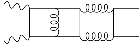
Figure 2: A graph with 4 decompositions of the form of Fig. 1.

In contrast, super-renormalizable theories (e.g., QCD in less than four space-time dimensions) have couplings with positive mass dimension. This implies that there is a single leading region. It is of the form of Fig. 1, but with the smallest possible graph for $H$. That is, the unique leading region has the form of the handbag diagram, Fig. 3. Although super-renormalizable theories do not represent real strong-interaction physics, experience in treating simple cases is useful in formulating the factorization theorem. Factorization, etc., for super-renormalizable theories is equivalent to the set of results obtained many years ago by Landshoff and Polkinghorne in the context of their covariant parton model LP .

Figure 3: The handbag diagram that characterizes the only leading region in a super-renormalizable theory.

Let us now list some technical complications that we will be able to ignore, but that are treated in other papers LS ; CS ; CSS on factorization:

1. Although we have defined the target part $T$ to consists only of lines with collinear momenta, it may in fact contain some highly virtual lines. These are confined to subgraphs that are ultra-violet divergent and just generate the usual UV divergences that are canceled by counterterms in the Lagrangian. This complication does not affect our proofs, since none of the divergent subgraphs in QCD overlap between $T$ and $H$, and our proofs will treat $T$ as a black box.

2. Although we treat the hard subgraph as being composed of lines all of which have large virtuality, this subgraph necessarily includes at least one final-state line. But after a sum over the possible final-state cuts, the hard subgraph is a discontinuity of a certain Green function. Then LS the whole graph can be represented as a contour integral over a Green function in which all the lines in $H$ are off shell by order $Q^{2}$. Thus $H$ can indeed be treated as if its lines are all far off shell. In particular, light-quark masses can legitimately be neglected compared to $Q$. A simple example is given by a super-renormalizable theory. Graphs with cut and uncut propagator corrections, Fig. 4, to the handbag diagram have the same power law in $Q$ as the simple handbag diagram. Such graphs generate the correct final-state hadrons for the current-quark jet. After a sum over cuts, all such corrections cancel at the leading power of $Q$, and the structure function is correctly given by the lowest order handbag Fig. 3.

3. Soft gluons can connect the different final-state jets, and can connect the final-state jets to the target subgraph. After a sum over final-state cuts these contributions cancel. This complication is only present in a theory with elementary vector fields, e.g., QCD. A cancellation can be proved, and for the purposes of this paper, we may assume that no complications result from the implementation of the cancellation of soft gluons. In more general processes, like the Drell-Yan process, the issue of soft-gluon cancellation is much more difficult CS ; CSS .

4. In a general gauge, there can be extra collinear gluon lines connecting $T$ and $H$. Such gluons only contribute to the leading power if they have scalar polarization. However, if a suitable “physical” gauge is used (e.g., axial gauge with a gauge fixing vector proportional to $q$), such contributions are not present LS . There are some subtleties associated with the use of such a gauge. For example, the analysis of the leading regions in Refs. LS ; Sterman.TASI95 relies critically on Landau’s analysis of the singularities associated with the denominators of Feynman propagators. But physical gauges introduce extra unphysical singularities — the physical gauges are not as physical as one often supposes. For the purposes of this paper it is sufficient to ignore this complication, or to assume that the appropriate light-like gauge is being used.

5. The same phenomenon (in a covariant gauge) leads to what I term “super-leading” contributions, when $H$ and $T$ are joined only by gluons that have scalar polarizations. It can be shown scalar-polarization that the super-leading contributions cancel after a sum over a “gauge-invariant set” of graphs for $H$, and that CSS ; scalar-polarization the sum over attachments of scalar gluons to the hard part gives the correct gauge-invariant form of the parton densities, with a path-ordered exponential of the gluon field joining the two main parton vertices.

Figure 4: Handbag diagram with the final-state interactions that make the current quark jet.

IV.2 Relation of leading regions to mass singularities

To characterize the regions of momenta that Fig. 1 depicts, it is convenient to use light-front coordinates, where we write a 4-vector $V$ as $V^{\mu}=(V^{+},V^{-},{\bf V}_{T})$ with $V^{\pm}=(V^{0}\pm V^{z})/\sqrt{2}$. Then we choose a coordinate frame such that

$$p^{\mu} = \left(p^{+},\frac{m_{p}^{2}}{2p^{+}},{\bf 0}_{T}\right),$$

$$q^{\mu} \approx \left(-xp^{+},\frac{Q^{2}}{2xp^{+}},{\bf 0}_{T}\right).$$ (1)

The approximation in the definition of $q$ represents the neglect of power suppressed terms, given that $x$ is normally defined as $Q^{2}/2p\cdot q$.

To exhibit the counting of powers of $Q$ in its simplest form, we will choose to boost the frame in the $z$ direction until $p^{+}$ is of order $Q$. Then regions of momentum corresponding to the hard and target subgraphs are defined by saying that, for a momentum $k^{\mu}$,

• $k$ is in $H$ if $k^{-}$ is of order $Q$.

• $k$ is in $T$ if $k^{\mu}=\left(O(Q),o(Q),o(Q)\right)$, i.e., $k^{+}$ is of order $Q$, while $k^{-}$ and $k_{T}$ are much smaller than $Q$, as is appropriate for a momentum collinear to the incoming hadron.

After a sum over final-state cuts, the interactions that hadronize the jets in the hard subgraph cancel LS ; Sterman.TASI95 , and then we may treat the lines in $H$ as if they are all off shell by order $Q^{2}$.

The gauge we are using is the light-cone gauge $A^{+}=0$. In this gauge, regions with extra gluons joining the target and hard subgraphs in Fig. 1 are power suppressed.

Much of the literature treats factorization in terms of mass singularities. To see the relation to our treatment, suppose that we were to take a limit of the structure function in which all light quarks and all external lines are massless. The target momentum would become light-like: $p^{\mu}\to(p^{+},0,{\bf 0}_{T})$, so that there would be collinear and infra-red divergences. The infra-red divergences cancel after a sum over the different possible graphs and final-state cuts at a given order of perturbation theory, leaving only the collinear divergences associated with the target. These occur Sterman.TASI95 at momentum configurations symbolized again by Fig. 1, but where momenta in $T$ are exactly proportional to the target momentum, i.e., they are of the form $k^{\mu}=(k^{+},0,{\bf 0}_{T})$. There is an exact correspondence between the leading regions (for any $m$) and the location of the singularities for $m=0$: the leading regions are just neighborhoods of the positions of the singularities. Moreover the counting of powers of $Q$ corresponds to the degree of divergence of the singularities.

However, in the true theory there need not be any actual divergences. For example, in a non-QCD model we could endow all the particle with masses, and our proof of factorization would remain correct. In QCD there are divergences that are associated with the necessary masslessness of the gluon, but only if we make perturbative calculations with on-shell external gluons or quarks. In the real world, these divergences are cut off by the non-perturbative effects of confinement. All the real particles of QCD are massive. The singularities in the massless limit merely provide a convenient tool for classifying regions of momentum space.

IV.3 Elementary treatment of factorization

The factorization theorem can easily be motivated from Fig. 1, as we will now show. We will construct an approximation to a proof of the theorem that will introduce a number of useful ideas. The proof will be exactly correct in a super-renormalizable theory, where the single important region is given in Fig. 3. In that case the proof is equivalent to the argument given by Landshoff and Polkinghorne for the parton model LP . The greater detail given in the present paper will enable us to make precise operator definitions of parton densities. In addition, we will introduce some notations and auxiliary concepts that will be useful in the full proof.

The hypothesis on which the approximate proof rests is an assumption that important momenta can be classified as belonging to either a region of hard momenta (that belong only in $H$) or a region of momenta collinear to the initial hadron $p$ (that belong only in $T$). We will need to assume (not quite correctly) that the momenta collinear to the target have virtualities that are fixed when $Q$ becomes large, and more specifically that the orders of magnitude of the components of a target momentum are $(Q,m^{2}/Q,m)$, where $m$ is a typical light hadron scale.

Given this hypothesis, each graph can be decomposed unambiguously into a sum of terms of the form of Fig. 1. Thus we can write

$$F = \sum_{{\rm graphs}\ \Gamma}\Gamma+\mbox{non-leading power}$$ (2)

$$= \sum_{{\rm graphs}\ \Gamma}\ \sum_{{\rm regions}\ R}H(R)\cdot T(R)+\mbox{non-leading power},$$

where the summation over $\Gamma$ is restricted to those graphs that are two-light-particle reducible in the $t$-channel and that therefore have at least one decomposition of the form of Fig. 1. A region of such a graph is completely defined by its hard and target subgraphs, so we can replace the sum over graphs and regions by independent sums over graphs for $H$ and $T$:

$$F=H\cdot T+\mbox{non-leading power}.$$ (3)

Here $H$ and $T$ are the sum over all possibilities for the $H$ and $T$ subgraphs in Fig. 1, with the momenta being restricted to the appropriate regions. The symbol $\cdot$ represents a convolution, the integral over the 4-momentum linking $H$ and $T$ and a sum over the flavor, color and spin indices of the lines joining the two subgraphs. Thus we have

$$H\cdot T=\sum_{i}\int\frac{d^{4}k}{(2\pi)^{4}}\,H_{i}(q,k)\,T_{i}(k,p).$$ (4)

Recall that we defined $T$ to include the full propagators on the two lines that connect it to $H$, so that $H$ is amputated in these same two lines.

To get the factorization theorem, we use the observation that some of the components of the loop momentum can be neglected in $H$, and also that some of the components of the trace over spin labels can be neglected. In the $H$ factor in Eq. (4), we may neglect both $k^{-}$ and $k_{T}$, since all the lines in $H$ are effectively off shell by order $Q^{2}$. This results in an error that is suppressed by one or two powers of $Q$. Thus we can approximate the structure function by:

$$F=\int_{x}^{1}\frac{d\xi}{\xi}H\left[q,(\xi p^{+},0,{\bf 0}_{T})\right]\int\frac{dk^{-}\,d^{2}{\bf k}_{T}}{(2\pi)^{4}}\xi p^{+}T(k,p)+\mbox{non-leading power}.$$ (5)

Here, to make contact with the standard usage in this subject, we have written $k^{+}=\xi p^{+}$ and have changed variable from $k^{+}$ to $\xi$.

In Eq. (5) there is an implicit sum over the spin indices and the flavor of the lines joining $T$ and $H$. Suppose the line is a quark. Then we can decompose each of $H$ and $T$ into a sum of Dirac $\gamma$ matrices. The leading terms involve a $\gamma^{-}$ in the target subgraph $T$ since that can be contracted with the largest momentum components in $T$, which are the $+$ components. Thus the most general form of the part of $T$ that gives the leading power is a sum of terms proportional to $\gamma^{-}$, $\gamma^{-}\gamma_{5}$ and $\gamma^{-}{\bf\gamma}_{T}$.

For the simple case of unpolarized scattering, only the $\gamma^{-}$ term contributes, and we can write

$$F=\sum_{a}\int\frac{d\xi}{\xi}\mathop{\rm tr}H_{a}\gamma^{-}\int\frac{dk^{-}\,d^{2}k_{T}}{(2\pi)^{4}}\xi p^{+}\frac{1}{4}\mathop{\rm tr}\gamma^{+}T_{a}+\mbox{gluon terms}+\mbox{non-leading power},$$ (6)

with a similar decomposition being applied to the gluon term. Here $a$ labels the different flavors of quark and antiquark. (Note that in the usual applications, $H$ and $T$ are diagonal in quark flavor and only a single flavor index is required, the same for each of the lines joining $H$ and $T$.) A similar result applies when $H$ and $T$ are joined by gluon lines.

It is convenient to represent this formula in a convolution notation with the aid of a projection operator $Z$:

$$F=H\cdot Z\cdot T+\mbox{non-leading power}.$$ (7)

$Z$ represents the operation of setting $k_{T}=k^{-}=0$ for the momentum of the external parton of the hard scattering and of picking out the largest terms in the spin indices coupling the hard and target subgraphs. It is a sum of quark and gluon terms. The quark term is

$$Z_{\alpha\alpha^{\prime};\beta\beta^{\prime}}(k,l;\mbox{1st definition})=\frac{1}{4}\gamma^{-}_{\alpha\alpha^{\prime}}\gamma^{+}_{\beta\beta^{\prime}}\,(2\pi)^{4}\delta(k^{+}-l^{+})\delta(k^{-})\delta^{(2)}({\bf k}_{T}).$$ (8)

This and similar objects will be used repeatedly in our work. It is readily verified that $Z$ is a projection, i.e.,

$$Z^{2}=Z,$$ (9)

and hence, for example, $(1-Z)\cdot Z=0$. The label “1st definition” in Eq. (8) indicates that a modified definition, which we will now give, is superior.

In fact, the above definition of the projector $Z$ is suitable for massless quarks. Its use in Eq. (7) remains valid when the quarks in $H$ have non-zero mass, but it is not perfectly convenient for practical calculations. For example, calculations of the short-distance coefficient functions do not satisfy exact gauge invariance, because the external lines of $H$ are off shell. Therefore it is convenient to replace Eq. (8) by a definition in which the external quarks of $H$ are put on shell. This involves replacing $k$ by an on-shell momentum

$$\hat{k}^{\mu}=(\xi p^{+},m^{2}/2\xi p^{+},{\bf 0}_{T}),$$ (10)

and using the Dirac matrix for on-shell wave functions:

$$Z_{\alpha\alpha^{\prime};\beta\beta^{\prime}}(k,l;\mbox{massive quark})=\frac{\hat{k}_{\mu}\gamma^{\mu}_{\alpha\alpha^{\prime}}+m}{4k^{+}}\gamma^{+}_{\beta\beta^{\prime}}(2\pi)^{4}\delta(k^{+}-l^{+})\delta(k^{-}-m^{2}/2k^{+})\delta^{(2)}({\bf k}_{T}).$$ (11)

The resulting leading-power approximation to $F$ is

$$H\cdot Z\cdot T=\sum_{a}\int\frac{d\xi}{\xi}\mathop{\rm tr}H\frac{\hat{k}^{\mu}\gamma_{\mu}+m}{2}\int\frac{dk^{-}\,d^{2}{\bf k}_{T}}{(2\pi)^{4}}\mathop{\rm tr}\frac{\gamma^{+}}{2}T+\mbox{gluon terms}.$$ (12)

Here $\hat{k}^{\mu}$ is the approximated momentum, Eq. (10). Notice that although the external parton lines of $H$ are put on-shell, this is not true of the corresponding external partons of the target subgraph $T$; these are integrated over all values of $k^{-}$ and $k_{T}$ in the collinear region of momentum.

The change in the definition of $Z$ for massive quarks does not affect the factorization theorem (7). To see this, observe that the change of definition only changes small components of the momentum $k$ and of the $\gamma$ matrices attached to $H$. Thus we have only made an error similar in size to the power-suppressed error that we already induced by making an approximation in the first place. Also the algebraic property $Z^{2}=Z$, which we will make frequent use of later, is unchanged.

Since the operation $Z$ projects out the integral over $k^{+}$, Eq. (7) gives the structure function as a convolution of a hard-scattering coefficient and parton densities:

$$F=\hat{F}\otimes f+\mbox{non-leading power}.$$ (13)

The symbol $\otimes$ represents a convolution in the $\xi$ variable, together with a sum over quark flavors and over the gluon. It will also include a sum over the spin degrees of freedom if polarization-dependent effects are being treated.

The parton densities can be expressed in their usual form pdf.CS as matrix elements of light-cone operators. A quark density is then

$$f(\xi)=\int\frac{dk^{-}\,d^{2}{\bf k}_{T}}{(2\pi)^{4}}\mathop{\rm tr}\frac{\gamma^{+}}{2}T(k,p).$$ (14)

Given that we obtained the factorization theorem by decomposing momentum space into a hard region and a collinear region, the integral in Eq. (14) is restricted to the collinear region. When we provide a more correct proof, we will remove the restriction to collinear momenta, so that the definition of a parton density is exactly as a matrix element of a bilocal operator on the light-cone.

From the definition of $Z$, Eq. (11), it then follows that that the hard-scattering coefficient is computed from $H$ by contracting with the Dirac matrices appropriate for an external on-shell fermion, with a spin average:

$$\hat{F}=\mathop{\rm tr}H\frac{\hat{k}^{\mu}\gamma_{\mu}+m}{2}.$$ (15)

The factor of $1/2$ means that $\hat{F}$ has the normalization of a spin-averaged cross section.

IV.4 Why the simple derivation does not work

The above derivation of the factorization theorem would be valid if one could use a fixed decomposition of momentum space into regions appropriate for $H$ and $T$, at least up to power-suppressed terms. This assumption is in fact true in a super-renormalizable theory, and the above derivation then leads to the parton model. Only the lowest order graph for $H$ gives a leading contribution in this case, Fig. 3. This kind of reasoning led Feynman to formulate the parton model parton.model .

Unfortunately the error estimates obtained from the above argument, in a renormalizable theory, are of a relative size that we represent as of order $(T/H)^{p}$. Here we use $T$ to represent the largest virtuality in the subgraph $T$, we use $H$ to represent the smallest important virtuality in $H$, and $p$ is a fixed exponent. In a super-renormalizable theory there are leading power contributions only when the virtualities in the subgraph $T$ are of order a hadronic mass (squared), so we get an excellent error estimate. But in renormalizable theories, including QCD, there are logarithmic corrections that cover the whole range of virtualities from a hadronic mass up to $Q$. Thus the only simple estimate of the errors is that they are of relative order unity, with perhaps only a logarithmic suppression: the maximum virtuality in $T$ might only be a little less than the minimum virtuality in $H$. A more powerful argument is needed to get a good proof of a theorem of the form of Eq. (13), with relative errors of order $(\Lambda/Q)^{p}$, where $\Lambda$ denotes a typical hadronic infra-red scale.

In addition, when we have heavy quarks, the proof does not give us a factorization theorem that applies uniformly for any value of $Q$ larger than or of order of the quark mass. If $Q$ is much larger than $M$, the proof gives a factorization of just the same form as with light quarks. If $Q$ were of order $M$, then we would have to restrict the lines joining $H$ and $T$ to be light partons, and then to use the methods of Sec. X below. But the proof would be unable to give an optimal error estimate in the intermediate region.

V Proof of factorization when $Q\gtrsim M$

Even with its defects, the reasoning in the previous section contains a core of truth, which we will now use as the basis for a correct proof.

Our aim is to prove

$$F=\hat{F}\otimes f+\mbox{remainder},$$ (16)

with the following properties:

1. The coefficient function $\hat{F}(x/\xi,Q^{2},M^{2})$ is infra-red safe: it is dominated by virtualities of order $Q^{2}$.

2. The parton density $f$ is a renormalized matrix element of a light-cone operator.

3. The remainder is suppressed by a power of $\Lambda/Q$.

4. This suppression is uniform over the whole range $Q\gtrsim M$, so that, for example, there are no $O(M/Q)$ terms.

This theorem looks just like the result (13) we tried to prove by elementary methods, except that the precise definitions of the factors are different.

V.1 Expansion in 2PI graphs

To utilize the result in Fig. 1, it is convenient CFP to decompose the structure function in terms of two-particle irreducible amplitudes, Fig. 5:

$$F = \sum_{n=0}^{\infty}C_{0}\cdot(K_{0})^{n}\cdot T_{0}+D$$ (17)

$$= C_{0}\cdot\frac{1}{1-K_{0}}\cdot T_{0}+D.$$

The notations $C_{0}$ and $K_{0}$ are the same as in Ref. CFP, . Each of the amplitudes is two-particle irreducible (2PI) in the horizontal channel (i.e., the $t$ channel), except for the inclusion of full propagators joining the amplitudes. Thus $D$ is the 2PI part of the structure function, while for the reducible graphs, $C_{0}$ is the 2PI subgraph to which the currents couple, and $T_{0}$ is the 2PI subgraph to which the target hadron couples. Both $K_{0}$ and $T_{0}$ include full propagators on the left side, and consequently $C_{0}$ and $K_{0}$ are amputated on the right, just as in Fig. 1. In principle this is a non-perturbative decomposition. The intermediate two-particle “states in the $t$ channel”, between the $C_{0}$, $K_{0}$, and $T_{0}$ factors, include all flavors of parton, including heavy quarks.

$$~{}=~{} \sum_{{\rm\#rungs}~{}=~{}0}^{\infty}\hbox{\epsfbox{ck.eps}}\lower-1.29167pt~{}\cdots~{}\hbox{\epsfbox{kt.eps}}\lower-1.29167pt$$

$$~{}+~{}\hbox{\epsfbox{d.eps}}\lower-1.29167pt$$

Figure 5: Decomposition of structure function in terms of 2PI amplitudes.

V.2 Construction of remainder

It turns out to be convenient to first construct what will turn out to be the remainder in Eq. (16). This is defined by the following formula

$$r = \sum_{n=0}^{\infty}C_{0}\cdot(1-Z)\cdot\left[K_{0}(1-Z)\right]^{n}\cdot T_{0}+D$$ (18)

$$= C_{0}\cdot\frac{1}{1-(1-Z)K_{0}}\cdot(1-Z)\cdot T_{0}+D$$

$$= C_{0}\cdot(1-Z)\cdot\frac{1}{1-K_{0}(1-Z)}\cdot T_{0}+D,$$

with $Z$ being defined by Eq. (11). This formula is obtained from the formula Eq. (17) for the structure function by inserting a factor $1-Z$ on each two-particle intermediate state in the $t$ channel. This, as we will show, gives a power suppression. The 2PI part, $D$, is non-leading since all the leading regions, Fig. 1, are associated with two-particle reducible graphs. The $1-Z$ factors may be considered as providing subtractions that cancel all the leading regions. That is, if we start with the decomposition Eq. (17) of the full structure function and subtract off all leading contributions, then we end up with Eq. (18).

Once we know that $r$ as defined above is power suppressed, we will be able to use the methods of linear algebra to construct a factorized form for $F-r$. This will be sufficient to give the factorization theorem together with all the desired properties.

Now, leading contributions to the structure function come from regions of the form of Fig. 1. At the boundary between the hard and target subgraphs, inserting a factor of the operator $Z$ gives a good approximation. Hence an insertion of a factor $1-Z$ produces a power suppression. Inserting a factor $1-Z$ at other places does not increase the order of the magnitude of the graph. Since we have put a factor $1-Z$ at every possible position of boundary between hard and target subgraphs, we obtain a power suppression for every term in Eq. (18).

To be more concrete, suppose that we have a region of the form of Fig. 1. The insertion of a factor $1-Z$ at the boundary between the region’s hard subgraph and its target subgraph gives a suppression by a factor of order

$$\left(\frac{\mbox{highest virtuality in $T$}}{\mbox{lowest virtuality in $H$}}\right)^{p},$$ (19)

as follows from the arguments in Sec. IV.3.

Furthermore, let us observe that in the left-most rung, closest to the virtual photon, we have virtualities of order $Q^{2}$, while in the right-most rung, closest to the target, we have virtualities of order $\Lambda^{2}$. Within a given rung, the leading power contribution comes where all the lines have comparable virtualities, since leading power contributions only occur when the boundaries of very different virtualities are as in Fig. 1. Given that in Eq. (18) we have a factor $1-Z$ between every 2PI rung, there is a suppression whenever there is a strong decrease of virtuality in going from one rung to its neighbor to the right. Thus we find that Eq. (18) has an overall suppression of order

$$\left(\frac{\Lambda}{Q}\right)^{p},$$ (20)

when it is compared to the structure function itself (17).

This suppression of course gets degraded as one goes to higher order for the rungs, since the lines within $K_{0}$ can have somewhat different virtualities. The larger a graph we have for $K_{0}$, the wider the range of virtualities we can have without meeting a significant suppression.

V.3 Induced UV divergences

The above argument shows that the quantity $r$, as defined by Eq. (18), is power-suppressed in all the regions of momentum space that are relevant for the structure function $F$. However, the existence of terms containing factors of $Z$ in Eq. (18) entails some extra regions. These regions have the potential of not only being unsuppressed but also of giving UV divergences.

The lowest order non-trivial example is given by the $n=1$ term:

$$r_{1} = C_{0}\cdot(1-Z)\cdot K_{0}\cdot(1-Z)T_{0}$$ (21)

$$= C_{0}\cdot K_{0}\cdot(1-Z)T_{0}\ -\ C_{0}\cdot Z\cdot K_{0}\cdot(1-Z)T_{0}$$

$$= C_{0}\cdot K_{0}\cdot(1-Z)T_{0}\ -\ C_{0}\cdot Z\cdot K_{0}\cdot T_{0}\ +\ C_{0}\cdot Z\cdot K_{0}\cdot Z\cdot T_{0}.$$

In the second term on the last line, the factor $Z\cdot K_{0}\cdot T_{0}$ is a contribution to the matrix element of the bilocal operator defining a parton density, Fig. 6. There is a UV divergence when the $k_{T}$ and $k^{-}$ in the loop(s) comprising the operator vertex and the rung $K_{0}$ go to infinity. The divergence is in fact canceled by the last term in Eq. (21). To see this, observe that the two terms combine to give the second term on the second line. The $1-Z$ factor gives a power suppression of the potentially divergent region, and the proof is the same as we used to obtain the suppression proved in the previous subsection. Look ahead to Sec. VI to see a concrete example illustrating the above manipulations.

$$\hbox{\epsfbox{born.eps}}\lower-1.29167pt~{}~{}~{}\otimes~{}~{}~{}\hbox{\epsfbox{kt.eps}}\lower-1.29167pt$$

Figure 6: Second term of third line of Eq. (21).

A general proof of the cancellation of the induced UV divergences immediately suggests itself. The regions that give the possible divergences arise from regions of the form shown in Fig. 7. There, the insertion of a $Z$ factor between two rungs has given an operator vertex, through which can flow ultra-violet momenta. The proof of cancellation of the UV divergences is simply that the $1-Z$ factors to the right suppress the regions giving the UV divergences.

$$\hbox{\epsfbox{h.eps}}\lower-1.29167pt~{}~{}~{}\otimes~{}~{}~{}\hbox{\epsfbox{uv.eps}}\lower-1.29167pt$$

Figure 7: Induced UV divergences in $r$ are in subgraphs of the form of $U$ in this diagram.

V.4 Factorization

We now derive a factorization formula for the structure function by showing that $r$ is equal to the structure function minus the factorized term in Eq. (16). Starting from Eqs. (17) and (18), we find

$$F-r = C_{0}\cdot\left[\frac{1}{1-K_{0}}-\frac{1}{1-(1-Z)K_{0}}(1-Z)\right]\cdot T_{0}$$ (22)

$$= C_{0}\cdot\frac{1}{1-(1-Z)K_{0}}\cdot\left[1-(1-Z)K_{0}-(1-Z)(1-K_{0})\right]\cdot\frac{1}{1-K_{0}}\cdot T_{0}$$

$$= C_{0}\cdot\frac{1}{1-(1-Z)K_{0}}\cdot Z\cdot\frac{1}{1-K_{0}}\cdot T_{0}.$$

This proof is very similar to some proofs in Refs. CFP or CSS-M . It consists of some ordinary linear algebra, which is valid since $Z$ and $K_{0}$ are just linear operators on the space of 4-momenta. The form of the right-hand side of this equation is that of the factorization theorem. Aside from a normalization, the factor $Z\cdot[1/(1-K_{0})]\cdot T_{0}$ is exactly the matrix element that is a parton density, and then the remaining factor is the short-distance coefficient function.

The only complication is the presence of UV divergences of the form discussed in Sec. V.3. There are divergences in the parton density factor $Z\cdot[1/(1-K_{0})]\cdot T_{0}$ on the right-hand side of Eq. (22). There are also divergences in the coefficient function $C_{0}\cdot[1/(1-(1-Z)K_{0})]$. Of course, these divergences cancel, since the left-hand side of Eq. (22) is finite, as we have already proved. For the moment, let us just apply any convenient UV regulator, e.g., dimensional regularization. We will show later how to reorganize the right-hand side of Eq. (22) in terms of UV finite quantities.

Given that there is a regulator, so that everything in Eq. (22) is well defined, we define a bare coefficient function

$$C_{B}=C_{0}\cdot\frac{1}{1-(1-Z)K_{0}}\cdot Z,$$ (23)

and a bare operator matrix element

$$A_{B}=Z\cdot\frac{1}{1-K_{0}}\cdot T_{0}.$$ (24)

This differs slightly in normalization from the parton densities defined in Eq. (14), since $Z$ contains a $\frac{1}{2}(\hat{k}^{\mu}\gamma_{\mu}+m)$ factor that we will ultimately put in the coefficient function. Other than that, the matrix element in Eq. (24) is the same as the parton density defined in Eq. (14) when the momenta are unrestricted, which was not the case in our derivation of Eq. (14).

From Eq. (22), together with the property that $r$ is power suppressed, follows the factorization theorem

$$F=C_{B}\otimes A_{B}+\mbox{non-leading power}.$$ (25)

Except for the subscripts, this equation has the same form as Eq. (13). As in that equation, we have replaced the symbol “$\cdot$” for convolution in 4-momentum by the symbol $\otimes$ for convolution in fractional $+$ momentum. The differences between the two factorizations are that in Eq. (25) the integrals defining the parton density and the coefficient are unrestricted. Instead, the coefficient function, Eq. (23), has factors of $1-Z$ placed between the 2PI rungs. As we will see in an example in Sec. VI, these factors have the effect of making subtractions that prevent the double counting of the different regions and of forcing the momenta in the integrals for the coefficient function to be in the hard region of virtuality of order $Q$. In contrast to this, the integrals in our first approximation to a factorization theorem, Eq. (13), are restricted to particular regions. Moreover, for the new form of the factorization equation we have an explicit estimate of the error, Eq. (20).

The bare matrix element $A_{B}$ is exactly a matrix element of a particular bilocal light-cone operator. This follows from the fact that it is defined as an integral of the form of Eq. (14), with unrestricted integrals over $k^{-}$ and ${\bf k}_{T}$.

VI Example

To understand the meaning of the above derivation, it is convenient to examine a simple set of integrals that have the same structure.

First, we observe that all the equations can be written as a sum over powers in $K_{0}$, and that equations are true for each power of $K_{0}$ separately. Thus we can write the first few terms in the structure function $C_{0}\frac{1}{1-K_{0}}T_{0}$ as

$$C_{0}\cdot T_{0} = \begin{array}[t]{rccc}&[C_{0}&\cdot Z]\cdot[Z\cdot&T_{0}]\\ +&C_{0}&\cdot(1-Z)\cdot&T_{0},\end{array}$$ (28)

$$C_{0}\cdot K_{0}\cdot T_{0} = \begin{array}[t]{rccccc}&[C_{0}&\cdot Z]\cdot[Z\cdot&K_{0}&\cdot&T_{0}]\\ +&[C_{0}&\cdot(1-Z)\cdot&K_{0}&\cdot Z]\cdot[Z\cdot&T_{0}]\\ +&C_{0}&\cdot(1-Z)\cdot&K_{0}&\cdot(1-Z)\cdot&T_{0},\end{array}$$ (32)

$$C_{0}\cdot K_{0}\cdot K_{0}\cdot T_{0} = \begin{array}[t]{rccccccc}&[C_{0}&\cdot Z]\cdot[Z\cdot&K_{0}&\cdot&K_{0}&\cdot&T_{0}]\\ +&[C_{0}&\cdot(1-Z)\cdot&K_{0}&\cdot Z]\cdot[Z\cdot&K_{0}&\cdot&T_{0}]\\ +&[C_{0}&\cdot(1-Z)\cdot&K_{0}&\cdot(1-Z)\cdot&K_{0}&\cdot Z]\cdot[Z\cdot&T_{0}]\\ +&C_{0}&\cdot(1-Z)\cdot&K_{0}&\cdot(1-Z)\cdot&K_{0}&\cdot(1-Z)\cdot&T_{0}.\end{array}$$ (37)

The last term in each line is a power-suppressed and finite remainder term, the contribution at the appropriate order in $K_{0}$ to the remainder $r$ defined in Eq. (18). The other terms are each a contribution to the coefficient function in Eq. (23) times a contribution to the matrix element in Eq. (24). (I have used $Z^{2}=Z$ and then the square-bracket notation to make this structure more manifest.)

VI.1 Model

Now let us make a simple mathematical model that has all the relevant structure. We replace integrals over 4-dimensional momenta by integrals over a 1-dimensional variable that runs between $0$ and $\infty$, and we remove all labels for the flavor and spin of the partons. We also set the fully 2PI part $D$ of the structure function to zero. Then we define

$$C_{0}(k) = \frac{Q}{Q+k+m},$$

$$K_{0}(k,l) = \frac{\alpha_{s}}{k+l+m},$$

$$T_{0}(k) = \frac{1}{(k+m)^{2}}.$$ (38)

The motivations for these formulas are as follows:

• corresponds to the external photon momentum of deep-inelastic scattering, $m$ corresponds to a quark mass (heavy or light), and $k$ and $l$ correspond to the loop momenta coupling neighboring rungs in Eq. (17).

• is an analog of a lowest order graph for the hard part in Fig. 1. In deep-inelastic scattering, it has a propagator that depends on a loop momentum $k$ plus a hard momentum $q$. This is modeled by the denominator $Q+k+m$. The factor $Q$ in the numerator is inserted to provide a convenient normalization: $C_{0}\to 1$ as $Q\to\infty$.

• is an analog of the lowest order graph for a rung. The lowest order graph for $K_{0}$ in Eq. (17) has a dependence on a difference of external momenta, $k$ and $l$. To make a simpler mathematical example, we have replaced $k-l$ by $k+l$. To symbolize the analogy with a rung, we have put in a factor of the strong coupling $\alpha_{s}$, just as we would have for the lowest order rung in QCD. To ensure that the analogy is with a renormalizable theory, $K_{0}$ is defined in such a way that the coupling is dimensionless.

• is given an extra power of $1/(k+m)$ compared with $K_{0}$. Then it gives a finite result when integrated over all $k$, just as happens for $T_{0}$ in real QCD. We could have used $T_{0}=1/(k+p+m)^{2}$, with $p$ being like an external momentum. But this would have been an irrelevant complication.

In each denominator in Eq. (38), $m$ is meant to be like a mass term. Just as in QCD we get a logarithmic infra-red divergence when we have an integral over $K_{0}(k,l)$ with respect to $k$, and we replace $l$ and $m$ by zero.

The mathematical structures we get are of the same form as in QCD, but we will be able to present simple formulas. For example, there is no longitudinal $+$ component of momentum to integrate over in the factorization formula.

To obtain examples of heavy quark physics, we can replace $m$ in $C_{0}$ and/or some of the $K_{0}$’s by $M$.

VI.2 Lowest order

The lowest-order term in the structure function $F$ is

$$C_{0}\cdot T_{0}=\int_{0}^{\infty}dk\frac{Q}{Q+k+m}\,\frac{1}{(k+m)^{2}}.$$ (39)

When $Q\to\infty$, $k$ remains finite, and the asymptote is

$$C_{0}\cdot T_{0}\to\int_{0}^{\infty}dk\frac{1}{(k+m)^{2}}.$$ (40)

Up to power suppressed factors, this is just the lowest order coefficient function $C_{0}\cdot Z$ times the lowest order matrix element $Z\cdot T_{0}$:

$$C_{0}\cdot Z\cdot T_{0}=\frac{Q}{Q+m}\int_{0}^{\infty}dk\frac{1}{(k+m)^{2}}.$$ (41)

Here the operator $Z(k,l)$ is just $\delta(k)$. That is, we get $C_{0}\cdot Z\cdot T_{0}$ from $C_{0}\cdot T_{0}$ by setting $k=0$ in the $C_{0}$ factor.

If we take $Q\to\infty$ with $m$ fixed, the leading power behavior is obtained by setting $m=0$ in the coefficient function: $Q/(Q+m)\to 1$.

VI.3 NLO term

The next order term is

$$C_{0}\cdot K_{0}\cdot T_{0}=\int_{0}^{\infty}dk\,\int_{0}^{\infty}dl\frac{Q}{Q+k+m}\,\frac{\alpha_{s}}{k+l+m}\,\frac{1}{(l+m)^{2}}.$$ (42)

There are two simple regions that give a leading power $Q^{0}$: (a) $k$ and $l$ of order $m$, and (b) $k$ of order $Q$ with $l$ of order $m$. In addition the region $Q\gg k\gg l\sim m$ interpolates between the two simple regions and gives a logarithmically enhanced contribution of order $\ln Q$. This last region gives the leading logarithm approximation. It can be checked that the leading power contributions are all from the region where $l\sim m$.

To derive the factorization formula expanded to order $K_{0}$, we decompose $C_{0}\cdot K_{0}$ as follows:

$$C_{0}\cdot K_{0}\cdot T_{0} = ~{}~{}C_{0}\cdot Z\cdot K_{0}\cdot T_{0}$$ (43)

$$\,+\,C_{0}\cdot(1-Z)\cdot K_{0}\cdot Z\cdot T_{0}$$

$$\,+\,C_{0}\cdot(1-Z)\cdot K_{0}\cdot(1-Z)\cdot T_{0},$$

just as in Eq. (32). We can explain the right-hand side of this equation as being obtained by a series of successively improved approximations for the leading behavior as $Q\to\infty$..

The first term on the right is the lowest-order coefficient times the one-loop matrix element:

$$C_{0}\cdot Z\cdot K_{0}\cdot T_{0}=\frac{Q}{Q+m}\int_{0}^{\infty}dk\,\int_{0}^{\infty}dl\,\frac{\alpha_{s}}{k+l+m}\,\frac{1}{(l+m)^{2}}.$$ (44)

It gives a good approximation to the original integral Eq. (42) in the region where $k$ and $l$ are of order $m$. Its accuracy gets worse as $k$ increases. Furthermore, we have an ultra-violet divergence when $k\to\infty$, since the extra convergence at large $k$ given by the $Q/(Q+k+m)$ factor in (42) is removed by the approximation. In the real factorization theorem in field theory, the divergence is the normal UV divergence associated with the insertion of the vertex for a composite operator (such as $\bar{\psi}\gamma^{\mu}\psi$). To define the integral in Eq. (44) we must implicitly apply an ultra-violet regulator. The regulator can be removed if we apply suitable renormalization, as we will show in Sec. VI.5.

The poor approximation as $k$ increases towards $Q$ is remedied by the second term in Eq. (43), the one-loop coefficient times the lowest-order matrix element:

$$C_{0}\cdot(1-Z)\cdot K_{0}\cdot Z\cdot T_{0}=\int_{0}^{\infty}dk\,\int_{0}^{\infty}dl\left(\frac{Q}{Q+k+m}-\frac{Q}{Q+m}\right)\frac{\alpha_{s}}{k+m}\,\frac{1}{(l+m)^{2}}.$$ (45)

This can be thought of as a term $C_{0}\cdot K_{0}\cdot Z\cdot T_{0}$, which gives a good approximation when $k\sim Q$, together with a subtraction term $-C_{0}\cdot Z\cdot K_{0}\cdot Z\cdot T_{0}$, which prevents double counting from the previous term, Eq. (44). The subtraction term suppresses the contribution to Eq. (45) of the infra-red region $k\ll Q$, so that the one-loop contribution to the bare coefficient function

$$\int_{0}^{\infty}dk\,\left(\frac{Q}{Q+k+m}-\frac{Q}{Q+m}\right)\frac{\alpha_{s}}{k+m},$$ (46)

has no IR divergence in the massless limit. This term also has a UV divergence equal and opposite to that in Eq. (44), so that the sum of the two terms is UV finite.

The structure of the subtraction terms is exactly the same as in the work of Aivazis et al. ACOT on calculations of coefficient functions for heavy quark processes. To get a more exact analogy to that work, one could change $C_{0}$ to $Q/(Q+k+M)$, i.e., one could replace the light quark mass in $C_{0}$ by a heavy quark mass. This mimics the effect of a heavy quark loop at the left-hand end of the diagram (confined to $C_{0}$). It is left to the reader to check that all the statements we make about the asymptotic behavior remain true in this heavy quark example, provided only that $Q$ is large compared to the light quark mass $m$, and that $Q$ is roughly at least as large as the heavy quark mass $M$. That is the remainder is suppressed by $m/Q$ rather than just $M/Q$.

VI.4 NLO: remainder

The third term on the right of Eq. (43) is the remainder. It is simply the left-hand side minus the first two terms. The fact that the sum of the first two terms gives the full leading power, complete with its logarithm, is demonstrated by showing that the remainder,

$$C_{0}\cdot(1-Z)\cdot K_{0}\cdot(1-Z)\cdot T_{0} = \int_{0}^{\infty}dk\,\int_{0}^{\infty}dl\left(\frac{Q}{Q+k+m}-\frac{Q}{Q+m}\right)$$ (47)

$$~{}~{}~{}~{}~{}~{}~{}~{}\left(\frac{\alpha_{s}}{k+l+m}-\frac{\alpha_{s}}{k+m}\right)\frac{1}{(l+m)^{2}},$$

is power suppressed. To see this, we observe that the potentially leading contributions, when $k\lesssim Q$ and $l\sim m$ are canceled by the subtractions. There is a possible UV divergence as $k\to\infty$, but this is canceled by the subtraction in the second factor. This subtraction suppresses the region $k\gg l$, and it is as effective at suppressing the region for the ultra-violet divergence, viz. $k\to\infty$, as it is at suppressing the original region it was designed to handle, $k\sim Q$.

VI.5 NLO: renormalization

Next, we perform renormalization in the two terms contributing to the leading power. We can remove the UV divergence in each term separately by adding suitable counterterms; in the factorization theorem this would amount to defining renormalized composite operators, a procedure we will implement in Secs. VII.1–VII.3. A convenient method of constructing counterterms is subtraction of the asymptote sub.asy . So we can define the lowest-order coefficient times the renormalized two-loop matrix element to be

$$R\left(C_{0}\cdot Z\cdot K_{0}\cdot T_{0}\right)=\frac{Q}{Q+m}\int_{0}^{\infty}dk\,\int_{0}^{\infty}dl\left(\frac{\alpha_{s}}{k+l+m}-\frac{\alpha_{s}\theta(k>\mu)}{k}\right)\frac{1}{(l+m)^{2}}.$$ (48)

In field theory, a sensible counterterm to a subgraph is a polynomial in the external momenta of the subgraph. If we use minimal subtraction, the counterterm is also polynomial in masses. The degree of the polynomial is equal to the degree of divergence. In our toy example, this means that the counterterm has to be independent of $l$ and $m$. The counterterm $\alpha_{s}\theta(k>\mu)/k$ does indeed satisfy this criterion. The $\theta$ function is needed to prevent there from begin an infra-red divergence in the counterterm, and the arbitrary parameter $\mu$ has the function of a renormalization/factorization scale, just as in conventional minimal subtraction.

It now follows that the renormalized one-loop coefficient function is

$$R\left(C_{0}\cdot(1-Z)\cdot K_{0}\cdot Z\right)=\int_{0}^{\infty}dk\left[\left(\frac{Q}{Q+k+m}-\frac{Q}{Q+m}\right)\frac{\alpha_{s}}{k+m}\,+\,\frac{Q}{Q+m}\frac{\alpha_{s}\theta(k>\mu)}{k}\right],$$ (49)

which is multiplied by the one-loop matrix element $\int_{0}^{\infty}dl/(l+m)^{2}$. The counterterms in the above two terms are equal and opposite, so that the sum of the two renormalized contributions to the leading power is the same as the sum of the bare terms. Notice that if we choose the factorization scale $\mu$ to be of order $Q$, then the integral in the one-loop coefficient function is dominated by $k$ of order $Q$.

VI.6 Zero mass limit of coefficient function

Finally, we observe that the coefficient function has a finite $m\to 0$ limit. The coefficient function is the sum of the lowest order term $C_{0}\cdot Z=Q/(Q+m)$, the one-loop term Eq. (49), and higher-order terms. In a field theory, the existence of the zero mass limit implies that the coefficient function is infra-red safe and is a symptom of the perturbative computability of the coefficient function in QCD when $Q$ is large.

For example, the massless limit of Eq. (49) is

$$\int_{0}^{\infty}dk\left[\left(\frac{Q}{Q+k}-1\right)\frac{\alpha_{s}}{k}\,+\,\frac{\alpha_{s}\theta(k>\mu)}{k}\right].$$ (50)

The infra-red divergence (at $k=0$) in the term $\int dk\frac{Q}{Q+k}\frac{\alpha_{s}}{k}$ is canceled by the subtraction in the first term. The subtraction is designed to cancel the region where $k\ll Q$, and this includes the region of the possible infra-red divergence.

One reason for emphasizing the zero mass limit is that calculations become algorithmically much simpler, especially for the analytic evaluation of Feynman graphs. But our derivation shows that a non-zero mass may be left in the calculation of the coefficient functions, as would be appropriate if the mass is not sufficiently small compared with $Q$.

VII Use of renormalized parton densities

We now return to the factorization theorem in field theory.

VII.1 Renormalization of operators

To construct the final form of the factorization, we will re-express the bare factorization theorem, Eq. (25), in terms of the matrix elements of renormalized operators. These operators have no UV divergences, unlike the bare operator matrix elements defined in Eq. (24).

Now, the divergences come from regions of the form shown in Fig. 8. This figure is very reminiscent of Fig. 1, for the very good reason that the derivation of the associated regions is essentially identical for the two cases. We will choose to renormalize the divergences in the $\overline{{\rm MS}}$ scheme using dimensional regularization. As we will see, the fact that the counterterms in this scheme are mass independent will permit us to take the zero mass limit for the coefficient function without encountering mass divergences introduced by the renormalization counterterms. Minor changes to the argument would permit the use of any other suitable scheme.

$${\rm\large UV}\left(\hbox{\epsfbox{op.eps}}\lower-1.29167pt~{}~{}\right)~{}=~{}\hbox{\epsfbox{uv.eps}}\lower-1.29167pt$$

Figure 8: Regions of momentum integration that give the UV divergences in the operator matrix element defined by Eq. (24).

To see what to do, let us first expand the bare operator matrix element, $A_{B}$, in powers of $K_{0}$:

$$A_{B} = Z\cdot T_{0}~{}+~{}Z\cdot K_{0}\cdot T_{0}~{}+~{}Z\cdot K_{0}\cdot K_{0}\cdot T_{0}~{}+~{}\cdots.$$ (51)

The first term is UV finite. The second term has a divergence when the loop momentum $k$ joining the operator vertex and $K_{0}$ (Fig. 9) goes to infinity. It can be renormalized by subtracting the pole part at $\epsilon=0$. (We define the number of space-time dimensions to be $4-\epsilon$.) This gives a result we symbolize as

$$R\left[Z\cdot K_{0}\cdot T_{0}\right] = Z\cdot K_{0}\cdot T_{0}~{}-~{}\mbox{pole part}\left(Z\cdot K_{0}\right)\cdot T_{0}$$ (52)

$$= Z\cdot K_{0}\cdot\left(1-\loarrow{\cal P}\right)\cdot T_{0}.$$

Here $\loarrow{\cal P}$ means to take the pole part of everything to its left, with the usual modifications of the pole part that define the $\overline{{\rm MS}}$ scheme. Although we have used a notation that suggests $\loarrow{\cal P}$ is to be treated as a linear operator, it does not in fact obey all the properties of linear operators, in particular associativity.

Figure 9: One-rung graph for the matrix element.

Figure 10: Two-rung graph for the matrix element.

Renormalization of graphs with two or more rungs is more interesting. For example the two-rung graphs, Fig. 10, have a sub-divergence as the left-most loop momentum $k$ goes to infinity; this is exactly the same divergence as in the one-rung graphs Fig. 9. It must be canceled by the one-rung counterterm before we add in the counterterm for the two-rung divergence, which occurs when both the loop momenta, $k$ and $l$, go to infinity. Note that there will also be UV divergences inside each rung from divergent self-energy and vertex graphs. These are associated with renormalization of the Lagrangian and are present independently of the UV divergences that we are discussing now, divergences that are due to the use of composite operators. The divergences associated with the interactions are canceled by the usual collection of counterterms in the Lagrangian, so that $C_{0}$, $K_{0}$ and $T_{0}$ are finite before we convolute them together. This implies, in particular, that the Green functions that define these amplitudes are Green functions of renormalized fields.

According to this procedure, the one-rung divergence in Fig. 10 is canceled by a counterterm

$$-Z\cdot K_{0}\cdot\loarrow{\cal P}\cdot K_{0}\cdot T_{0},$$ (53)

and so the two-rung counterterm is

$$-Z\cdot K_{0}\cdot\left(1-\loarrow{\cal P}\right)\cdot K_{0}\cdot\loarrow{\cal P}\cdot T_{0}.$$ (54)

The important point in the definition of $\loarrow{\cal P}$ is that it must only be applied to quantities (to its left) that are free of subdivergences. To do otherwise would generate counterterms that have non-polynomial dependence on the external momenta and that can therefore not be interpreted in terms of operator renormalization. The renormalized value of the operator to two-rung order is therefore

$$Z\cdot K_{0}\cdot\left(1-\loarrow{\cal P}\right)\cdot K_{0}\cdot\left(1-\loarrow{\cal P}\right)\cdot T_{0}.$$ (55)

This pattern evidently generalizes. To renormalize the operator matrix element, we simply insert a factor of $1-\loarrow{\cal P}$ to the right of every $K_{0}$ factor. The result is that the renormalized matrix element is

$$A_{R} = \sum_{n=0}^{\infty}Z\cdot\left[K_{0}\cdot\left(1-\loarrow{\cal P}\right)\right]^{n}\cdot T_{0}$$ (56)

$$= Z\cdot\frac{1}{1-K_{0}\cdot\left(1-\loarrow{\cal P}\right)}\cdot T_{0}.$$

The structure here is very similar to our construction of the remainder, Eq. (18). This is not surprising, since in both cases we are cancelling contributions from a set of regions of loop-momentum space that have very similar structures.

Given that $Z$ effectively represents the vertices for the operators that define parton densities, Eq. (56) is our definition of the parton densities, up to a trivial normalization factor.

VII.2 Operator renormalization is multiplicative

At first sight, the above manipulations give a rather arbitrary definition of the renormalization of the operators and of the parton densities. In fact, as we will now show, they give a definition in which the renormalized and bare parton densities differ by a multiplicative factor, with the multiplication being in the sense of convolution over fractional longitudinal momentum. Therefore the only freedom is the usual renormalization-group freedom to change the renormalization scheme or to change the scale parameter(s) within a particular scheme.

What enables these results to be proved is the fact that renormalization counterterms are polynomial in the external momenta of the subgraph to which they apply. Thus the counterterms can be interpreted as factors times operator vertices. (The same property is what enables renormalization of the interaction to work.) Moreover, the fact that the divergences are logarithmic implies that the operator vertices are just the ones defining the bare parton densities. These properties can be summarized by the statement that multiplying $\loarrow{\cal P}$ on the right by $Z$ has no effect:

$$X\cdot\loarrow{\cal P}=X\cdot\loarrow{\cal P}\cdot Z.$$ (57)

Here $X$ is any quantity which is free of subdivergences.

Now we can express the renormalized parton densities $A_{R}$ in terms of the bare parton densities:

$$A_{R} = Z\cdot\frac{1}{1-K_{0}\cdot\left(1-\loarrow{\cal P}\right)}\cdot T_{0}$$ (58)

$$= Z\cdot\frac{1}{1-K_{0}\cdot\left(1-\loarrow{\cal P}\right)}(1-K_{0})\cdot\frac{1}{1-K_{0}}\cdot T_{0}$$

$$= Z\cdot\frac{1}{1-K_{0}\cdot\left(1-\loarrow{\cal P}\right)}\left(1-K_{0}(1-\loarrow{\cal P})-K_{0}\loarrow{\cal P}\right)\cdot\frac{1}{1-K_{0}}\cdot T_{0}$$

$$= \left[Z-Z\cdot\frac{1}{1-K_{0}\cdot\left(1-\loarrow{\cal P}\right)}\cdot K_{0}\loarrow{\cal P}\right]\cdot Z\cdot\frac{1}{1-K_{0}}\cdot T_{0}$$

$$= G\otimes A_{B}.$$

In the next-to-last line, we have used $Z^{2}=Z$ and $\loarrow{\cal P}\cdot Z=\loarrow{\cal P}$, to write the result in terms of an explicit factor times the bare operator matrix element. Then we observe that there is a factor $Z$ at the left of the operator matrix element $Z\cdot\frac{1}{1-K_{0}}\cdot T_{0}$ and that the integral coupling it to everything further to the left only involves the $+$ component of momentum. Thus the result has the form of a convolution over longitudinal momentum fraction, for which we use the symbol $\otimes$.

The factor

$$G\equiv Z-Z\cdot\frac{1}{1-K_{0}\cdot\left(1-\loarrow{\cal P}\right)}\cdot K_{0}\loarrow{\cal P}$$ (59)

is the renormalization factor of the operator defining the parton densities. We can therefore write the renormalized parton densities in terms of the unrenormalized ones:

$$f^{R}_{i/p}(x)=\sum_{j}\int\frac{d\xi}{\xi}\,G_{ij}(\xi/x,\alpha_{s},\epsilon)\,f^{B}_{j/p}(\xi),$$ (60)

where we have now explicitly displayed the sum over parton flavors and the integral over momentum fraction $\xi$. Let us reiterate that the word “bare” is used in the sense of “lacking UV renormalization”, and has no connection with another common usage of the word in this context BMSvN ; CFP ; Ellis.et.al . The renormalization factor starts with a lowest order term which is effectively a unit operator:

$$G_{ij}=\delta_{ij}\delta(\xi/x-1)+O(\alpha_{s}).$$ (61)

VII.3 Factorization with renormalized parton densities

Once we have seen that the renormalization of the operators is multiplicative, we can write the factorization theorem Eq. (25) in terms of renormalization quantities:

$$F=C_{R}\otimes A_{R}+\mbox{remainder, $r$},$$ (62)

where the renormalized coefficient function is

$$C_{R}=C_{B}\otimes G^{-1},$$ (63)

with $G^{-1}$ being the inverse of the renormalization factor $G$ for the parton densities $A_{R}$. The inverse is with respect to convolution in the longitudinal momentum fraction.

It is possible to derive a simple and very plausible, but wrong, formula for the renormalized coefficient function. The derivation relies on using associativity for the pole part operation. We give the false derivation in the Appendix, since it is instructive.

There does not appear to be a simple closed formula for the renormalized coefficient function. But there is a convenient recursion relation that we will now derive. It corresponds to the actual algorithms used to do real calculations.

The derivation starts from the fact that by our definition of $C_{R}$,

$$C_{R}\otimes A_{R}=C_{B}\otimes A_{B}.$$ (64)

We simply expand all quantities in this in powers of $K_{0}$. Since we already know the $n$th order terms for $C_{B}$, $A_{B}$, and $A_{R}$:

$$C_{B}^{(n)} = C_{0}\left[(1-Z)K_{0}\right]^{n}Z,$$

$$A_{B}^{(n)} = ZK_{0}^{n}T_{0},$$

$$A_{R}^{(n)} = Z\left[K_{0}(1-\loarrow{\cal P})\right]^{n}T_{0},$$ (65)

we can obtain the expansion of $C_{R}$, which we write as

$$C_{R}=\sum_{n=0}^{\infty}C_{R}^{(n)}.$$ (66)

Our problem is to find an explicit formula for the term $C_{R}^{(n)}$, given the lower order terms.

Expanding Eq. (62) to zeroth order in $K_{0}$, we find

$$C_{0}ZT_{0}=C_{R}^{(0)}ZT_{0}.$$ (67)

This equation is true for any value of $T_{0}$, since factorization applies for any initial state. Hence we must have $C_{R}^{(0)}=C_{0}Z$, the same as corresponding term in the bare coefficient.

To first order, we have

$$C_{B}^{(1)}A_{B}^{(0)}+C_{B}^{(0)}A_{B}^{(1)}=C_{R}^{(1)}A_{R}^{(0)}+C_{R}^{(0)}A_{R}^{(1)},$$ (68)

which gives

$$C_{R}^{(1)} = C_{0}(1-Z)K_{0}Z~{}+~{}\left[C_{0}Z\right]\left[(ZK_{0})\loarrow{\cal P}\right]$$ (69)

$$= C_{0}K_{0}Z~{}-~{}C_{0}Z\left[ZK_{0}-(ZK_{0})\loarrow{\cal P}\right].$$

A convenient way of formulating this is to say that the right-hand side is the structure function of an on-shell quark (or gluon) minus the lower order term in the Wilson expansion of this partonic structure function.

Notice very carefully the placement of the pole-part operation. It is tempting to treat the last term on the first line of this equation as $(C_{0}ZK_{0})\loarrow{\cal P}$. But this would mean that the pole-part operation would be applied to the whole object $C_{0}ZK_{0}$, whereas it should only be applied to the quantity that is an operator matrix element, i.e., to $ZK_{0}$; this is indicated by the brackets. The incorrect method, of taking the pole part of everything, i.e., of $C_{0}ZK_{0}$, will get different results from the correct method if $C_{0}$ has any dependence on the regulator parameter $\epsilon$—see the Appendix.

For the general case, we apply the factorization theorem to a target which is a single on-shell parton. The structure function in this case, $F_{p}$, is obtained by setting $D=0$ and $T_{0}=Z$ in Eq. (17), and it follows that the remainder term $r$ is zero — see Eq. (18). We let $A_{Bp}$ and $A_{Rp}$ correspond to parton densities on a parton target:

$$A_{Bp}=Z\frac{1}{1-K_{0}}Z,~{}~{}~{}A_{Rp}=Z\frac{1}{1-K_{0}(1-\loarrow{\cal P})}Z.$$ (70)

Then the bare factorization theorem Eq. (25) becomes just

$$F_{p}=C_{B}\otimes A_{Bp},$$ (71)

while the renormalized factorization theorem on a parton target is

$$F_{p}=C_{R}\otimes A_{Rp}.$$ (72)

Neither of these equations has a remainder term. The coefficient function is, of course, target independent; it is the same here, on a parton target, as in the factorization theorem on a hadron target.

We expand in powers of $K_{0}$, and the $n$th term in $F_{p}$ is

$$F_{p}^{(n)}=C_{R}^{(n)}+\sum_{j=0}^{n-1}C_{R}^{(j)}A_{Rp}^{(n-j)}.$$ (73)

Rewriting this equation as

$$C_{R}^{(n)}=F_{p}^{(n)}-\sum_{j=0}^{n-1}C_{R}^{(j)}A_{Rp}^{(n-j)}.$$ (74)

gives the desired recursion. The $n$th order renormalized coefficient is the $n$th order partonic structure function minus lower-order terms in the Wilson coefficients times partonic matrix elements of the operators defining the parton densities. Both the partonic structure functions and the partonic operator matrix elements can be computed in perturbation theory, and actual calculations to order $\alpha_{s}^{2}$ exist BMSvN . The recursion starts at order 0, where the coefficient function is the lowest-order partonic structure function: the first non-trivial case, for $n=1$, is exactly Eq. (69).

The indices $n$ and $j$ can equally well be interpreted as parameterizing an expansion in loops (or $\alpha_{s}$) as well as an expansion in powers of $K_{0}$.

VIII Parton densities

VIII.1 Gauge-invariant parton-densities

Our derivation leads to a factorization theorem in which the bare parton densities are defined by formulas like

$$f_{B}(x)=\int\frac{dy^{-}}{2\pi}e^{-ixp^{+}y^{-}}\langle p|\overline{\psi}(0,y^{-},{\bf 0}_{T})\gamma^{+}\psi(0)|p\rangle.$$ (75)

(The vacuum expectation value of the operator should be subtracted, so that this matrix element is a connected one.) In a gauge theory like QCD, this is a matrix element of a gauge-variant operator. The gauge to be used to define the operator is the light-cone gauge $A^{+}=0$, since that was the gauge used for the proof of factorization. In accordance with the derivation, the two quark fields are renormalized quark fields. However, as we saw, there are divergences associated with the bilocal light-cone operator, so this formula, without renormalization, defines a bare parton density.

As is well known, a gauge invariant form of the parton density can easily be made by inserting a path-ordered exponential of the gluon field:

$$f_{B}(x)=\int\frac{dy^{-}}{2\pi}e^{-ixp^{+}y^{-}}\left\langle p\left|~{}\overline{\psi}(0,y^{-},{\bf 0}_{T})P{\rm exp}\left[-ig_{0}\int_{0}^{y^{-}}d{y^{\prime}}^{-}t_{a}A_{0a}^{+}(0,{y^{\prime}}^{-},{\bf 0}_{T})\right]\gamma^{+}\psi(0)~{}\right|p\right\rangle.$$ (76)

In the light-cone gauge $A^{+}=0$, the exponential reduces to unity, so that the parton density agrees with the previous definition. Note that to get gauge invariance the coupling and the gluon field in the exponential are the bare ones.

Renormalization is performed by convoluting the bare parton densities with the previously determined renormalization factor.

Notice that the recursion formula, Eq. (74), for the coefficient function is actually gauge invariant, if we interpret it as an equation for terms in expansions in powers of $\alpha_{s}$. For example, the left-hand side is the $\alpha_{s}^{n}$ term in the expansion of the structure function of an on-shell quark or gluon, and the coefficients $A_{Rp}^{(n-j)}$ are terms in the expansion of the renormalized parton densities in the same on-shell quark or gluon state.

VIII.2 Evolution equations

The final element in the factorization formalism that makes it useful for phenomenology is the set of DGLAP evolution equations. Since the parton densities are matrix elements of renormalized composite operators, the evolution equations are just the ordinary renormalization-group equations for the operators. To use the factorization formula one sets the renormalization/factorization scale $\mu$ to be of order $Q$. Then there are no large logarithms in the coefficient functions, for which low-order perturbation calculations are therefore useful. The parton densities at different scales are related by use of their evolution equations.

Since we have chosen to use $\overline{{\rm MS}}$ renormalization, the renormalization-group coefficients are independent of masses, and are in fact the ones normally used. This is true even if one (or more) of the quarks is heavy and has a mass $M$ comparable with $Q$. Our proof of factorization has demonstrated that all relevant effects of non-zero quark masses can be found either in the coefficient functions or in the starting values of the parton densities.

Of course, one can perturbatively compute the values of the heavy quark densities, by the methods that Witten Witten first devised. In our formalism this is most conveniently done in association with the version of factorization that is appropriate when $M$ is bigger than $Q$, which we will treat in Sect. X.

IX Quark masses in the coefficient function

In conventional treatments of factorization, masses are set to zero in the coefficient functions. But our treatment has preserved masses, and this is the key to a correct treatment of the effects of heavy quarks.

IX.1 Massless limit

The massless limit can be taken in the coefficient function. This can be done since the $1-Z$ factors in Eq. (63) cancel leading power contributions from all regions except where all the loop momenta are of order $Q^{2}$ in virtuality, and except for regions that contribute to the (canceled) UV divergences. Thus setting a mass $m$ to zero gives an error that is a power of $m/Q$. A particular consequence of this result is that all potential collinear divergences are canceled. Thus the coefficient function is a truly infra-red safe quantity. If the renormalization mass $\mu$ is chosen to be of order $Q$, then perturbative calculations can be made.

Since errors in setting a mass to zero are a power of $m/Q$, taking the massless limit is sensible if all the quark masses are of the order of a typical hadronic mass or smaller; the errors are no bigger than errors that have been made elsewhere in the derivation of factorization.

IX.2 Heavy quarks

However, there are quarks whose masses are larger than this (charm, etc.). Let us first treat the case that there is only one heavy quark, of mass $M$. It is not always appropriate to set $M=0$ in the coefficient functions, since the error in doing so is of order $(M/Q)^{p}$, which may be much bigger than the error associated with dropping the remainder term in the derivation of the factorization theorem. A error of order $(M/Q)^{p}$ may also be larger than the error caused by using a finite order truncation of the perturbation series for the coefficient function.

Now, the error in the factorized form of the structure function is of order $(\Lambda/Q)^{p}$, and the derivation of this error estimate is valid over the whole range of quark mass for which $Q\gtrsim M$. This means both the region where $Q$ is of order $M$ and the region where $Q$ is much bigger than $M$. The remainder term is uniformly suppressed by a power of $\Lambda/Q$. The sole effect of a heavy quark line is to restrict its virtuality to be at least of order $M^{2}$, and this is completely compatible with the derivation of the error estimate.

We therefore have a factorization theorem that is valid in the whole of the region that $Q\gtrsim M$, as we have already observed. If $Q$ is sufficiently much bigger than all the quark masses, then we may set all the masses to zero in the coefficient function. If some of the quark masses are non-negligible, then we simply leave their masses at their correct values.

However, these considerations only apply if $M\lesssim Q$. If, on the contrary, a heavy quark mass is much larger than $Q$, then the coefficient functions that we constructed have logarithms of $M/Q$ in this region of relatively small $Q$. This is a problem we will treat in Sec. X. The work in this section is based on a factorization theorem derived under the condition that $Q$ is at least comparable with $M$.

Despite the fact that we have retained heavy quark masses wherever necessary, the kernels of the the evolution equations for the parton densities are in fact the same as with the quark masses set to zero, i.e., they are identical to the ordinary DGLAP equations in the $\overline{{\rm MS}}$ scheme. This happens because the evolution equations are in our approach just the renormalization group equations for the renormalized parton densities. The Altarelli-Parisi kernels are anomalous dimensions, obtained from the renormalization factor $G_{ij}$. Since the renormalization counterterms in the $\overline{{\rm MS}}$ scheme are mass independent, so are the Altarelli-Parisi kernels, a statement that is true not only for the leading-order $\alpha_{s}$ terms in the kernels, but for all higher order corrections.

IX.3 Redefinition of the $Z$ operation

The analytic core of our proof is in the definition of the $Z$ operation and in the proof that the remainder term, Eq. (18), is suppressed by a power of $\Lambda/Q$. The rest of the proof is simple linear algebra. It is possible to adjust to the definition of $Z$ to make calculations more convenient. We have already made one such redefinition—see Eqs. (8) and (11).

In the next section we will propose one further redefinition of $Z$ that will simplify some calculations, by allowing heavy quark masses to be set to zero in certain parts of the calculations of the coefficient functions. But first we must characterize the allowed redefinitions. We address explicitly only the momentum dependence of $Z$. The spin-dependent part can be discussed in a similar fashion.

The first and most essential property is that $Z$ provide a good approximation to leading regions, of the form of Fig. 1, i.e., that

$$H\cdot Z\cdot T=H\cdot T+\mbox{non-leading power},$$ (77)

whenever we are in an integration region where the virtualities in $H$ are much bigger than the virtualities in $T$. The second property is that when we go outside the momenta for which $Z$ gives a good approximation, insertion of a factor of $Z$ should not produce a result that is much bigger than the original. To make this precise, let $H$ and $T$ be subdiagrams that could be used in Fig. 1. We have

$$H\cdot T=\int\frac{d^{4}k}{(2\pi)^{4}}H(q,k)T(k,p)$$ (78)

and

$$H\cdot Z\cdot T=\int\frac{d^{4}k}{(2\pi)^{4}}\int\frac{d^{4}l}{(2\pi)^{4}}H(q,k)Z(k,l)T(k,p).$$ (79)

We require, with one exception, that $H\cdot Z\cdot T$ should not be much larger than $H\cdot T$. The exception is that we can have a logarithmic ultra-violet divergence for large $l^{2}$.

The above properties are sufficient to ensure that the remainder as defined in Eq. (18) is power suppressed. Then we can obtain the renormalized factorization theorem Eq. (62) given that any divergences in the operator matrix elements are at worst logarithmic.

A final property is needed in order that the factorization theorem be of a usefully simple form. We choose this to mean that factorization involves a convolution in just one variable, a longitudinal momentum fraction. This forces the momentum-dependent part $Z$ to be of the form

$$Z(k,l)=\delta^{(4)}\left[k^{\mu}-\hat{l}^{\mu}\right]f(l).$$ (80)

Here the function $f(l)$ must be unity when $l_{T}$ is less than about $Q$ and $l^{-}$ is less than about $Q^{2}/p^{+}$. Moreover, the approximated momentum $\hat{l}^{\mu}$ must approach $(l^{+},0,{\bf 0}_{T})$ in the collinear limit. Both $f(l)$ and $\hat{l}^{\mu}$ must be smooth functions. In order that the convolution in the factorization formula be a convolution in one variable, the approximated momentum $\hat{l}^{\mu}$ must be independent of $l^{-}$ and $l_{\perp}$.

Perhaps the simplest and most natural definition is to write

$$Z(k,l)=\delta^{(4)}\left[k^{\mu}-(k^{+},0,{\bf 0}_{T})\right]\theta(l_{T}<\mu),$$ (81)

which is just like Eq. (8), except for a cut-off on the transverse momentum entering from the right. This definition would be favored, for example, by Brodsky Brodsky . It corresponds to defining parton densities by integrals of the following form:

$$f(x,\mu)=\mbox{standard normalization factors}\times\int_{-\infty}^{\infty}dl^{-}\int_{l_{T}<\mu}d^{2}{\bf l}_{T}~{}\left\langle p\left|\,\overline{\psi}(-l)\,\gamma^{+}\,\psi(l)\,\right|p\right\rangle,$$ (82)

where there is an integral over all virtualities of the parton from the target and an integral up to a certain maximum transverse momentum, and we are using the Fourier-transformed fields.

This definition suffers from two inconveniences. The first is that in a gauge theory it does not give parton densities that are manifestly gauge invariant. The second is that the evolution equations (in $\mu$) are not exactly homogeneous equations of the Altarelli-Parisi form; a subsidiary expansion for large $\mu$ is needed to get the Altarelli-Parisi equations.

Neither disadvantage is fatal, but we prefer to use a definition in which $f(l)=1$, as in Eqs. (8) and (11). The parton densities are then precisely of the form of light-cone operators, and UV renormalization must be applied as described in earlier sections.

IX.4 Proposal for optimal redefinition of $Z$

The remaining freedom in defining $Z$ resides in what it does to the factors on its left, and in the definition of the approximated momentum $\hat{l}$. The most natural definition is perhaps the one in Eq. (11). But a simplification is possible.

Let us first recall the classification of partons as light or heavy according to whether their masses are less than or greater than a few hundred MeV. Thus the gluon, and the up, down, and strange quarks are light, while the charm, bottom, and top quarks are heavy. The importance of this distinction is that it is always legitimate to neglect light parton masses in the hard scattering coefficients, since the errors in doing so are of the same order as the non-leading power corrections (“higher-twist terms”) that constitute the remainder in the factorization formula. But it is not always valid to neglect heavy quark masses. Even if $Q$ is much larger than the mass $M$ of some heavy quark, the error resulting from replacing $M$ by zero in the coefficient function is larger than the errors that result from neglect of higher twist terms. (In practice we normally have larger errors that result from truncation of the perturbation expansion of the coefficient functions, and then it will be sensible to neglect $M$ at suitably high $Q$.) Note, however, that it is never legitimate to neglect masses in the parton density.

So it is convenient to equip $Z$ with a prescription to set light parton masses in everything to its left. This new operation we call $Z_{1}$. Consider a convolution $H\cdot T$ like that implied by Fig. 1, and suppose that $H$ and $T$ are joined by a pair of light parton lines. We have

$$H\cdot T=\int d^{4}k\,H(q,k,m,M)\,T(k,p,m,M),$$ (83)

so that

$$H\cdot Z_{1}\cdot T=\int d\xi\,H(q,\xi\hat{p},0,M)\int d^{2}{\bf k}_{T}\,dk^{-}\,T(k,p,m,M),$$ (84)

where $\hat{p}=(p^{+},0,{\bf 0}_{T})$, and, for simplicity, we have omitted the treatment of the Dirac matrices, which is unchanged from our earlier work. We use $m$ and $M$ to refer to light and heavy parton masses.

In the above equations, we have assumed that the limit of zero mass for the light partons exists. This is, of course, normally not true if $H$ is a simple sum of Feynman graph, such as corresponds to the $H$ subgraph in Fig. 1. Rather $H$ should be a quantity such as a bare coefficient function obtained from such a subgraph with a series of subtractions to cancel the collinear regions, i.e., a quantity such as

$$C_{0}\cdot\frac{1}{1-(1-Z_{1})K_{0}}.$$ (85)

Just like the pole part operation, $\loarrow{\cal P}$, $Z_{1}$ is not a linear operator, at least not on momentum space. Nevertheless it obeys enough of the algebraic rules for linear operators that the proof of factorization still works if we replace $Z$ by $Z_{1}$. The advantage of the use of $Z_{1}$ is that it directly implements the zero-mass limit for light partons in the definition of the coefficient functions. It is necessary to add to the proof a verification that the zero-mass limit is only being applied to quantities for which the limit exists, at all stages of the proof. The verification is elementary, since the dangerous regions arise from regions of exactly the kind that are suppressed by the $1-Z_{1}$ factors in Eq. (85). We can apply the same arguments to the renormalized coefficient functions as well.

In practical work, it is of course very important to take the zero mass limit wherever possible, since massless Feynman graphs are generally much easier to calculate than massive ones.

We now show that there are certain parts of calculations with heavy quarks where one can correctly redefine $Z_{1}$ also to set heavy quark masses to zero, even when $Q$ is of order $M$. Let us continue to define $Z_{1}$ as in Eq. (84) when the lines joining $H$ and $T$ are light partons. The light parton masses are set to zero in $H$, but the heavy parton masses are not.

But now suppose $H$ and $T$ are joined by heavy quarks. We will now show that it is legitimate to define $Z_{1}$ to set the heavy quark mass(es) to zero in $H$:

$$H_{Q}\cdot Z_{1}\cdot T_{Q}=\int d\xi~{}H_{Q}(q,\xi\hat{p},0,0)\int d^{2}{\bf k}_{T}\,dk^{-}\,T_{Q}(k,p,m,M).$$ (86)

Here we have equipped $H$ and $T$ with a subscript $Q$ to symbolize their being joined by heavy quark lines.

In Fig. 11 we show some diagrams to which $Z_{1}$ is applied, at the place indicated by the vertical line. To allow zero mass limits to be taken, we assume implicit $1-Z_{1}$ factors at all necessary points to the left of the vertical bar, as in Eq. (85). In the case that there is more than one heavy quark, one should set to zero only the masses of those quarks that are lighter than the quarks joining $H$ and $T$. This need for this last requirement will become apparent in the proof.

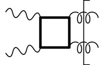
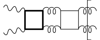
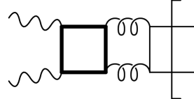
(a)	(b)	(c)
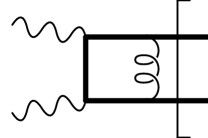
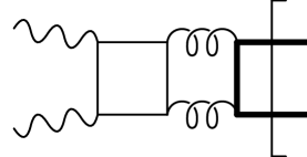
(d)	(e)	(f)

Figure 11: Diagrams with the $Z_{1}$ operation applied at the vertical line. The heavy quarks are denoted by the thick solid lines.

In the first three graphs, which have either gluons or light partons as their external lines, only the light quarks have their masses set to zero. But in the last three graphs, which have heavy quark external lines, all the quark masses should be set to zero; the external quarks will also be given massless on-shell momenta, $k^{2}=0$, and the Dirac matrix will be that for a massless quark.

If it is indeed valid to define $Z_{1}$ in this way, a substantial simplification is achieved in practical calculations, since it is only necessary to retain non-zero masses for heavy quarks in loops of heavy quark lines in coefficient functions with external light lines, i.e., in graphs such as the first three of Fig. 11.

The formal proof is as follows.

1. $H\cdot Z_{1}$ is only used when $H$ has a zero mass limit. Hence the virtualities in $H$ are of order $Q^{2}$ or larger. This is simply the assertion that collinear subtractions have been applied inside $H$, as in Eq. (85).

2. If $H$ and $T$ are joined by heavy quark lines, the virtuality of the heavy quark is at least of order $M^{2}$ in the dominant region of integration, for the whole leading power. The virtuality, as is well known, is in fact space-like.

3. In a region where the virtualities in $T$ are much less than the virtualities in $H$, then $H\cdot Z_{1}\cdot T$ provides as good an approximation to $H\cdot T$ as does the approximation with the heavy quark mass left non-zero. The original approximation involved replacing a momentum of space-like virtuality of order $M^{2}$ by an on-shell momentum. Instead we now replace it by a light-like momentum. The new $Z$ operation provides a suitable approximation given that the old operation did. Thus the first essential property of a $Z$ operation is obeyed

4. If the virtuality of the lines joining $H$ and $T$ is of order the virtualities in $H$, then setting masses to zero in $H$ changes the precise value but not the order of magnitude. Thus $H\cdot Z_{1}\cdot T$ is of the same magnitude as $H\cdot T$ in this case. The second property for $Z$ is satisfied.

5. The effect of $Z_{1}$ on $T$, in $Z_{1}\cdot T$, is the same as for $Z$. Thus there is no change in the logarithmic UV divergences that are generated.

A more physical argument can be made with the aid of an example. Consider the lowest order calculation of a heavy quark loop to a structure function. In Fig. 12, we have the Born graph for DIS on a heavy quark that comes out of the shaded target bubble. If $Q$ is much larger than the quark mass $M$, it is a useful approximation to replace the graph by the lowest order Wilson coefficient times the heavy quark density, as shown on the right of Fig. 12, for the important region when the quark has transverse momentum much less than $Q$. It is also a good approximation to replace $M$ by zero in the contribution to the coefficient function.

$$\hbox{\epsfbox{ht.eps}}\lower-1.29167pt~{}~{}~{}\longrightarrow~{}~{}~{}\hbox{\epsfbox{ht-approx.eps}}\lower-1.29167pt$$

Figure 12: Born graph for heavy quark in DIS.

$$~{}~{}~{}\longrightarrow~{}~{}~{} ~{}\left[~{}\hbox{\epsfbox{h1g1.eps}}\lower-1.29167pt~{}~{}-~{}~{}\hbox{\epsfbox{h1g2.eps}}\lower-1.29167pt~{}\right]\hbox{\epsfbox{gt.eps}}\lower-1.29167pt$$

$$+~{}~{}\hbox{\epsfbox{h1t1.eps}}\lower-1.29167pt$$

Figure 13: One-loop graph for heavy quark in DIS.

Now both of these approximations fail when $Q$ is comparable to $M$ (the “threshold region”). But in this case the heavy quark distribution is of order $\alpha_{s}$ relative to the gluon distribution. So to do valid phenomenology we must include also a one-loop coefficient times the gluon density. The result is shown in Fig. 13. We start with a particular kind of graph for the structure function where a heavy-quark loop couples to the target by gluon lines. To avoid extra irrelevant complications, suppose that the gluons have low virtuality. The first part of the right-hand side is a contribution to the coefficient function times the gluon density. In the one-loop coefficient there is a subtraction term. The second term on the right is the previously defined heavy quark coefficient function times a heavy quark density. In the region where the gluons have low virtuality this second term cancels the subtraction in the one-loop Wilson coefficient times the gluon density.

Hence the incorrectness in the approximation used in Fig. 12 is compensated by the subtraction in Fig. 13. Of course, it would have been much simpler to use the heavy quark (or “fixed-flavor”) scheme that we will discuss in Sec. X. But that scheme does not permit us to go to large $Q$, because there will then be large logarithms of $Q/M$ in its coefficient functions. In contrast, the scheme in Figs. 12 and 13 permits an interpolation between low and high $Q$ without loss of accuracy.

At sufficiently large $Q$, the Born term alone provides useful phenomenology, because the heavy quark density is large. Moreover, zero-mass coefficient functions can be used.

As $Q$ is decreased towards the threshold region, the Born term in the coefficient function becomes increasingly inaccurate as a representation of the graph on the left of Fig. 12. Note that even if we evaluate the coefficient with the correct mass there is still an error of the same order of magnitude as the error in neglecting the mass completely. This is because the horizontal lines are necessarily space-like. Replacing them with on-shell lines gives an error of order $M^{2}/Q^{2}$.

When one decreases $Q$, the errors in the approximation of Fig. 12 increase. At order $\alpha_{s}$, the errors are compensated by the subtraction term in Fig. 13. But beyond some point, the errors in the approximation become larger than the quantity one is trying to compute. Correct compensation of errors will involve the use of even higher order diagrams. Then one must abandon this scheme and use only the heavy quark scheme of Sec. X. The important point is that there is an overlap in the region of validity of both schemes.

X Factorization with $Q\lesssim M$

When $Q$ is reduced below the mass $M$ of a heavy quark, the scheme described in Sec. V becomes inappropriate. Indeed, given a fixed value of $x$, we go below the threshold at $Q=2M\sqrt{x/(1-x)}$ for producing the heavy quark by reducing $Q$ enough. On the other hand the factorization theorem that we derived earlier has a non-zero subprocess in which there is production of heavy quarks in the final state, for any value of $Q$. An example is given by Fig. 12. There we replace a graph for heavy quark production by the lowest order approximation to the factorization theorem. The replacement of an off-shell heavy quark by an on-shell quark in the hard scattering enables the approximated graph to be non-zero, even when the true physical process is below the threshold for producing heavy quarks. The error in the approximation is repaired by higher-order approximations to the coefficient functions, as illustrated in Fig. 13.

Clearly it is likely to be a poor and inaccurate method of calculation to obtain an answer that is known to be zero by adding a collection of non-zero pieces, in a truncated perturbation expansion. Even a little above threshold we may have inaccurate calculations: a cross section that approaches zero as the threshold is approached is calculated as a sum over terms that do not have the correct threshold behavior.

The remedy is to use a different version of the factorization theorem, in fact the well-known fixed-flavor-number scheme F2c ; DEN . In this section we present a proof of factorization in this scheme in a form that will mesh with the formulation and proof of factorization that we gave earlier. Using the terminology introduced in Sec. III, we will say that the heavy quark is treated as non-partonic. It will be convenient, for the purposes of this section, to call this scheme the “heavy-quark scheme”. The essence will be to treat the heavy quark as always being part of the hard scattering. This scheme has a range of validity that includes the whole region that $Q\lesssim M$. This range overlaps with the range of validity of the factorization theorem where the heavy quark is treated as partonic, i.e., the range $Q\gtrsim M$.

There are two important observations. One is that when $Q$ is of order $M$, the heavy quark mass provides a large scale of virtuality that can be treated on the same footing as $Q$. The second observation is that when $Q$ is much less than $M$, the decoupling theorem AC applies. Our heavy quark scheme will satisfy the decoupling theorem in the simplest way: one can simply drop all graphs involving heavy quark lines and obtain a correct answer without needed extra finite renormalizations of the coupling and parton densities. The method we will use is that of Collins, Wilczek and Zee CWZ , with the heavy quark begin treated as non-partonic. In that subscheme, renormalization is done in the $\overline{{\rm MS}}$ scheme for all graphs except those involving the heavy quark. For graphs with a heavy quark loop, renormalization is done by subtraction at zero momentum and with the light quark masses set to zero. The remaining renormalizations involve graphs with external heavy quark lines. Following Buza et al. BMSvN , we define the heavy quark mass as the position of the pole in the heavy quark propagator, a definition that makes sense in perturbation theory. Remaining renormalizations are defined by pole-part subtractions, in the $\overline{{\rm MS}}$ style.

This advantages of this scheme are CWZ :

1. It satisfies manifest decoupling.

2. $\overline{{\rm MS}}$ and zero momentum subtraction allow preservation of Ward identities in gauge theories without the need for extra finite counterterms.

3. Anomalous dimensions for the active partons and the $\beta$ function are the same as in the $\overline{{\rm MS}}$ scheme for the theory with the heavy quark omitted. They have no mass dependence.

4. At no stage, in either this subscheme or the subscheme where the heavy quark is active (or partonic), do we have to make an expansion in powers of $M/Q$ or $Q/M$: the heavy quark mass need never be approximated. So the scheme can be applied when there are several heavy quarks and the ratios of their masses are not necessarily large. Furthermore, there is no loss of accuracy when treating problems where a heavy quark is not heavy enough for it to decouple to high accuracy and not light enough for its mass to be approximated by zero.

In this section we will treat the case that the theory contains one heavy quark and that $Q\gtrsim M$. The most general case, that there are several heavy quarks, whose masses may or may not be larger than $Q$, will form an elementary generalization to be treated in Sec. XI. We will first derive a factorization theorem without taking account of renormalization and then we will do the renormalization.

X.1 Bare factorization theorem

When we are in the region $Q\lesssim M$, the leading regions continue to be of the form of Fig. 1. However, the specification of the graphs is a bit different, since heavy quark loops must each be contained in the hard part $H$ or in renormalization subgraphs of $T$. Thus the lines joining $H$ and $T$ must always be light partons. To obtain a factorization theorem, we use the reasoning in Sec. V with two changes.

The first change is that since heavy quarks cannot join the hard and target subgraphs, we change Eq. (17) so that the amplitudes corresponding to $C_{0}$, $K_{0}$, $T_{0}$ and $D$ are two-particle irreducible in the light partons only. The second change is that we need to take account of the decoupling theorem for graphs with heavy quark loops.

The first change means that Eq. (17) needs to be replaced by

$$F = \sum_{n=0}^{\infty}C_{H}\cdot(K_{H})^{n}\cdot T_{H}+D_{H}$$ (87)

$$= C_{H}\cdot\frac{1}{1-K_{H}}\cdot T_{H}+D_{H},$$

where the subscript $H$ means that the amplitude with the subscript is 2PI only in light parton lines. We can formalize the definitions of $C_{H}$, etc. by defining a projection $P_{L}$ that is unity on light lines and zero on heavy quark lines. The projector onto heavy lines is $P_{H}=1-P_{L}$. Then

$$C_{H} = C_{0}\cdot\frac{1}{1-P_{H}K_{0}}\cdot P_{L},$$

$$K_{H} = P_{L}\cdot K_{0}\cdot\frac{1}{1-P_{H}K_{0}}\cdot P_{L}=P_{L}\cdot\frac{1}{1-K_{0}P_{H}}\cdot K_{0}\cdot P_{L},$$

$$T_{H} = P_{L}\cdot\frac{1}{1-K_{0}P_{H}}\cdot T_{0},$$

$$D_{H} = D_{0}+C_{0}\cdot\frac{1}{1-P_{H}K_{0}}\cdot P_{H}\cdot T_{0}.$$ (88)

It can be verified that with these definitions, the structure function given by Eq. (87) is the same as before, i.e., $C_{0}\cdot\frac{1}{1-K_{0}}\cdot T_{0}+D_{0}$.

We define the remainder to be

$$r_{H}=C_{H}\cdot\frac{1}{1-(1-Z)K_{H}}\cdot(1-Z)\cdot T_{H}+D_{H}.$$ (89)

This remainder is power suppressed, just like the remainder $r$ that we defined in Eq. (18).

No changes are needed in the reasoning that lead to the bare factorization theorem Eq. (25). We find that

$$F=C_{HB}\otimes A_{B}+\mbox{non-leading power},$$ (90)

where the bare coefficient function is

$$C_{HB} = C_{H}\cdot\frac{1}{1-(1-Z)K_{H}}\cdot Z,$$ (91)

$$= C_{H}\cdot\frac{1}{1-(1-Z)K_{H}}\cdot Z\cdot P_{L},$$

and the bare operator matrix element (or bare parton density) is

$$P_{L}\cdot A_{HB} = P_{L}\cdot Z\cdot\frac{1}{1-K_{H}}\cdot T_{H}.$$ (92)

The leading regions only have active, light partons joining the hard subgraph and the target subgraph. This is reflected in the formulas by the fact that there are explicit factors of $P_{L}$ on the right of $C_{H}$, on the left of $T_{H}$ and on both sides of $K_{H}$. Hence we may insert the explicit factors of $P_{L}$ in the formulas for the coefficient function and operator matrix elements, Eqs. (91) and (92).

The reader should clearly understand the distinction between the following notations: $C_{0}$ is a fully 2PI and amputated Green function for two virtual photons and two quarks; $C_{H}$ is the same Green function as $C_{0}$ except for being 2PI only in light parton lines; and finally $C_{HB}$ is a Wilson coefficient: it is the full amputated Green function, including reducible graphs but with subtractions to make it a purely UV object.

Contrary to appearances, the definition Eq. (92) is equivalent to the previous definition, Eq. (24), so that

$$P_{L}\cdot A_{HB} = P_{L}\cdot Z\cdot\frac{1}{1-K_{0}}\cdot T_{0}{}.$$ (93)

The algebraic proof of this equation, starting from Eq. (92), is left as an exercise. We can also define the densities of heavy quarks by $P_{H}\cdot A_{HB}=P_{H}\cdot Z\cdot\frac{1}{1-K_{0}}\cdot T_{0}$, but we will not need to use the definition here, since only light parton densities appear in the factorization theorem.

At first sight it appears that the bare parton densities $A_{HB}$ are identical to those in the previous version of the factorization theorem. This is not quite so, because we are using a different renormalization subscheme for the QCD action, both subschemes being part of the CWZ CWZ family of schemes. Green functions in the two subschemes differ by factors associated with the changes in the wave function renormalization factors. In addition, even without wave function renormalization, the numerical values of the coefficients in the perturbation expansion of $K_{0}$, etc., would differ because the numerical value of the coupling $\alpha_{s}$ differs between the two subschemes. This can all be summarized by saying that $K_{0}$, $T_{0}$ and $C_{0}$ in the two subschemes differ by a renormalization group transformation.

When we renormalize the operators, and hence construct the renormalized factorization theorem, we will need to work in terms of $K_{0}$ rather than $K_{H}$. So we rewrite our new coefficient function $C_{HB}$ in terms of fully 2PI amplitudes. This is done quite simply by defining a new projection operator $Z_{H}$ that is zero when applied to heavy quark lines and that is $Z$ on light parton lines. Then $Z_{H}=Z\cdot P_{L}$.

Graphically, the coefficient function $C_{HB}$ given in Eq. (91) is $C_{0}$ with any number of $K_{0}$’s attached. If neighboring rungs are connected by active partons, then a factor of $1-Z$ is inserted, but connections by heavy quarks are left unaltered. A straightforward but somewhat lengthy algebraic derivation shows that Eq. (91) implies that

$$C_{HB}=C_{0}\cdot\frac{1}{1-(1-Z_{H})K_{0}}\cdot Z\cdot P_{L}.$$ (94)

Observe that on an active light parton $1-Z_{H}=1-Z$ and on a heavy quark $1-Z_{H}=1$, so that this equation agrees with the verbal description given at the beginning of the paragraph.

X.2 Renormalized factorization theorem

Next we copy and slightly modify the steps needed to derive the renormalized factorization theorem. To define the renormalized parton densities, we need to use a renormalization scheme in which the heavy parton is treated as non-partonic. So we define

$$A_{HR} = \sum_{n=0}^{\infty}Z\cdot\left[K_{0}\cdot\left(1-\loarrow{\cal P}_{H}\right)\right]^{n}\cdot T_{0}$$ (95)

$$= Z\cdot\frac{1}{1-K_{0}\cdot\left(1-\loarrow{\cal P}_{H}\right)}\cdot T_{0}.$$

The renormalization is defined by $\loarrow{\cal P}_{H}$, which is an operation that acts to the left. We define $L\loarrow{\cal P}_{H}$ as follows: If $L$ contains heavy quark loops and its rightmost external lines are light partons, then $L\loarrow{\cal P}_{H}$ is the value of $L(q,k,M,m)$ when $k^{-}$ and ${\bf k}_{T}$ are replaced by zero and the light parton masses $m$ are replaced by zero. If $L$ contains no heavy lines, then, $L\loarrow{\cal P}_{H}$ is just the $\overline{{\rm MS}}$ pole part of $L$. The remaining case is when we apply $\loarrow{\cal P}_{H}$ to graphs with external heavy lines. There is a choice of scheme that is not determined by the overall requirements listed in Sec. II. This is similar to the non-uniqueness found by Roberts and Thorne RT2 ; RT1 . We will choose to define the operation to be pole-part subtraction, in the $\overline{{\rm MS}}$ style, as we did in a similar situation when renormalizing the interactions.

In accordance with the dictates of the BPH approach to renormalization, counterterms are kept with the graphs they subtract. Thus $L\loarrow{\cal P}_{H}$ is only used when $L$ is a quantity for which all subdivergences have been subtracted. This also ensures CWZ that the use of zero momentum subtractions for subgraphs containing heavy quark loops introduces no IR divergences in the counterterms.

With these definitions, we can copy most of the previous derivation of a renormalized factorization theorem. First we observe the the relation between renormalized and bare parton densities has the form

$$A_{HR}=G_{H}\otimes A_{HB},$$ (96)

where we use

$$G_{H}\equiv Z-Z\cdot\frac{1}{1-K_{0}\cdot\left(1-\loarrow{\cal P}_{H}\right)}\cdot K_{0}\loarrow{\cal P}$$ (97)

instead of $G$ given by Eq. (59). Then we express the factorization theorem in terms of renormalized parton densities

$$F=C_{HR}\otimes A_{HR}+\mbox{remainder, $r_{H}$},$$ (98)

where the renormalized coefficient function is

$$C_{HR}=C_{HB}\otimes G_{H}^{-1}.$$ (99)

Finally, we bring in the decoupling theorem. This implies that a renormalized graph for $A_{HR}$ is suppressed by a power of $\Lambda/M$ if it contains any heavy quark lines. This is a consequence of the use of a renormalization scheme which obeys manifest decoupling, for both the interaction and operator matrix elements. We are assuming here that the target hadron in the structure function is a light hadron. One case of this result is that the density of a heavy quark is power suppressed in the scheme we are using in this section. This result only applies to the renormalized heavy quark density, not to the bare heavy quark density.

We can therefore restrict the renormalized coefficient function so that its external lines are light, and the factorization theorem becomes

$$F=C_{HR}\otimes A_{LR}+\mbox{power-suppressed remainder},$$ (100)

where now the parton densities $A_{LR}$ are renormalized parton densities in the effective low energy theory with the heavy quark omitted. There appears to be no simple formula for the remainder, and notice that the remainder is not equal to $r_{H}$ defined in Eq. (89).

As before, there appears to be no simple formula for the coefficient function, but a simple recursion formula does exist and it corresponds to the algorithms actually used to do calculations. The formula is almost the same as the previous one, Eq. (74):

$$C_{HR}^{(n)}=F_{p}^{(n)}-\sum_{j=0}^{n-1}C_{HR}^{(j)}A_{LRp}^{(n-j)}.$$ (101)

The structure function is to be computed on a light-parton target only, not on a heavy target, and the light-parton masses are to be set to zero. The parton density has subscripts $LRp$, whose meaning is as follows: The $L$ indicates that $A_{LRp}$ is computed with the omission of all graphs containing heavy-quark lines. The $R$ indicates that it is renormalized, and the $p$ indicates the same (zero-mass light-parton) target as for the structure function.

The one complication in proving Eq. (101) results from the fact that in deriving the factorization theorem, Eq. (100) on a general target, we omitted graphs for $A_{LR}$ that contain heavy lines, but without giving a formula for the omitted terms. So the recursion formula Eq. (101) could be in error by similar terms, i.e., there might be a power-suppressed remainder term on the right-hand side. In fact all graphs for $A_{LRp}$ that include heavy quark lines are exactly zero when combined with their counterterms. This is because they are being evaluated with their external momenta at exactly the subtraction point. Hence Eq. (101) is exact.

X.3 Differences between heavy and light factorization

The renormalized factorization theorem with heavy quarks, Eq. (100), differs from the first factorization theorem Eq. (62) in two respects:

1. The sum over partons in the heavy quark factorization is restricted to light partons only.

2. The parton densities differ by a change of scheme.

The first point accounts for our terminology of contrasting “active” (or “partonic”) with “non-partonic” quarks. In the factorization we derived for $Q\gtrsim M$, Eq. (62), the heavy quark is partonic: there is a term involving hard scattering off a heavy quark. In contrast, in the factorization for $Q\lesssim M$, Eq. (100), there is no such term.

There is an overlapping domain of utility of the two schemes. This is where both $Q$ and the $\overline{{\rm MS}}$ scale $\mu$ are of order $M$. In this situation there are no large logarithms in the coefficient functions and no large logarithms in the coefficients that relate the two schemes. This overlap is important because it implies that the relation between the parton densities in the two schemes can be computed perturbatively. In practical applications it should be remembered that at large $x$, the physical threshold for heavy-quark production can be well above $Q$, and consequently the region where the two schemes have common domains of utility should then be appropriately biased upwards in $Q$.

When the heavy quark is treated as non-partonic, its parton density is not used in the factorization theorem, and one might suppose that the heavy quark density does not exist at all. In fact the heavy quark density does exist, because one can define it by exactly the usual operator formula, together with renormalization (as dictated by the CWZ scheme). The important fact is that the heavy quark (and antiquark) densities can be expressed in terms of the light parton densities by a version of factorization. This is a heavy quark expansion for matrix elements of heavy-quark operators in light states, and the argument was first given by Witten Witten for the case of local operators. In the subscheme where the heavy quark is non-partonic, the result is quite simple: the heavy quark densities are suppressed by a power of the heavy quark mass:

$$f_{H/p}=O(\Lambda/M).$$ (102)

We used this property in our derivation of the factorization theorem.

XI Multiple heavy quarks

Let us now suppose that we have the most general case that there are several heavy quarks, whose masses may or may not differ greatly, and that $Q$ can vary over a wide range.

XI.1 Factorization

In this situation, we define a series of subschemes, each of which is labeled by the subset of the flavors of quarks and gluon which are treated as active (or partonic). The other flavors in the subscheme we call non-partonic. The choice of subscheme is made according to the value of $Q$. If $Q$ is much larger than the mass of a particular quark, then that quark is partonic. If $Q$ is much smaller than the mass of a particular quark, then that quark is non-partonic. If $Q$ is comparable to the mass of a particular quark, we may freely choose whether the quark is partonic or non-partonic. Gluons are light, so they are always partonic. We can define the scheme by saying that the $n_{A}$ lightest quarks are partonic.

Factorization is derived by a minor extension of the procedure in Sec. X. In that section we had one heavy quark, which was treated as non-partonic, with the gluon and other quarks being treated as partonic. We simply need to replace all references to a “heavy quark” by references to “non-partonic quarks”. Thus renormalization counterterms are generated by $\overline{{\rm MS}}$ pole terms, except for mass renormalization of heavy quarks, which is always performed on shell, and except for graphs with loops of non-partonic quarks, whose counterterms are computed at zero external momentum and with the masses of the active partons set to zero. This defines the appropriate version of the renormalization operator that is to replace $\loarrow{\cal P}$ in Eq. (56) or $\loarrow{\cal P}_{H}$ in Eq. (95).

In the construction of the coefficient function and the remainder for the factorization formula, the operation $Z_{H}$ must be replaced by $Z_{n_{A}}$, which is $Z$ when applied on an active quark or gluon and zero on non-partonic quarks.

The methods used to construct the two factorization proofs readily generalize to show that the remainder is suppressed by a power of $Q$, provided that all the active partons have masses less than or of the order of $Q$. Moreover, in the perturbative expansion of the coefficient function, if the $\overline{{\rm MS}}$ scale $\mu$ is of order $Q$, there will be no large logarithms of ratios of $Q$, $\mu$ and quark masses provided also that the masses of the non-partonic quarks are all larger or comparable with $Q$. The coefficient functions have infra-red-safe limits when masses of active partons are set to zero. (This applies in particular to the light quarks; their masses may always be set to zero in the coefficient functions.)

XI.2 When can the masses of active partons be set to zero?

The setting to zero of active parton masses in the renormalization prescription is necessary to get the simplest results, for example for the renormalization-group coefficients. It is always legitimate.

Moreover, if one is computing the coefficient function for a particular external quark, then one can set to zero the mass of this quark and of the lighter partons, as explained around Eq. (86). It is only with this prescription that the recursion formula for the coefficient function, Eq. (101) is exact.

As an example, suppose that one is treating the charm quark (of mass $m_{c}=1.5\,{\rm GeV}$) as partonic but the bottom quark (of mass $m_{b}=4.5\,{\rm GeV}$) as non-partonic. This implies that we are treating phenomena on a scale of at least $m_{c}$. Furthermore, suppose that one has decided that the charm quark is not sufficiently light compared to $m_{b}$ for its mass to be neglected. Then in coefficient functions with external gluons, for example, one leaves both the masses of the charm and bottom quarks at their physical values. In contrast, in a coefficient function with an external charm quark, its mass may be set to zero. As explained around Eq. (86), this may be done without loss of accuracy, since any errors are taken care of by higher-order coefficients with lighter external partons.

XII Matching conditions and evolution equations

XII.1 Matching conditions

As a consequence of the decoupling theorem, the density of a non-partonic quark is suppressed by a power of $\Lambda/M$, where $M$ is the mass of the quark, so we will normally approximate these densities by zero.

Furthermore there are matching conditions between the parton densities with $n_{A}$ and $n_{A}+1$ active quarks. The coefficients relating the parton densities are functions of the quark masses and $\mu$, and have no large logarithms provided that $\mu$ is of the order of the mass of quark $n_{A}+1$. The coefficients also have infra-red-safe limits when the masses of the $n_{A}$ lightest quarks are set to zero.

These matching conditions, have been given in Ref. ACOT to order $\alpha_{s}$ and in Ref. BMSvN to order $\alpha_{s}^{2}$. They are applied to calculate the parton densities with $n_{A}+1$ active quarks from the parton densities with $n_{A}$ active quarks. The conditions are to be applied at a value of the renormalization scale around the mass of quark $n_{A}+1$. Given that we set the density of the quark $n_{A}+1$ to zero when it is non-partonic, the matching conditions give initial values for all $n_{A}+1$ quarks and the gluon which can therefore be evolved upward in scale. This gives an effective calculation of the density of quark $n_{A}+1$ in the region where it is active.

XII.2 Evolution equations

We have a series of schemes labeled by the number of active quarks, $n_{A}=3,4,5,\dots$. In each scheme we have densities for the gluon and for each of the active quarks and antiquarks. Up to power-suppressed corrections, the densities of the non-partonic quarks and antiquarks are zero. The active partons evolve according to the standard DGLAP evolution equations, with the kernels being those of the $\overline{{\rm MS}}$ with $n_{A}$ flavors.

XIII Miscellaneous comments

XIII.1 Relation to other methods of treating heavy quarks

Calculations of heavy quark production often use what is called a fixed-flavor-number scheme F2c ; photo ; DEN ; had.heavy . This corresponds exactly to the method described in the present paper if the heavy quark is treated as non-partonic. (For example, it corresponds to a 3-flavor scheme for charm production and to a 4-flavor scheme for bottom production.)

Other calculations switch between different numbers of active quarks, but neglect the masses of the active quarks in the coefficient functions. This is a valid approximation to the scheme here when power corrections in $M/Q$ are negligible, but not when these power corrections are important. The scheme described in this paper does not require the masses of active quarks to be neglected.

I have been unable to discover the justification of the scheme proposed by Martin, Roberts, Ryskin and Stirling MRRS .

Roberts and Thorne RT2 ; RT1 appear to have a scheme similar to the one in the present paper. But they do not present complete proofs, and they make a number of incorrect or misleading statements. For example, they state that “the detailed construction of the coefficient functions …is extremely difficult if not impossible.” As regards the general formalism, the construction is exactly as difficult as in the light-quark case. The only computational complication is that in a calculation of the coefficient functions, heavy quark masses must be retained. All the necessary Feynman-graph calculations for computing the coefficient functions at order $\alpha_{s}^{2}$ have been done in Refs. BMSvN , and all that remains is to organize them to form the coefficient function by use of the recursion relation Eq. (74). This recursion relation is of the same form as the one used to obtain the coefficient functions in the massless case.

XIII.2 Modification of the schemes

It is possible to redefine the factorization results by a change of scheme that defines the parton densities. This is in effect a change of the renormalization operation that defines them.

In addition, the details of the extraction of the asymptotics of the structure functions may be changed by redefining the $Z$ operation. The constraints on allowed redefinitions were explained in Sec. IX.4, and they are implied by the requirements for a good factorization scheme that were listed in Sec. II. The $Z$ operations and the renormalization operation should not change the validity of the error estimates used in the proof of factorization.

I consider the $\overline{{\rm MS}}$ scheme to be the best underlying scheme at the present state of the art, since it is the scheme most commonly used for calculations of QCD corrections to hard processes (at least when masses are ignored).

XIII.3 Comparison with Zimmermann’s approach

One often gets the impression that Zimmermann’s derivation Zimmermann of the operator product expansion (OPE) is considered as the most reliable. However, Zimmermann does not in fact prove the results that we need for regular QCD phenomenology, even if we restrict to the case that the OPE is sufficient. (The derivation in the present paper in fact applies to the Minkowski space structure functions, rather than only to the integer moments of the structure functions. It is to these integer moments that the OPE in its strict sense is restricted.)

His results suffer from two disadvantages. The first is that his Wilson coefficients have divergences in the zero-mass limit. They are not infra-red safe, and further work is needed to put the results in a useful form for perturbative phenomenology in QCD. The second disadvantage is that his evolution equations are the inhomogeneous Callan–Symanzik equations rather than the homogeneous renormalization-group equations that can actually be used in practice. The inhomogeneous term is not of a form susceptible to easy calculation, so further work is needed to show that to a suitable approximation, this term can be neglected. In Tkachov’s terminology perfect , Zimmermann’s version of the OPE does not give a “perfect asymptotic expansion” at large $Q$. In contrast, the factorization proved in the present paper is perfect in this sense.

In this section, we will see how Zimmermann’s results can be proved by our methods, and that they indeed suffer from the above mentioned disadvantages.

The algebraic steps that led to our factorization theorem are shown in Eq. (22). The strategy in organizing the manipulations was that the right-most factor of $Z$ should be made explicit. Zimmermann’s result can be obtained by arranging so that the left-most $Z$ is picked out. This results in the following derivation:

$$F-r = C_{0}\cdot\left[\frac{1}{1-K_{0}}-(1-Z)\frac{1}{1-K_{0}(1-Z)}\right]\cdot T_{0}$$ (103)

$$= C_{0}\cdot\frac{1}{1-K_{0}}\cdot\left[1-K_{0}(1-Z)-(1-K_{0})(1-Z)\right]\cdot\frac{1}{1-K_{0}(1-Z)}\cdot T_{0}$$

$$= C_{0}\cdot\frac{1}{1-K_{0}}\cdot Z\cdot\frac{1}{1-K_{0}(1-Z)}\cdot T_{0}.$$

We therefore have a factorization theorem

$$F=C_{Z}\otimes A_{Z}+\mbox{non-leading power},$$ (104)

where the coefficient function is

$$C_{Z}=C_{0}\frac{1}{1-K_{0}}Z,$$ (105)

and the operator matrix element is

$$A_{Z}=Z\frac{1}{1-K_{0}(1-Z)}T_{0}.$$ (106)

Notice first that the operator matrix element $A_{Z}$ in Zimmermann’s approach is already ultra-violet finite: the $1-Z$ factors in Eq. (106) provide the necessary counterterms. This is contrast with our approach in Sect. V, where some extra work was needed to express the factorization in terms of renormalized operators. Unfortunately, the counterterms in Zimmermann’s approach are calculated at zero momentum, and so they suffer from divergences in the massless limit, notably for the gluons. Thus although the bare matrix elements (without renormalization) are infra-red finite, if the hadron state is well behaved, the renormalization procedure introduces mass divergences.

Moreover the coefficient function is ultra-violet finite, since it is just a Green function of two currents and two partons. In Zimmermann’s work, on the OPE, the external partons of the coefficient function are given zero momentum; this corresponds to his use of zero momentum subtractions to do renormalization. The correct generalization to Minkowski space problems is given by the operator $Z$ defined in Eq. (8): only the “$-$” and transverse components of a momentum are set to zero. Our derivation works equally well with on-shell renormalization, with $Z$ defined by Eq. (11).

However, Zimmermann’s definition of the coefficient is not infra-red finite. One cannot set the masses to zero. This is the strongest reason for not regarding Zimmermann’s approach as adequate for the problems we are interested in. It is a particular problem in QCD as opposed to other field theories, since the gluon is intrinsically massless.

XIII.4 Other processes

Exactly the same methods that have been explained here can be applied to other processes. Also, if there turn out to be other fields with color interactions, for example, squarks or gluinos, they can be treated by minor generalizations of the same methods: we have the choice of treating each massive field as either partonic or non-partonic.

XIV Conclusions

I have given a proof of factorization for deep-inelastic structure functions including the effects of heavy quarks. The methods are general and include all non-leading logarithms. The scheme implemented is exactly that of ACOT ACOT . The proof is applicable independently of the relative sizes of the heavy quark masses and $Q$, and the size of the errors is a power of $\Lambda/Q$. It can be readily extended to other hard processes.

Although this paper is quite lengthy, its core is really quite short. The essential elements of the proof are:

1. Power counting is used to prove that the leading regions have the form symbolized by Fig. 1. This is a standard basic result of perturbative QCD.

2. The remainder, as defined in Eq. (18), is then proved to be a non-leading power. The proof is fairly obvious given the form of the leading regions.

3. The bare form of factorization then follows from the three lines of algebra given in Eq. (22).

4. Renormalization of the parton densities is implemented in Eq. (56). Then applying the inverse renormalization factor gives the renormalized factorization theorem.

5. Application of the factorization theorem to a parton target gives an algorithm for computing the coefficient function.

This gives the factorization theorem when a heavy quark is treated as partonic. Simple modifications, plus the use of the decoupling theorem, give the corresponding results when a heavy quark is non-partonic.

When one is treating a heavy quark as partonic, it is valid to include the heavy quark in the sum over partons in the factorization formula even though it cannot really be treated as a parton, in Feynman’s sense. Errors in doing this are automatically taken care of by the inclusion of higher-order terms in the coefficient functions. Since the heavy quark densities and the light parton densities are of different sizes in the threshold region, a correct leading-order calculation can only be done if lowest-order coefficient functions are included for all possible subprocesses. The lowest-order coefficient functions are of different orders in $\alpha_{s}$: The quark-induced processes have a lowest order $1$, and the gluon induced process has a lowest order $\alpha_{s}$. As $Q$ changes, the relative contributions of the different subprocesses change in size. This mixing of orders is to be expected in any problem where the parton densities have very different sizes, and is not incorrect, contrary to the assertion of Roberts and Thorne RT1 .

Notice that there is an implicit unitarity sum over final states in the whole of our work. As explained on page 2, this implies that the details of the final-state interactions do not affect factorization or the calculation of the coefficient functions. In particular, it is irrelevant that in Feynman-graph calculations, there are on-shell partons in the final-state, even though in the real-world there are only physical hadrons in the final-state.

Misleading derivation of formula for renormalized coefficient function

In this appendix we show some apparently correct manipulations can be used to justify a plausible but wrong formula for the renormalized coefficient function. The formula is

$$C_{\rm cand}=C_{0}\cdot\frac{1}{1-(1-Z)\cdot K_{0}}\cdot(1-\loarrow{\cal P})\cdot Z.$$ (107)

(The subscript “cand” is to indicate this is a candidate for the renormalized coefficient function.) Expanded in powers of $K_{0}$ this gives

$$C_{\rm cand}=C_{0}\cdot\sum_{n=0}^{\infty}[(1-Z)K_{0}]^{n}\cdot(1-\loarrow{\cal P})\cdot Z.$$ (108)

This candidate coefficient function has some properties that make it an obvious candidate for a renormalized coefficient function:

1. The factors of $1-Z$ prevent there from being leading contributions from regions where the momenta on the left are much higher in virtuality than those on the right.

2. This includes the case that the left-hand momenta are hard momenta, of virtuality of order $Q^{2}$, as in the leading regions Fig. 1, as well as the momenta that give ultra-violet divergences.

3. Thus the only leading regions are where all the momenta in $C_{\rm cand}$ are of virtuality of order $Q^{2}$ or where there is an ultra-violet divergence where all the momenta in some right-hand part of $C_{\rm cand}$ go to infinity.

4. The factor $1-\loarrow{\cal P}$ cancels all the ultra-violet divergences.

5. The right-most factor of $Z$ defines the standard approximation appropriate to defining a hard-scattering coefficient that is coupled to a collinear target factor.

Therefore $C_{\rm cand}$ represents an obvious way of applying ultra-violet renormalization to the bare coefficient function defined in Eq. (23).

Let us now attempt to prove the factorization formula

$$F=C_{\rm cand}\otimes A_{R}+\mbox{non-leading power}.$$ (109)

The following manipulations use just ordinary linear algebra, together with the definitions of $C_{B}$, $A_{B}$, and $A_{R}$, and the properties $Z^{2}=Z$ and $\loarrow{\cal P}Z=\loarrow{\cal P}$:

$$C_{\rm cand}\otimes A_{R} = C_{0}\frac{1}{1-(1-Z)K_{0}}(1-\loarrow{\cal P})ZG\otimes A_{B}$$ (110)

$$= C_{B}(Z-\loarrow{\cal P})\left[Z-ZK_{0}\frac{1}{1-(1-\loarrow{\cal P})K_{0}}\loarrow{\cal P}\right]A_{B}$$

$$= C_{B}\left[Z-\loarrow{\cal P}-(ZK_{0}-\loarrow{\cal P}K_{0})\frac{1}{1-(1-\loarrow{\cal P})K_{0}}\loarrow{\cal P}\right]A_{B}$$

$$= C_{B}\left[Z-\loarrow{\cal P}+(1-K_{0}+\loarrow{\cal P}K_{0}-1+K_{0}-ZK_{0})\frac{1}{1-(1-\loarrow{\cal P})K_{0}}\loarrow{\cal P}\right]A_{B}$$

$$= C_{B}\left[Z-(1-(1-Z)K_{0})\frac{1}{1-(1-\loarrow{\cal P})K_{0}}\loarrow{\cal P}\right]A_{B}$$

$$= C_{B}\otimes A_{B}-C_{0}\frac{1}{1-(1-\loarrow{\cal P})K_{0}}\loarrow{\cal P}A_{B}$$

$$= C_{B}\otimes A_{B}-C_{0}\frac{1}{1-K_{0}}\left(1-K_{0}\right)\frac{1}{1-(1-\loarrow{\cal P})K_{0}}\loarrow{\cal P}A_{B}$$

$$= C_{B}\otimes A_{B}-C_{0}\frac{1}{1-K_{0}}\left(1-(1-\loarrow{\cal P})K_{0}-\loarrow{\cal P}K_{0}\right)\frac{1}{1-(1-\loarrow{\cal P})K_{0}}\loarrow{\cal P}A_{B}$$

$$= C_{B}\otimes A_{B}-C_{0}\frac{1}{1-K_{0}}\loarrow{\cal P}\left[1-K_{0}\frac{1}{1-(1-\loarrow{\cal P})K_{0}}\loarrow{\cal P}\right]A_{B}.$$

In the second term of the extreme right-hand side, we have a pole-part operation applied to a quantity without ultra-violet divergences, $C_{0}/(1-K_{0})$. This second term is therefore zero, and we appear to have proved $C_{\rm cand}\otimes A_{R}=C_{B}\otimes A_{B}$, which is sufficient to prove factorization, since $C_{B}\otimes A_{B}$ equals the structure function $F$, up to a power-suppressed remainder.

Unfortunately, the above derivation is false. It has assumed that the operation of taking the pole part obeys all the rules of linear algebra, including associativity. The problem can be seen at the first order in $K_{0}$. There are two terms on the left-hand side of Eq. (110):

$$\left[C_{0}(1-Z)K_{0}(1-\loarrow{\cal P})Z\right]\left[ZT_{0}\right]+\left[C_{0}Z\right]\left[ZK_{0}(1-\loarrow{\cal P})T_{0}\right].$$ (111)

The square brackets are used to delimit factors belonging to the coefficient and to the operator. The terms with a pole-part are

$$-\left[C_{0}(1-Z)K_{0}\loarrow{\cal P}\right]\left[ZT_{0}\right]-\left[C_{0}Z\right]\left[ZK_{0}\loarrow{\cal P}T_{0}\right]=\left[C_{0}ZK_{0}\loarrow{\cal P}\right]\left[ZT_{0}\right]-\left[C_{0}Z\right]\left[ZK_{0}\loarrow{\cal P}T_{0}\right],$$ (112)

where we have observed (correctly) that $C_{0}K_{0}$ has no ultra-violet divergence.

The two terms in Eq. (112) appear to cancel. In fact this is not so. We are taking

$$\left[\mbox{pole part}(C_{0}ZK_{0})\right]T_{0}-C_{0}Z\left[\mbox{pole part}(ZK_{0})\right]T_{0}.$$ (113)

This is not, in general, zero, as can be seen by taking a simple mathematical example. Let us replace $C_{0}Z$ and $ZK_{0}$ by

$$C_{0}Z=1+a\epsilon,~{}~{}~{}ZK_{0}=\frac{1}{\epsilon}+b.$$ (114)

Then Eq. (113) becomes

$$\mbox{pole part}\left[(1+a\epsilon)\left(\frac{1}{\epsilon}+b\right)\right]-(1+a\epsilon)\mbox{pole part}\left(\frac{1}{\epsilon}+b\right) = \frac{1}{\epsilon}-(1+a\epsilon)\frac{1}{\epsilon}$$ (115)

$$= -a,$$

which is clearly non-zero.

Treating $\loarrow{\cal P}$ as an associative operator has failed.

References

- (1) E. Laenen, S. Riemersma, J. Smith, and W.L. van Neerven, Nucl. Phys. B392, 162 (1993); S. Riemersma, J. Smith, and W.L. van Neerven, Phys. Lett. B347, 143 (1995), hep-ph/9411431.
- (2) J. Smith and W.L. van Neerven, Nucl. Phys. B374, 36 (1992).
- (3) M. Glück, S. Kretzer, and E. Reya, Phys. Lett. B398, 381 (1997), Erratum-ibid. B405, 392 (1997), hep-ph/9701364; M. Glück, E. Reya, and M. Stratmann, Nucl. Phys. B422, 37 (1994).
- (4) P. Nason, S. Dawson, and R.K. Ellis, Nucl. Phys. B327, 49 (1989), Erratum—ibid. B335, 260 (1990), and Nucl. Phys. B303, 607 (1988).
- (5) W. Beenakker, W.L. van Neerven, R. Meng, G.A. Schuler, and J. Smith, Nucl. Phys. B351, 507 (1991); W. Beenakker, H. Kuijf, W.L. van Neerven, and J. Smith, Phys. Rev. D40, 54 (1989).
- (6) M.A.G. Aivazis, J.C. Collins, F.I. Olness, and W.-K. Tung, Phys. Rev. D50, 3102 (1994), hep-ph/9312319; J.C. Collins and W.-K. Tung, Nucl. Phys. B278, 934 (1986).
- (7) M. Cacciari. M. Greco, and P. Nason, hep-ph/9803400.
- (8) M. Buza, Y. Matiounine, J. Smith, and W.L. van Neerven, Eur. Phys. J. C1, 301 (1998), hep-ph/9612398; M. Buza, Y. Matiounine, J. Smith, R. Migneron, and W.L. van Neerven, Nucl. Phys. B472, 611 (1996), hep-ph/9601302.
- (9) A.D. Martin, R.G. Roberts, M.G. Ryskin, and W.J. Stirling, Eur. Phys. J. C2, 287 (1998), hep-ph/9612449.
- (10) R.S. Thorne and R.G. Roberts, Phys. Lett. B421, 303 (1998), hep-ph/9711223.
- (11) R.S. Thorne and R.G. Roberts, Phys. Rev. D57, 6871 (1998), hep-ph/9709442.
-
(12)
J. Collins, F. Wilczek, and A. Zee,
Phys. Rev. D18, 242 (1978);
J.C. Collins, Renormalization, (Cambridge University Press, Cambridge, 1984), ch. 8. - (13) Particle Data Group, R.M. Barnett et al., Review of Particle Physics, Phys. Rev. D54, 1 (1996).
- (14) K.G. Chetyrkin, B.A. Kniehl, and M. Steinhauser, Phys. Rev. Lett. 79, 2184 (1997), hep-ph/9706430; K.G. Chetyrkin, B.A. Kniehl, and M. Steinhauser, Nucl. Phys. B510, 61 (1998), hep-ph/9708255, and references therein.
- (15) See ACOT and the first reference of BMSvN for matching of parton distribution functions.
- (16) F.V. Tkachov, Phys. Lett. B124, 212 (1983).
- (17) T. Appelquist, and J. Carazzone, Phys. Rev. D11, 2856 (1975).
- (18) G. Curci, W. Furmanski, and R. Petronzio, Nucl. Phys. B175, 27 (1980).
- (19) R.K. Ellis, H. Georgi, M. Machacek, H.D. Politzer, and G.G. Ross, Nucl. Phys. B152, 285 (1979).
- (20) J.C. Collins, D.E. Soper, and G. Sterman, Nucl. Phys. B261, 104 (1985), and Nucl. Phys. B308, 833 (1988); G. Bodwin, Phys. Rev. D31, 2616 (1985), and D34, 3932 (1986).
- (21) S. Libby and G. Sterman, Phys. Rev. D18, 3252 and 4737 (1978).
- (22) K.G. Chetyrkin, F.V. Tkachov, and S.G. Gorishnii, Phys. Lett. 119B, 407 (1982).
- (23) F.V. Tkachov, Sov. J. Part. Nucl. 25, 649 (1994), hep-ph/9701272; F.V. Tkachov, Int. J. Mod. Phys. A8, 2047 (1993), hep-ph/9612284.
- (24) C.G. Callan, Phys. Rev. D2, 1541 (1970); K. Symanzik, Commun. Math. Phys. 18, 227 (1970).
- (25) E. Witten, Nucl. Phys. B104, 445 (1976).
- (26) For a pedagogical account, see G. Sterman, “Partons, Factorization and Resummation,” in “Theoretical Advanced Study Institute in Elementary Particle Physics, 1995: QCD and Beyond (TASI ’95),” D.E. Soper, ed. (World Scientific, Singapore, 1996).
- (27) P.V. Landshoff and J.C. Polkinghorne, Phys. Rept. 5, 1 (1972).
- (28) J.C. Collins and G. Sterman, Nucl. Phys. B185, 172 (1981).
-
(29)
A.V. Efremov and A.V. Radyushkin,
Teor. Mat. Fiz. 44, 327 (1980)
[Eng. transl.: Theor. Math. Phys. 44, 774 (1981)];
J.M.F. Labastida and G. Sterman, Nucl. Phys. B254, 425 (1985). - (30) J.C. Collins, Nucl. Phys. B394, 169 (1993), hep-ph/9207265.
- (31) J.C. Collins and D.E. Soper, Nucl. Phys. B194, 445 (1982).
- (32) R.P. Feynman, Photon-Hadron Interactions (Benjamin, 1972).
- (33) J.C. Collins, D.E. Soper, and G. Sterman, “Factorization of Hard Processes in QCD” in “Perturbative QCD” (A.H. Mueller, ed.) (World Scientific, Singapore, 1989). See p. 43.
-
(34)
V.A. Ilyin, M.S. Imashev and D.A. Slavnov, Teor. Mat. Fiz. 52, 177 (1982);
D.A. Slavnov, Teor. Mat. Fiz. 62, 335 (1985);
J.C. Collins, “Choosing the renormalization/factorization scale”, in Proceedings of the Jet Studies Workshop, Durham, U.K., December 9–15, 1990, J. Phys. G 17, 1549 (1991).
A.N. Kuznetsov and F.V. Tkachov, “Multiloop Feynman Diagrams and distribution theory, (III) UV renormalization in momentum space”, preprint NIKHEF-H/90-17. - (35) S.J. Brodsky, Y. Frishman, G.P. Lepage, and C. Sachrajda, Phys. Lett. 91B, 239 (1980).
- (36) W. Zimmermann, Ann. Phys. (N.Y.) 77, 570 (1973).