Perturbative QCD calculations with heavy quarks

Abstract

We review recent calculations of second order corrections to heavy quark decays. Techniques developed in this context are applicable to many processes involving heavy charged particles, for example the nonabelian dipole radiation. Calculations involving relativistic radiating particles are also discussed.

1 Introduction

Description of the higher order QCD effects in heavy quark processes is important in view of the improving experimental precision. Ongoing efforts to determine the CKM matrix elements motivate a thorough theoretical description of $B$ meson decays (for a review see [1]). These studies are made difficult by the complexity of the initial state, however even their conceptually simplest part — perturbative ${\cal O}(\alpha_{s}^{2})$ QCD corrections to a free quark decay — were not known until recently. Their expected size was controversial and various authors used to assign widely different theoretical uncertainties in predictions for the semileptonic $B\to X_{c}l\nu_{l}$ decays.

In this talk we present a summary of our recent results on the second order corrections to charged fermion decays. We also discuss other applications of the techniques developed in those calculations.

An exact calculation of the second order corrections to a quark (or, more generally, any charged particle) decay is presently not possible for technical reasons. On the other hand, none of the standard methods of approximate calculations (for a short review see [2]) seems to be useful for those problems, mainly because it is not clear what could play a role of a small parameter. Here we will demonstrate how one can employ expansions in rather large parameters to obtain good accuracy of approximate results. With the example of the one–loop corrections to the top quark decay we will also show that in some cases such expansions can also give exact analytical results.

2 Computational techniques

As an example we first consider the semileptonic decay $b\to cl\nu_{l}$. Its total width can be expressed as an integral over the invariant mass of the leptons

$$\Gamma=\int\limits_{0}^{(m_{b}-m_{c})^{2}}{\rm d}q^{2}\frac{{\rm d}\Gamma}{{\rm d}q^{2}}.$$ (1)

A good estimate of ${\cal O}(\alpha_{s}^{2})$ effects in $\Gamma$ can be obtained by computing ${\cal O}(\alpha_{s}^{2})$ corrections to ${\rm d}\Gamma/{\rm d}q^{2}$ at several values of $q^{2}$. For the sake of clarity we focus on the point $q^{2}=0$; similar methods are applicable in a more general context.

To order $\alpha_{s}^{2}$ one has to consider three sources of corrections. Namely, there are virtual corrections, the one-loop corrections to a single gluon emission, and the radiation of two gluons. Consider the situation when the masses of the $c$ quark and the $b$ quark are very close to each other. In this case, the kinematics of the process simplifies considerably – the final $c$ quark is produced almost at rest and moves slowly; as a result, the radiation of real gluons is suppressed. The calculations in the limit $m_{b}-m_{c}\ll m_{b}$ can be considerably simplified. It is, however, more important that these calculations can be formulated in an algorithmic form — which shifts the burden of the calculations to the computer and makes it possible to obtain many terms in the expansion in $\delta=1-m_{c}/m_{b}$.

Consider for example the two-loop virtual corrections. In a general case, they are a function of kinematic invariants like the momentum transfer to the leptons, and two different masses. In the limit $m_{c}\to m_{b}$, the virtual corrections simplify — they become dependent on a single parameter $m_{b}$ only. To account for the difference $m_{b}-m_{c}$ we expand the diagrams in $\delta$. The coefficients of the expansion are single scale Feynman diagrams. In higher order terms in this expansion the propagators in those diagrams can have high powers. Integration by parts techniques [3] provide algebraic relations among these integrals. A solution of those relations allows us to reduce any diagram to a set of “basic” integrals. [4]

Consider now the one-loop corrections to the real gluon emission. We essentially follow the same strategy as above. The peculiarity of this contribution is that the Taylor expansion in $\delta$ is not sufficient and one has to resort to the so-called eikonal expansion. [5, 6] For the radiation of two gluons, a special parameterization of the phase space allows us to obtain a systematic expansion in $\delta$.

3 Decay $b\to cl\nu_{l}$ and other applications with heavy quarks

The techniques outlined in the preceding Section enabled us to calculate the ${\cal O}(\alpha_{s}^{2})$ corrections to the differential width ${\rm d}\Gamma(b\to cl\nu_{l})/{\rm d}q^{2}$ for three values of the lepton invariant mass [7, 8, 9]: $q^{2}=0$, $q^{2}=m_{c}^{2}$, and $q^{2}=(m_{b}-m_{c})^{2}$. In this last point the BLM [10] corrections were known previously. [11] Using these results to fit the $q^{2}$ dependence of the second order correction, we estimated [8] the second order QCD corrections to the total decay width of the $b$ quark $b\to cl\nu_{l}$:

$$\Gamma_{\rm sl}={G_{F}^{2}m_{b}^{5}\over 192\pi^{3}}|V_{cb}|^{2}F\left(\frac{m_{c}^{2}}{m_{b}^{2}}\right)\left[1-1.67\frac{\alpha_{s}(\sqrt{m_{b}m_{c}})}{\pi}-\left(9.8-1.4\pm 0.4\right)\left(\frac{\alpha_{s}}{\pi}\right)^{2}\right].$$ (2)

Here $F(x)=1-8x-12x^{2}\ln x+8x^{3}-x^{4}$ and $m_{b}$ and $m_{c}$ are the pole masses of $b$ and $c$ quarks for which we use $m_{c}/m_{b}=0.3$. For the sake of clarity we separated the BLM ($-9.8$) and the non–BLM ($1.4$) parts of the second order corrections. We also indicated the uncertainty of our estimate of the second order non–BLM correction. The BLM corrections were calculated by Luke et al. and by Ball et al. [12, 13] There appears to be a small discrepancy between these results, with the latter group obtaining a magnitude larger by 1.5% than the former. [14] This difference is smaller than the non-BLM error estimate and we neglect it here.

The second order corrections in eq. (2) appear to be rather large, particularly because of the large BLM corrections. This is related to using the pole quark masses in the expression for the width. [15, 16] It is possible to introduce appropriate (short-distance) masses, which reduce the magnitude of the second order perturbation corrections in (2) and improve the convergence of the perturbation series (see [8] and references therein).

From a more general perspective, the techniques described above provide an algorithm for performing the Heavy Quark Expansion of Feynman diagrams to order ${\cal O}(\alpha_{s}^{2})$. The applicability of these methods is therefore not limited to the total semileptonic decay width of a heavy quark. We now discuss one interesting example which can be worked out using these methods.

We consider a generalization of the QED results for the dipole radiation to the nonabelian case of QCD. We will later comment on why this is useful in practice. Let us consider [17] a process of scattering of a color-singlet “weak” current $J$ with momentum $q$ on a heavy quark $Q$ in the small velocity (SV) kinematics. For simplicity, the initial quark is assumed to rest. The initial $Q$ and final $\tilde{Q}$ quarks can have arbitrary masses; however, both masses must be large, so that the nonrelativistic expansion can be applied. The SV limit $\vec{v}={\vec{q}}/m_{\tilde{Q}}$, $|\vec{v}\,|\ll 1$, is kept by adjusting $\vec{q}$. For simplicity we consider the case of equal masses, $m_{\tilde{Q}}=m_{Q}$, although nothing depends on this assumption. The current $J$ must have a non-vanishing tree level nonrelativistic limit (e.g., $J_{0}^{\dagger}=\bar{Q}\gamma_{0}\tilde{Q}$ or $J_{S}^{\dagger}=\bar{Q}\tilde{Q}$), otherwise it can be arbitrary.

Inclusive processes of the scattering of heavy quarks are described by an appropriate structure function $W(q_{0},\,\vec{q}\,)$ which is a sum of all transition probabilities induced by $J$ into final states with momentum $\vec{q}$ and energy $m_{Q}+q_{0}$. The optical theorem relates it to the discontinuity of the forward transition amplitude $T(q_{0},\,\vec{q}\,)$ at physical values of $q_{0}\,$:

$$T(q_{0},\,\vec{q}\,)\;=\;\frac{i}{2m_{Q}}\int\,d^{4}x\>{\rm e}\,^{-iqx}\;\langle{Q}|{T\,J(x)J^{\dagger}(0)}|{Q}\rangle\;,\;\;W(q_{0},\,\vec{q}\,)=2\>\mbox{Im}\>T(q_{0},\,\vec{q}\,)\;.$$ (3)

The structure function $W$ takes the following form in the heavy quark limit:

$$W(\omega,\,\vec{v})\;=\;N\,\delta(\omega)+\,\frac{2\vec{v}^{\,2}}{3}\,\frac{d(\omega)}{\omega}+{\cal O}\left(\vec{v}^{\,4}\right)\;.$$ (4)

At $\vec{v}=0$ only the elastic peak is present. The dipole radiation is described by $d(\omega)$ and $N$ is a (velocity-dependent) factor depending on the current.

In close analogy to QED, we define the dipole coupling $\alpha_{s}^{(d)}$ by projecting Eq. (4) on its second term:

$$C_{F}\frac{\alpha_{s}^{(d)}(\omega)}{\pi\omega}\;=\;\lim_{\vec{v}\rightarrow 0}\;\lim_{m_{Q}\rightarrow\infty}\,\frac{3}{2\vec{v}^{\,2}}\frac{W(\omega,\,\vec{v})}{\int_{0}^{\omega}\,W(\omega^{\prime},\,\vec{v})\,{\rm d}\omega^{\prime}}\;.$$ (5)

Here $\omega$ is assumed to be positive. The denominator in the last ratio eliminates the overall normalization of the effective nonrelativistic current. The OPE and factorization of the infrared effects ensures that $\alpha_{s}^{(d)}(\omega)$ is process independent.

Using the technique described in Section $2$ we obtain the dipole coupling constant to second order in perturbation theory:

$$\frac{\alpha_{s}^{(d)}(\mu)}{\pi}=\frac{\alpha_{s}^{\overline{\rm MS}}(\mu)}{\pi}+\left[\left(\frac{5}{3}-\ln{2}\right)\frac{\beta_{0}}{2}-C_{A}\left(\frac{\pi^{2}}{6}-\frac{13}{12}\right)\right]\left(\frac{\alpha_{s}}{\pi}\right)^{2}\;,$$ (6)

where $C_{A}=N_{c}$ for an ${\rm SU}(N_{c})$ gauge group and $\beta_{0}=\frac{11}{3}C_{A}-\frac{2}{3}N_{L}$ ($N_{L}$ is the number of flavors contributing to the running of $\alpha_{s}$).

An interesting feature of this coupling constant is that it determines the renormalization group evolution of the basic parameters of the heavy quark expansion like $\overline{\Lambda}(\mu)$, $\mu_{\pi}^{2}(\mu)$, etc., in a scheme suggested in [20].

In perturbation theory, the knowledge of the dipole coupling permits us to obtain perturbative expressions for ${\overline{\Lambda}}(\mu)$, $\mu_{\pi}^{2}(\mu)$. These relations can be used to derive a relation [17] between the pole mass of the quark and the so-called low-scale kinetic mass of the heavy quark [20] to order ${\cal O}(\alpha_{s}^{2})$. The phenomenological importance of the low scale running quark masses is described in detail in [18].

Similarly to the above calculation, it is possible to obtain the ${\cal O}(\alpha_{s}^{2})$ correction to the small velocity sum rules for heavy flavor transitions, relevant for the determination of $|V_{cb}|$ from the exclusive decays $B\to D^{*}l\nu_{l}$. [19]

4 Decay $t\to bW$

The techniques described above are useful when the quark in the final state can be considered non-relativistic. This obviously is not the case when the final quark is massless. However, such applications as the QED corrections to the muon decay, $b\to ul\nu_{l}$ decays, as well as the top quark decay — all belong to this type of decay process. In this section we discuss possible approaches to the calculation of the ${\cal O}(\alpha_{s}^{2})$ corrections to top quark decay $t\to bW$. We will present two alternative approaches, both based on the introduction of an artificial small parameter.

First, one can try to apply the same strategy as indicated above for $b\to c$ transitions to the decay $t\to bW$, if one neglects the mass of the $W$ boson. We note that this approximated, tested at the ${\cal O}(\alpha_{s})$ corrections deviates from a complete result on the level of $10\%$. Then, one expands around configuration of equal $t$ and $b$ masses, with the expansion parameter $\delta=1-m_{b}/m_{t}$. In reality, this expansion parameter is close to one, therefore one needs to expand up to rather high powers of $\delta$. To ${\cal O}(\alpha_{s}^{2})$ accuracy, we obtained for the top decay width into massless $W$ and $b$: [21]

$$\Gamma_{t}=\frac{G_{F}m_{t}^{3}}{8\pi\sqrt{2}}\left(1-0.866\alpha_{s}-1.69(5)\alpha_{s}^{2}\right),$$ (7)

where $\alpha_{s}$ is the $\overline{\rm MS}$ QCD coupling constant evaluated at the scale $m_{t}$ and $m_{t}$ is the pole mass of the top quark. More details about this calculation can be found in [21].

We would also like to present another approach to the same problem and show that in some cases introduction of an artificial expansion parameter yields exact analytical results after appropriate resummation is performed. Though we will discuss only ${\cal O}(\alpha_{s})$ correction to top decay in what follows, a similar technique can be used in other applications as well. For example, in the case of $Z$ decay into massless quarks [22] this method was used to evaluate mixed electroweak-QCD corrections. For some of the diagrams it turned out possible to sum up the expansion exactly and obtain an analytical formula [23] which would have been much harder to derive directly.

Let us briefly describe the basic idea of the method. Consider the self-energy of the top quark at the value of the incoming momenta $k^{2}=m^{2}$ smaller than the physical value of the top quark mass $M$. If $m=M$, the imaginary part of this self-energy gives the decay width of the top quark. For $m<M$ the imaginary part is still there because of cuts through the massless $b$ and $W$ lines. The idea is to consider an expansion of the self-energy diagrams in $\delta=m^{2}/M^{2}$, and then take the limit $\delta\to 1$ to obtain the result for the physical decay width of the top quark.

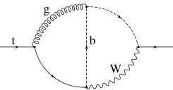
(a)	(b)
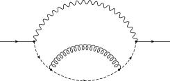
(c)	(d)

Figure 1: Diagrams whose imaginary parts determine the top width: Born level (a), and ${\cal O}(\alpha_{s})$ corrections (b,c,d).

To order $\alpha_{s}$ the width of the top quark is given by the diagrams in Fig. 1. The limit of a very heavy top is taken by neglecting $b$ mass and replacing the $W$ propagator by

$$i{p^{\mu}p^{\nu}\over p^{2}}{1\over M_{W}^{2}}.$$ (8)

The tree level width (diagram 1(a)) is

$$\Gamma^{0}={G_{F}m^{3}\over 8\sqrt{2}\pi}\left[1+\epsilon(2-\ln m^{2})\right].$$ (9)

The calculation was performed in $D=4-2\epsilon$ dimensions and the ${\cal O}(\epsilon)$ term is needed for the renormalization of the ${\cal O}(\alpha_{s})$ correction as described below.

The one-loop QCD correction consists of the Born width multiplied by the wave function renormalization constant $Z_{2}$ plus contributions of diagrams (b,c,d). For $Z_{2}$ we find ($C_{F}=4/3$):

$$Z_{2} = C_{F}{g^{2}\over 16\pi^{2}}M^{-2\epsilon}\left[-{1\over\epsilon}+1+\left(1+{3\over\delta^{2}}+{8\over\delta^{3/2}}\right)\ln(1-\delta)+{3\over\delta}+{8\over\delta^{1/2}}\right]$$ (10)

$$= C_{F}{g^{2}\over 16\pi^{2}}M^{-2\epsilon}\left[-{1\over\epsilon}-{1\over 2}-\sum_{n=1}{\delta^{n}\over n}-3\sum_{n=1}{\delta^{n}\over n+2}+{8\over\sqrt{\delta}}\sum_{n=1}{\delta^{n}\over n+1}\right]$$

If we pull out a factor $m^{3}g_{s}^{2}e^{2}C_{F}/(256\pi^{3}s_{W}^{2}M_{W}^{2})$ the contributions of the diagrams (b,c,d) to the width are

$$\Gamma_{b} = {1\over 2\epsilon}-{1\over 2}\ln m^{2}-{1\over 2}\ln M^{2}+{3\over 4}-\sum_{n=2}\left({2(2n^{2}-1)\over(n^{2}-1)n^{2}}-{1\over n}\ln\delta\right)\delta^{n-3/2}$$

$$+3\sum_{n=2}{1\over(n+2)(n+1)n(n-1)}\delta^{n-1},$$

$$\Gamma_{c} = \sum_{n=1}\left({2n-1\over 2(n+1)(n+3)}-{2n\over(n+2)(n+3)}\sqrt{\delta}\right)\delta^{n},$$

$$\Gamma_{d} = -{1\over 4\epsilon}+{1\over 2}\ln m^{2}-{29\over 24}.$$ (11)

After adding all four contributions and taking $\delta=1$ we find

$$\Gamma^{(1)} = {C_{F}g_{s}^{2}e^{2}m^{3}\over s_{W}^{2}M_{W}^{2}}{1\over 2^{9}\pi^{3}}\left[-{13\over 6}+4\sum_{n=1}{n^{2}-n-1\over n(n+1)^{2}(n+2)}\right.$$ (12)

$$\left.-3\sum_{n=2}{2n^{2}-3\over(n^{2}-1)n(n+2)}\right]={G_{F}m^{3}\over\sqrt{2}}{C_{F}\alpha_{s}\over 16\pi^{2}}\left({5\over 2}-{2\pi^{2}\over 3}\right).$$

The two sums in the above formula correspond to terms odd and even in $\sqrt{\delta}$, respectively. In obtaining them one has to shift the summation index so that equal powers of $\delta$ are added together. We see that we have correctly reproduced the result for the one-loop correction to $t\to bW$. [24]

5 Summary

We have reviewed our recent calculations of the second order corrections to processes involving heavy quarks. The techniques we have developed can be applied in many situations where the radiating particles can be considered non-relativistic. We have also demonstrated that some relativistic calculations can also be performed if sufficiently many expansion terms are available. Finally, we have discussed some recent results on semileptonic decays of the heavy quark into a massless quark in the final state.

References

References

- [1] I. Bigi, M. Shifman, and N. Uraltsev, Ann. Rev. Nucl. Part. Sci. 47, 591 (1997).
-
[2]
F. V. Tkachev, Sov. J. Part. Nucl. 25, 649 (1994)
[hep-ph/9701272].
V. A. Smirnov, Mod. Phys. Lett. A 10, 1485 (1995) [hep-th/9412063]. - [3] K. G. Chetyrkin and F.V. Tkachov, Nucl. Phys. B 192, 159 (1981).
- [4] D. J. Broadhurst, Z. Phys. C 54, 599 (1992).
-
[5]
V. A. Smirnov, Phys. Lett. B 394, 205 (1997).
A. Czarnecki and V. A. Smirnov, Phys. Lett. B 394, 211 (1997). - [6] A. Czarnecki and K. Melnikov, Phys. Rev. D 56, 7216 (1997).
- [7] A. Czarnecki and K. Melnikov, Phys. Rev. Lett. 78, 3630 (1997).
- [8] A. Czarnecki and K. Melnikov, hep-ph/9804215.
- [9] A. Czarnecki Phys. Rev. Lett. 76, 4124 (1996); A. Czarnecki and K. Melnikov, Nucl. Phys. B 505, 65 (1997).
- [10] S. J. Brodsky, G. P. Lepage, and P. B. Mackenzie, Phys. Rev. D 28, 228 (1983).
- [11] M. Neubert, Phys. Lett. B 341, 367 (1995).
- [12] M. Luke, M. J. Savage, and M. B. Wise, Phys. Lett. B 345, 301 (1995).
- [13] P. Ball and M. Beneke and V. M. Braun, Phys. Rev. D 52, 3929 (1995).
- [14] P. Ball and M. Beneke, private communication.
- [15] N. G. Uraltsev, Int. J. Mod. Phys. A 11, 515 (1996).
- [16] M. Beneke and V. M. Braun, Phys. Lett. B 348, 513 (1995).
- [17] A. Czarnecki, K. Melnikov and N. Uraltsev, Phys. Rev. Lett. 80, 3189 (1998).
- [18] N. G. Uraltsev, lectures given at Intl. School of Physics “Enrico Fermi,” Varenna, Italy, 1997; hep-ph/9804275.
- [19] A. Czarnecki, K. Melnikov and N. Uraltsev, Phys. Rev. D 57, 1769 (1998).
- [20] I. Bigi, M. Shifman, N. Uraltsev and A. Vainshtein, Phys. Rev. D 56, 4017 (1997).
- [21] A. Czarnecki and K. Melnikov, hep-ph/9806244.
- [22] A. Czarnecki and J. H. Kühn, Phys. Rev. Lett. 77, 3955 (1996).
- [23] A. Czarnecki and K. Melnikov, Phys. Rev. D 56, 1638 (1997).
- [24] M. Jeżabek and J. H. Kühn, Nucl. Phys. B 314, 1 (1989).