FZJ–IKP(TH)–1998–12

Strange magnetism in the nucleon

Thomas R. Hemmert,^‡ Ulf-G. Meißner,^‡ Sven Steininger^†,‡

^‡Forschungszentrum Jülich, IKP (Theorie), D–52425 Jülich, Germany

^†Department of Physics, Harvard University, Cambridge MA02138, USA

ABSTRACT

Using heavy baryon chiral perturbation theory to one loop, we derive an analytic and parameter–free expression for the momentum dependence of the strange magnetic form factor of the nucleon $G_{M}^{(s)}(Q^{2})$ and its corresponding radius. This should be considered as a lower bound. We also derive a model–independent relation between the isoscalar magnetic and the strange magnetic form factors of the nucleon based on chiral symmetry and SU(3) only. This gives an upper bound on the strange magnetic form factor. We use these limites to derive bounds on the strange magnetic moment of the proton from the recent measurement of $G_{M}^{(s)}(Q^{2}=0.1\,{\rm GeV}^{2})$ by the SAMPLE collaboration. We stress the relevance of this result for the on–going and future experimental programs at various electron machines.

PACS numbers: 13.40.Cs, 12.39.Fe, 14.20.Dh

1. There has been considerable experimental and theoretical interest concerning the question: How strange is the nucleon? Despite tremendous efforts, we have not yet achieved a detailled understanding about the strength of the various strange operators in the proton. These are $\bar{s}s$, as extracted from the analysis of the pion–nucleon $\Sigma$–term, $\bar{s}\gamma_{\mu}\gamma_{5}s$ as measured e.g. in deep–inelastic lepton scattering off protons and the vector current $\bar{s}\gamma_{\mu}s$, which is accesible e.g. in parity–violating electron–nucleon scattering. A dedicated program at Jefferson Laboratory preceded by experiments at BATES (MIT) and MAMI (Mainz) is aimed at measuring the form factors related to the strange vector current. In fact, the SAMPLE collaboration has recently reported the first measurement of the strange magnetic moment of the proton [1]. To be precise, they give the strange magnetic form factor at a small momentum transfer, $G_{M}^{(s)}(q^{2}=-0.1~{}{\rm GeV}^{2})=+0.23\pm 0.37\pm 0.15\pm 0.19\,$nuclear magnetons (n.m.). The rather sizeable error bars document the difficulty of such type of experiment. On the theoretical side, there is as much or even more uncertainty. To document this, let us pick one particular approach. Jaffe [2] deduced rather sizeable strange vector current matrix elements from the dispersion–theoretical analysis of the nucleon electromagnetic form factors, assuming that the isoscalar spectral functions are dominated at low momentum transfer by the $\omega$ and $\phi$ mesons. This analysis was updated in [3] with similar results. However, if one improves the isoscalar spectral function by considering also the correlated $\pi\rho$–exchange [4] or kaon loops [5], the corresponding strange matrix elements can change dramatically. Also, the spread of the theoretical predictions for the strange magnetic moment, $-0.8\leq\mu_{p}^{(s)}\leq 0.5$ n.m. underlines clearly the abovemade statement (for a review, see ref.[6]). As we will demonstrate in the following, there is, however, one quantity of reference, namely we can make a parameter–free prediction for the momentum dependence of the nucleons’ strange magnetic (Sachs) form factor based on the chiral symmetry of QCD solely. In addition, we derive a leading order model–independent relation between the strange and the isoscalar magnetic form factors, which allows to give an upper bound on the momentum dependence of $G_{M}^{(s)}(Q^{2})$. These two different results can then be combined to extract a range for the strange magnetic moment of the proton from the SAMPLE measurement of the form factor at low momentum transfer.

2. The strangeness vector current of the nucleon is defined as

$$\langle N|\;\bar{s}\;\gamma_{\mu}\;s\;|N\rangle=\langle N|\;\bar{q}\;\gamma_{\mu}\;(\lambda^{0}/3-\lambda^{8}/\sqrt{3})\;q\;|N\rangle=(1/3)J_{\mu}^{0}-(1/\sqrt{3})J_{\mu}^{8}\;,$$ (1)

with $q=(u,d,s)$ denoting the triplet of the light quark fields and $\lambda^{0}=I\;(\lambda^{a})$ the unit (the $a=8$ Gell–Mann) SU(3) matrix. Assuming conservation of all vector currents, the corresponding singlet and octet vector current for a spin–1/2 baryon can then be written as (from here on, we mostly consider the nucleon)

$$J_{\mu}^{0,8}=\bar{u}_{N}(p^{\prime})\left[F_{1}^{(0,8)}(q^{2})\gamma_{\mu}+F_{2}^{(0,8)}(q^{2})\frac{i\sigma_{\mu\nu}q^{\nu}}{2m_{N}}\right]u_{N}(p)\;.$$ (2)

Here, $q_{\mu}=p^{\prime}_{\mu}-p_{\mu}$ corresponds to the four–momentum transfer to the nucleon by the external singlet ($v_{\mu}^{(0)}=v_{\mu}\lambda^{0}$) and the octect ($v_{\mu}^{(8)}=v_{\mu}\lambda^{8}$) vector source $v_{\mu}$, respectively. The strangeness Dirac and Pauli form factors are defined via:

$$F_{1,2}^{(s)}(q^{2})=\frac{1}{3}F_{1,2}^{(0)}(q^{2})-\frac{1}{\sqrt{3}}F_{1,2}^{(8)}(q^{2})\;,$$ (3)

subject to the normalization $F_{1}^{(s)}(0)=S_{B}$, with $S_{B}$ the strangeness quantum number of the baryon ($S_{N}=0$) and $F_{2}^{(s)}(0)=\kappa_{B}^{(s)}$, with $\kappa_{B}^{(s)}$ the (anomalous) strangeness moment. In the following we concentrate our analysis on the “magnetic” strangeness form factor $G_{M}^{(s)}(q^{2})$, which in analogy to the (electro)magnetic Sachs form factor is defined as

$$G_{M}^{(s)}(q^{2})=F_{1}^{(s)}(q^{2})+F_{2}^{(s)}(q^{2})~{}.$$ (4)

It is this “strangeness” form factor for which chiral perturbation theory (CHPT) gives the most interesting predictions. Furthermore, $G_{M}^{(s)}(q^{2})$ is also the strangeness form factor that figures prominently in the recent Bates measurement [1].

3. Heavy baryon chiral perturbation theory (HBCHPT) is a precise tool to investigate the low–energy properties of the nucleon. It has, however, been argued that due to the appearance of higher order local contact terms with undetermined coefficents, CHPT can not be used to make any prediction for the strange magnetic moment or the strange electric radius without additional, model–dependent assumptions [7]. However, the analysis of the nucleons electromagnetic form factors in CHPT shows that to one loop the slope of the isovector Pauli form factor can be predicted in a parameter–free manner, see refs.[8, 9, 10, 12]. Since to the same order the corresponding isoscalar piece is a constant, one therefore has a parameter–free prediction for the radius of the Pauli form factor. It is thus natural to extend this calculation to the three flavor case with the appropriate singlet and octet currents as defined in Eq.(2).

We give here the relevant HBCHPT Lagrangians needed for the calculation. The baryon octet is parametrized in the matrix $B$, which has the usual transformation properties of any matter field under chiral transformation. We utilize the chiral covariant derivative $D_{\mu}$,

$$D_{\mu}B = \left(\partial_{\mu}+\Gamma_{\mu}-iv_{\mu}^{(0)}\right)B$$ (5)

$$\Gamma_{\mu} = \frac{1}{2}\left[u^{\dagger},\partial_{\mu}u\right]-\frac{i}{2}u^{\dagger}\left(v_{\mu}^{(i)}+a_{\mu}^{(i)}\right)u-\frac{i}{2}u\left(v_{\mu}^{(i)}-a_{\mu}^{(i)}\right)u^{\dagger}\;,\quad(i=3,8)$$ (6)

the chiral vielbein $u_{\mu}$,

$$u_{\mu} = i\;u^{\dagger}\nabla_{\mu}U\;u^{\dagger}$$ (7)

$$\nabla_{\mu}U = \partial_{\mu}U-i\left(v_{\mu}^{(i)}+a_{\mu}^{(i)}\right)U+iU\left(v_{\mu}^{(i)}-a_{\mu}^{(i)}\right),\quad(i=3,8)$$ (8)

where the quantities $v_{\mu}^{(x)}(a_{\mu}^{(x)})\;,x=0,3,8$ correspond to external vector (axial-vector) sources and $U(x)=u^{2}(x)$ parametrizes the octet of Goldstone bosons. The three flavor HBCHPT Lagrangian then reads (we only give the terms relevant to the calculations presented here)

$${\cal L}_{\rm MB}^{(1)} = \langle\bar{B}\;iv^{\mu}D_{\mu}\;B\rangle+D\;\langle\bar{B}\;S^{\mu}\{u_{\mu},B\}_{+}\rangle+F\;\langle\bar{B}\;S^{\mu}[u_{\mu},B]_{-}\rangle$$ (9)

$${\cal L}_{\rm MB}^{(2)} = -\frac{ib_{6a}^{F}}{4m_{N}}\;\langle\bar{B}\left[S^{\mu},S^{\nu}\right][f_{+\mu\nu}^{(3)},B]\rangle-\frac{ib_{6a}^{D}}{4m_{N}}\;\langle\bar{B}\left[S^{\mu},S^{\nu}\right]\{f_{+\mu\nu}^{(3)},B\}\rangle$$ (10)

$$-\frac{ib_{6b}^{F}}{4m_{N}}\;\langle\bar{B}\left[S^{\mu},S^{\nu}\right][f_{\+\mu\nu}^{(8)},B]\rangle-\frac{ib_{6b}^{F}}{4m_{N}}\;\langle\bar{B}\left[S^{\mu},S^{\nu}\right]\{f_{+\mu\nu}^{(8)},B\}\rangle$$

$$-\frac{2ib_{6c}}{4m_{N}}\;\langle\bar{B}\left[S^{\mu},S^{\nu}\right]v_{\mu\nu}^{(0)}\;B\rangle+\ldots$$

with

$$f_{+\mu\nu}^{(i)} = u^{\dagger}F_{\mu\nu}^{R\;(i)}u+uF_{\mu\nu}^{L\;(i)}u^{\dagger}$$ (11)

$$F_{\mu\nu}^{L,R\;(i)} = \partial_{\mu}F_{\nu}^{L,R\;(i)}-\partial_{\nu}F_{\mu}^{L,R\;(i)}-i\left[F_{\mu}^{L,R\;(i)},F_{\nu}^{L,R\;(i)}\right]$$ (12)

$$F_{\mu}^{R\;(i)} = v_{\mu}^{(i)}+a_{\mu}^{(i)}\quad\quad F_{\mu}^{L\;(i)}\;=\;v_{\mu}^{(i)}-a_{\mu}^{(i)}$$ (13)

$$v_{\mu\nu}^{(0)} = \partial_{\mu}v_{\nu}^{(0)}-\partial_{\nu}v_{\mu}^{(0)}~{},$$ (14)

where $\langle\ldots\rangle$ denotes the trace in flavor space and $m_{N}$ the nucleon mass. Furthermore, $F\simeq 1/2$ and $D\simeq 3/4$ are the conventional SU(3) axial coupling constants (in the chiral limit, to be precise). The dimension two terms are accompanied by finite low–energy constants (LECs), called $b_{6a}^{D,F},b_{6b}^{D,F},b_{6c}$. Their precise meaning will be discussed later.

4. To be specifc, we now consider the strange magnetic form factor to one loop order in CHPT. The strange magnetic moment of the nucleon gets renormalized by the kaon cloud, completely analogous to the renormalization of the nucleon isovector magnetic moment $\mu_{N}$ by the pion cloud [13, 10, 12, 14, 15]. It can be written as

$$\mu_{N}^{(s)}=\mu_{p}^{(s)}=\mu_{n}^{(s)}=\frac{1}{3}G_{M}^{(0)}(0)+\frac{1}{3}b_{6b}^{D}-b_{6b}^{F}+\frac{m_{N}M_{K}}{24\pi F_{\pi}^{2}}\left(5D^{2}-6DF+9F^{2}\right)~{},$$ (15)

with $M_{K}$ the kaon mass and $F_{\pi}\equiv(F_{\pi}+F_{K})/2\simeq 102\,$MeV the average pseudoscalar decay constant. We use this value because the difference between the pion and the kaon decay constants only shows up at higher order. One finds that to ${\cal O}(p^{3})$ in the chiral calculation the strange magnetic moments of the proton and the neutron are predicted to be equal and consist of three distinct contributions. First, the singlet magnetic moment $G_{M}^{(0)}(0)$ is parametrized in terms of the unknown singlet coupling $b_{6c}$. It cannot be predicted without additional experimental input as has already been noted in [7]. The counterterms $b_{6b}^{D,F}$, however, can be extracted from the anomalous magnetic moments $\kappa_{p},\kappa_{n}$ of the proton and the neutron. Third, there is a strong renormalization of $\mu_{N}$ due to the kaon cloud. To ${\cal O}(p^{3})$ we find $\mu_{N}^{(s)\;{\rm K-loops}}=2.0$, which is large and positive. This result is in agreement with the calculation of ref.[7]. It is well–known that such large leading order kaon loop effects generally are diminished by higher order corrections (unitarization), see e.g. [4]. We also note that in some models the strange magnetic moment is assumed to be generated exclusively by the kaon contributions [16], which is already ruled out to leading order chiral analysis of Eq.(15).

To obtain the complete strange magnetic form factors one only has to consider the diagrams shown in Fig.1. For the loop graph 1a, in case of an incoming nucleon, the only allowed intermediate states are $K\Lambda$ and $K\Sigma$, i.e. the pion and the $\eta$ cloud do not contribute to this order.

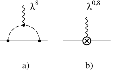
Figure 1: Coupling of the singlet ($\sim\lambda^{0}$) and octet ($\sim\lambda^{8}$) vector currents (wiggly line) to the nucleon (solid line). a) is a one kaon (dashed line) loop graph and b) a dimension two contact term. The latter only contributes to the strange magnetic moment.

For the proton ($p$) and the neutron ($n$) one finds

$$G_{M}^{(s)}(Q^{2}) = G_{M}^{(s)\;p}(Q^{2})\;=\;G_{M}^{(s)\;n}(Q^{2})$$ (16)

$$= \mu_{N}^{(s)}+\frac{\pi m_{N}M_{K}}{(4\pi F_{\pi})^{2}}\;\frac{2}{3}\left(5D^{2}-6DF+9F^{2}\right)\,f(Q^{2})~{},$$

with $Q^{2}=-q^{2}$. The momentum dependence is given entirely in terms of

$$f(Q^{2})=-\frac{1}{2}+\frac{4+Q^{2}/M_{K}^{2}}{4\sqrt{Q^{2}/M_{K}^{2}}}\arctan\biggl{(}\frac{\sqrt{Q^{2}}}{2M_{K}}\biggr{)}~{}.$$ (17)

The function $f(Q^{2})$ is shown in Fig.2. For small and moderate $Q^{2}$, it rises almost linearly with increasing $Q^{2}$.

Figure 2: The function $f(Q^{2})$ for small and moderate momentum transfer squared.

We note from Eq.(16) that the slope of $G_{M}^{(s)}(Q^{2})$ is uniquley fixed in terms of well–known low energy parameters,

$$\left(\rho_{M}\right)^{2}=\frac{d\;G_{M}^{(s)}(q^{2})}{dq^{2}}\biggl{|}_{q^{2}=0}=-\frac{\pi m_{N}}{(4\pi F_{\pi})^{2}M_{K}}\;\frac{1}{18}\left(5D^{2}-6DF+9F^{2}\right)=-0.027\,\mbox{fm}^{2}~{}.$$ (18)

The slope is identical for a proton or a neutron target, it is negative and to this order independent of the the strange magnetic moment $\mu_{N}^{(s)}$. The radius has the very reasonable behavior that in the limit of very heavy kaons, $M_{K}\rightarrow\infty$, it goes to zero, whereas it explodes in the chiral limit $M_{K}\rightarrow 0$. This quantity allows one to obtain the strange magnetic moment measured at a small value of $Q^{2}$ by linear extrapolation to $Q^{2}=0$. Note, however, that the value given should be considered as a lower limit. From an analysis of the electromagnetic form factors of the nucleon we know that at low momentum transfer the leading CHPT predictions are already quite satisfactory. However, in the SU(2) “small scale expansion framework” [11] it was found [12] that the radius of the isovector magnetic Sachs form factor $G_{M}^{I=1}(q^{2})$ is increased by 15-20% due to intermediate $\Delta\pi$ cloud effects. As similar analysis in the SU(3) “small scale expansion” framework is in preparation to see whether there are similarly sizeable corrections for the magnetic strangeness form factor due to intermediate decuplet-octet states. In addition, there are other mechanisms (like e.g. contributions from vector mesons) not covered at this order.

5. We can also give an upper limit for the strange magnetic form factor as the following arguments shows. For that, we consider the electromagnetic current

$$J_{\mu}^{\rm EM} = \langle N|\frac{2}{3}\bar{{\it u}}\gamma_{\mu}{\it u}-\frac{1}{3}\bar{{\it d}}\gamma_{\mu}{\it d}-\frac{1}{3}\bar{{\it s}}\gamma_{\mu}{\it s}|N\rangle$$ (19)

$$= \frac{1}{2\sqrt{3}}\langle N|\bar{q}\gamma_{\mu}\lambda_{8}q|N\rangle+\frac{1}{2}\langle N|\bar{q}\gamma_{\mu}\lambda_{3}q|N\rangle$$

$$= \frac{1}{2\sqrt{3}}J_{\mu}^{8}+\frac{1}{2}J_{\mu}^{3}\;,$$

where $J_{\mu}^{8}$ corresponds to the octet current of Eq.(1). The (conserved) triplet current $J_{\mu}^{3}$ parameterizes the response of a nucleon coupled to an external triplet vector source $v_{\mu}^{(3)}=v_{\mu}\lambda^{3}$. The calculation proceeds as before. We find that while in an SU(3) calculation the magnetic form factors of the proton and the neutron both have a pion and a kaon cloud contribution, the pion cloud terms drop out to leading order for the isoscalar magnetic form factor of the nucleon. Also, in contrast to the SU(2) calculations [10, 12], the leading one loop SU(3) contribution to $G_{M}^{I=0}(Q^{2})$ picks up a momentum dependence given again entirely in terms of the function $f(Q^{2})$, see Eq.(17),

$$G_{M}^{I=0}(Q^{2})^{SU(3)} = G_{M}^{p}(Q^{2})+G_{M}^{n}(Q^{2})$$ (20)

$$= \mu_{s}-\frac{M_{K}m_{N}\pi}{(4\pi F_{\pi})^{2}}\;\frac{2}{3}\left(5\;D^{2}-6\;D\;F+9\;F^{2}\right)\,f(Q^{2})~{},$$

with $\mu_{s}=0.88\,$n.m. the isoscalar nucleon magnetic moment. We note that to this order in the chiral expansion the prediction is again free of counterterms for the momentum dependence. Interestingly, this means that to ${\cal O}(p^{3})$ the isoscalar magnetic form factor of the nucleon is completely dominated by the kaon cloud, as all virtual pion contributions cancel exactly to this order. The result is of course consistent with the SU(2) analyses of [10, 12] as one can check that $G_{M}^{I=0}(Q^{2})\rightarrow\mu_{s}$ in the limit $M_{K}\rightarrow\infty$, i.e. the kaon cloud contribution shows up via higher order counterterms in the SU(2) calculation. For the leading chiral contribution to the isoscalar magnetic radius one finds

$$\left(r_{M}^{I=0}\right)^{2}=\frac{6}{\mu_{s}}\;\frac{d\;G_{M}^{I=0}(q^{2})}{dq^{2}}\biggl{|}_{q^{2}=0}=\frac{\left(5D^{2}-6DF+9F^{2}\right)m_{N}}{48F_{\pi}^{2}\mu_{s}\pi M_{K}}=0.18\,\mbox{fm}^{2}~{},$$ (21)

which is about 27% of the radius derived from the empirical dipole parametrization (notice that for the accuracy discussed here, we do not need to employ more sophisticated parametrizations as e.g. given in ref.[17]). It should now be clear that the isoscalar magnetic form factor and the strangeness magnetic form factor of the nucleon are closely related. In CHPT one can establish this connection on a firm ground. Based on the results obtained so far, we can derive in addition to the counterterm–free prediction of the low $Q^{2}$-dependence of $G_{M}^{(s)}$ in Eq.(16) another model-independent relation between the isoscalar magnetic form factor $G_{M}^{I=0}(q^{2})$ of the nucleon and the strange magnetic form factor:

$$G_{M}^{(s)}(Q^{2})=\mu_{N}^{(s)}+\mu_{s}-G_{M}^{I=0}(Q^{2})+{\cal O}(p^{4})$$ (22)

This relation is exact to ${\cal O}(p^{3})$ in SU(3) heavy baryon CHPT. Possible corrections in higher orders can be calculated systematically. This relation does not constrain $G_{M}^{(s)}(0)=\mu_{N}^{(s)}$, but makes new predictions on its $Q^{2}$-dependence. Utilizing the dipole parameterization for $G_{M}^{I=0}(Q^{2})$ one finds

$$\left(\rho_{M}^{(s),\;{\rm dip}}\right)^{2}=-\frac{d\;G_{M}^{I=0,\;{\rm dip}}(q^{2})}{dq^{2}}\biggr{|}_{q^{2}=0}=-0.10\,\mbox{fm}^{2}~{}.$$ (23)

This number is roughly three times larger than the leading chiral estimate of Eq.(18). Given that there are also non–strange contributions in the isoscalar magnetic form factor, which will start to manifest at order $q^{4}$, we consider Eq.(23) as an upper bound on the strange magnetic radius. The corresponding strange magnetic form factor is shown in Fig.3 for a vanishing strange magnetic moment and using the dipole parametrization for the isoscalar magnetic form factor. Any finite value for $\mu_{N}^{(s)}$ can be accomodated by simply shifting the curve up or down the abzissa. Note that a similar dipole–like behaviour with a much smaller slope (corresponding to the lower bound discussed before) was found in the vector meson dominance type analysis supplemented by regulated kaon loops presented in ref.[18]. It is also important to note that chiral physics dominates the strange magnetic form factor at low momentum transfer. However, the steady increase in $G_{M}^{(s)}(Q^{2})$ will eventually be taken over by pole contributions as e.g. exploited in refs.[2, 3] leading to a fall–off at large $Q^{2}$. At which momentum transfer that will happen depends on the detailed dynamics and can only be worked out in specific models, see e.g. [18]. Note that the G0 collaboration will probe this particular range of momentum transfer [19].

Figure 3: The strange magnetic form factor derived from the isoscalar magnetic one with $\mu_{N}^{(s)}=0$.

One can now utilize the $Q^{2}$–dependence from the two bounds, Eqs.(16,23), to extract the strange magnetic moment from the SAMPLE result for the strange magnetic form factor. For $Q^{2}=0.1\,$GeV², the correction is -0.06 (using $F_{\pi}=102\,$MeV) and -0.20, respectively, i.e. for the mean value of ref.[1] we get

$$\mu_{p}^{(s)}=0.03\ldots 0.18\,{\rm n.m.}~{},$$ (24)

which even for the upper value is a sizeable correction. It is amusing to note that the small value for $\mu_{p}^{(s)}$ is in agreement with the analysis presented in ref.[4]. Clearly, these numbers should only be considered indicative since (a) the experimental errors are bigger than the correction and (b) higher order corrections to the relations derived here should be worked out.

6. In summary, we have derived two novel relations which constrain the momentum dependence of the strange magnetic form factor in the low energy region. The first one is based on the observation that to one loop oder in three flavor chiral perturbation theory, the strange form factor picks up a momentum dependence which is free of unknown coupling constants, see Eq.(16). The second one rests upon the observation that the isoscalar magnetic form factor calculated in SU(3) also acquires a momentum dependence which can be related to the one of the strange magnetic form factor. This gives the model–independent relation shown in Eq.(23). These results, which should be considered as a lower and an upper bound, respectively, should help to sharpen the extraction of the strange magnetic moment from the measurement of the form factor at small and moderate momentum transfer. Clearly, the leading order results discussed here also need to be improved by a systematic calculation of the corresponding corrections. Such efforts are under way.

Acknowledgements

We would like to thank the participants of the N* workshop at Trento (ECT*) for helpful comments, especially Steve Pollock.

References

- [1] B. Mueller et al. (SAMPLE collaboration), Phys. Rev. Lett. 78, 3824 (1997).
- [2] R.L. Jaffe, Phys. Lett. B229, 275 (1989).
- [3] H.–W. Hammer, Ulf-G. Meißner and D. Drechsel, Phys. Lett. B367, 323 (1996).
- [4] Ulf-G. Meißner, V. Mull, J. Speth and J.W. Van Orden, Phys. Lett. B408, 381 (1997).
- [5] M.J. Ramsey–Musolf and H.-W. Hammer, Phys. Rev. Lett. 80, 2539 (1998); H.-W. Hammer and M.J. Ramsey–Musolf, Phys. Lett. B416, 5 (1998).
- [6] M.J. Musolf et al., Phys. Rep. 239, 1 (1994).
- [7] M.J. Ramsey-Musolf and H. Ito, Phys. Rev. C55, 3066 (1997).
- [8] M.A.B. Bég and A. Zepeda, Phys. Rev. D6, 2912 (1972).
- [9] J. Gasser, M.E. Sainio, and A. Svarc, Nucl. Phys. B307, 779 (1988).
- [10] V. Bernard, J. Kambor, N. Kaiser and Ulf-G. Meißner, Nucl. Phys. B388, 315 (1992).
- [11] T.R. Hemmert, B.R. Holstein and J. Kambor, Phys. Lett. B395, 89 (1997); [hep-ph/9712496].
- [12] V. Bernard, H.W. Fearing, T.R. Hemmert and Ulf-G. Meißner, Nucl. Phys. A635 (1998), in press.
- [13] D.G. Caldi and H. Pagels, Phys. Rev. D10, 3739 (1974).
- [14] E. Jenkins, M. Luke, A.V. Manohar and M. Savage, Phys. Lett. B302, 482 (1993); ibid B388, 866 (E) (1996).
- [15] Ulf-G. Meißner and S. Steininger, Nucl. Phys. B499, 349 (1997).
- [16] W. Koepf, E.M. Henley and S.J. Pollock, Phys. Lett. B288, 11 (1992); M.J. Musolf and M. Burkardt, Z. Phys. C61, 433 (1994).
- [17] P. Mergell, Ulf-G. Meißner and D. Drechsel, Nucl. Phys. A596, 367 (1996).
- [18] H. Forkel, M. Nielsen, X. Jin and T.D. Cohen, Phys. Rev. C50, 3108 (1994).
- [19] TJNAF experiment E91-017 (D. Beck, spokesperson).