QCD Anomalous Structure of Electron

Abstract

The parton content of the electron is analyzed within perturbative QCD. It is shown that electron acquires an anomalous component from QCD, analogously to photon. The evolution equations for the ‘exclusive’ and ‘inclusive’ electron structure function are constructed and solved numerically in the asymptotic $Q^{2}$ region.

TPJU-13/98

I Introduction

The photon structure function describes the distribution of QCD partons inside a photon. It is known for long [1] to have ‘anomalous’ component, which is calculable within perturbative QCD and dominates at asymptotically large momentum scales. This asymptotic solution, as opposed to those for hadrons, is independent of input data measured at lower momentum scales. At finite scales the photon structure gets modified by both perturbative and non-perturbative QCD contributions.

The QCD structure of the photon is revealed in interactions with a highly virtual ‘probe’. To fix attention let us think of a virtual gluon $G^{*}$ with momentum $q$, probing the photon which gets resolved into QCD partons. Their density $f^{\gamma}_{k}(x,Q^{2})$ ($k=q,\bar{q},G$), depends on fractional momentum $x$ of the parton with respect to photon and on the gluon virtuality $Q^{2}=|q^{2}|$, which must be large as compared to the QCD scale $\Lambda_{\rm QCD}^{2}$.

The photon structure is measured in experiments where the electron serves as a target. The process is depicted in Fig. 1a, where also the notation is given. The black blob denotes ‘resolved’ photon and sums up all collinear QCD contributions. The full cross-section gets also a contribution from the hard (“direct”) $G^{*}\gamma$ scattering (see e.g. [2]), but we will not discuss it in this paper. Actually the photons emitted by the electron are virtual and, from the point of view of a physical process, $G^{*}$ measures the structure (parton content) of the electron, as depicted in Fig. 1b.

         

FIG. 1.: Deep inelastic scattering on a photon (a) and electron (b) target

The aim of this paper is to study the QCD predictions for the electron structure function at large momentum scales. In particular we will discuss the dependence on the maximal virtuality of intermediate photons emitted by the electron, i.e. on the maximal momentum transfer between final and initial electron. In the next section we present the problem in general and discuss the relation to experimentally measured quantities. In Sec. 3 we derive the QCD solution to the non-singlet electron structure function in the moments space. A complete set of evolution equations is constructed and solved in Sec. 4. In Sec. 5 we present the summary and outlook.

II General Framework

The space-like virtuality of the photon exchanged in the diagram in Fig. 1a

$$(p-p^{\prime})^{2}\equiv-P_{\gamma}^{2}$$ (1)

can be fixed by measuring the momentum $p^{\prime}$ of the outgoing electron. Otherwise it lies within kinematic limits

$$P^{2}_{\rm min}(y)\equiv m_{e}^{2}{y^{2}\over 1-y}\leq P_{\gamma}^{2}\leq Q^{2}{z+y-zy\over z},$$ (2)

where $m_{e}$ is the electron mass, $y=qp_{\gamma}/qp$ and $z=Q^{2}/2pq$ (these are approximate expressions valid at $P_{\gamma}^{2}\ll Q^{2}$ — the exact formulae can be found in [6]). Usually the upper limit on $P_{\gamma}^{2}$ is set by experimental conditions (e.g. by anti-tagging)

$$P_{\gamma}^{2}\leq P^{2}.$$ (3)

The density of partons ($k=q,\bar{q},G$) with momentum $p_{k}=zp$ seen by our probe in the electron reads

$$f^{e}_{k}(z,Q^{2},P^{2}) = \int dx\,dy\,\delta(z-xy)\!\!\!\!\int\limits_{P^{2}_{\rm min}(y)}^{P^{2}}\!\!\!\!\!dP_{\gamma}^{2}\;f^{e}_{\gamma}(y,P_{\gamma}^{2})f^{\gamma}_{k}(x,Q^{2},P_{\gamma}^{2})$$ (5)

$$= \int\limits_{z}^{1}{dy\over y}\int\limits_{P^{2}_{\rm min}(y)}^{P^{2}}\!\!\!\!\!dP_{\gamma}^{2}f^{e}_{\gamma}(y,P_{\gamma}^{2})f^{\gamma}_{k}({z\over y},Q^{2},P_{\gamma}^{2}),$$ (6)

where

$$f^{e}_{\gamma}(y,P_{\gamma}^{2})={\alpha_{\rm em}\over 2\pi}{1\over P^{2}_{\gamma}}\left[{1+(1-y)^{2}\over y}-2y{m_{e}^{2}\over P_{\gamma}^{2}}\right]$$ (7)

and $f^{\gamma}_{k}(x,Q^{2},P_{\gamma}^{2})$ describes the $G^{*}\gamma$ interaction. In Eq.(7) only transverse photons are taken into account which is correct within the leading order of perturbative QCD. All QCD contributions are contained in $f^{\gamma}_{k}(x,Q^{2},P_{\gamma}^{2})$, which is discussed in the literature as the structure function of virtual photon [4, 2, 3]. In the following we will assume that $P^{2}\gg m_{e}^{2}$ which allows us to neglect the second term in the square brackets of Eq.(7).

For $Q^{2}\gg P^{2}$ $f^{\gamma}_{k}(x,Q^{2},P_{\gamma}^{2})$ can be approximated by the structure function of real photon ($P_{\gamma}^{2}=0$) and upon integration over $P_{\gamma}^{2}$ we arrive at the Weizsäcker-Williams [5] formula:

$$f^{e}_{k}(z,Q^{2},P^{2})\approx\int\limits_{z}^{1}{dy\over y}\hat{f}^{e}_{\gamma}(y)f^{\gamma}_{k}({z\over y},Q^{2},0)\;\log{P^{2}\over P^{2}_{\rm min}(z)},$$ (8)

where

$$\hat{f}^{e}_{\gamma}(y)={\alpha_{\rm em}\over 2\pi}\,{1+(1-y)^{2}\over y}.$$ (9)

Formula (8) has probabilistic interpretation in terms of the density of photons emitted by the electron and the density of QCD partons within the photon. As discussed in [6], this partonic picture breaks down at very high energies when $Z$ and $W$ bosons contribute.

In general, the experimentally measured electron structure function is always integrated over a range of photon virtualities and summed over the contributions from all weak intermediate bosons. This structure function describes the QCD content of a real (on-shell) electron and allows for probabilistic interpretation of the cross sections. Even when we neglect the contributions from $Z$ and $W$ bosons the integration over $P_{\gamma}^{2}$ disables the partonic interpretation [7]. As compared to the standard QCD structure functions the electron one has extra dependence on maximal photon virtuality $P^{2}$, which means that we do not integrate over all final electron states. In this sense we say that this electron structure function is ‘exclusive’.

Eq.(8) is an approximation to the electron structure function for $Q^{2}\gg P^{2}$. The approach to this limit within QCD is discussed in the next section.

In the following we will assume that the $Z$ and $W$ bosons do not contribute but we will allow for arbitrary $P^{2}\leq Q^{2}$. For both $Q^{2}$ and $P^{2}$ much greater than $m_{e}^{2}$ we have (c.f. Eq.(3))

$$f^{e}_{k}(Q^{2},P^{2})=\int\limits_{P^{2}_{\rm min}}^{P^{2}}\!{dP_{\gamma}^{2}\over P_{\gamma}^{2}}\hat{f}^{e}_{\gamma}\otimes f^{\gamma}_{k}(Q^{2},P_{\gamma}^{2}),$$ (10)

with explicit $z$ dependence suppressed and $\otimes$ denoting convolution

$$(f\otimes g)(z)\equiv\int\limits_{0}^{1}dx\int\limits_{0}^{1}dy\,\delta(z-xy)\,f(x)g(y).$$ (11)

We know from experiment that a nearly real photon ($P^{2}_{\gamma}\ll\Lambda_{\rm QCD}^{2}$) has a hadronic component which is often described phenomenologically in terms of the Vector Meson Dominance model (VDM) (see e.g. [2, 3] and references therein). This non-perturbative hadronic component becomes less important at higher $Q^{2}$. As will be shown in the next section, any perturbative QCD predictions for $P_{\gamma}^{2}$ dependence require $P_{\gamma}^{2}>\Lambda_{\rm QCD}^{2}$ and this is the region we will consider in details. To this end we split the integral over $P_{\gamma}^{2}$ in Eq.(10) into $\int_{P_{\rm min}^{2}}^{P_{0}^{2}}+\int_{P_{0}^{2}}^{P^{2}}$ with some $P_{0}^{2}>\Lambda_{\rm QCD}^{2}$. In the first integral we use the VDM-like photon structure function, while the whole dependence on $P^{2}$ is contained in the second one:

$$f^{e}_{k}(Q^{2},P^{2}) = \hat{f}^{e}_{\gamma}\otimes\int\limits_{P_{\rm min}^{2}}^{P_{0}^{2}}\!{dP_{\gamma}^{2}\over P_{\gamma}^{2}}f^{\rm(V)}_{k}(Q^{2},P_{\gamma}^{2})$$ (13)

$$+\hat{f}^{e}_{\gamma}\otimes\int\limits_{P_{0}^{2}}^{P^{2}}\!{dP_{\gamma}^{2}\over P_{\gamma}^{2}}f^{\gamma}_{k}(Q^{2},P_{\gamma}^{2}).$$

III QCD calculation of electron structure function

From the theoretical point of view the QCD behavior of structure functions is most easily analyzed in terms of their moments, defined as

$$f(n)=\int\limits_{0}^{1}dx\,x^{n-1}f(x)$$ (14)

for any function $f$.

The electron structure function we are going to investigate has the form of the second term of Eq.(13) and its moments read

$$f^{e}_{k}(n,t,t_{1},t_{0})=\hat{f}^{e}_{\gamma}(n)\int\limits_{t_{0}}^{t_{1}}\!dt_{\gamma}f^{\gamma}_{k}(n,t,t_{\gamma}),$$ (15)

where

$$t=\log{Q^{2}\over\Lambda_{\rm QCD}^{2}}\;,\;\;t_{0}=\log{P_{0}^{2}\over\Lambda_{\rm QCD}^{2}}\;,\;\;t_{1}=\log{P^{2}\over\Lambda_{\rm QCD}^{2}}\;,\;\;t_{\gamma}=\log{P_{\gamma}^{2}\over\Lambda_{\rm QCD}^{2}}$$ (16)

and explicit $t_{0}$ argument of $f^{e}_{k}(n,t,t_{1},t_{0})$ is to remind on the dependence on ‘auxiliary’ scale $P_{0}^{2}$.

Our task will be to integrate $f^{\gamma}_{k}(n,t,t_{\gamma})$ over $t_{\gamma}$ and to construct master equations for the electron structure function. In order to introduce notation and get some understanding of the energy scales involved, let us first briefly remind the derivation of the virtual photon structure function.

The master (DGLAP) equations [8] read

$${df^{\gamma}_{q/\bar{q}}(n,t,t_{\gamma})\over dt} = {\alpha_{\rm em}\over 2\pi}e_{q}^{2}\hat{P}_{q\gamma}(n)$$ (18)

$$+ {\alpha\over 2\pi}P_{qq}(n)f^{\gamma}_{q/\bar{q}}(n,t,t_{\gamma})+{\alpha\over 2\pi}P_{qG}(n)f^{\gamma}_{G}(n,t,t_{\gamma}),$$ (19)

$${df^{\gamma}_{G}(n,t,t_{\gamma})\over dt} = {\alpha\over 2\pi}P_{Gq}(n)\sum_{q=1}^{n_{\rm f}}\left[f^{\gamma}_{q}(n,t,t_{\gamma})+f^{\gamma}_{\bar{q}}(n,t,t_{\gamma})\right]$$ (20)

$$+ {\alpha\over 2\pi}P_{GG}(n)f^{\gamma}_{G}(n,t,t_{\gamma}),$$ (21)

where

$$\hat{P}_{q\gamma}(x)=3[x^{2}+(1-x)^{2}]$$ (22)

is the photon-quark splitting function and $P_{ik}$ are the QCD (Altarelli–Parisi) splitting functions. In these equations the photon virtuality ($t_{\gamma}$) is fixed and can be thought of as an “external” parameter describing the state, QCD content of which depends on $t$ and $n$. The inhomogenous term in Eq.(18) makes the difference with QCD equations for hadrons.

The standard method of solving the evolution equations is to decompose first the structure functions into singlet and non-singlet components. To simplify the discussion we will present formulae for the non-singlet part only. Defining the non-singlet part of a structure function as

$$\bar{f}_{q/\bar{q}}=f_{q/\bar{q}}-{1\over 2n_{\rm f}}\sum_{q^{\prime}}^{n_{\rm f}}(f_{q}^{\prime}+f_{\bar{q}^{\prime}})$$ (23)

we obtain

$${d\bar{f}^{\gamma}_{q/\bar{q}}(n,t,t_{\gamma})\over dt}={\alpha_{\rm em}\over 2\pi}(e_{q}^{2}-\langle e_{q}^{2}\rangle)\hat{P}_{q\gamma}(n)+{\alpha\over 2\pi}P_{qq}(n)\bar{f}^{\gamma}_{q/\bar{q}}(n,t,t_{\gamma}),$$ (24)

where

$$\langle e_{q}^{2}\rangle={1\over 2n_{\rm f}}\sum_{q=1}^{n_{\rm f}}e_{q}^{2}$$ (25)

In the leading log order of QCD

$${\alpha(t)\over 2\pi}={2\over\beta_{0}t}$$ (26)

with $\beta_{0}=11-2n_{\rm f}/3$ for $n_{\rm f}$ flavors, and Eq.(24) becomes

$${d\bar{f}^{\gamma}_{q/\bar{q}}(n,t,t_{\gamma})\over dt}=\bar{d}_{q\gamma}(n)-{d_{qq}(n)\over t}\bar{f}^{\gamma}_{q/\bar{q}}(n,t,t_{\gamma}),$$ (27)

where

$$\bar{d}_{q\gamma}(n)={\alpha_{\rm em}\over 2\pi}(e_{q}^{2}-\langle e_{q}^{2}\rangle)\hat{P}_{q\gamma}(n)$$ (28)

and

$$d_{qq}(n)=-2{P_{qq}(n)\over\beta_{0}}\,.$$ (29)

The general solution to this differential equation reads

$$\bar{f}^{\gamma}_{q/\bar{q}}(n,t,t_{\gamma}) = {\bar{d}_{q\gamma}(n)\,t\over 1+d_{qq}(n)}\left[1-\left({t^{\prime}\over t}\right)^{1+d_{qq}(n)}\right]$$ (31)

$$+\bar{f}^{\gamma}_{q/\bar{q}}(n,t^{\prime},t_{\gamma})\,\left({t^{\prime}\over t}\right)^{d_{qq}(n)}$$

As shown for the first time by Witten [1], the first term is characteristic feature of the photon structure function and for large $t$ it dominates, resulting in linear growth with $t$. The second term in this solution depends on the ‘input’ measured at some $t^{\prime}$ and is analogous to the leading-log QCD evolution of hadronic structure functions. For low $t^{\prime}$ and $t_{\gamma}$ the measured structure function $\bar{f}^{\gamma}_{q/\bar{q}}(n,t^{\prime},t_{\gamma})$ can be identified with the VDM-like $\bar{f}^{\rm(V)}_{q/\bar{q}}(n,t^{\prime},t_{\gamma})$ discussed in the previous section.

Eq.(31) gives no explicit prediction on the $t_{\gamma}$ dependence of $\bar{f}^{\gamma}_{q/\bar{q}}(n,t,t_{\gamma})$ except for the fact that the asymptotic ($t\gg t^{\prime}$) solution is independent of $t_{\gamma}$

$$\bar{f}^{\gamma}_{q/\bar{q}}(n,t,t_{\gamma})\simeq{\bar{d}_{q\gamma}(n)\over 1+d_{qq}(n)}\,t.$$ (32)

Another method of calculating QCD structure functions is the ladder expansion. The corresponding diagram for the photon structure function is shown in Fig. 2a. Actual calculations should be performed in the axial gauge but here we will integrate only over the quark emitted by the photon, which is as simple as

$$\bar{f}^{\gamma}_{q/\bar{q}}(n,t,t_{\gamma})=\bar{d}_{q\gamma}(n)\int\limits_{P^{2}_{\gamma}}^{Q^{2}}{dk^{2}\over k^{2}}f_{qq}(n,Q^{2},k^{2}).$$ (33)

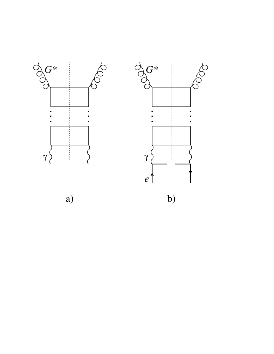
FIG. 2.: General ladder expansion for the photon (a) and the electron structure function (b)

The QCD ‘structure function of a point-like virtual quark’ $f_{qq}(n,Q^{2},k^{2})$ corresponds to the ladder diagram of Fig. 2a without the lowest quark rung. The latter is explicitly integrated in Eq.(33) with the electromagnetic $\gamma$-$q$ coupling contained in $\bar{d}_{q\gamma}(n)$ and $1/k^{2}$ coming from the quark propagator. The only difference with pure QCD is that here the coupling is electromagnetic and does not depend on $k^{2}$. Changing the integration variable to $\tau=\log(k^{2}/\Lambda_{\rm QCD}^{2})$ and using the QCD formula

$$f_{qq}(n,Q^{2},k^{2})=\left(\tau\over t\right)^{d_{qq}(n)}$$ (34)

we arrive at [4]

$$\bar{f}^{\gamma}_{q/\bar{q}}(n,t,t_{\gamma}) = \bar{d}_{q\gamma}(n)\int\limits_{t_{\gamma}}^{t}{d\tau}\left(\tau\over t\right)^{d_{qq}(n)}$$ (35)

$$= {\bar{d}_{q\gamma}(n)\,t\over 1+d_{qq}(n)}\left[1-\left({t_{\gamma}\over t}\right)^{1+d_{qq}(n)}\right].$$ (36)

Formally this result equals to the solution of master equations Eq.(31) with $t^{\prime}=t_{\gamma}$ and $\bar{f}^{\gamma}_{q/\bar{q}}(n,t_{\gamma},t_{\gamma})=0$.

Let us explain the implicit assumptions made in the derivation of Eq.(36). Thanks to the strong ordering of virtualities in the ladder expansion

$$P^{2}_{\gamma}<k^{2}<\dots<Q^{2}$$ (37)

we could integrate over the whole range of quark virtualities $k^{2}$. Within QCD, however, this can be done only if the photon virtuality $P^{2}_{\gamma}>\Lambda_{\rm QCD}^{2}$. Moreover we have used the fact that in perturbative calculation such photon has a point-like coupling to quarks. In other words the photon of virtuality $P^{2}_{\gamma}>\Lambda_{\rm QCD}^{2}$ has no QCD structure at the scale $Q^{2}=P^{2}_{\gamma}$. We see, thus, that Eq.(31) is valid for any $P^{2}_{\gamma}$ while Eq.(36) for $P^{2}_{\gamma}>\Lambda_{\rm QCD}^{2}$ only. This is exactly the reason for introducing the intermediate scale $P_{0}^{2}$ in Eq.(13).

In the following we will assume that $P^{2}_{\gamma}$ is large enough for Eq.(36) to hold. With this assumption the integration over $P^{2}_{\gamma}$, as in Eq.(15), is straightforward and results in the following expression for the electron structure function

$$\bar{f}^{e}_{q/\bar{q}}(n,t,t_{1},t_{0}) = \hat{f}^{e}_{\gamma}(n)\int\limits_{t_{0}}^{t_{1}}\!dt_{\gamma}\bar{f}^{\gamma}_{q/\bar{q}}(n,t,t_{\gamma})$$ (38)

$$= {\hat{f}^{e}_{\gamma}(n)\bar{d}_{q\gamma}(n)\,t\over 1+d_{qq}(n)}\Bigg{\{}t_{1}-t_{0}$$ (40)

$$-{t\over 2+d_{qq}(n)}\left[\left({t_{1}\over t}\right)^{2+d_{qq}(n)}-\left({t_{0}\over t}\right)^{2+d_{qq}(n)}\right]\Bigg{\}}.$$

This result corresponds to the diagram depicted in Fig. 2b, where the range of photon virtualities is controlled by imposing a limit on momentum transfer to the outgoing electron. Eq.(38) depends on three scales $t>t_{1}>t_{0}$ with $t_{0}$ kept fixed. In order to find formulae for large $t$ ($t\gg t_{0}$) we have to specify the relation between $t_{1}$ and $t$. Let us consider two extreme cases: $t_{1}\ll t$ and $t_{1}=t$.

• ‘Exclusive’ case: $t_{1}\ll t$

  $$\bar{f}^{e}_{q/\bar{q}}(n,t,t_{1},t_{0})\simeq{\hat{f}^{e}_{\gamma}(n)\bar{d}_{q\gamma}(n)\over 1+d_{qq}(n)}\,t(t_{1}-t_{0}).$$ (41)

• ‘Inclusive’ case: $t_{1}=t$

  $$\bar{f}^{e}_{q/\bar{q}}(n,t)\equiv\bar{f}^{e}_{q/\bar{q}}(n,t,t,t_{0})\simeq{\hat{f}^{e}_{\gamma}(n)\bar{d}_{q\gamma}(n)\over 2+d_{qq}(n)}\,t^{2},$$ (42)

  where we have dropped the last two arguments of the ‘inclusive’ structure function.

To obtain the full result for $\bar{f}^{e}_{q/\bar{q}}$ we still have to add the integral over the photon virtualities below $P_{0}^{2}$. To this end we use Eq.(31) with experimental input replaced by a VDM-like parametrization at $t^{\prime}=t_{0}$:

$$\bar{f}^{\gamma}_{q/\bar{q}}(n,t,t_{\gamma}) \approx {\bar{d}_{q\gamma}(n)\,t\over 1+d_{qq}(n)}\left[1-\left({t_{0}\over t}\right)^{1+d_{qq}(n)}\right]$$ (44)

$$+\bar{f}^{\rm(V)}_{q/\bar{q}}(n,t_{0},t_{\gamma})\,\left({t_{0}\over t}\right)^{d_{qq}(n)}.$$

As discussed earlier $\bar{f}^{\rm(V)}_{q/\bar{q}}(n,t_{0},t_{\gamma})$ should decrease with increasing $t_{\gamma}$ and vanish for $t_{\gamma}\geq t_{0}$ (see e.g. [3] for a phenomenological parametrization). Thus for $t\gg t_{0}$ we get the unique prediction independent of the ‘input’ at low $t_{0}$

$$\hat{f}^{e}_{\gamma}(n)\int\limits_{t_{\rm min}}^{t_{0}}\!dt_{\gamma}f^{\gamma}_{k}(n,t,t_{\gamma})\simeq{\hat{f}^{e}_{\gamma}(n)\bar{d}_{q\gamma}(n)\,t\over 1+d_{qq}(n)}(t_{0}-t_{\rm min}),$$ (45)

where $t_{\rm min}=\log(P_{\rm min}^{2}/\Lambda_{\rm QCD}^{2})$.

For large $t$ this low $P_{\gamma}^{2}$ contribution grows linearly with $t$ and can be neglected in the ‘inclusive’ case. Eq.(41) becomes now

$$\bar{f}^{e}_{q/\bar{q}}(n,t,t_{1})\simeq{\hat{f}^{e}_{\gamma}(n)\bar{d}_{q\gamma}(n)\over 1+d_{qq}(n)}\,t(t_{1}-t_{\rm min})\equiv{\hat{f}^{e}_{\gamma}(n)\bar{d}_{q\gamma}(n)\over 1+d_{qq}(n)}\,t\,\log{P^{2}\over P_{\rm min}^{2}}.$$ (46)

This is exactly the Weizsäcker-Williams formula Eq.(8) with asymptotic solution Eq.(32) used for the photon structure function.

Much more interesting is the ‘inclusive’ case Eq.(42). To understand this QCD prediction let us look first at the photon structure function. There the effect of QCD evolution can be seen by comparing the full result Eq.(36) with the Quark Parton Model (QPM) limit. We reach this limit by taking $\Lambda_{\rm QCD}^{2}\rightarrow 0$ ($\alpha(t)\rightarrow 0$) in Eq.(36), which results in

$$\bar{f}^{\gamma}_{q/\bar{q}}(n,t,t_{\gamma})|_{\rm QPM}=\bar{d}_{q\gamma}(n)\,(t-t_{\gamma})=\bar{d}_{q\gamma}(n)\,\log{Q^{2}\over P_{\gamma}^{2}}$$ (47)

Thus we see that for large $t$ the net effect of the QCD evolution on the photon structure function is to change $\bar{d}_{q\gamma}(n)$ into $\bar{d}_{q\gamma}(n)/(1+d_{qq}(n))$. The dependence on $t$ remains the same but the structure functions (transformed back to the $x$-space) have different dependence on $x$. As usually the QCD evolution ‘shifts’ the distribution towards lower $x$ values. Analogously, for the electron structure function the QPM limit of Eq.(38) reads

$$\bar{f}^{e}_{q/\bar{q}}(n,t,t_{1},t_{0})|_{\rm QPM} \simeq {\hat{f}^{e}_{\gamma}(n)\bar{d}_{q\gamma}(n)\over 2}(t_{1}-t_{0})(2t-t_{1}-t_{0})$$ (48)

$$= {\hat{f}^{e}_{\gamma}(n)\bar{d}_{q\gamma}(n)\over 2}\log{P^{2}\over P_{0}^{2}}\left(\log{Q^{2}\over P_{0}^{2}}+\log{Q^{2}\over P^{2}}\right)$$ (49)

The reader can easily check that this result corresponds to the integral $\int_{t_{0}}^{t_{1}}\!dt_{\gamma}$ of the QPM formula for the photon structure function, Eq.(47).

Comparing the QPM result with the QCD formulae Eq.(46) and Eq.(42) we see that the effect of QCD evolution is to multiply the moments of the electron structure function by $1/(1+d_{qq}(n))$ in the ‘exclusive’ case and by $2/(2+d_{qq}(n))$ in the ‘inclusive’ case. After transforming back to the $x$-space, this means that QPM, ‘exclusive’ and ‘inclusive’ electron structure functions all have different dependence on $x$. In particular the ‘inclusive’ solution $\bar{f}^{e}_{q/\bar{q}}(n,t)$, which corresponds to a standard structure function, gets modified analogously to the photon case but by another factor. In this sense the electron acquires an anomalous component from QCD.

So far we have discussed the non-singlet solution. The singlet case goes along the same lines but will not be presented here. Instead, we construct in the next section the evolution equations which can be solved in the $x$-space.

IV Evolution equations

Let us first show that Eq.(38) is the general solution to the following master equations

$${\partial\bar{f}^{e}_{q/\bar{q}}(n,t,t_{1},t_{0})\over\partial t} = d_{qe}(n)(t_{1}-t_{0})-{d_{qq}(n)\over t}\bar{f}^{e}_{q/\bar{q}}(n,t,t_{1},t_{0}),$$ (51)

$${\partial\bar{f}^{e}_{q/\bar{q}}(n,t,t_{1},t_{0})\over\partial t_{1}} = \hat{f}^{e}_{\gamma}(n)\bar{f}^{\gamma}_{q/\bar{q}}(n,t,t_{1})$$ (52)

$$= {d_{qe}(n)\,t\over 1+d_{qq}(n)}\left[1-\left({t_{1}\over t}\right)^{d_{qq}(n)+1}\right],$$ (53)

where $d_{qe}(n)\equiv\hat{f}^{e}_{\gamma}(n)\bar{d}_{q\gamma}(n)$. Note that the second equation is just the derivative of Eq.(13) with Eq.(36) inserted for the photon structure function. A general solution to Eq.(51) can be written as

$$\bar{f}^{e}_{q/\bar{q}}(n,t,t_{1},t_{0})=C(n,t_{1})\,t^{-d_{qq}(n)}+{d_{qe}(n)\over 1+d_{qq}(n)}\,(t_{1}-t_{0})t.$$ (54)

So far $C(n,t_{1})$ is an arbitrary function of $t_{1}$. Nb. if $t_{1}$ remains constant when $t\rightarrow\infty$ the second term of Eq.(54) gives the asymptotic solution for the ‘exclusive’ case.

From the second equation Eq.(52) we obtain

$$C(n,t_{1})=C^{(0)}(n)-{d_{qe}(n)\,t_{1}^{d_{qq}(n)+2}\over[1+d_{qq}(n)]\,[2+d_{qq}(n)]}$$ (55)

with arbitrary $C^{(0)}(n)$.

Now the general solution to Eq.(IV) reads

$$\bar{f}^{e}_{q/\bar{q}}(n,t,t_{1},t_{0}) = C^{(0)}(n)t^{-d_{qq}(n)}$$ (57)

$$+{d_{qe}(n)\over 1+d_{qq}(n)}\left[(t_{1}-t_{0})t-{t_{1}^{2+d_{qq}(n)}t^{-d_{qq}(n)}\over 2+d_{qq}(n)}\right].$$

Upon imposing the boundary condition $\bar{f}^{e}_{q/\bar{q}}(n,t,t_{0},t_{0})=0$ we recover the formula Eq.(38) derived in the previous section.

The complete set of master equations in the $x$-space analogous to Eq.(IV) can be obtained by changing the products of moments into convolutions and observing that there is no inhomogenous term for the gluonic component — c.f. Eq.(III). Suppressing explicit $t_{0}$ dependence in the function arguments we have

$${\partial f^{e}_{q/\bar{q}}(t,t_{1})\over\partial t} = {\alpha_{\rm em}\over 2\pi}\hat{P}_{qe}[t_{1}-t_{0}]$$ (60)

$$+{\alpha\over 2\pi}P_{qq}\otimes f^{e}_{q/\bar{q}}(t,t_{1})+{\alpha\over 2\pi}P_{qG}\otimes f^{e}_{G}(t,t_{1}),$$

$${\partial f^{e}_{q/\bar{q}}(t,t_{1})\over\partial t_{1}} = \hat{f}^{e}_{\gamma}\otimes f^{\gamma}_{q/\bar{q}}(t,t_{1}),$$ (61)

$${\partial f^{e}_{G}(t,t_{1})\over\partial t} = {\alpha\over 2\pi}P_{Gq}\otimes\sum_{q=1}^{n_{\rm f}}\left[f^{e}_{q}(t,t_{1})+f^{e}_{\bar{q}}(t,t_{1})\right]$$ (63)

$$+{\alpha\over 2\pi}P_{GG}\otimes f^{e}_{G}(t,t_{1}),$$

$${\partial f^{e}_{G}(t,t_{1})\over\partial t_{1}} = \hat{f}^{e}_{\gamma}\otimes f^{\gamma}_{G}(t,t_{1}),$$ (64)

where $\hat{P}_{qe}=\hat{P}_{q\gamma}\otimes\hat{f}^{e}_{\gamma}$.

These equations, as they stand, are not very useful because they contain both electron and photon structure functions. We will present now how a closed set of equations for the electron structure function is formed in the large $t$ region. As already discussed previously, the large $t$ limit depends on additional assumptions on $t_{1}$ vs. $t$ dependence. Quite generally one can take $t_{1}$ to be some function of $t$ defining a ‘path’ in the $t$-$t_{1}$ plane along which the large $t$ limit is approached. Denoting $t_{1}=g(t)$ we have

$${df^{e}_{k}(t,t_{1})\over dt} = {\partial f^{e}_{k}(t,t_{1})\over\partial t}+g^{\prime}(t){\partial f^{e}_{k}(t,t_{1})\over\partial t_{1}}$$ (65)

$$= {\partial f^{e}_{k}(t,t_{1})\over\partial t}+g^{\prime}(t)\hat{f}^{e}_{\gamma}\otimes f^{\gamma}_{k}(t,t_{1}).$$ (66)

A simple choice for $g(t)$ is

$$g(t)=(1-a)\hat{t}_{1}+at$$ (67)

where $\hat{t}_{1}$ is constant and $0\leq a\leq 1$. The two extreme cases considered in the previous section correspond to following choices for the parameter $a$

• ‘Exclusive’ case
  $a=0$, i.e. $g(t)=\hat{t}_{1}$. As $g^{\prime}(t)=0$ the second term in Eq.(66) vanishes. The solution grows linearly with $t$ (c.f. Eq.(3)). The resulting master equations have a constant ($t$-independent) inhomogenous term

  $${df^{e}_{q/\bar{q}}(t,\hat{t}_{1})\over dt} = {\alpha_{\rm em}\over 2\pi}\hat{P}_{qe}[\hat{t}_{1}-t_{0}]$$ (70)

  $$+{\alpha\over 2\pi}P_{qq}\otimes f^{e}_{q/\bar{q}}(t,\hat{t}_{1})+{\alpha\over 2\pi}P_{qG}\otimes f^{e}_{G}(t,\hat{t}_{1}),$$

  $${df^{e}_{G}(t,\hat{t}_{1})\over dt} = {\alpha\over 2\pi}P_{Gq}\otimes\sum_{q=1}^{n_{\rm f}}\left[f^{e}_{q}(t,\hat{t}_{1})+f^{e}_{\bar{q}}(t,\hat{t}_{1})\right]$$ (72)

  $$+{\alpha\over 2\pi}P_{GG}\otimes f^{e}_{G}(t,\hat{t}_{1})$$

• ‘Inclusive’ case.
  $a=1$, i.e. $g(t)=t$ and $g^{\prime}(t)=1$. Now the virtual photon structure function $f^{\gamma}_{k}(t,t)$ vanishes because both arguments are equal. We arrive at the equations which are formally the same as in the ‘exclusive’ case but with $\hat{t}_{1}$ set to $t$ and $t_{\rm min}$ neglected. The master equations have now the inhomogenous term proportional to $t$, which results in a different $x$-dependence of the solutions.

According to Eq.(41) and Eq.(42) the asymptotic solutions to these equations have the form

$$f^{e}_{k}(z,t)=\left({\alpha_{\rm em}\over 2\pi}\right)^{2}\tilde{f}^{e}_{k}(z)\,tt_{1}$$ (73)

with $t_{1}$ constant and $t_{1}=t$ for the ‘exclusive’ and ‘inclusive’ case, respectively. Here we have taken $t_{0}=0$ ($P_{0}^{2}=\Lambda_{\rm QCD}^{2}$). Substituting the leading-log formula Eq.(26) for $\alpha(t)$ we end up with $t$-independent integral equations

$$p\tilde{f}^{e}_{q/\bar{q}}(z) = \hat{P}_{qe}(z)+{2\over\beta_{0}}\int\limits_{z}^{1}\!{dx\over x}\left[P_{qq}(x)\tilde{f}^{e}_{q/\bar{q}}\!\left({z\over x}\right)+P_{qG}(x)\tilde{f}^{e}_{G}\!\left({z\over x}\right)\right]\!,$$ (75)

$$p\tilde{f}^{e}_{G}(z) = {2\over\beta_{0}}\int\limits_{z}^{1}\!{dx\over x}\sum_{k=q,\bar{q},G}P_{kq}(x)\tilde{f}^{e}_{k}\left({z\over x}\right),$$ (76)

where $p=1$ or $p=2$ for the ‘exclusive’ or ‘inclusive’ case, respectively.

FIG. 3.: Asymptotic $u$-quark ‘exclusive’ and ‘inclusive’ distributions $zf^{e}_{u}(z,Q^{2})/\alpha_{\rm em}^{2}$ for $Q^{2}=100{\rm GeV}^{2}$ and $P^{2}=1{\rm GeV}^{2}$ for ‘exclusive’ case. Calculations have been done for 5 flavors, $\Lambda_{\rm QCD}=0.2{\rm GeV}$ and $P_{0}^{2}=\Lambda_{\rm QCD}^{2}$.

We solve these equations numerically using the method described in [9]. In Fig. 3 we show the ‘exclusive’ and ‘inclusive’ solutions for the distribution of $u$ quarks in the electron at $Q^{2}=100{\rm GeV}^{2}$. There is still the contribution from the photons of low virtuality ($P_{\gamma}^{2}<\Lambda_{\rm QCD}^{2}$) which should be added, as it has been done in Eq.(46). At asymptotically large $t=\log(Q^{2}/\Lambda_{\rm QCD}^{2})$ it modifies the ‘exclusive’ solution only, by changing the $t_{1}=\log(P^{2}/\Lambda_{\rm QCD}^{2})$ factor in Eq.(73) into $\log(P^{2}/P_{\rm min}^{2})$. At finite $Q^{2}$, however, this contribution is non-negligible for ‘inclusive’ case and should also be added. As can be seen from Eq.(38) taking the intermediate scale $P_{0}^{2}=\Lambda_{\rm QCD}^{2}$ ($t_{0}=0$) sets the proper normalization for this correction at finite $t$. Thus the both curves in Fig. 3 get shifted by the same amount.

V Summary

In this paper we have analyzed the parton content of the electron within perturbative QCD. We have shown that electron acquires an anomalous component from QCD, analogously to photon. We have constructed the evolution equations for the ‘exclusive’ and ‘inclusive’ electron structure function. These two cases correspond to ‘anti-tagging’ and ‘no-tagging’ experimental conditions, respectively. The evolution equations can be solved numerically in the $x$-space in the asymptotic $Q^{2}$ region. As an example we have shown the $u$ quark distribution inside the electron.

The results presented here are leading-log QCD solutions valid at asymptotically large $Q^{2}$. At finite $Q^{2}$ the next-to-leading corrections, as well as non-perturbative contributions including hadronic component of the real photon will modify the results. Despite these inaccuracies it would be interesting to compare these predictions with experiment. On one hand, the data for the electron structure function should be much more precise than the ones used for the photon structure function. On the other hand, the improvements on the theoretical side can be done in a similar way as for the photon structure function — higher order perturbative QCD effects, as well as phenomenological parametrizations can be plugged into the evolution equations Eq.($\bullet$ ‣ IV).

The author would like to thank Jerzy Szwed for numerous discussions and for critical reading of the manuscript. The hospitality of DESY Theory group, where part of this work was done, is also acknowledged.

REFERENCES

• [1] E. Witten, Nucl. Phys. B120, 189 (1977); C.H. Llewellyn-Smith, Phys. Lett. 79B, 83 (1978); R.J. DeWitt et al., Phys. Rev. D19, 2046 (1979); T.F. Walsh and P. Zerwas, Phys. Lett. 36B, 195 (1973); R.L. Kingsley, Nucl. Phys. B 60, 45 (1973).
• [2] F.M. Borzumati and G.A. Schuler, Zeit. f. Phys. C58, 139 (1993);
• [3] M. Glück, E. Reya and M. Stratmann, Phys. Rev. D51, 3220 (1995).
• [4] T. Uematsu and T.F. Walsh, Phys. Lett. B101, 263 (1981);
• [5] C.F. von Weizsäcker, Z. Phys. 88, 612 (1934); E.J. Williams, Phys. Rev. 45, 729 (1934).
• [6] W. Słomiński and J. Szwed, Phys. Lett. B387, 861 (1996); Acta Phys. Polon. B27 1887 (1996).
• [7] M. Drees and R.M. Godbole, Phys. Rev. D50, 3124 (1994).
• [8] V.N. Gribov, L.N. Lipatov, Sov. J. Nucl. Phys. 15, 438, 675 (1972); G. Altarelli and G. Parisi, Nucl. Phys. B126, 298 (1977); Yu.L. Dokshitzer, Sov. Phys. JETP 46, 641 (1977).
• [9] W. Słomiński and J. Szwed, Phys. Rev. D52, 1650 (1995).