Abstract

Experiments at CEBAF will scan the intermediate-energy region of the QCD dynamics for the nucleon form factors and for Compton Scattering. These experiments will definitely clarify the role of resummed perturbation theory and of quark-hadron duality (QCD sum rules) in this regime. With this perspective in mind, we review the factorization theorem of perturbative QCD for exclusive processes at intermediate energy scales, which embodies the transverse degrees of freedom of a parton and the Sudakov resummation of the corresponding large logarithms. We concentrate on the pion and proton electromagnetic form factors and on pion Compton scattering. New ingredients, such as the evolution of the pion wave function and the complete two-loop expression of the Sudakov factor, are included. The sensitivity of our predictions to the infrared cutoff for the Sudakov evolution is discussed. We also elaborate on QCD sum rule methods for Compton Scattering, which provide an alternative description of this process. We show that, by comparing the local duality analysis to resummed perturbation theory, it is possible to describe the transition of exclusive processes to perturbative QCD.

1 Introduction

With the advent of CEBAF, the Continuous Electron Beam Accelerator Facility at Jefferson LAB, studies of the intermediate-energy QCD and analyses of various phenomena in hadronic physics, have now become a reality. These studies are performed experimentally with a very high beam luminosity through scattering of electrons on fixed targets.

Among these, just to mention few of them, are the investigations of the hadronic resonances which are not classified by the “traditional” quark model, such as the $J^{PC}$ exotic states that are not accessible to any perturbative QCD (PQCD) prediction, and the study of the behaviour of elastic scattering at the low end of the intermediate-energy region. By “low-end” we refer here to the few-GeV region ($Q^{2}\approx 1-3$ GeV²), where PQCD does not apply, and in general, one has to resort to various models to describe the data.

We should also mention that there is the possibility that an upgrade of CEBAF will bring $Q^{2}$ up into the bulk of the intermediate-energy region, where the degrees of freedom of quarks and gluons become more accessible to a perturbative treatment, using the parton model.

Our aim, in this paper, is to overview, from our perspective, the phenomenology of elastic scattering off pions and nucleons, and to summarize the open problems, which are left for future investigations. We shall focus the attention on the behaviour of form factors and on Compton scattering. An experimental overview of these studies can be found in Ref. [1].

This article is entirely based on the results obtained in the last few years in [4, 11, 5, 6, 7, 13, 46] with the addition of new results, on which we elaborate in great detail.

We remark that excellent reviews discussing the physics of form factors at intermediate energy have appeared recently [2], to which we refer for an overview of the subject.

It is important to remark that the analysis of form factors at even lower energies requires the solution of bound state equations in the Dyson-Schwinger or Bethe-Salpeter formalism. Recent progress in the numerical study of form factors from the viewpoint of the Dyson-Schwinger formalism has been reported in [3].

In the first part of this article, we elaborate in great detail on the PQCD description of the pion and proton form factors, and extend the discussion to the case of Compton scattering at intermediate energy. New ingredients, such as the evolution of the pion wave function and the complete two-loop expression of the Sudakov factor, are added. We show that with the inclusion of these ingredients, the experimental data of the form factors at intermediate energy can be explained.

Afterwards, we focus our discussion mainly on the connection between resummed perturbation theory and QCD sum rules in the case of Compton scattering.

1.1 Comparing Two Approaches: Sum Rules versus PQCD

The applicability of PQCD in any process requires a hard scattering contribution. In the case of the pion and proton wave functions, for instance, the formation of the final bound state is mediated by the hard scattering and we need large energy and momentum transfer for this to happen. This is the so called “asymptotic limit”, in which there is no direct overlap between the initial and the final state. However, there is widespread agreement that at current energy the description is sub-asymptotic and a pure perturbative description is not the correct thing to do. If this is the case, then the correct physical mechanism underlying the dynamics of elastic scattering in the few Gev region is the direct overlap of wave functions, which has to be described in some other way. One possibility to describe such “soft” behaviour is by a dispersion relation together with an Operator Product Expansion (quark-hadron duality). The combination of these two tools is known under the name of QCD sum rules.

A preliminary local duality description of real and virtual Compton scattering was developed in [4] in the analysis of fixed angle Compton scattering, where a sum rule for the pion was derived. The study of the power corrections and of the analiticity properties of the dispersion relations for this process was presented in [5, 6]. Subsequently, an analysis of Compton scattering by using resummed perturbation theory and QCD sum rules was proposed by two of us as a way to get information on the behaviour of the process at intermediate energy [7]. It was observed that the two approaches generate different predictions for pion Compton scattering at the high end and at the low end of the intermediate-energy region, with an interesting interplay between them. It is then possible to determine the transition region to PQCD in pion Compton scattering by comparing these predictions. Though the analysis was limited to the pion case, the extension of this study to the proton case is straightforward. Work in this direction is now in progress.

The results of [7] indicate that sum rule predictions for the cross section of pion Compton scattering dominate over the resummed perturbative predictions at lower momentum transfers. At larger momentum transfers, instead, the perturbative predictions dominate over the sum rule ones. The analysis in [7] also showed that the PQCD predictions are very sensitive to variations in the momentum transfer $t$, while the sum rule predictions are less sensitive to it.

If this interplay is indeed confirmed -as we expect- in more complex processes, such as virtual Compton scattering off protons (VCS), we shall have a lesson to learn: the transition to PQCD in VCS or in the real case (RCS) may take place at a lower scale. These conclusions, unfortunately, are affected by the usual model dependence from the nonperturbative parametrizations involved in both resummed perturbation theory and in QCD sum rules. However, the implications are still important and can help us understand the experimental results.

On the other hand, the applicability of PQCD to exclusive processes has been a matter of controversy for almost two decades [8, 9]. Although there is a general agreement that PQCD can successfully predict the behaviour of exclusive reactions as the momentum transfer goes to infinity, it remains unclear whether experimentally accessible energy scales (at CEBAF) are large enough to justify these predictions. In this work we briefly review the progress on this subject starting from the 80’s, and concentrate on the resummed PQCD formalism developed in [10, 11] for elastic scattering at intermediate energy. This formalism modifies the conventional factorization formulas for elastic hadron scattering at large angle, which is the origin of the quark counting rules, by including the Sudakov effects. These effects are important both in exclusive and inclusive processes in special kinematic configurations in which a small transverse momentum generates large logarithms that need to be resummed to all orders. It was found that the effect of the resummation results in a suppression on the non-perturbative contributions, and improves the applicability of PQCD at the high end of the intermediate-energy region. It certainly remains legitimate to ask if the Sudakov effects are really important at, say, $Q^{2}\approx 5$ GeV², or negligible as claimed in [12] recently.

1.2 QCD Sum Rules and Compton Scattering

Among the semi-phenomenological methods developed for the study of the resonant region of QCD, sum rules are closest to a fundamental description of the strong interactions. They have been formulated in a form which is very similar to PQCD. In the sum rule approach a “master equation” relates the timelike region of external invariants in correlation functions, the region where the resonances are located, to the Euclidean region, where information from the Operator Product Expansion (OPE) is parameterized in terms of local vacuum condensates (power corrections). In practical applications only the phenomenological input from the lowest dimensional (quark and gluon) condensates is required. The information on the resonance region, or timelike region, instead, is modeled into a spectral density of states, which is described by the usual ansatz “lowest pole plus continuum”.

A superconvergence condition requires the removal of the continuum contribution beyond a given “duality interval”. In fact, equating the model spectral density to the OPE series leads to the cancellation of the continuum contributions, i.e., the contributions from both the left-hand side and the right-hand side of the sum rule [13]. The consequence of this procedure is a sum rule, which relates properties of the lowest resonance to an OPE series that includes both perturbative and nonperturbative terms. Radiative corrections to spectral functions can also be calculated [6, 14].

This way to obtain information about the resonances, which works very well for both 2- and 3-point processes, has largely contributed to our understanding of QCD in the intermediate-energy region [15, 16, 17]. In the extension of the method to 4-point processes, various new difficulties have been encountered, such as more complex dispersion relations, and the issue of the validity of the OPE. As discussed in [4], the latter condition sets a constraint on the allowed range of the variables $s$ and $t$, $s$ being the center-of-mass energy, and demands to limit the analysis to scatterings at fixed-angle (or $-t/s$ equivalently).

Once these kinematic constraints are satisfied, new information available from sum rules for 4-point processes, compared to 3-point ones, comes from the more general $s$ and $t$ dependences of the residui at double poles of the lowest resonance, which are related to a perturbative spectral function plus power corrections. Therefore, in the case of 4-point processes a true angular dependence of the sum rules comes in to play, and a parallel study of Compton scattering using this method [4] and the resummed PQCD factorization formalism is possible. This aspect has been preliminarily discussed in [7].

We review the above two methods that were used in the investigation of elastic scatterings, concentrating on the pion and proton electromagnetic form factors, and pion Compton scattering. The standard PQCD theory for exclusive processes is summarized in Sect. 2. The Sudakov resummation, which will be employed throughout the paper, is reviewed in Sect. 3, by taking the pion form factor as an example. The technique can be trivially extended to the proton case. The pion and proton form factors and pion Compton scattering are evaluated in Sects. 4, 5, and 7, respectively. We analyze pion Compton scattering using QCD sum rules in Sect. 6. Section 8 contains our conclusion. The Appendices contain some details of the calculations.

2 Perturbative QCD in Exclusive Processes

2.1 The Efremov-Radyushkin-Brodsky-Lepage Theory

The PQCD theory for exclusive processes was first proposed by Brodsky and Lepage [18] and by Efremov and Radyushkin [19]. These authors argued that an exclusive process, such as the pion electromagnetic form factor, can be factorized into two types of subprocesses: wave functions which carry the nonperturbative information of the initial and final state pions, and a hard amplitude which describes the scattering of a valence quark of the pion by the energetic photon. The former is not calculable in perturbation theory, and needs to be parametrized by a model, to be derived by nonperturbative methods, such as QCD sum rules and lattice gauge theory, or to be determined by experimental data. The latter, characterized by a large momentum flow, is calculable in perturbation theory. Combining these two types of subprocesses, predictions for the pion form factor at experimentally accessible energy scales can be made.

According to this standard picture, the factorization formula for the pion form factor $F_{\pi}(Q^{2})$, graphically represented by Fig. 1(a), is written as

$$F_{\pi}(Q^{2})=\int_{0}^{1}dx_{1}dx_{2}\phi(x_{2},\mu)H(x_{1},x_{2},Q,\mu)\phi(x_{1},\mu)\;,$$ (1)

$Q^{2}=-2P_{1}\cdot P_{2}$ being the momentum transfer from the photon, and $P_{1}$ ($P_{2}$) the mometum of the incoming (outgoing) pion. $\mu$ is a renormalization and factorization scale, below which the QCD dynamics is absorbed into the pion wave function $\phi$, and above which the dynamics is regarded as perturbative and absorbed into the hard amplitude $H$. The pion wave function $\phi(x,\mu)$ gives the probability of a valence quark carrying a fractional momentum $xP$ in the parton model at the energy scale $\mu$. Usually, the $\mu$ dependence of $\phi$ is neglected. $H$ is obtained by computing the quark-photon scattering diagrams as shown in Fig. 1(b). All the lines in $\phi$ are thought of as near or on the mass shell, while those in $H$ are far off-shell by the scale $Q$.

To make predictions for $F_{\pi}$, one substitutes the lowest-order expression of $H$ obtained from Fig. 1(b),

$$H(x_{1},x_{2},Q,\mu)=\frac{16\pi{\cal C}_{F}\alpha_{s}(\mu)}{x_{1}x_{2}Q^{2}}\;,$$ (2)

$\alpha_{s}(\mu)$ being the running coupling constant, and the asymptotic pion wave function [20],

$$\phi^{AS}(x)=\frac{3f_{\pi}}{\sqrt{2N_{c}}}x(1-x)\;,$$ (3)

into Eq. (1), where ${\cal C}_{F}=4/3$ is a color factor, $N_{c}=3$ the number of colors, and $f_{\pi}=0.133$ GeV the pion decay constant. Because of the behaviour of $\phi^{AS}$, the main contributions to Eq. (1) come from the regions with intermediate $x_{1}$ and $x_{2}$. Higher-order corrections to $H$ then produce the logarithms of the type $\ln(Q^{2}/\mu^{2})$, which may be so large as to spoil the perturbative expansion. To eliminate these logarithms, a natural choice of $\mu^{2}$ is $\mu^{2}=Q^{2}$. It is easy to obtain $Q^{2}F_{\pi}\sim 0.12$ GeV² for $Q^{2}\sim 4$-10 GeV², which is only 1/3 of the data 0.35 GeV² [21, 22, 23, 24]. This contradiction implies that the pion form factor has not yet become completely asymptotic at experimentally accessible energy scales.

Hence, one may resort to a preasymptotic model, the Chernyak and Zhitnitsky (CZ) wave function derived from QCD sum rules [25],

$$\phi^{CZ}(x)=\frac{15f_{\pi}}{\sqrt{2N_{c}}}x(1-x)(1-2x)^{2}\;,$$ (4)

which possesses maxima at the end points $x\to 0$ and $x\to 1$. It was found that the CZ wave function enhances the predictions for $Q^{2}F_{\pi}$ to 0.30 GeV², and improves the match with the data.

In spite of the success of the standard PQCD theory, the perturbative expressions for the pion form factor were brought under searching criticism by Isgur and Llewellyn Smith [8] and by Radyushkin [26]. Since $\phi^{CZ}$ emphasizes the contributions from small $x_{1}$ and $x_{2}$, the end-point regions are important. They argued that higher-order corrections to $H$ in fact produce logarithms like $\ln(x_{1}x_{2}Q^{2}/\mu^{2})$ and thus the natural choice of $\mu^{2}$ is $\mu^{2}=x_{1}x_{2}Q^{2}$. For intermediate $x_{1}$ and $x_{2}$, this choice is consistent with $\mu^{2}=Q^{2}$ employed above. For small $x_{1}$ and $x_{2}$, it results in $\alpha_{s}(x_{1}x_{2}Q^{2})>1$, indicating that the end-point regions are nonperturbative regions. A careful analysis reveals that the enhancement of the predictions for $Q^{2}F_{\pi}$ by $\phi^{CZ}$ is due to the amplification of the nonperturbatve end-point contributions. As a consequence, the perturbative calculation loses its self-consistency as a weak-coupling expansion.

A cutoff to avoid the divergences of $\alpha_{s}$ was proposed [27]:

$$\alpha_{s}(\mu)=\frac{\pi}{\beta_{0}\ln[(\mu^{2}+4m_{g}^{2})/\Lambda^{2}]}\;,$$ (5)

with $\Lambda\equiv\Lambda_{\rm QCD}$ the QCD scale parameter and $\beta_{0}=(33-2n_{f})/12$, $n_{f}=3$ being the number of quark flavors. $m_{g}$ is interpreted as a dynamical gluon mass, which is acquired from the low momentum region of those radiative corrections that induce the running of $\alpha_{s}$ [28]. The leading-order PQCD predictions are then stabilized at low momentum transfers because of the frozen $\alpha_{s}$. In this interesting approach the value of $m_{g}$ has to be determined by matching the predictions with the data. However, the results from Eq. (1) are slightly sensitive to the variation of $m_{g}$ around the best choice $m_{g}^{2}\approx 0.3$ GeV² [27], and thus the theory with this cutoff becomes less predictive. An alternative way to freeze the coupling constant at low momentum transfer is the BLM method, in which the renormalization scale $\mu$ is fixed according to some criteria. We refer to [37] for more details on the application of this method to exclusive processes.

2.2 Resummed PQCD Formalism

The above discussions hint that the end-point regions should be treated in a different way. In general, a valence quark in the pion can carry a small amount of transverse momenta $k_{T}$. For intermediate $x_{1}$ and $x_{2}$, $k_{T}$ that flow from the wave functions through the hard scattering are neglected as power-suppressed corrections, as shown by the hard gluon propagator

$$\frac{1}{x_{1}x_{2}Q^{2}+k_{T}^{2}}\approx\frac{1}{x_{1}x_{2}Q^{2}}\left(1-\frac{k_{T}^{2}}{x_{1}x_{2}Q^{2}}\right)\;.$$ (6)

The first term is exactly the asymptotic hard scattering in Eq. (2), and the second is suppressed by powers of $Q^{2}$ at fixed $x$. If the end-point regions are not important, one may drop the second term. However, the end-point difficulties indicate that the higher-power effects are crucial, and should be kept at the outset in the derivation of the new perturbative expression for the pion form factor.

The introduction of the $k_{T}$ dependence leads to three observations immediately. First, the pion form factor becomes a two-scale ($Q$ and $k_{T}$) problem, and the resummation technique may be required to organize the large logarithms $\ln(Q/k_{T})$ from radiative corrections contained in the wave function. Second, we must analyze the process in the Fourier transform space of $k_{T}$, denoted by $b$, which is regarded as the transverse separation between the valence quarks of the pion. Third, the quantity $1/b$, now considered as one of the characteristic scales of the hard scattering amplitude, should be substituted for the argument of $\alpha_{s}$ if $1/b^{2}>x_{1}x_{2}Q^{2}$. The nonperturbative regions are then characterized by the regions of large $b$ and small $x$.

We find that the resummation of the large logarithms behaves as

$$\exp[-{\rm const.}\times\ln Q\ln(\ln Q/\ln b)]\;,$$ (7)

which suppresses the elastic scattering at large spatial separation. This property, called Sudakov suppression [10, 29, 30], makes the nonperturbative contributions from large $b$, no matter what $x$ is, less important, without introducing any phenomenological parameters such as a gluon mass $m_{g}$. The relevance of the Sudakov effects was pointed out by Lepage and Brodsky in [18]. The underlying physical principle is that the elastic scattering of an isolated colored parton, such as a quark, is suppressed at high energy by radiative corrections. We shall show that the new perturbative expression reduces to the standard one in Eq. (1) as $Q\rightarrow\infty$, but, at lower momentum transfers, it takes into account the infinite summation of those higher-order effects whose $b$ dependence makes the perturbative theory more self-consistent -at least at the high end of the experimentally accessible energies-. This self-consistency means that numerical results come predominantly from the momentum regions in which the effective coupling is relatively small. The above argument can be quantified by studying the dependence of the contribution to the form factor on a cutoff in $b$, instead of in $x$ [8, 31], from which the importance of the perturbative region is examined. It is observed that the inclusion of Sudakov corrections produces numerical effects very similar to the approaches with a frozen $\alpha_{s}$ at low energies, and in a good agreement with the data. A brief review of the standard asymptotic expression for the form factors is referred to [19, 20, 25, 27, 32, 33]. The perturbative calculations should be thought of as complementing the QCD sum rule approach [16], which is one of the topics of this paper.

3 Sudakov Resummation

As we have discussed above, the applicability of PQCD to exclusive processes at intermediate energy can be improved by including the transverse momentum dependence and the Sudakov suppression into the factorization formulas. In this section we review the resummation technique, taking the pion form factor as an example. We investigate radiative corrections to the basic diagrams for the form factor, and explain how they are factorized. For details on the Sudakov resummation, we refer to [29].

3.1 Factorization in $b$ Space

To construct the factorization of QCD processes we first isolate the leading momentum regions of those radiative corrections from which important contributions to the loop integrals arise. There are two types of important contributions: collinear, when the loop momentum is parallel to the pion momentum, and soft, when the loop momentum is much smaller than the momentum transfer $Q^{2}$. A small amount of transverse momenta $k_{T}$ is associated with the valence partons that enter hard scattering which is taken as an infrared cutoff. Each type of the important (soft or collinear) contributions gives large single logarithms, and their overlap generates double (leading) logarithms, which are a characteristic feature of gauge theories. These large logarithms, appearing in a product with $\alpha_{s}$, must be organized in order not to spoil the perturbative expansion. Single logarithms can be summed to all orders using renormalization group (RG) methods, while double logarithms must be treated by the resummation technique [29].

The diagrams shown in Fig. 2 represent $O(\alpha_{s})$ corrections to the basic factorization of the pion form factor, containing the large logarithms mentioned above. In the axial (physical) gauge $n\cdot A=0$, $n$ being a gauge vector and $A$ the gauge field, the two-particle reducible diagrams in the channels of the external pions, like Figs. 2(a) and 2(b), have double logarithms from the overlap of collinear and soft divergences, while the two-particle irreducible corrections, like Figs. 2(c) and 2(d), contain only single soft logarithms. This distinction is consistent with the physical picture of a hard scattering process: two partons moving in the same direction can interact with each other through collinear or soft gluons, while those moving apart from each other can interact only through soft gluons. The Sudakov corrections come entirely from diagrams that are two-particle reducible. Below we shall concentrate on reducible corrections, and demonstrate how they are summed into a Sudakov factor.

A careful analysis shows that soft divergences cancel between Figs. 2(a) and 2(b), as well as between 2(c) and 2(d), in the asymptotic region with the transverse separation $b\to 0$. Therefore, reducible corrections are dominated by collinear divergences, and can be absorbed into the pion wave funtion, which involves a similar dynamics. Irreducible corrections, due to the cancellation of soft divergences, are then absorbed into the hard scattering amplitude $H$. Hence, the factorization picture holds at least asymptotically after the radiative corrections are included. The cancellation of soft divergences is closely related to the universality of wave functions. For a large $b$, double logarithms are present and the resummation technique must be implemented.

When the transverse degrees of freedom of a parton are included, the factorization of the reducible corrections into the pion wave function must be performed in $b$ space. Fig. 2(a), where the loop momentum $l$ does not flow through the pion wave function, is computed directly. For Fig. 2(b), where $l$ may be routed through the wave function $\psi$, the associated integrand contains a factor $\psi(x_{1}+l^{+}/P_{1}^{+},|{\bf k}_{1T}+{\bf l}_{T}|)$. Here we have assumed that $l^{-}$ is routed through the outgoing pion wave function. Since the behavior of $\psi$ is unknown, the loop integral can not be done directly. We employ the approximation $\psi(x_{1}+l^{+}/P_{1}^{+},|{\bf k}_{1T}+{\bf l}_{T}|)\approx\psi(x_{1},|{\bf k}_{1T}+{\bf l}_{T}|)$, since $P_{1}^{+}$ is large and the $l^{+}$ dependence is negligible. However, the transverse momentum $k_{1T}$ is not large, and thus the $l_{T}$ dependence remains. This difficulty can be overcome by introducing a Fourier transform,

$$\psi(x_{1},|{\bf k}_{1T}+{\bf l}_{T}|)=\int\frac{d^{2}{\bf b}}{(2\pi)^{2}}\exp[-i({\bf k}_{1T}+{\bf l}_{T})\cdot{\bf b}]{\cal P}(x_{1},b)\;,$$ (8)

with $\cal P$ the Fourier transformed wave funciton. The factor $\exp(-i{\bf l}_{T}\cdot{\bf b})$ is absorbed into the loop integrand, which then becomes computable, and the factor $\exp(-i{\bf k}_{1T}\cdot{\bf b})$ Fourier transforms the hard part $H$ to $b$ space.

Using the above reasoning, the factorization formula for the pion form factor is written as [11]

$$F_{\pi}(Q^{2}) = \int_{0}^{1}dx_{1}dx_{2}\int\frac{d^{2}{\bf b}}{(2\pi)^{2}}{\cal P}(x_{2},b,P_{2},\mu)$$ (9)

$$\times{\tilde{H}}(x_{1},x_{2},b,Q,\mu){\cal P}(x_{1},b,P_{1},\mu)\;,$$

where the expression of the Fourier transformed hard amplitude ${\tilde{H}}$ will be given in next section. Equation (9) depends only on a single parameter $b$, because the virtual quark line involved in $H$ is thought of as being far from mass shell, and shrunk to a point [11]. The wave function ${\cal P}$ is defined in terms of explicit matrix elements, which complement the diagrammatic descriptions presented in Fig. 1(a) [10],

$${\cal P}(x,b,P,\mu) = \int d^{2}{\bf k}_{T}e^{i{\bf k}_{T}\cdot{\bf b}}\psi(x,k_{T},P,\mu)$$ (10)

$$= \int{dy^{-}\over 2\pi}e^{ixP^{+}y^{-}}\langle 0|T({\bar{q}}(0)\gamma^{+}q(y^{-},0^{+},{\bf b}))|\pi(P)\rangle\;.$$

${\cal P}$ includes all leading logarithmic enhancements at large $b$, which will be resummed below.

Equation (9) is an intermediate step in deriving Eq. (1) [20]. If one sets $b$ to zero in ${\cal P}$, and integrates over $b$ in ${\tilde{H}}$, the former reduces to the latter. For fixed $x_{i}\not=0$, the two expressions are equivalent up to corrections that fall off as a power of $Q$. However, Eq. (9) retains much more higher-power information at the limit $x_{i}\rightarrow 0$ for fixed $Q$, which is potentially important.

3.2 Technique

The basic idea of the resummation technique is as follows. If the double logarithms appear in an exponential form in Eq. (7), the task will be simplified by studying the derivative $d{\cal P}/d\ln Q=C{\cal P}$. The coefficient function $C$ contains only large single logarithms, and can be treated by RG methods. Therefore, working with $C$ one simplifies the double-logarithm problem into a single-logarithm problem.

The two invariants appearing in ${\cal P}$ are $P\cdot n$ and $n^{2}$. Due to the structure of the gluon propagator in the axial gauge,

$$N^{\mu\nu}(l)=\frac{-i}{l^{2}}\left(g^{\mu\nu}-\frac{n^{\mu}l^{\nu}+l^{\mu}n^{\nu}}{n\cdot l}+n^{2}\frac{l^{\mu}l^{\nu}}{(n\cdot l)^{2}}\right)\;,$$ (11)

${\cal P}$ depends only on a single large scale $(P\cdot n)^{2}/n^{2}$. We choose the Breit frame such that $P_{1}^{+}=P_{2}^{-}=Q/\sqrt{2}$ and all other components of $P$’s vanish. It is then easy to show that the differential operator $d/d\ln Q$ can be replaced by $d/dn$,

$$\frac{d}{d\ln Q}{\cal P}=-\frac{n^{2}}{P\cdot n}P^{\alpha}\frac{d}{dn^{\alpha}}{\cal P}\;.$$ (12)

The motivation for this replacement is that the momentum $P$ flows through both quark and gluon lines, but $n$ appears only in gluon lines. The analysis then becomes simpler by studying the $n$, instead of $P$, dependence.

Applying $d/dn_{\alpha}$ to the gluon propagator, we obtain

$$\frac{d}{dn_{\alpha}}N^{\mu\nu}=-\frac{1}{l\cdot n}(N^{\mu\alpha}l^{\nu}+N^{\nu\alpha}l^{\mu})\;.$$ (13)

The momentum $l^{\mu}$ ($l^{\nu}$) is contracted with the vertex the “differentiated” gluon attaches, which is then replaced by a new vertex,

$$gT^{a}\frac{n^{2}}{P\cdot nl\cdot n}P_{\alpha}\;,$$ (14)

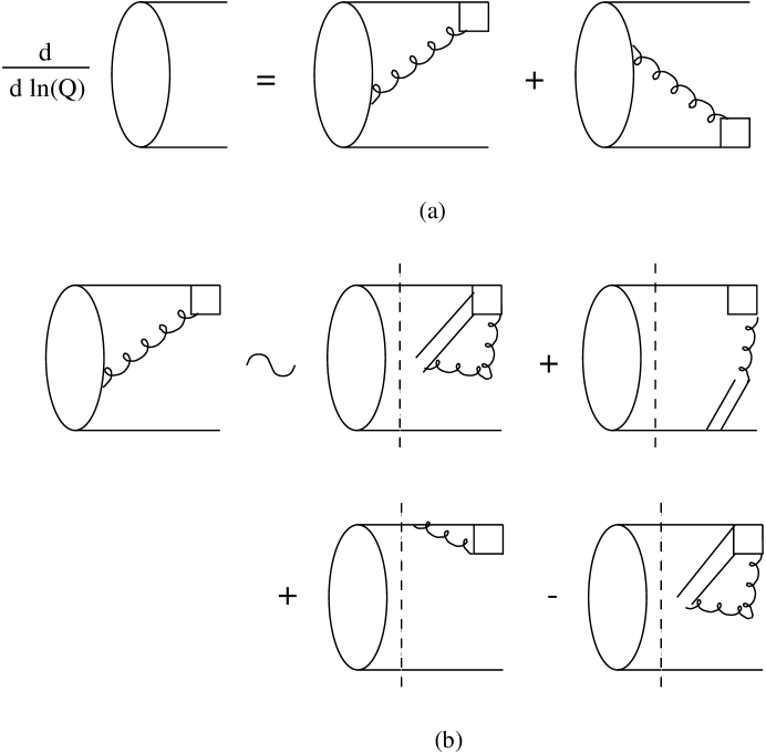
Figure 3: (a) The derivative $d{\cal P}/d\ln Q$ in the axial gauge. (b) The $O(\alpha_{s})$ functions $K$ and $G$.

$T^{a}$ being a color matrix. This new vertex can be easily read off from the combination of Eqs. (12) and (13). After adding together all the diagrams with “differentiated” gluons and using the Ward identity, we arrive at the differential equation of ${\cal P}$ shown in Fig. 3(a), in which the new vertex is represented by a square. An important feature of the new vertex is that the gluon momentum $l$ does not lead to collinear divergences because of the nonvanishing $n^{2}$. The leading regions of $l$ are then soft and ultraviolet, in which Fig. 3(a) can be factorized according to Fig. 3(b) at lowest order. The part on the left-hand side of the dashed line is exactly ${\cal P}$, and that on the right-hand side is assigned to the coefficient function $C$.

Hence, we introduce a function ${\cal K}$ to absorb the soft divergences from the first two diagrams in Fig. 3(b), and a function ${\cal G}$ to absorb the ultraviolet divergences from the other two diagrams. The soft subtraction employed in ${\cal G}$ ensures that the involved momentum flow is hard. Generalizing the two functions to all orders, we derive the differential equation of ${\cal P}$,

$$\frac{d}{d\ln Q}{\cal P}(x,b,P,\mu) = \left[\,2{\cal K}(b\mu)+{\cal G}(x\nu/\mu)+{\cal G}((1-x)\nu/\mu)\right]$$ (15)

$$\times{\cal P}(x,b,P,\mu)\;.$$

${\cal K}$ and ${\cal G}$ have been calculated to one loop, and their single logarithms have been organized to give the evolutions in $b$ and $Q$, respectively [10]. They have ultraviolet poles individually, but their sum ${\cal K}+{\cal G}$ is finite.

Substituting the expressions for ${\cal K}$ and ${\cal G}$ into Eq. (15), we obtain the solution

$${\cal P}(x,b,P,\mu)=\exp\left[-s(xQ,1/b)-s((1-x)Q,1/b)\right]{\bar{\cal P}}(x,b,\mu)\;.$$ (16)

The exponent $s(\xi Q,1/b)$ for $\xi=x$ and $1-x$ is written as [10]

$$s(\xi Q,1/b)=\int_{1/b}^{\xi Q/\sqrt{2}}\frac{dp}{p}\left[\ln\left(\frac{\xi Q}{\sqrt{2}p}\right)A(\alpha_{s}(p))+B(\alpha_{s}(p))\right]\;,$$ (17)

where the anomalous dimensions $A$ to two loops and $B$ to one loop are given by

$$A = {\cal C}_{F}\frac{\alpha_{s}}{\pi}+\left[\frac{67}{9}-\frac{\pi^{2}}{3}-\frac{10}{27}n_{f}+\frac{8}{3}\beta_{0}\ln\left(\frac{e^{\gamma_{E}}}{2}\right)\right]\left(\frac{\alpha_{s}}{\pi}\right)^{2}\;,$$

$$B = \frac{2}{3}\frac{\alpha_{s}}{\pi}\ln\left(\frac{e^{2\gamma_{E}-1}}{2}\right)\;,$$ (18)

with $\gamma_{E}$ the Euler constant. The two-loop expression of the running coupling constant,

$$\frac{\alpha_{s}(\mu)}{\pi}=\frac{1}{\beta_{0}\ln(\mu^{2}/\Lambda^{2})}-\frac{\beta_{1}}{\beta_{0}^{3}}\frac{\ln\ln(\mu^{2}/\Lambda^{2})}{\ln^{2}(\mu^{2}/\Lambda^{2})}\;,$$ (19)

will be substituted into Eq. (17), with the coefficients

$$\beta_{0}=\frac{33-2n_{f}}{12}\;,\;\;\;\beta_{1}=\frac{153-19n_{f}}{24}\;.$$ (20)

To derive Eq. (17), a space-like gauge vector $n\propto(1,-1,{\bf 0})$ has been chosen. We require the ordering of the relevant scales to be $\xi Q>1/b>\Lambda$ as indicated by the integration of $p$ from $1/b$ to $\xi Q$ in Eq. (17). The QCD dynamics below $1/b$ is regarded as being nonperturbative, and absorbed into the initial condition ${\bar{\cal P}}(\xi,b,\mu)$.

4 The Perturbative Pion Form Factor

In this section we evaluate the pion form factor in the framework developed above. Compared to the analysis in [11], the more complete Sudakov factor derived from the two-loop running coupling constant $\alpha_{s}$ in Eq. (19) will be employed and the evolution of the pion wave function will be taken into account. The above resummed PQCD formalism has been widely applied to various exclusive processes, such as the time-like pion form factor [34], proton-antiproton annihilation [35] and proton-proton Landshoff scatterings [36].

4.1 Evolution in $b$

We continue the organization of the large logarithms contained in the factorization formula for the pion form factor in Eq. (9). The functions ${\bar{\cal P}}$ and $\tilde{H}$ still contain single logarithms coming from ultraviolet divergences, which need to be summed using the RG equations [10],

$${\cal D}{\bar{\cal P}}(x,b,\mu)=-2\gamma_{q}{\bar{\cal P}}(x,b,\mu)$$ (21)

$${\cal D}{\tilde{H}}(x_{i},b,Q,\mu)=4\gamma_{q}{\tilde{H}}(x_{i},b,Q,\mu)\;,$$ (22)

with

$${\cal D}=\mu\frac{\partial}{\partial\mu}+\beta(g)\frac{\partial}{\partial g}\;,$$ (23)

and $\gamma_{q}=-\alpha_{s}/\pi$ being the quark anomalous dimension in the axial gauge. Solving Eq. (21), the large-$b$ behavior of $\cal P$ is summarized as

$${\cal P}(x,b,P,\mu) = \exp\left[-s(xQ,1/b)-s((1-x)Q,1/b)-2\int_{1/b}^{\mu}\frac{d\bar{\mu}}{\bar{\mu}}\gamma_{q}(\alpha_{s}(\bar{\mu}))\right]$$ (24)

$$\times{\bar{\cal P}}(x,b,1/b)\;,$$

where the arguments $b$ and $1/b$ of the initial condition ${\bar{\cal P}}$ denote the intrinsic and perturbative $b$ evolutions, respectively. Below we shall ignore the intrinsic $b$ dependence, and assume that ${\bar{\cal P}}=\phi(x,1/b)$.

The RG solution of Eq. (22) is given by

$${\tilde{H}}(x_{i},b,Q,\mu)=\exp\left[-4\,\int_{\mu}^{t}\frac{d\bar{\mu}}{\bar{\mu}}\gamma_{q}(\alpha_{s}(\bar{\mu}))\right]{\tilde{H}}(x_{i},b,Q,t)\;,$$ (25)

where $t$ is the largest mass scale involved in the hard scattering,

$$t=\max(\sqrt{x_{1}x_{2}}Q,1/b)\;.$$ (26)

The scale $\sqrt{x_{1}x_{2}}Q$ is associated with the longitudinal momentum of the hard gluon and $1/b$ with the transverse momentum. The anomalous dimensions $\gamma_{q}$ allow us to take into account the strong couplings of quarks when $t$ is small. With the large logarithms organized, the initial condition ${\tilde{H}}(x_{i},b,Q,t)$ can be taken to coincide with its lowest-order expression, obtained by a Fourier transform of the hard scattering amplitude $H$ in momentum space, as derived from Fig. 1(b),

$$H = \frac{16\pi\alpha_{s}{\cal C}_{F}x_{1}Q^{2}}{(x_{1}Q^{2}+{\bf k}_{1T}^{2})(x_{1}x_{2}Q^{2}+({\bf k}_{1T}-{\bf k}_{2T})^{2})}$$ (27)

$$\approx \frac{16\pi\alpha_{s}{\cal C}_{F}}{x_{1}x_{2}Q^{2}+({\bf k}_{1T}-{\bf k}_{2T})^{2}}\;.$$ (28)

We have neglected the transverse momentum in the numerator of the first expression, and neglected, in addition, the transverse momentum carried by the virtual quarks in the denominator of the second expression. These quark propagators are linear rather than quadratic in $x$. Because Eq. (28) depends on the combination of the transverse momenta, the factorization formula for the pion form factor involves only a single-$b$ integral as shown in Eq. (9). Note that Eq. (28) coincides with Eq. (2) at ${\bf k}_{iT}=0$.

Inserting Eqs. (24) and (25) into Eq. (9), it becomes

$$F_{\pi}(Q^{2}) = 16\pi{\cal C}_{F}\int_{0}^{1}dx_{1}dx_{2}\phi(x_{1},1/b)\phi(x_{2},1/b)\int_{0}^{\infty}bdb\alpha_{s}(t)K_{0}(\sqrt{x_{1}x_{2}}Qb)$$ (29)

$$\times\exp[-S(x_{1},x_{2},b,Q)]\;,$$

with the complete Sudakov exponent

$$S(x_{1},x_{2},b,Q)=\sum_{i=1}^{2}\left[s(x_{i}Q,1/b)+s((1-x_{i})Q,1/b)\right]+4\int_{1/b}^{t}\frac{d\bar{\mu}}{\bar{\mu}}\gamma_{q}(\alpha_{s}(\bar{\mu}))\;.$$ (30)

$K_{0}$ is the modified Bessel function of order zero, which is the Fourier transform to $b$ space of the gluon propagator. Equation (29) for the pion form factor, being a physical quantity, is explicitly $\mu$-independent. This is the consequence of the RG analysis in Eqs. (21) and (22), and the advantage of the resummed PQCD formalism.

Another advantage of Eq. (29), compared to Eq. (1), is the extra $b$ dependence. For $x$ close to zero, i.e., $x_{1}x_{2}Q^{2}<1/b^{2}$, the scale of the radiative corrections is dominated by the transverse distance bridged by the exchanged gluon. If this distance is small, radiative corrections with the argument of $\alpha_{s}$ set to $t$ in the hard scattering amplitude will be small, regardless of the values of $x$. Of course, when $b$ is large and $x_{1}x_{2}Q^{2}$ is small, radiative corrections are still large. However, the Sudakov factor $\exp(-S)$, exhibiting a strong fall off at large $b$, vanishes for $b>1/\Lambda$. We expect that, since Eq. (1) is the asymptotic limit of Eq. (29), as $Q$ increases, the $b$ integral will become more and more dominated by the small-$b$ contributions. If the Sudakov suppression is strong enough, such that the main contributions to the factorization formula come from the short-distance region, the perturbative expansion will be rendered relatively self-consistent. Hence, we propose to analyze Eq. (29), not by cutting off the $x$ integrals near their endpoints, but by testing its sensitivity to the large-$b$ region.

The evolution of the wave function $\phi$ with $b$ is written as [38],

$$\phi(x,1/b)=\frac{3f_{\pi}}{\sqrt{2N_{c}}}x(1-x)\left[\sum_{n=0}^{\infty}a_{n}C^{3/2}_{n}(2x-1)\left(\frac{\alpha_{s}(1/b)}{\alpha_{s}(\mu_{0})}\right)^{\gamma_{n}}\right]\;,$$ (31)

with $\mu_{0}\approx 0.5$ GeV. The coefficient $a_{n}$ and the exponent $\gamma_{n}$ are

$$a_{n} = \frac{5(2n+3)}{(n+2)(n+1)}I_{n}\;,$$ (32)

$$\gamma_{n} = \frac{4}{33-2n_{f}}\left[1+4\sum_{k=2}^{n+1}\frac{1}{k}-\frac{2}{(n+1)(n+2)}\right]\;,$$ (33)

with $I_{0}=2/15$, $I_{1}=0$, $I_{2}=8/35$ and $I_{n}=0$ for $n\geq 3$. The relevant Gegenbauer polynomials are

$$C^{3/2}_{0}(x)=1\;,\;\;\;\;C^{3/2}_{2}(x)=\frac{15}{2}\left(x^{2}-\frac{1}{5}\right)\;.$$ (34)

That is, we adopt the pion wave function

$$\phi(x,1/b)=\frac{3f_{\pi}}{\sqrt{2N_{c}}}x(1-x)\left[1+(5(2x-1)^{2}-1)\left(\frac{\alpha_{s}(1/b)}{\alpha_{s}(\mu_{0})}\right)^{\frac{50}{81}}\right]\;.$$ (35)

It is easy to observe that Eq. (35) approaches $\phi^{AS}$ in Eq. (3) as $1/b\to\infty$, and $\phi^{CZ}$ in Eq. (4) as $1/b\to\mu_{0}$. This is the reason $\phi^{AS}$ is an asympotic wave function, while $\phi^{CZ}$ is a preasympotic one.

We are also interested in the full expression of $H$ in Eq. (27), except for the approximate one in Eq. (28). The corresponding factorization formula involves a double-$b$ integral

$$F_{\pi}(Q^{2}) = 16\pi{\cal C}_{F}\int_{0}^{1}dx_{1}dx_{2}\int_{0}^{\infty}b_{1}db_{1}b_{2}db_{2}\phi(x_{1},1/b_{1})\phi(x_{2},1/b_{2})$$ (36)

$$\times\alpha_{s}(t)K_{0}(\sqrt{x_{1}x_{2}}Qb_{1})\exp\left[-S(x_{1},x_{2},b_{1},b_{2},Q)\right]$$

$$\times\left[\theta(b_{1}-b_{2})K_{0}(\sqrt{x_{1}}Qb_{1})I_{0}(\sqrt{x_{1}}Qb_{2})\right.+$$

$$\left.\theta(b_{2}-b_{1})K_{0}(\sqrt{x_{1}}Qb_{2})I_{0}(\sqrt{x_{1}}Qb_{1})\right]\;,$$

with the Sudakov exponent

$$S = \sum_{i=1}^{2}\left[s(x_{i}Q,1/b_{i})+s((1-x_{i})Q,1/b_{i})\right]$$ (37)

$$+2\int_{1/b_{1}}^{t}\frac{d\bar{\mu}}{\bar{\mu}}\gamma_{q}(\alpha_{s}(\bar{\mu}))+2\int_{1/b_{2}}^{t}\frac{d\bar{\mu}}{\bar{\mu}}\gamma_{q}(\alpha_{s}(\bar{\mu}))\;,$$

and the hard scale

$$t={\rm max}\left[\sqrt{x_{1}x_{2}}Q,1/b_{1},1/b_{2}\right]\;.$$ (38)

4.2 Numerical Results

Results on the behaviour of the Sudakov suppression in the large $b$ region where presented in [11]. There is no suppression for small $b$, where the two fermion lines are close to each other. In this region the higher-order corrections should be absorbed into the hard amplitude, instead of being adsorbed into the pion wave function. Hence, we set any factor $\exp[-s(\xi Q,1/b)]$ to unity for $\xi Q/\sqrt{2}<1/b$. Similarly, we also set the complete Sudakov exponential $\exp(-S)$ in Eq. (29) to unity, whenever it exceeds unity in the small-$b$ region. As $b$ increases, $\exp(-S)$ decreases, reaching zero at $b=1/\Lambda$. Suppression in the large $b$ region is stronger for larger $Q$.

We choose the QCD scale $\Lambda=0.15$ GeV for the numerical analysis of the pion form factor below. It can be shown that the results will differ only by 10%, if $\Lambda=0.1$ GeV or $\Lambda=0.2$ GeV is adopted.

In order to see how the contributions to Eq. (29) are distributed in the $b$ space under Sudakov suppression, the integration is done with $b$ cut off at $b_{c}$. Typical numerical results are displayed in Fig. 4 for the use of $\phi$ in Eq. (35). The curves, showing the dependence of $Q^{2}F_{\pi}$ on $b_{c}$, rise from zero at $b_{c}=0$, and reach their full height at $b_{c}=1/\Lambda$, beyond which any remaining contributions are regarded as being truly nonperturbative. To be quantitive, we determine a cutoff up to which half of the whole contribution has been accumulated. For $Q^{2}=4$ and 9 GeV², 50% of $Q^{2}F_{\pi}$ comes from the regions with $b\leq 3.6$ GeV^-1 [$\alpha_{s}(1/b)/\pi\leq 0.32$] and with $b\leq 3.0$ GeV^-1 [$\alpha_{s}(1/b)/\pi\leq 0.21$], respectively. A liberal standard to judge the self-consistency of the perturbative method would be that half of the results arise from the region where $\alpha_{s}(1/b)/\pi$ is not larger than, say, 0.5. From this point of view, PQCD becomes self-consistent at about $Q^{2}\sim 4$ GeV². This conclusion is similar to that drawn in [11], where $\phi^{CZ}$ and $\phi^{AS}$ were employed. As anticipated, the perturbative calculation improves with an increase of the momentum transfer.

Results of $Q^{2}F_{\pi}$ from $\phi^{AS}$, $\phi^{CZ}$ and $\phi$ in Eq. (35), as well as the experimental data [21, 22, 23, 24], are shown in Fig. 5. The curve corresponding to Eq. (35) is located beyond the one corresponding to $\phi^{CZ}$ (and beyond the one corresponding to $\phi^{AS}$, of course), indicating that the evolution of the pion wave function, especially the portion from $1/b<\mu_{0}$, plays an essential role. Our predictions for $Q^{2}>2$ GeV² are in a good agreement with the data. For $Q^{2}<2$ GeV², the curve deviates from the data, implying the dominance of the nonperturbative contrubution. However, we emphasize that the wave function $\phi(x,1/b)$, regarded as an expansion in $\alpha_{s}(1/b)/\alpha_{s}(\mu_{0})$, becomes meaningless gradually as $1/b\to\Lambda<\mu_{0}$. Hence, we shall not claim that the match of our results with the data is conclusive. It is possible that higher-twist contributions from other Fock states are important as argued in [39]. Nonetheless, the resummed PQCD predictions are indeed reliable at least near the high end of the accessible energy range, where the curve from $\phi$ approaches that from $\phi^{CZ}$.

At last, we evaluate the pion form factor using the double-$b$ factorization formula in Eq. (36), and the results are presented in Fig. 6. Those derived from the single-$b$ formula in Eq. (29) and the experimental data are also displayed for comparison. It is found that the two curves are consistent with each other especially in the region with $Q^{2}\sim 5$-10 GeV². The consistency hints that the approximation of neglecting the transverse momenta carried by the virtual quarks makes sense. Therefore, we shall employ the same approximation in order to simplify the multidimensional integrals, when evaluating the hard scattering amplitudes for the proton form factor.

We have stated that the function ${\bar{\cal P}}(x,b,1/b)$ in Eq. (24) contains the intrinsic $b$ dependence denoted by its argument $b$, except for the perturbative evolution with $b$ shown in Eq. (35). This intrinsic dependence, providing further suppression at large $b$, has been discussed in detail in [40]. Since it depends on the parametrization, we shall not consider it here.

5 The Perturbative Proton Form Factor

With the success of the resummed PQCD formalism in the study of the pion form factor, we are encouraged to apply it to the proton form factor. We concentrate on the proton Dirac form factor $F_{1}^{p}$, which has been widely calculated based on the standard PQCD theory [8, 18, 26, 27, 33, 41, 42, 43, 44]. Another form factor $F_{2}(Q^{2})\sim O(1/Q^{6})$ is much smaller than $F_{1}(Q^{2})\sim O(1/Q^{4})$ in the asymptotic region [25]. It has been shown that the asymptotic proton wave function $\phi(x_{i})\propto x_{1}x_{2}x_{3}$ fails to give the correct sign for $F_{1}^{p}$, and generates much smaller values than the experimental data [41, 44]. Highly asymmetric distribution amplitudes, such as the Chernyak-Zhitnitsky (CZ) [25] and King-Sachrajda (KS) [45] wave functions derived from QCD sum rules, reverse the sign and enlarge the magnitude of the predictions. However, it was also critically pointed out that the perturbative calculations based on the above phenomenologically acceptable wave functions are typically dominated by soft virtual gluon exchanges, and violate the assumption that the momentum transfer proceeds perturbatively [8]. We shall show that the resummed PQCD formalism can give reliable predictions which are consistent with the experimental data.

5.1 Factorization Formula

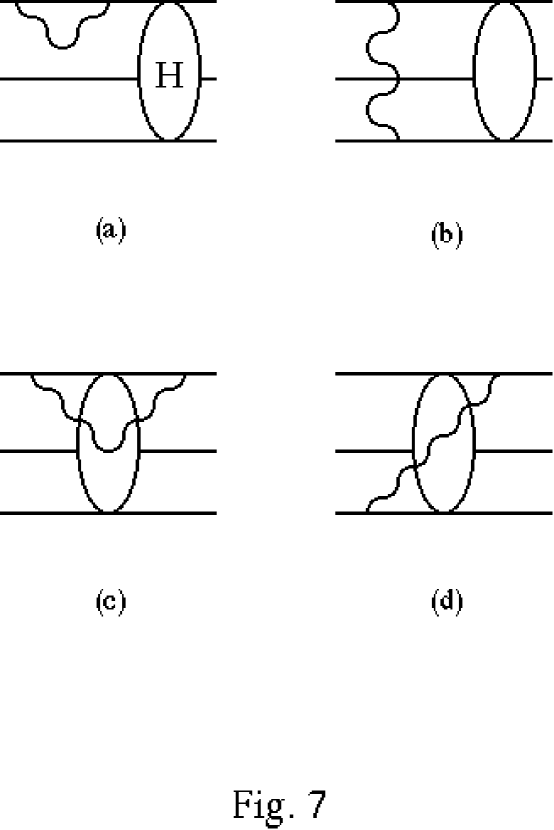
Figure 7: (a)-(d) Radiative corrections to the basic diagrams for the proton Dirac form factor.

As stated in Sect. 3, the factorization formulas for exclusive QCD processes require the investigation of those leading regions in the diagrams describing the radiative corrections where the dominant contributions arise from. Similarly, we work in the axial gauge $n\cdot A=0$ as in the pion case. The two-particle reducible diagrams, like Figs. 7(a) and 7(b), which are dominated by the collinear divergences, are grouped into the distribution amplitudes, and generate their Sudakov evolution. The bubbles may be regarded as the basic photon-quark scattering diagrams. The two-particle irreducible diagrams Figs. 7(c) and 7(d) contain only soft divergences, which cancel asymptotically. These types of corrections are then dominated by momenta of order $Q^{2}$, and absorbed into the hard scattering amplitude $H$. Hence, the factorization formula for the proton Dirac form factor includes three factors [46]

$$F_{1}^{p}(Q^{2}) = \int_{0}^{1}(dx)(dx^{\prime})(d{\bf k}_{T})(d{\bf k}^{\prime}_{T})\bar{Y}_{\alpha^{\prime}\beta^{\prime}\gamma^{\prime}}(k_{i}^{\prime},P^{\prime},\mu)$$ (39)

$$\times H_{\alpha^{\prime}\beta^{\prime}\gamma^{\prime}\alpha\beta\gamma}(k_{i},k^{\prime}_{i},Q,\mu)Y_{\alpha\beta\gamma}(k_{i},P,\mu)\;,$$

with $P=(P^{+},0,{\bf 0})$ the initial-state proton momentum, and

$$(dx) = dx_{1}dx_{2}dx_{3}\delta(\sum_{i=1}^{3}x_{i}-1)\;,$$

$$(d{\bf k}_{T}) = d^{2}{\bf k}_{1T}d^{2}{\bf k}_{2T}d^{2}{\bf k}_{3T}\delta(\sum_{i=1}^{3}{\bf k}_{iT})\;.$$ (40)

$x_{i}=k_{i}^{+}/P^{+}$ and ${\bf k}_{iT}$ are the longitudinal momentum fractions and transverse momenta of the parton $i$, respectively. The primed variables $P^{\prime}=(0,P^{{}^{\prime}-},{\bf 0})$ and $x^{\prime}_{i}=k_{i}^{{}^{\prime}-}/P^{{}^{\prime}-}$ are associated with the final-state proton. $Q^{2}=2P\cdot P^{\prime}$ is the momumtum transfer, and the scale $\mu$ is the renormalization and factorization scale. In the Breit frame we have $P^{+}=P^{{}^{\prime}-}=Q/\sqrt{2}$. Similarly, we have taken into account the transverse degrees of freedom of a parton as indicated in Eq. (39). If the end-point regions are not important, one may drop the $k_{T}$ dependence in the hard scattering $H$, and integrate out $k_{T}$ in the proton distribution amplitude $Y$, arriving at the standard factorization formula.

The initial distribution amplitude $Y_{\alpha\beta\gamma}$, defined by the matrix element of three local operators in the axial gauge, is written as [10, 25],

$$Y_{\alpha\beta\gamma} = \frac{1}{2\sqrt{2}N_{c}}\int\prod_{l=1}^{2}\frac{dy_{l}^{-}d{\bf y}_{l}}{(2\pi)^{3}}e^{\textstyle ik_{l}\cdot y_{l}}\epsilon^{abc}\langle 0|T[u_{\alpha}^{a}(y_{1})u_{\beta}^{b}(y_{2})d_{\gamma}^{c}(0)]|P\rangle$$ (41)

$$= \frac{f_{N}(\mu)}{8\sqrt{2}N_{c}}[(\,/\hbox to0.0pt{\hss P}C)_{\alpha\beta}(\gamma_{5}N)_{\gamma}V(k_{i},P,\mu)+(\,/\hbox to0.0pt{\hss P}\gamma_{5}C)_{\alpha\beta}N_{\gamma}A(k_{i},P,\mu)$$

$$\mbox{ }-(\sigma_{\mu\nu}P^{\nu}C)_{\alpha\beta}(\gamma^{\mu}\gamma_{5}N)_{\gamma}T(k_{i},P,\mu)]\;,$$

where $|P\rangle$ is the initial proton state, $u$ and $d$ the quark fields, $a$, $b$ and $c$ the color indices, and $\alpha$, $\beta$ and $\gamma$ the spinor indices. In our notation, 1,2 label the two $u$ quarks and 3 labels the $d$ quark. The second form, showing the explicit Dirac matrix structure, is obtained from the spin property of quark fields [25], where $N$ is the proton spinor, $C$ the charge conjugation matrix and $\sigma_{\mu\nu}\equiv[\gamma_{\mu},\gamma_{\nu}]/2$. The dimensional constant $f_{N}$ is determined by the normalization of the distribution amplitude [47]. The amplitude $\bar{Y}_{\alpha^{\prime}\beta^{\prime}\gamma^{\prime}}(k_{i}^{\prime},P^{\prime},\mu)$ for the final-state proton is defined similarly. The permutation symmetry between the two $u$ quarks gives the relations among the wave functions [25]

$$V(k_{1},k_{2},k_{3},P,\mu)=V(k_{2},k_{1},k_{3},P,\mu)\;,$$

$$A(k_{1},k_{2},k_{3},P,\mu)=-A(k_{2},k_{1},k_{3},P,\mu)\;,$$

$$T(k_{1},k_{2},k_{3},P,\mu)=T(k_{2},k_{1},k_{3},P,\mu)\;.$$ (42)

Since the total isospin of the three quarks is equal to $1/2$, we have [25]

$$2T(k_{1},k_{2},k_{3},P,\mu)=\psi(k_{1},k_{3},k_{2},P,\mu)+\psi(k_{2},k_{3},k_{1},P,\mu)\;,$$ (43)

with

$$\psi(k_{1},k_{2},k_{3},P,\mu)=V(k_{1},k_{2},k_{3},P,\mu)-A(k_{1},k_{2},k_{3},P,\mu)\;.$$ (44)

The combination of Eqs. (42) and (43) leads to

$$V(k_{1},k_{2},k_{3},P,\mu)=\frac{1}{2}\;\left[\psi(k_{2},k_{1},k_{3},P,\mu)+\psi(k_{1},k_{2},k_{3},P,\mu)\right]$$

$$A(k_{1},k_{2},k_{3},P,\mu)=\frac{1}{2}\;\left[\psi(k_{2},k_{1},k_{3},P,\mu)-\psi(k_{1},k_{2},k_{3},P,\mu)\right]\;.$$ (45)

Hence, the factorization formula in fact involves only one independent wave function $\psi$.

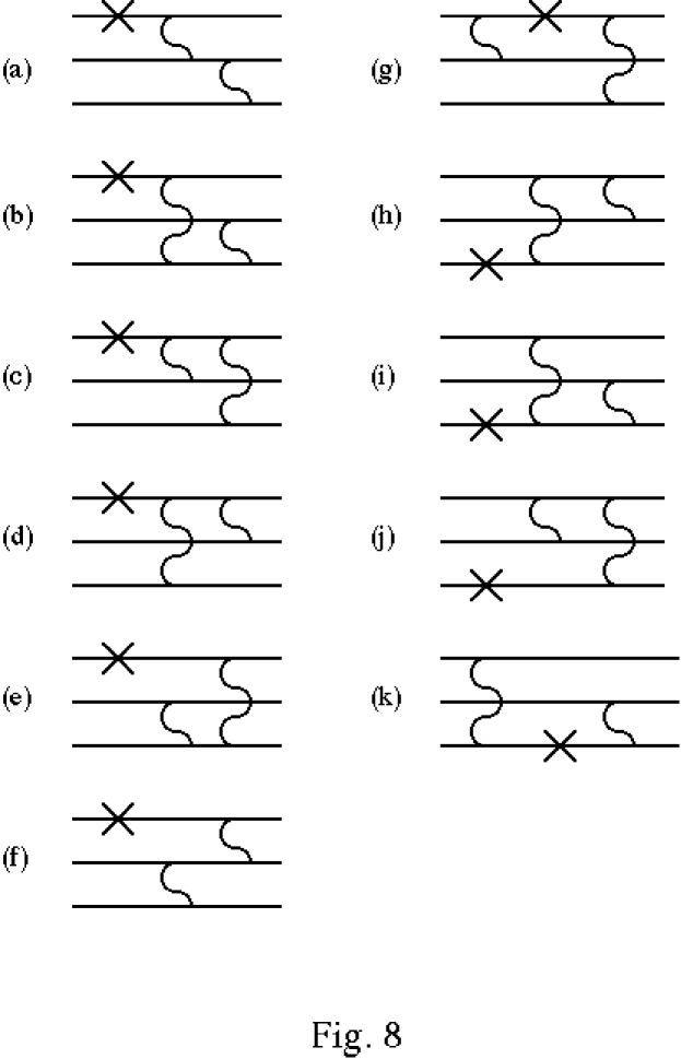
Figure 8: Independent lowest-order hard scattering subdiagrams for the proton Dirac form factor. The bottom line represents the $d$ quark.

The hard-scattering kernel $H_{\alpha^{\prime}\beta^{\prime}\gamma^{\prime}\alpha\beta\gamma}$ can be calculated perturbatively. To lowest order in $\alpha_{s}$ with two hard exchanged gluons, 42 diagrams are drawn for the proton form factor. This number is reduced to 21 when the permutation symmetry between the incoming and outgoing protons is considered. These 21 diagrams are further divided into two categories, which transform into one anoother by an interchange of the two $u$ quarks, so that it is enough to calculate only 11 of them, as shown in Fig. 8. The explicit expression of the integrand $\bar{Y}_{\alpha^{\prime}\beta^{\prime}\gamma^{\prime}}H_{\alpha^{\prime}\beta^{\prime}\gamma^{\prime}\alpha\beta\gamma}Y_{\alpha\beta\gamma}$, corresponding to each diagram in Fig. 8, is listed in Table 1. For more details we refer to [46]. The diagrams with three-gluon vertices vanish at leading twist and are thus ignored.

Applying a series of variable changes [46], the summation of the contributions over the 42 diagrams is reduced to only two terms. Equation (39) becomes

$$F_{1}^{p}(Q^{2}) = \frac{8\pi^{2}}{27}\int_{0}^{1}(dx)(dx^{\prime})(d{\bf k}_{T})(d{\bf k}^{\prime}_{T})[f_{N}(\mu)]^{2}$$ (46)

$$\times \sum_{j=1}^{2}\,H_{j}(k_{i},k^{\prime}_{i},Q,\mu)\,\Psi_{j}(k_{i},k^{\prime}_{i},P,P^{\prime},\mu)\;.$$

with

$$H_{1}=\frac{2\alpha_{s}^{2}(\mu)}{3[(1-x_{1})(1-x_{1}^{\prime})Q^{2}+({\bf k}_{1T}-{\bf k}^{\prime}_{1T})^{2}][x_{2}x_{2}^{\prime}Q^{2}+({\bf k}_{2T}-{\bf k}^{\prime}_{2T})^{2}]}\;,$$

$$H_{2}=\frac{2\alpha_{s}^{2}(\mu)}{3[x_{1}x_{1}^{\prime}Q^{2}+({\bf k}_{1T}-{\bf k}^{\prime}_{1T})^{2}][x_{2}x_{2}^{\prime}Q^{2}+({\bf k}_{2T}-{\bf k}^{\prime}_{2T})^{2}]}\;,$$ (47)

and

$$\Psi_{1}=\frac{2(\psi\psi^{\prime})_{123}+8(TT^{\prime})_{123}+2(\psi\psi^{\prime})_{132}+8(TT^{\prime})_{132}-(\psi\psi^{\prime})_{321}-(\psi\psi^{\prime})_{231}}{(1-x_{1})(1-x_{1}^{\prime})}\;,$$

$$\Psi_{2}=\frac{2(\psi\psi^{\prime})_{132}-2(TT^{\prime})_{123}}{(1-x_{2})(1-x_{1}^{\prime})}+\frac{(\psi\psi^{\prime})_{123}-8(TT^{\prime})_{132}-2(\psi\psi^{\prime})_{321}}{(1-x_{3})(1-x_{1}^{\prime})}\;.$$ (48)

The notation $(\psi\psi^{\prime})_{123}$ represents

$$(\psi\psi^{\prime})_{123}=\psi(k_{1},k_{2},k_{3},P,\mu)\psi(k_{1}^{\prime},k_{2}^{\prime},k_{3}^{\prime},P^{\prime},\mu)\;,$$ (49)

and $(TT^{\prime})_{123}$ is defined in a similar way and we have inserted the electric charges of the quarks. The transverse momenta carried by the virtual quarks in the hard scattering subdiagram have been neglected for simplicity as indicated in Eq. (47). This approximation equates the initial and final transverse distances among all pairs of valence quarks. At the same time, fermion energies such as $x_{i}Q^{2}$ will not be among the characteristic scales of the hard scattering, and the evolution of $H$ in $Q$ will be simpler. The accuracy of this approximation has been roughly discussed in Sect. 4.

5.2 Sudakov Suppression

Reexpressing Eq. (46) in the Fourier transform space, we obtain

$$F_{1}^{p}(Q^{2}) = \sum_{j=1}^{2}\frac{8\pi^{2}}{27}\int_{0}^{1}(dx)(dx^{\prime})(d{\bf b})[f_{N}(\mu)]^{2}$$ (50)

$$\times{\tilde{H}}_{j}(x_{i},x^{\prime}_{i},{\bf b}_{i},Q,\mu)\Psi_{j}(x_{i},x^{\prime}_{i},{\bf b}_{i},P,P^{\prime},\mu)\;,$$

with ${\bf b}_{i}$ the conjugate variables to ${\bf k}_{iT}$, and $(d{\bf b})=d^{2}{\bf b}_{1}d^{2}{\bf b}_{2}/(2\pi)^{4}$. The above factorization formula involves only the integration over ${\bf b}$ (not ${\bf b}^{\prime}$) as stated above. The Sudakov resummation of the large logarithms in the Fourier transformed wave function ${\cal P}$ leads to

$${\cal P}(x_{i},{\bf b}_{i},P,\mu) = \exp\left[-\sum_{l=1}^{3}s(x_{l}Q,w)-3\int_{w}^{\mu}\frac{d\bar{\mu}}{\bar{\mu}}\gamma_{q}\left(\alpha_{s}(\bar{\mu})\right)\right]$$ (51)

$$\times\phi(x_{i},w)\;,$$

with the scale

$$w=\min(1/b_{1},1/b_{2},1/b_{3})\;,$$ (52)

and $b_{3}=|{\bf b}_{1}-{\bf b}_{2}|$. The function $\phi$, obtained by factoring the $Q$ dependence out of ${\cal P}$, corresponds to the naive parton model. Again, we have dropped the intrinsic $b$ dependence of the proton wave function. The exponent $s(xQ,w)$ has been given in Eq. (17).

Note the choice of the infrared cutoff in Eq. (52), which differs from that adopted in the previous analysis [46], but the same as $w=1/\max(b_{1},b_{2},b_{3})$ in [48]. In [46] the different transverse separations were assigned to each exponent $s$ and to each integral involving $\gamma_{q}$:

$${\cal P}(x_{i},{\bf b}_{i},P,\mu) = \exp\left[-\sum_{l=1}^{3}\left(s(x_{l}Q,1/b_{l})+\int_{1/b_{l}}^{\mu}\frac{d\bar{\mu}}{\bar{\mu}}\gamma_{q}\left(\alpha_{s}(\bar{\mu})\right)\right)\right]$$ (53)

$$\times\phi(x_{i},w)\;.$$

The Sudakov factor in Eq. (53) does not suppress the soft divergences coming from $b_{l}\to 1/\Lambda$ completely. For example, the divergences from $b_{1}\to 1/\Lambda$, which appear in the integral involving $\gamma_{q}$ and in $\phi(x_{i},w)$ at $w\to\Lambda$, survive as $x_{1}\to 0$, since $s(x_{1}Q,1/b_{1})$ vanishes, while $s(x_{2}Q,1/b_{2})$ and $s(x_{3}Q,1/b_{3})$ may remain finite. On the other hand, $w$ should play the role of the factorization scale, above which QCD corrections give the perturbative evolution of ${\cal P}$ shown in Eq. (51), and below which they are absorbed into the nonperturbative initial condition $\phi$. Hence, it is not appropriate to choose the infrared cutoff of the Sudakov evolution different from $w$. An alternative choice of the scale [35],

$$w^{\prime}=\max(1/b_{1},1/b_{2},1/b_{3})\;,$$ (54)

also removes the soft divergences. We argue that the factorization scale should be chosen to diminish the largest logarithms contained in $\phi$, which are proportional to $\ln(\mu/w)$. However, $w^{\prime}$ does not serve this purpose. In the numerical analysis below we shall truncate the integrations over $b_{1}$ and $b_{2}$, in order to examine how much contributions are accumulated in the short-distance (perturbative) region. Since small values of $b_{1}$ and $b_{2}$ do not guarantee a small $b_{3}$ due to the vector sum, we shall require $1/b_{3}$ to be greater than $\Lambda$, such that the running coupling constant $\alpha_{s}(w)$ is well defined.

The evolution of the hard scattering amplitudes is written as

$${\tilde{H}}_{j}(x_{i},x_{i}^{\prime},{\bf b}_{i},Q,\mu) = \exp\left[-3\sum_{l=1}^{2}\int^{t_{jl}}_{\mu}\frac{d\bar{\mu}}{\bar{\mu}}\,\gamma_{q}\left(\alpha_{s}(\bar{\mu})\right)\right]$$ (55)

$$\times{\tilde{H}}_{j}(x_{i},x_{i}^{\prime},{\bf b}_{i},Q,t_{j1},t_{j2})\;,$$

with

$$t_{11}=\max\left[\sqrt{(1-x_{1})(1-x_{1}^{\prime})}Q,1/b_{1}\right]\;,$$

$$t_{21}=\max\left[\sqrt{x_{1}x_{1}^{\prime}}Q,1/b_{1}\right]\;,$$

$$t_{12}=t_{22}=\max\left[\sqrt{x_{2}x_{2}^{\prime}}Q,1/b_{2}\right]\;.$$ (56)

The first scales in the brackets are associated with the longitudinal momenta of the hard gluons and the second with the transverse momenta. The arguments $t_{j1}$ and $t_{j2}$ of ${\tilde{H}}_{j}$ mean that each $\alpha_{s}$ is evaluated at the largest mass scale of the corresponding hard gluon.

Inserting Eqs. (51) and (55) into (50), we obtain

$$F_{1}^{p}(Q^{2}) = \sum_{j=1}^{2}\frac{4\pi}{27}\int_{0}^{1}(dx)(dx^{\prime})\int_{0}^{\infty}b_{1}db_{1}b_{2}db_{2}\int_{0}^{2\pi}d\theta[f_{N}(w)]^{2}$$ (57)

$$\times{\tilde{H}}_{j}(x_{i},x_{i}^{\prime},b_{i},Q,t_{j1},t_{j2})\,\Psi_{j}(x_{i},x^{\prime}_{i},w)$$

$$\times\exp\left[-S(x_{i},x_{i}^{\prime},w,Q,t_{j1},t_{j2})\right]\;,$$

where

$${\tilde{H}}_{1}=\frac{2}{3}\alpha_{s}(t_{11})\alpha_{s}(t_{12})K_{0}\left(\sqrt{(1-x_{1})(1-x_{1}^{\prime})}Qb_{1}\right)K_{0}\left(\sqrt{x_{2}x_{2}^{\prime}}Qb_{2}\right)$$

$${\tilde{H}}_{2}=\frac{2}{3}\alpha_{s}(t_{21})\alpha_{s}(t_{22})K_{0}\left(\sqrt{x_{1}x_{1}^{\prime}}Qb_{1}\right)K_{0}\left(\sqrt{x_{2}x_{2}^{\prime}}Qb_{2}\right)$$

are derived from the Fourier transform of Eq. (47), and the expressions for $\Psi_{j}$ are the same as those in Eq. (48) but with $\psi(k_{i},P,\mu)$ replaced by $\phi(x_{i},w)$. The variable $\theta$ is the angle between ${\bf b}_{1}$ and ${\bf b}_{2}$. The Sudakov exponent $S$ is written as

$$S(x_{i},x^{\prime}_{i},w,Q,t_{j1},t_{j2}) = \sum_{l=1}^{3}s(x_{l}Q,w)+3\int_{w}^{t_{j1}}\frac{d\bar{\mu}}{\bar{\mu}}\gamma_{q}\left(\alpha_{s}(\bar{\mu})\right)$$ (58)

$$+\sum_{l=1}^{3}s(x^{\prime}_{l}Q,w)+3\int_{w}^{t_{j2}}\frac{d\bar{\mu}}{\bar{\mu}}\gamma_{q}\left(\alpha_{s}(\bar{\mu})\right)\;.$$

Similarly, the two-loop running coupling constant $\alpha_{s}$ in Eq. (19) is employed to derive the complete Sudakov factor. This is an improvement of the analyses in [46, 48].

The evolution of $f_{N}$ is given by

$$f_{N}(w)=f_{N}(\mu_{0})\left[\frac{\alpha_{s}(w)}{\alpha_{s}(\mu_{0})}\right]^{1/(6\beta_{0})}\;,$$ (59)

with $\mu_{0}\approx 1$ GeV and the initial condition $f_{N}(\mu_{0})=(5.2\pm 0.3)\times 10^{-3}$ GeV² [25]. For the wave function $\phi$, we consider both the CZ model [25] and KS model [45]. They are decomposed into

$$\phi(x_{i},w)=\phi^{AS}(x_{i})\sum_{j=0}^{5}N_{j}\left[\frac{\alpha_{s}(w)}{\alpha_{s}(\mu_{0})}\right]^{b_{j}/(4\beta_{0})}a_{j}A_{j}(x_{i})\;,$$ (60)

where the constants $N_{j}$, $a_{j}$ and $b_{j}$, and the first six Appel polynomials $A_{j}(x_{i})$ [18, 42] are listed in Table 2. The function $\phi^{AS}(x_{i})=120x_{1}x_{2}x_{3}$ is the asymptotic form of $\phi$ mentioned before.

5.3 Numerical Results

If we employ the Sudakov exponent in Eq. (58) directly, we obtain the results $Q^{4}F_{1}^{p}=0.55$ GeV⁴ for $Q^{2}=10$ GeV² and $Q^{4}F_{1}^{p}=0.48$ GeV⁴ for $Q^{2}=40$ GeV² by using the KS wave function, which are only about half of the experimental data. These values are close to those derived in [48]. However, we argue that there is a freedom to choose the scales for the Sudakov evolution [10]. For example, the ultraviolet cutoff $c\xi Q/\sqrt{2}$ for the integral in Eq. (17), with $c$ a constant of order unity, is as appropriate as $\xi Q/\sqrt{2}$. Hence, we may determine $c$ by fitting the predictions for the pion form factor to the data $Q^{2}F_{\pi}\approx 0.35$ GeV² for $Q^{2}\sim 5$-10 GeV², and apply it to the evaluation of the proton form factor. This procedure leads to $c\approx 0.6$. The change from $c=1.0$ to $c=0.6$ enhances the results of the pion form factor by about 15%. We expect that this change in $c$ will give a larger enhancement in the proton case, since the proton form factor is more sensitive to the evolution scales. We emphasize that the parameter $c=0.6$ is introduced in order to explain the data. It is certainly legitimate to question this smaller value of $c$, and argue that higher Fock state contributions may be important.

In the numerical analysis below we adopt the Sudakov exponent $S(x_{i},x^{\prime}_{i},w,0.6Q,t_{j1},t_{j2})$. We investigate the sensitivity of our predictions to the large $b_{1}$-$b_{2}$ region, choosing $\Lambda=0.2$ GeV. If the perturbative contributions dominate, an essential amount of $Q^{4}F_{1}^{p}$ will be quickly accumulated below a common cutoff $b_{c}$ of $b_{1}$ and $b_{2}$. The numerical outcomes are displayed in Fig. 9. All the curves, showing the dependence of $Q^{4}F_{1}^{p}$ on $b_{c}$, increase from the origin and reach their full height at $b_{c}=1/\Lambda$. A quantitative measure of self-consistency is that half of the contribution to $Q^{4}F_{1}^{p}$ is accumulated in the region characterized by $\alpha_{s}/\pi\leq 0.5$. Based on this standard, the results above $Q^{2}\sim 20$ GeV² are reliable. At a higher energy $Q^{2}=40$ GeV², the contribution from the perturbative region amounts approximately to 65% of the entire contribution. It implies that the applicability of PQCD to the proton form factor at currently accessible energy scale $Q^{2}\sim 30$ GeV² may be justified.

Note that the saturation of the proton form factor in the large $b$ region is slower than that in the pion case, because the Sudakov suppression for the former is more moderate compared to that for the latter. The proton form factor involves more $\gamma_{q}$, which enhance the nonperturbative contributions, and the partons are softer, thereby weakening the Sudakov suppression. The slower transition of the proton form factor to PQCD as $Q^{2}$ increases can also be understood as follows. The hard gluon exchange diagrams give leading contributions of order $(\alpha_{s}/\pi)^{2}$, rather than $\alpha_{s}/\pi$ as in the pion case, so that soft contributions, always suppressed by a power of $M^{2}/Q^{2}$ with $M$ a typical hadronic mass, become relatively stronger [31].

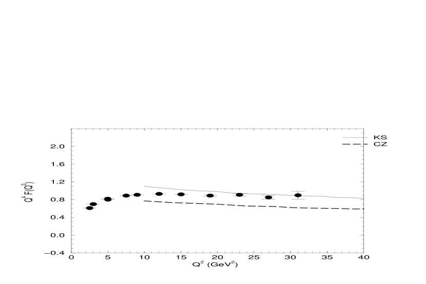
Figure 9: Dependence of $Q^{4}F_{1}^{p}(Q^{2})$ on the cutoff $b_{c}$ from the KS wave function for $Q^{2}=20$ GeV² (dotted line), for $Q^{2}=30$ GeV² (dashed line), and for $Q^{2}=40$ GeV² (solid line).

Figure 10: Dependence of $Q^{4}F_{1}^{p}(Q^{2})$ on $Q^{2}$ from the KS wave function (solid line) and from the CZ wave function (dashed line). The experimental data are also shown.

In Fig. 10 we compare our predictions for $Q^{4}F_{1}^{p}(Q^{2})$ to the experimental data, which are extracted from the data of elastic electron-proton cross section [27, 49]. The match between the curve corresponding to the KS wave function and the data is obvious. Below $Q^{2}\sim 20$ GeV², the deviation of the curve from the data becomes larger. The CZ model generates results which are smaller than those from the KS model by a factor 2/3. The above analysis implies that the KS wave function is more phenomenologically appropriate. We shall adopt this model for the proton wave function in the future studies. The sensitivity of our predictions to the variation of the QCD scale parameter $\Lambda$ is also examined. We find that the decrease of $\Lambda$ to 0.1 GeV enhances $Q^{4}F_{1}^{p}$ by about 10%.

6 Sum Rules for Compton Scattering

In this section we review the derivation of the local duality sum rule for pion Compton scattering. The theoretical motivations and justifications of the validity of sum rules for the invariant amplitudes of RCS or VCS can be found in [4].

As emphasized by Nesterenko and Radyushkin in their work on the sum rule analysis of the pion form factor [16], the dominant contribution to the intermediate energy behaviour of the pion form factor comes from a “soft” diagram, which is nonfactorizable and is interpreted as an overlap of initial and final state wave functions. According to this viewpoint, the inclusion of a hard scattering in the intermediate state, as suggested by the PQCD factorization formalism, does not describe the correct dynamics. There is at the moment no general consensus on this issue, and the experimental input is going to be crucial in order to rule out some of the alternatives.

We remind briefly that the sum rule analysis of VCS requires a detailed study of the properties of analyticity of the diagrams appearing in the Operator Product Expansion of a 4-current correlator, and this task has been performed in detail in [6]. The existence of a finite contour dispersion relation, which allows the application of the usual OPE technique, has also been shown to hold with sufficient accuracy. The sum rules obtained by this method, which are similar to the form factor sum rules, are now characterized by both an “$s$” and a “$t$” dependence, and are shown to hold at a fixed value of the ratio $-t/s$. The basic idea of this approach is to connect the invariant amplitudes of a “true” (i.e., with on-shell pions or protons) scattering to an OPE series, which is expressed in terms of a perturbative “spectral function” and of the corresponding condensates.

We show that the sum rule can be organized in a rather compact form in the Breit frame of the pion, where the spectral density becomes polynomial in a variable called $Q$. In the sum rule description of both form factors and Compton scattering, $Q$ is a function of various kinematic invariants, such as the pion virtualities (here denoted as $s_{1}$, $s_{2}$), plus the usual $s$ and $t$ invariants. In fact, we recall that the OPE side of the sum rule is calculated with off-shell pions, since it has to correspond to a short-distance factorization. This variable $Q$, which parametrizes the large light-cone components of the incoming (or outgoing) hadron in the scattering process, is used to analyze the power suppression of the various contributions to the spectral function. $Q$ is then averaged in the dispersion integral over the virtualities of the hadron momenta.

We also evaluate the power corrections proportional to the quark and gluon condensates, and give the complete expressions of the spectral functions for the helicity amplitudes involved in pion Compton scattering. A new Borel sum rule is derived and compared to the corresponding one for the pion form factor. The Borel transform is defined in its “contour form”, and is used to reduce the “noise” or “background contribution” to the sum rule. Ultimately, the success of any sum rule program relies on the choice of a “good” correlator with minimal noise and maximum projection onto the physical states that we intend to study. Assessing the error in this unobvious re-organization of the perturbative expansion, via the OPE, is nontrivial and requires a case-by-case study. We remind that sum rules are just a different model, closer to a PQCD description, and like all models, should be handled with caution. In some situations they can help us describe the underlying dynamics better than other models, and, as such, can be a very useful tool of analysis.

6.1 Overview of the Method

We start our discussion by quoting the main results of [4]. Consider the following 4-point amplitude as graphically described in Fig. 11,

$$\Gamma_{\nu\lambda\mu\sigma}(p_{1}^{2},p_{2}^{2},s,t) = i\int{\rm d}^{4}x\,{\rm d}^{4}y\,{\rm d}^{4}z\exp(-ip_{1}\cdot x+ip_{2}\cdot y-iq_{1}\cdot z)$$ (61)

$$\times\langle 0|T\left(\eta_{\nu}(y)J_{\lambda}(z)J_{\mu}(0)\eta_{\sigma}^{\dagger}(x)\right)|0\rangle\;,$$

where

$$J_{\mu}=\frac{2}{3}\bar{u}\gamma_{\mu}u-\frac{1}{3}\bar{d}\gamma_{\mu}d\;,\;\;\;\;\;\;\eta_{\sigma}=\bar{u}\gamma_{5}\gamma_{\alpha}d\;,$$ (62)

are the electromagnetic and axial currents, respectively, of the $u$ and $d$ quarks. The choice of this specific correlator is motivated by the particular process we are considering, namely, pion Compton scattering. The pions of momenta $p_{1}$ and $p_{2}$ are assumed to be off-shell, while the photons of momenta $q_{1}$ and $q_{2}$ are on-shell.

The invariant amplitudes $H_{1}$ and $H_{2}$ of pion Compton scattering are extracted from the matrix element,

$$M_{\lambda\mu}(p_{1},p_{2},q_{1})=i\int d^{4}y\,e^{-iq_{1}\cdot y}\langle p_{2}|T\left(J_{\nu}(y)J_{\lambda}(0)\right)|p_{1}\rangle\;,$$ (63)

by expressing it as [4]

$$M^{\lambda\mu}(p_{1},p_{2},q_{1})=H_{1}(s,t)e^{(1)\lambda}e^{(1)\mu}+H_{2}(s,t)e^{(2)\lambda}e^{(2)\mu}\;,$$ (64)

where the polarization vectors $e^{(1)}$ and $e^{(2)}$ will be defined below. $M_{\nu\lambda}$ appears as the residue of the double pion pole at $p_{1}^{2}=p_{2}^{2}=m_{\pi}^{2}$ in the 4-point Green function $\Gamma_{\nu\lambda\mu\sigma}$. It is convenient to define a double discontinuity [4] $\Delta_{\nu\lambda\mu\sigma}$ of $\Gamma_{\nu\lambda\mu\sigma}$ across the $p_{1}^{2}$ and $p_{2}^{2}$ cuts by

$$\Delta_{\nu\lambda\mu\sigma}\equiv\Gamma_{++}-\Gamma_{+-}-\Gamma_{-+}+\Gamma_{--}\ ,$$ (65)

where we define $\Gamma_{++}=\Gamma_{\nu\lambda\mu\sigma}(p_{1}^{2}+i\epsilon,p_{2}^{2}+i\epsilon)$.

The poles may be isolated from the $x_{0}\to-\infty$, $y_{0}\to\infty$ limit of $\Gamma_{\nu\lambda\mu\sigma}$ in Eq. (61), by inserting complete sets of states in the resulting time ordering:

$$\Gamma_{\nu\lambda\mu\sigma} = {i\over(2\pi)^{6}}\int d^{4}xd^{4}yd^{4}z\,d^{4}{p^{\prime}}_{1}d^{4}{p^{\prime}}_{2}\,\theta(y_{0})\theta(-x_{0})$$ (66)

$$\times e^{-ip_{1}\cdot x-iq_{1}\cdot z+ip_{2}\cdot y}$$

$$\times\delta({p^{\prime}}_{1}^{2}-m_{\pi}^{2})\delta({{p^{\prime}}_{2}}^{2}-m_{\pi}^{2})\langle 0|\eta_{\sigma}(y)|p^{\prime}_{2}\rangle$$

$$\times\langle p^{\prime}_{2}|T(J_{\nu}(z)J_{\lambda}(0))|p^{\prime}_{1}\rangle\langle p^{\prime}_{1}|\eta_{\mu}^{\dagger}(x)|0\rangle\ +\ \Gamma^{cont},$$

where $\Gamma^{cont}$ includes contributions from higher states and other time orderings, that do not contribute to the double pion pole. We express the matrix elements of the axial currents as

$$\langle 0|\eta_{\sigma}(y)|p^{\prime}_{2}\rangle=if_{\pi}{p^{\prime}_{2}}_{\sigma}e^{-i{p^{\prime}}_{2}\cdot y}\;,$$ (67)

$$\langle p^{\prime}_{1}|\eta_{\mu}^{\dagger}(x)|0\rangle=-if_{\pi}{{p^{\prime}}_{1}}_{\mu}e^{i{p^{\prime}}_{1}\cdot x}\;,$$ (68)

which relate the single pion states to the vacuum at times $\pm\infty$. We then derive the relation

$$\Delta_{\nu\lambda\mu\sigma} = f_{\pi}^{2}\,p_{1\mu}p_{2\sigma}\,(2\pi)^{2}\delta(p_{1}^{2}-m_{\pi}^{2})\delta(p_{2}^{2}-m_{\pi}^{2})$$ (69)

$$\hskip 28.90755pt\times\ M_{\nu\lambda}(p_{1},p_{2},q_{1})+\Delta^{cont}\;,$$

with $\Delta^{cont}$ the double discontinuity of the continuum contribution $\Gamma^{cont}$.

On one hand, the correlator in Eq. (61) is expanded in terms of the diagrams in Figs. 12. Specifically, Fig. 12 represents the perturbative contribution to the expansion, and Fig. 13 describe the power corrections, which are proportional to the condensates of quarks and gluons, respectively. The power corrections parametrize the nonperturbative structure of the QCD vacuum. When the two external photons are physical and all the Mandelstam invariants are moderately large (see also the discussion in [7]), the contribution to the leading scalar spectral function comes from the diagrams in Fig. 12. These diagram, compared to the corresponding one in the form factor case, contain an additional internal line (the line that connects the two photons), which is far off-shell. We can confirm that the process is, indeed, of hand-bag type when $s$ and $t$ are moderately large, with $s\gg t$. As discussed in [4], this picture breaks down at small $t$, near the forward region. Note that Fig. 12(a) does not contain any exchanged gluons, differently from the expansion based on the PQCD factorization theorem [7], where the one-gluon-exchange diagrams are supposed to dominate.

On the other hand, the resonance region is modeled, as usual, by a single resonance (the double pole at the squared pion mass $m_{\pi}^{2}$) and a continuum contribution starting at virtuality $s_{0}$. Information on the invariant amplitudes of pion Compton scattering is obtained from the residue at the double pion pole of the correlator in Eq. (61).

We choose the pion Breit frame, in which the pion momenta are parametrized as

$$p_{1}=Q\bar{v}+{s_{1}\over 2Q}v\;,\,\,\,\,\,\,\,\,\,\,\,p_{2}={s_{2}\over 2Q}\bar{v}+Qv\;.$$ (70)

The dimensionless vectors $v$ and $\bar{v}$ are on the light cone, obeying $v^{2}=\bar{v}^{2}=0$ and $v\cdot\bar{v}=1$. The momentum transfer $t$ is expressed in terms of $Q^{2}$, which acts as a large “parameter” in the scattering process, as

$$t=(p_{2}-p_{1})^{2}=s_{1}+s_{2}-2Q^{2}-{s_{1}s_{2}\over 2Q^{2}}.$$ (71)

Notice $t=-2Q^{2}$ for $s_{1}=s_{2}=0$. $Q^{2}$ is then given by

$$Q^{2}={1\over 4}(s_{1}+s_{2}-t+\delta)={1\over 4}(s+u+\delta)\;,$$ (72)

with

$$\delta=\sqrt{(s_{1}+s_{2}-t)^{2}-4s_{1}s_{2}}={4Q^{4}-s_{1}s_{2}\over 2Q^{2}}\;.$$ (73)

In the frame specified above, all the transverse momenta are carried by the two on-shell photons with physical polarizations. The advantage of using such a frame is that the spectral densities are rational functions of the variables $Q^{2}$, $s$, $s_{1}$ , and $s_{2}$. They are also symmetric in $s_{1}$ and $s_{2}$, as expected from the time reversal invariance of the scattering process. This provides a drastic simplification of the analysis.

The matrix element in Eq. (63) admits various possible extensions in terms of the polarization vectors, when the two pions go off shell. The extension must be performed in such a way that the requirements of the physical polarizations for the two photons,

$$e^{(i)}\cdot q_{1} = e^{(i)}\cdot q_{2}=0\;,$$

$$e^{(i)}\cdot e^{(j)} = -\delta_{ij}\;,$$ (74)

are still satisfied. A suitable choice of the polarization vectors will simplify the calculations. The two vectors $e^{(1)}$ and $e^{(2)}$ that we shall use differ slightly from those given in [4]:

$$e^{(1)\lambda}={N^{\lambda}\over\sqrt{-N^{2}}}\;,\,\,\,\,\,\,\,\,e^{(2)\lambda}={P^{\lambda}\over\sqrt{-P^{2}}}\;,$$ (75)

with

$$N^{\lambda}=\epsilon^{\lambda\mu\nu\rho}P_{\mu}r_{\nu}R_{\rho}\;,\,\,\,\,\,\,\,\,P^{\lambda}=\nu_{1}p_{1}^{\lambda}+\nu_{2}p_{2}^{\lambda}+{\alpha\over 2}R^{\lambda}\;,$$ (76)

$$\nu_{1}={p_{1}\cdot p_{2}-s_{2}}\;,\,\,\,\,\,\,\,\nu_{2}=p_{1}\cdot p_{2}-s_{1}\;,$$ (77)

$$\alpha=\frac{2}{t}(\nu_{1}p_{1}\cdot R+\nu_{2}p_{2}\cdot R)\;,$$ (78)

$$R=q_{1}+q_{2}\;,\ \ \ \ \ \ \ \ r=q_{2}-q_{1}\;.$$ (79)

In the Breit frame $e^{(1)}$ contains only transverse components

$$e^{(1)}=(0,0,e^{(1)}_{\perp})\;,\,\,\,\,\,\,\,\,\,\,e^{(1)}_{\perp}\cdot q_{\perp}=0\;.$$ (80)

At the pion pole, where $p_{1}^{2}=p_{2}^{2}=0$, one gets $\nu_{1}=\nu_{2}=1$. With this extension, the polarization vectors $e^{(i)}$ still satisfty the requirements in Eq. (74), which hold for all positive $s_{1}$ and $s_{2}$, whether or not they are equal, and for all $\nu_{1}$ and $\nu_{2}$ as specified in Eq. (77).

The residue at the pion pole is isolated from the exact spectral density of Eq. (61) from a phenomenological ansatz of the form “1 pole plus continuum”,

$$\Delta_{\mu\nu\lambda\sigma} = f_{\pi}^{2}\,p_{1\mu}p_{2\sigma}\,(2\pi)^{2}\delta(p_{1}^{2}-m_{\pi}^{2})\delta(p_{2}^{2}-m_{\pi}^{2})$$ (81)

$$\times M_{\nu\lambda}(p_{1},p_{2},q_{1})+\Delta^{\rm pert}\,\,\,\,\,+{\rm h.\,r.}$$

where $M_{\nu\lambda}$ has been defined in Eq. (63), $\Delta^{\rm pert}$ is the double discontinuity of the multiparticle states of the correlator in Eq. (61), and ${\rm h.\,r.}$ denotes the contributions from higher resonances. In the derivation of the sum rule it is assumed that other single particle states, corresponding to the double poles located at momenta $p_{1}^{2}$ and $p_{2}^{2}$ equal to the masses of higher resonances, give negligible contributions. Therefore, $\Delta_{\mu\nu\lambda\sigma}$ contains the most valuable nonperturbative information on the invariant amplitudes $H_{1}$ and $H_{2}$ at the pion pole, although mixed with the contributions of the higher states.

A suitable way to remove the contributions of single particle states from Eq. (81), but still keep the pionic contributions ($H_{1}$ and $H_{2}$), is to use a projectior $n$, which satisfies the requirements [4],

$$n\cdot q_{1}=n\cdot(p_{1}-p_{2})=n^{2}=0\;.$$ (82)

A possible choice is

$$n^{\mu}=\biggl{(}e^{(2)}\pm ie^{(1)}\biggr{)}^{\mu}\;.$$ (83)

The projector $n^{\mu}=(n^{+},n^{-},n_{\perp})$ then has the components

$$n^{\pm} = \left(\nu_{1}{p_{1}}^{\pm}+{\nu_{2}}{p_{2}}^{\pm}+{\alpha\over 2}({q_{1}}^{\pm}+{q_{2}}^{\pm})\right)/\sqrt{-P^{2}}\;,$$

$$n_{\perp} = {\alpha q_{\perp}\over\sqrt{-P^{2}}}+ie^{(1)}.$$ (84)

Note that only the transverse components of $n^{\mu}$ are imaginary.

For pion Compton scattering, the two projected spectral densities are then given by the expressions,

$$\Delta^{(12)}(p_{i}^{2},s,t) = f_{\pi}^{2}\,n\cdot p_{1}n\cdot p_{2}\,(2\pi)^{2}\delta(p_{1}^{2}-m_{\pi}^{2})\delta(p_{2}^{2}-m_{\pi}^{2})$$ (85)

$$\times\left[H_{1}(s,t)+H_{2}(s,t)\right]\,+\Delta^{(12){\rm pert}}\;,$$

$$\Delta^{(1)}(p_{i}^{2},s,t) = f_{\pi}^{2}\,n\cdot p_{1}n\cdot p_{2}\,(2\pi)^{2}\delta(p_{1}^{2}-m_{\pi}^{2})\delta(p_{2}^{2}-m_{\pi}^{2})$$ (86)

$$\times H_{1}(s,t)\,+\Delta^{(1){\rm pert}}\;.$$

6.2 Spectral Functions from Local Duality

We present the complete evaluation of the lowest-order perturbative spectral functions $\Delta^{(1){\rm pert}}$ and $\Delta^{(12){\rm pert}}$, which appear in the sum rules for $H_{1}$ and $H_{1}+H_{2}$, respectively. In a more complete analysis of pion Compton scattering an asymptotic expansion of the lowest-order spectral functions is no longer sufficient. While the dominant $O(1/Q^{4})$ and the next-to-leading contributions can be obtained by a simple power counting of the various integrals, the $O(1/Q^{8})$ contributions require a full-scale calculation of all the terms from Fig. 12. This turns out to be a rather lengthy task.

The double cut contribution leading spectral functions $\Delta^{(1){\rm pert}}$ and $\Delta^{(12){\rm pert}}$ are calculated in terms of the 3-cut integrals

$$I[f(k^{2},k\cdot p_{1},...)]=\int d^{4}k\,f(k^{2},k\cdot p_{1},...){\delta_{+}(k^{2})\delta_{+}((p_{1}-k)^{2})\delta_{+}((p_{2}-k)^{2})\over(p_{1}-k+q_{1})^{2}}\;,$$ (87)

$$I^{\prime}[f(k^{2},k\cdot p_{1},...)]=\int d^{4}kf(k^{2},k\cdot p_{1},...)\delta_{+}(k^{2})\delta_{+}((p_{1}-k)^{2})\delta_{+}((p_{2}-k)^{2})\;.$$ (88)

The analogy to the form factor case is clearly due to the fact that Eq. (87) approximates the total discontinuity along the positive $s_{1}$ and $s_{2}$ axes by a ”3-particle cut”, with the top line of Fig. 12 kept off-shell. The dominance of this discontinuity compared to others can be easily proved. Other cuts are either subleading, relevant to forward scattering -not considered in this approach-, or not in the physical region. The evaluation of the integrals in Eqs. (87) and (88), though not trivial, are simplified in the Breit frame.

The final expression for $\Delta^{(12){\rm pert}}$ is given by

$$\Delta^{(12){\rm pert}} = {5\over 3(2\pi)^{3}}\left[{8Q^{2}(s-2Q^{2})R_{12}(Q^{2},s,s_{1},s_{2})\over(4Q^{4}-s_{1}s_{2})^{5}(2Q^{2}s-s_{1}s_{2})}\right.$$ (89)

$$\quad\quad\quad\quad\left.+{8Q^{2}(u-2Q^{2})R_{12}(Q^{2},u,s_{1},s_{2})\over(4Q^{4}-s_{1}s_{2})^{5}(2Q^{2}u-s_{1}s_{2})}\right]\;,$$

with

$$R_{12}(Q^{2},s,s_{1},s_{2})=\sum_{n=0}^{8}b_{n}(s,s_{1},s_{2})Q^{2n}\;,$$ (90)

a polynomial of $Q^{2}$. $R_{12}(Q^{2},u,s_{1},s_{2})$ in the second term in the brackets has a similar expression with the argument $s$ in Eq. (90) replaced by $u$. This term corresponds to the crossed diagram Fig. 12(b), where the two photon lines are interchanged. The explicit expressions of the coefficients $b_{n}$ can be found in [7].

Using the relation

$$(n\cdot p_{1})(n\cdot p_{2})=\frac{s(s+t)}{-t}\;,$$ (91)

at the double pion pole, the expression of the sum rule becomes

$$f_{\pi}^{2}\left[H_{1}(s,t)+H_{2}(s,t)\right]=\int_{0}^{s_{0}}ds_{1}\int_{0}^{s_{0}}ds_{2}\,\rho^{(12)pert}(s_{1},s_{2},s,t)\;,$$ (92)

with the spectral density

$$\rho^{(12){\rm pert}}={-t\over s(s+t)}\Delta^{(12)pert}(s_{1},s_{2},s,t)\;.$$ (93)

The derivation of Eq. (91) is referred to Appendix A. By a simple power counting in $Q^{2}$, it is easy to observe that the spectral function in Eq. (89) behaves as $1/t^{2}$ asymptotically, suppressed by one more power of $t$, compared to the leading perturbative predictions from the dimensional counting rules [50]. This behaviour, noticed in [4], is similar to that of the pion form factor derived from QCD sum rules [16].

The next point to address is the calculation of the power corrections [5]. Since the top of the handbag diagram in Fig. 12 is far off-shell, the contributions from the condensates are similar to those in the form factor case. Therefore, our arguments about which soft contributions to be inserted in the OPE are based on the similarity between the form factor and Compton scattering. In the kinematic region with moderate $s$, $t$ and $u$, and with fixed $-t/s$, all the operator insertions (condensates) which lower the virtuality of the quark line connecting the two photons are not taken into account. In calculating the power corrections, the general tensor operator $G_{\mu\nu}G_{\alpha\beta}$ is projected onto its corresponding scalar average $\langle G^{2}\rangle=\langle G^{a}_{\mu\nu}G^{a\mu\nu}\rangle$ by the relation

$$\langle 0|G_{\mu\nu}G_{\alpha\beta}|0\rangle={1_{c}\over 72}\langle 0|G^{a}_{\rho\sigma}G^{a\rho\sigma}|0\rangle(g_{\mu\alpha}g_{\nu\beta}-g_{\mu\beta}g_{\nu\alpha})\;.$$ (94)

with $1_{c}$ the $3\times 3$ unit color matrix and $G_{\mu\nu}=G^{a}_{\mu\nu}\lambda^{a}/2$, $\lambda^{a}$ being the Gell-Mann matrices. Equation (94) can also be recast into the form

$$\langle 0|G^{a}_{\mu\nu}G^{a}_{\alpha\beta}|0\rangle={1\over 96}\langle 0|G^{a}_{\rho\sigma}G^{a\rho\sigma}|0\rangle(g_{\mu\alpha}g_{\nu\beta}-g_{\mu\beta}g_{\nu\alpha})\;,$$ (95)

using the properties of the Gell-Mann matrices.

We work in the Fock-Schwinger gauge defined by

$$z^{\mu}A_{\mu}(z)=0\;,$$ (96)

and employ a simplified momentum-space method to evaluate the Wilson coefficients [51]. For massive quarks, the fermion propagator in the external gluonic background is written as [51]

$$S(p) = {\not{p}+m\over p^{2}-m^{2}}\,\,+\,\,{1\over 2}i{(\gamma^{\alpha}\not{p}\gamma^{\beta}G_{\alpha\beta}-m\gamma_{\alpha}G^{\alpha\beta}\gamma_{\beta})\over(p^{2}-m^{2})^{2}}$$ (97)

$$+{\pi^{2}\langle G^{2}\rangle m\not{p}(m+\not{p})\over(p^{2}-m^{2})^{4}}\;.$$

The above expression simplifies considerably in the massless limit, where the third term corresponds to the insertion of two external gluon lines vanishes, and the second term corresponds to a single gluonic insertion on each fermion line survives. The gluonic power corrections are then given by

$$\Delta^{(12){\rm gluon}}={20\alpha_{s}\over 27\pi^{2}}{Q^{8}\tau^{\rm gluon}(Q^{2},s,s_{1},s_{2})\over s(2Q^{2}-s_{1})^{4}(2Q^{2}-s_{2})^{4}}\;,$$ (98)

with

$$\tau^{\rm gluon}(Q^{2},s,s_{1},s_{2}) = 8Q^{6}-24Q^{4}s+14Q^{2}s^{2}-2s^{3}+7Q^{4}s_{1}$$ (99)

$$+2Q^{2}ss_{1}-3s^{2}s_{1}+17Q^{4}s_{2}-6Q^{2}ss_{2}-s^{2}s_{2}\;.$$

Equation (98) shows that the power corrections for the new sum rules are calculable systematically in full analogy to the form factor case. The power-law fall off of such contributions are $O(1/Q^{6})$, suppressed by $1/Q^{2}$ compared to the perturbative spectral function.

The quark power corrections can also be calculated [5]. The average of the 4-quark operators is written as

$$\langle 0|\bar{\psi}^{a}_{\alpha}\bar{\psi}^{b}_{\beta}\psi^{c}_{\gamma}\psi^{d}_{\delta}|0\rangle={1\over 144}\langle(\bar{\psi}\psi)^{2}\rangle(\delta^{ad}\delta^{bc}\delta_{\alpha\delta}\delta_{\beta\gamma}-\delta^{ac}\delta^{bd}\delta_{\alpha\gamma}\delta_{\beta\delta})\;.$$ (100)

Combining all possible insertions consistent with the handbag behaviour of Fig. 11 we derive

$$\Delta^{(12){\rm quark}}(s_{1},s_{2},s,t)={10\pi\alpha_{s}\tau^{\rm quark}(Q^{2},s_{1},s_{2})\over 27Q^{2}ss_{1}^{3}(-2Q^{2}+s_{1})^{2}s_{2}^{3}(-2Q^{2}+s_{2})^{2}}\;.$$ (101)

Since the close form of the Borel transformed quark power corrections can be obtained, as shown below, we do not present the explicit expression of $\tau^{\rm quark}(Q^{2},s_{1},s_{2})$ here.

Adding together Eqs. (89), (98) and (101), the OPE of the spectral density is summarized as

$$\rho^{(12)}(s_{1},s_{2},s,t)$$

$$=\left({-t\over s(s+t)}\right)\Delta^{(12)}(s_{1},s_{2},s,t)\;,$$

$$=\left({-t\over s(s+t)}\right)\bigg{\{}\Delta^{(12)pert}(s_{1},s_{2},s,t)\theta(s_{0}-s_{1})\theta(s_{0}-s_{2})$$

$$\quad+\alpha_{s}\langle G^{2}\rangle{20\over 27\pi^{2}}{Q^{8}\tau^{\rm{gluon}}(Q^{2},s,s_{1},s_{2})\over s(2Q^{2}-s_{1})^{4}(2Q^{2}-s_{2})^{4}}$$

$$\quad+{2\over 9}\langle(\bar{\psi}\psi)^{2}\rangle{10\pi\alpha_{s}\tau^{quark}(Q^{2},s_{1},s_{2})\over 27Q^{2}ss_{1}^{3}(-2Q^{2}+s_{1})^{2}s_{2}^{3}(-2Q^{2}+s_{2})^{2}}\delta(s_{1}-p_{1}^{2})\delta(s_{2}-p_{2}^{2})\bigg{\}}\;.$$ (102)

Equation (102), once integrated along the $(0,\lambda^{2})$ cut in each of the $s_{1}$ and $s_{2}$ planes, gives the sum rule

$$f_{\pi}^{2}\left[{H_{1}(s,t)+H_{2}(s,t)\over p_{1}^{2}p_{2}^{2}}\right]=\int_{0}^{\lambda^{2}}ds_{1}\int_{0}^{\lambda^{2}}ds_{2}{\rho^{(12)}(s_{1},s_{2},s,t)\over(s_{1}-p_{1}^{2})(s_{2}-p_{2}^{2})},$$ (103)

where we have included all the contributions to the sum rule under a single integral. Certainly, we still have to apply the Borel transform to (103) in order to obtain the Borel sum rule [13]. Here $\lambda$ defines the radius of the contour for the dispersion relation as shown in Fig. 14, and also fixes the parameter of the Borel transform.

After applying the Borel transform, Eq. (103) becomes [5]

$${f_{\pi}}^{2}\left[H_{1}(s,t)+H_{2}(s,t)\right]=\left({-t\over s(s+t)}\right)$$

$$\times\bigg{\{}\int_{0}^{s_{0}}ds_{1}\int_{0}^{s_{0}}ds_{2}{320Q^{14}\tau^{\rm pert}(Q^{2},s_{1},s_{2})\over 3s(s-2Q^{2})(4Q^{4}-s_{1}s_{2})^{5}(-2Q^{2}s+s_{1}s_{2})}$$

$$\quad+{20\over 27\pi^{2}}\alpha_{s}\langle G^{2}\rangle\int_{0}^{\lambda^{2}}ds_{1}\int_{0}^{\lambda^{2}}ds_{2}{Q^{8}\tau^{gluon}(Q^{2},s,s_{1},s_{2})\over s(2Q^{2}-s_{1})^{4}(2Q^{2}-s_{2})^{4}}e^{-(s_{1}+s_{2})/M^{2}}$$

$$\quad\quad\times\left(1-e^{-(\lambda^{2}-s_{1})/M^{2}}\right)\left(1-e^{-(\lambda^{2}-s_{1})/M^{2}}\right)$$

$$\quad+\pi\alpha_{s}\langle(\bar{\psi}\psi)^{2}\rangle\left(F_{0}(M,s,t)+F_{1}(M,s,t)e^{-\lambda^{2}/M^{2}}+F_{2}(M,s,t)e^{-2\lambda^{2}/M^{2}}\right)\bigg{\}}\;,$$ (104)

with

$$F_{0}(M,s,t)$$

$$={80\over 27}{(-4M^{4}s-8M^{2}s^{2}-2s^{3}-2M^{2}st-s^{2}t+2M^{2}t^{2}+2st^{2}+t^{3})\over M^{4}t^{2}}\;,$$

$$F_{1}(M,s,t)={8\over 27}{(2M^{2}+s+t)(4M^{2}s+2s^{2}-st-t^{2})\over M^{4}t^{2}}\;,$$

$$F_{2}(M,s,t)=-{320\over 27}{s\over t^{2}}\;,$$ (105)

$M$ being the Borel mass.

We remind that Borel transforms, in a finite region of analiticity, should be replaced by their representation as contour integrals [4]. A study of the stability analysis of this sum rule shows that $\lambda$ can be chosen to coincide with the duality interval $s_{0}$ [13]. We compare the above formula with the sum rule for the pion form factor, in which the integrals for the gluon and quark power corrections can be explicitly performed [16, 17]:

$$f_{\pi}^{2}F_{\pi}(Q^{2})=\int_{0}^{s_{0}}ds_{1}\int_{0}^{s_{0}}ds_{2}\rho_{\pi 3}(s_{1},s_{2},t)e^{-(s_{1}+s_{2})/M^{2}}$$

$$+{\alpha_{s}\langle G^{2}\rangle\over 12\pi M^{4}}+\langle\left(\bar{\psi}\psi\right)^{2}\rangle{208\over 81}\pi\alpha_{s}\left(1+{2\over 13}{Q^{2}\over M^{2}}\right)\;,$$ (106)

with

$$\rho_{\pi 3}(s_{1},s_{2},t)$$

$$\quad\quad={3\over 2\pi^{4}}t^{2}\left[\left({d\over dt}\right)^{2}+{t\over 3}\left({d\over dt}\right)^{3}\right]{1\over[(s_{1}+s_{2}-t)^{2}-4s_{1}s_{2})]^{1/2}}\;.$$ (107)

Note that the power corrections in Eq. (106) tend to grow rather quickly with $Q^{2}$, and invalidate the sum rule at $Q^{2}$ beyond 4-5 GeV², while the perturbative contribution decreases fast as $1/Q^{4}$. These behaviours set a tight constraint on the validity of the sum rule. The asymptotic $Q^{2}$ dependence of the perturbative term in Eq. (104) is similar to that in Eq. (106), but the power corrections are more stable. This fact is due to the extra angular dependence of Compton scattering. To have a more precise and definite answer to the above issue, a stability analysis of the sum rule in Eq. (104) and a determination of the Borel mass $M$ are required. This study has been performed in [13].

7 Perturbative Pion CS: a Comparison with QCD Sum Rules

In this section we apply the resummed PQCD formalism to pion Compton scattering. We review the calculation of the invariant amplitudes $H_{1}$ and $H_{2}$ [7], and compare them to the sum rule results obtained in the previous section. A comparison of perturbation theory and QCD sum rule prediscutions is presented.

7.1 Factorization Formulas

The reasoning leading to the factorization of pion Compton scattering is similar to that for the pion form factor. We consider first the factorization formula for $H=H_{1}+H_{2}$, which includes the Sudakov resummation of the higher-power effects at lower momentum transfers. Basic diagrams for pion Compton scattering in the PQCD approach are shown in Fig. 15, which differ from those in Fig. 12 by an extra exchanged gluon. The contribution to the hard scattering amplitude from each diagram in Fig. 15, obtained by contracting the two photon vertices with $-g^{\mu\nu}$, is listed in Table 3. All the contributions can be grouped into two terms using the permutation symmetry. We have

$$H(s,t) = \sum_{l=1}^{2}\int_{0}^{1}dx_{1}dx_{2}\,\phi(x_{1})\phi(x_{2})\int_{0}^{\infty}bdb{\tilde{H}}_{l}(x_{i},s,t,b)$$ (108)

$$\times\exp[-S(x_{i},b,Q)]\;,$$

similar to Eq. (29). Here the pions are assumed to be on-shell, $p_{i}^{2}=0$, and $t=-2Q^{2}$ is obtained from Eq. (71) by setting $s_{i}$ to zero. The Sudakov factor $\exp(-S)$ is the same as that associated with the pion form factor in Eq. (30). The function $\phi$ is taken as the CZ model [25] in Eq. (4), since it gives the predictions for the pion form factor which are close to those from the wave function $\phi$ in Eq. (35). In this way we simplify the analysis.

The Fourier transformed hard scattering amplitudes ${\tilde{H}}_{l}$ are given by

$${\tilde{H}}_{1} = \frac{16\pi{\cal C}_{F}(e_{u}^{2}+e_{d}^{2})\alpha_{s}(w_{1})}{(1-x_{1})(1-x_{2})}K_{0}\left(\sqrt{|r_{1}|}b\right)\left(\frac{[(1-x_{1})t+u][(1-x_{2})t+u]}{s^{2}}\right.$$ (109)

$$\left.+\frac{[(1-x_{1})t+s][(1-x_{2})t+s]}{u^{2}}-4(1-x_{2})\right)$$

from the classes of Figs. 16(a)-16(c), and

$${\tilde{H}}_{2} = 32\pi{\cal C}_{F}e_{u}e_{d}\alpha_{s}(w_{2})\left[\theta(-r_{2})K_{0}\left(\sqrt{|r_{2}|}b\right)+\theta(r_{2})\frac{i\pi}{2}H_{0}^{(1)}\left(\sqrt{r_{2}}b\right)\right]$$ (110)

$$\times\left(\frac{1}{x_{1}(1-x_{1})}-\frac{(1+x_{2}-x_{1}x_{2})t^{2}+(1+x_{2}-x_{1})ut}{x_{2}(1-x_{1})s^{2}}\right.$$

$$\;\;\;\;\left.+\frac{1}{x_{2}(1-x_{2})}-\frac{(1+x_{1}-x_{1}x_{2})t^{2}+(1+x_{1}-x_{2})st}{x_{1}(1-x_{2})u^{2}}\right)$$

from the classes of Figs. 16(d) and 16(e), with

$$r_{1}=x_{1}x_{2}t,\;\;\;\;\;\;r_{2}=x_{1}x_{2}t+x_{1}u+x_{2}s\;.$$ (111)

$K_{0}$ and $H_{0}^{(1)}$ in Eqs. (109) and (110) are the Bessel functions in the standard notation. The imaginary contribution appears, because the exchanged gluons in Figs. 16(d) and 16(e) may go to the mass shell ($r_{2}=0$). The argument $w_{l}$ of $\alpha_{s}$ is defined by the largest mass scale in the hard scattering,

$$w_{1}=\max\left(\sqrt{|r_{1}|},\frac{1}{b}\right),\;\;\;\;\;\;w_{2}=\max\left(\sqrt{|r_{2}|},\frac{1}{b}\right)\;.$$ (112)

As long as $b$ is small, soft $r_{l}$ does not lead to large $\alpha_{s}$. Therefore, the nonperturbative region in the modified factorization is characterized by large $b$, where Sudakov suppression is strong. Equation (108), as a perturbative expression, is thus relatively self-consistent compared to the standard factorization. Since the singularity associated with $r_{2}=0$ is not even suppressed by the pion wave function, Sudakov effects are more crucial in Compton scattering [52] than in the case of form factors.

Following the similar procedures, we derive the first invariant amplitude $H_{1}$. The extraction of $H_{1}$ can be performed by contracting the two photon vertices with $e^{(1)\mu}e^{(1)\nu}$. The derivation of $H_{1}$ is much simpler than that of $H_{2}$, because $e^{(1)}$ is orthogonal to all of the momenta $p_{i}$ and $q_{i}$. The contribution to the hard scattering amplitude associated with $H_{1}$ from each diagram in Fig. 16 is also listed in Table 3. The modified perturbative expression for $H_{1}$ is given by

$$H_{1}(s,t) = \sum_{l=1}^{2}\int_{0}^{1}dx_{1}dx_{2}\,\phi(x_{1})\phi(x_{2})\int_{0}^{\infty}bdb{\tilde{H}}^{(1)}_{l}(x_{i},s,t,b)$$ (113)

$$\times\exp[-S(x_{i},b,Q)]\;,$$

with

$${\tilde{H}}^{(1)}_{1}=\frac{8\pi{\cal C}_{F}(e_{u}^{2}+e_{d}^{2})\alpha_{s}(w_{1})}{(1-x_{1})(1-x_{2})}\left[\frac{u}{s}+\frac{s}{u}+4-2x-2y\right]K_{0}\left(\sqrt{|r_{1}|}b\right)$$ (114)

from the classes of Figs. 16(a)-16(c), and

$${\tilde{H}}^{(1)}_{2} = 16\pi{\cal C}_{F}e_{u}e_{d}\alpha_{s}(w_{2})\left[\theta(-r_{2})K_{0}\left(\sqrt{|r_{2}|}b\right)+\theta(r_{2})\frac{i\pi}{2}H_{0}^{(1)}\left(\sqrt{r_{2}}b\right)\right]$$ (115)

$$\times\left[\frac{1}{x_{1}(1-x_{1})}+\frac{1}{x_{2}(1-x_{2})}-\frac{t}{x_{2}(1-x_{1})s}-\frac{t}{x_{1}(1-x_{2})u}\right]$$

from the classes of Figs. 16(d) and 16(e).

7.2 Numerical Results

Based on the sum rules and the resummed perturbative formulas for $H_{1}$ and $H_{2}$ of the previous sections, we compute the magnitudes of these two helicities. Sum rule predictions are obtained from Eq. (104) with the substitution of $s_{0}=0.6$ and $M^{2}=4$ GeV² [7]. The resummed PQCD formula for $H_{1}$ in Eq. (113) is evaluated numerically, and $H_{2}$ is derived by $H_{2}=H-H_{1}$. Results of $H_{1}$ and $H_{2}$ at different photon scattering angles $\theta^{*}$ are shown in Fig. 16 and 17, respectively, in which $|H_{i}|$ denotes the magnitude of $H_{i}$. Note that the sum rule predictions for $H_{1}$ are negative, and those for $H_{2}$ are positive. It is observed that the sum rule results decrease more rapidly with momentum transfer $|t|$ [53], and have a weaker angular dependence compared to the PQCD ones. The PQCD predictions are always larger than those from sum rules at $\theta^{*}=50^{o}$ $(-t/s=0.6)$, and are always smaller at $\theta^{*}=15^{o}$ $(-t/s=0.2)$ in the range $4<|t|<16$ GeV². It implies that large-angle Compton scattering might be dominated by perturbative dynamics. These two approaches overlap at $\theta^{*}=40^{o}$ $(-t/s=0.5)$ and at $|t|=4$ GeV², showing the transition of pion Compton scattering to PQCD. The transition scale is higher at smaller angles.

With these results for $H_{1}$ and $H_{2}$, we compute the cross section of pion Compton scattering. The expression for the differential cross section of pion Compton scattering in the Breit frame is derived in the Appendix B as

$$\frac{d\sigma}{d\cos\theta^{*}}=\frac{|H_{1}|^{2}+|H_{2}|^{2}}{256\pi t}\left(\frac{s-u}{s}\right)^{3}\;,$$ (116)

which yields the results exhibited in Fig. 18. In the angular range we are investigating, the PQCD and sum rule methods predict opposite dependence on $\theta^{*}$: the PQCD results increase, while the sum rule results decrease, with the photon scattering angle. The reason for this difference is that the increase of the amplitudes with $\theta^{*}$ is not sufficient to overcome the increase of the incident flux (see the Appendix B). At a fixed angle, the differential cross section, similar to $H_{1}$ and $H_{2}$, drops as $|t|$ grows. Again, the transition scale is around 4 GeV² for $\theta^{*}=40^{o}$.

The differential cross section of pion Compton scattering from a polarized photon has been analyzed based on the standard factorization formula in [54]. The relevant scattering amplitudes and cross section can be expressed in terms of $H_{1}$ and $H_{2}$ evaluated here [7]. It was found that our predictions are consistent with those obtained in [54]. However, in [54] the coupling constant $\alpha_{s}$ is regarded as a phenomenological parameter and set to 0.3, while here we consider the running of $\alpha_{s}$ due to the inclusion of radiative corrections, and its cutoff is determined by the Sudakov suppression. Furthermore, our perturbative calculation is self-consistent in the sense that short-distance (small-$b$) contributions dominate.

In our analysis, which is restricted to lowest order in $\alpha_{s}$, the sum rules for the helicities are real, and therefore, the issue related to the perturbative and nonperturbative nature of the phases of Compton scattering is not addressed. This issue needs a further study.

8 Conclusion

In this work we have recalculated the pion form factor using the PQCD factorization theorem, which modifies the standard exclusive theory [18] by including the transverse degrees of freedom of a parton and the Sudakov resummation. The large logarithmic corrections at the end points of the parton momentum fractions are summed into an exponential factor, which suppresses the nonperturbative contributions from soft partons. With the help of the Sudakov suppression, PQCD enlarges its range of applicability down to the energy scale of few GeV. Compared to the previous analyses, we take into account the evolution of the wave function and the more complete expression of the Sudakov factor derived from the two-loop running coupling constant. The experimental data are then explained.

By extending the resummed formalism to the proton Dirac form factor and choosing an appropriate ultraviolet cutoff for the Sudakov evolution, we have found that perturbation theory becomes self-consistent for $Q^{2}$ beyond 20 GeV², and our predictions from the KS wave function match the experimental data. Compared to the standard leading-order and leading-power descriptions [18, 19, 32], where the transition to the perturbative behaviour is relatively slow, and the predictions are not reliable even at the highest available energies [8], our approach provides an improvement of the theory for QCD exclusive processes. In the present calculation we have modified the infrared cutoff for the Sudakov evolution, and render it the same as the factorization scale for the proton wave function. By this modification, the soft divergences from the factorization scale close to $\Lambda_{\rm QCD}$ are completely removed by the Sudakov suppression. Our analysis shows that the KS wave function is a better choice compared to the CZ wave function, since the latter gives results which amount only to 2/3 of the data.

We have reviewed the previous works on the local duality sum rule for pion Compton scattering and explained the derivation of the leading spectral function for the two invariant amplitudes. The leading nonperturbative corrections to the sum rules can also be calculated in a systematic way. It has been shown that the sum rules for pion Compton scattering, though more complicated, has the same power-law fall-off as that of the pion form factor in the related sum rule analysis [16].

The application of the resummed PQCD formalism to pion Compton scattering is also reviewed. We have given the modified perturbative expressions for the invariant helicity amplitudes. Comparing the predictions for pion Compton scattering from the resummed PQCD formalism with those from the sum rule analysis, we observe clear overlaps between the two approaches. The numerical results show that the transition to PQCD appears at $|t|=4$ GeV² and at $\theta^{*}=40^{o}$ in the Breit frame. This suggests that sum rule and PQCD methods are complementary tools in the description of exclusive reactions, and the power-law fall-off of the relevant amplitudes helps us locate the transition region.

A more convincing justification of our conclusion will come from the study of other more complicated processes, such as proton Compton scattering [55]. We have started a complete analysis of VCS using the resummed perturbation theory and QCD sum rules, and the results will be published in the near future. Finally, we expect that our methods will find applications in the entire class of elastic hadron-photon interactions at intermediate energies.

Acknowledgements

We thank A. Radyushkin and G. Sterman for discussions. C.C. thanks the Theory Group at the Institute for Fundamental Theory at the University of Florida at Gainesville and in particular Prof. P. Ramond for hospitality. The work of C. Savkli is supported under the DOE grant No. DE-FG02-97ER41032.

9 Appendix A. Kinematics

Let $q_{1}$ and $q_{2}$ be the momenta of the incoming and outgoing photons, respectively, which are assumed to be on-shell ($q_{1}^{2}=q_{2}^{2}=0$). Let $p_{1}$ and $p_{2}$ be the momenta of the incoming and outgoing pions. The external pion states are off-shell and are characterized by the invariants $s_{1}=p_{1}^{2}$ and $s_{2}=p_{2}^{2}$. We define the Mandelstam invariants

$$s=(p_{1}+q_{1})^{2}\;,\,\,\,\,\,\,\,\,\,\,t=(q_{2}-q_{1})^{2}\;,\,\,\,\,\,\,\,\,\,,\,\,u=(p_{2}-q_{1})^{2}\;,$$ (A.1)

which satisfy the relation

$$s+t+u=s_{1}+s_{2}.$$ (A.2)

It is also convenient to introduce the light-cone variables for the photon momenta:

$$q_{1}=q_{1}^{+}\bar{v}+q_{1}^{-}v+q_{1\perp}\;,$$

$$\bar{v}={1\over\sqrt{2}}(1,1,{\bf 0}_{\perp})\;,\quad\quad\quad v={1\over\sqrt{2}}(1,-1,{\bf 0}_{\perp})\;,$$

$$q_{1\perp}\cdot n^{\pm}=0\;,$$ (A.3)

with the convention

$$v^{+}={1\over\sqrt{2}}(v^{0}+v^{3})\;,\,\,\,\,\,\,\bar{v}={1\over\sqrt{2}}(v^{0}-v^{3})\;.$$ (A.4)

Covariant expressions for $q_{1}^{\pm}$ are found to be

$$q_{1}^{+}={(s-2Q^{2})(2Q^{2}-s_{2})\over 2Q\delta},$$ (A.5)

$$q_{1}^{-}={(2Q^{2}-s_{1})(2Q^{2}s-s_{1}s_{2})\over 4Q^{3}\delta}.$$ (A.6)

In the Breit frame of the incoming pion we easily get

$$u=(p_{2}-q_{1})^{2}=2Q^{2}-s+{{s_{1}s_{2}}\over 2Q^{2}}.$$ (A.7)

As discussed in Sect. 6, a crucial step in the derivation of the sum rules is the appropriate choice of the projector $n^{\lambda}$. Its real part is parametrized as

$$n_{R}=(n^{+},n^{-},{\alpha q_{\perp}\over\sqrt{-P^{2}}})\;.$$ (A.8)

We easily obtain the expressions

$$\alpha={(4Q^{4}-4Q^{2}s+s_{1}s_{2})\over 2Q^{2}}\;,$$ (A.9)

$$P^{2}={(2Q^{2}-s)(2Q^{2}-s_{1})(2Q^{2}-s_{2})(2Q^{2}s-s_{1}s_{2})\over 4Q^{4}}\;.$$ (A.10)

Note that both $P^{2}$ and $\alpha$ are negative. The relation

$$n\cdot p_{1} = \left(1/\sqrt{-P^{2}}\right)(n^{+}p_{1}^{-}+n_{-}p_{1}^{+})\;,$$

$$= {(s-2Q^{2})(-2Q^{2}s+s_{1}s_{2})\over 2Q^{2}}\;,$$

together with the condition $n\cdot p_{1}=n\cdot p_{2}$, lead to

$${1\over n\cdot p_{1}n\cdot p_{2}}={(2Q^{2}-s_{1})(2Q^{2}-s_{2})\over(2Q^{2}-s)(2Q^{2}s-s_{1}s_{2})}\;.$$ (A.12)

At the pion pole ($s_{1}=s_{2}=0,Q^{2}=-t/2$), we have

$${1\over n\cdot p_{1}n\cdot p_{2}}={-t\over s(s+t)},$$ (A.13)

which is the result quoted in Eq. (91).

10 Appendix B. The Scattering Amplitudes and Cross Section

In this appendix we derive the expressions for the amplitudes of pion Compton scattering and the cross section appearing in Sect 7. The differential cross section of Compton scattering is defined by

$$d\sigma=\frac{|{\cal M}|^{2}}{F}dQ\;,$$ (B.1)

where ${\cal M}$ is the scattering amplitude, $F$ is the incident flux, and $\d{Q}$ is the phase space of the final states,

$$dQ=(2\pi)^{4}\delta^{(4)}(p_{1}+q_{1}-p_{2}-q_{2})\frac{d{\rm p}_{2}}{(2\pi)^{3}p_{2}^{0}}\frac{d{\rm q}_{2}}{(2\pi)^{3}q_{2}^{0}}\;.$$ (B.2)

$F$ is defined by

$$F=|{\bf v}_{p_{1}}-{\bf v}_{q_{1}}|2p_{1}^{0}2q_{1}^{0}=4p\cdot q=2s\;,$$ (B.3)

with ${\bf v}_{p}={\bf p}/p^{0}$ the velocity of the incoming particle. It is easy to observe that $F$ increases with the photon scattering angle in the Breit frame. Combining Eqs. (B.2) and (B.3), we obtain the general expression

$$d\sigma=\frac{|{\cal M}|^{2}}{32\pi s}d\cos\theta$$ (B.4)

with $\theta$ the center-of-mass scattering angle.

Substituting $\cos\theta=(t-u)/s$ into eq. (B.4), we have the expression which is invariant in both of the center-of-mass and Breit frames. Then Eq. (B.4) can be easily converted into the one in the Breit frame using the relation $\sin\theta^{*}/2=-t/(s-u)$ with $\theta^{*}$ as defined before. We have

$$\frac{d\sigma}{d\cos\theta^{*}}=\frac{|{\cal M}|^{2}}{128\pi t}\left(\frac{s-u}{s}\right)^{3}\;,$$ (B.5)

where the scattering amplitude ${\cal M}$ is given by

$${\cal M}=M_{\mu\nu}\epsilon_{1T}^{\mu}\epsilon_{2T}^{*\nu}\;,$$ (B.6)

with $M_{\mu\nu}$ defined by Eq. (64), and $\epsilon_{T}$ the polarization vector of the photon in the state $T$. Inserting $|{\cal M}|^{2}=(|H_{1}|^{2}+|H_{2}|^{2})/2$ for pion Compton scattering from an unpolarized photon into the above formula, we obtain Eq. (116).

Table 1. The expressions of the integrand $\bar{Y}_{\alpha^{\prime}\beta^{\prime}\gamma^{\prime}}H_{\alpha^{\prime}\beta^{\prime}\gamma^{\prime}\alpha\beta\gamma}Y_{\alpha\beta\gamma}$ for the diagrams in Fig. 8. $\psi_{123}$ is the brief symbol for $\psi(k_{1},k_{2},k_{3},P,\mu)$ and $\psi^{\prime}_{123}$ for $\psi(k_{1}^{\prime},k_{2}^{\prime},k_{3}^{\prime},P^{\prime},\mu)$.

$$\begin{array}[]{rc}\hline\cr\hline\cr\\ {\rm Diagram}&\bar{Y}HY/(4\pi^{2}\alpha_{s}^{2}f_{N}^{2}/27)\\ \hline\cr\\ ({\rm a})&{\displaystyle\frac{e_{u}(\psi_{123}\psi^{\prime}_{123}+4T_{123}T^{\prime}_{123})}{(1-x_{1})(1-x_{1}^{\prime})[(1-x_{1})(1-x_{1}^{\prime})Q^{2}+({\bf k}_{T_{1}}-{\bf k}^{\prime}_{T_{1}})^{2}][x_{3}x_{3}^{\prime}Q^{2}+({\bf k}_{T_{3}}-{\bf k}^{\prime}_{T_{3}})^{2}]}}\\ &\\ ({\rm b})&{\displaystyle\frac{e_{u}(\psi_{123}\psi^{\prime}_{123}+4T_{123}T^{\prime}_{123})}{(1-x_{1})(1-x_{1}^{\prime})[(1-x_{1})(1-x_{1}^{\prime})Q^{2}+({\bf k}_{T_{1}}-{\bf k}^{\prime}_{T_{1}})^{2}][x_{2}x_{2}^{\prime}Q^{2}+({\bf k}_{T_{2}}-{\bf k}^{\prime}_{T_{2}})^{2}]}}\\ &\\ ({\rm c})&{\displaystyle-\frac{e_{u}4T_{123}T^{\prime}_{123}}{(1-x_{1})(1-x_{2}^{\prime})[x_{2}x_{2}^{\prime}Q^{2}+({\bf k}_{T_{2}}-{\bf k}^{\prime}_{T_{2}})^{2}][x_{3}x_{3}^{\prime}Q^{2}+({\bf k}_{T_{3}}-{\bf k}^{\prime}_{T_{3}})^{2}]}}\\ &\\ ({\rm d})&{\displaystyle-\frac{e_{u}\psi_{123}\psi^{\prime}_{123}}{(1-x_{1})(1-x_{3}^{\prime})[x_{2}x_{2}^{\prime}Q^{2}+({\bf k}_{T_{2}}-{\bf k}^{\prime}_{T_{2}})^{2}][x_{3}x_{3}^{\prime}Q^{2}+({\bf k}_{T_{3}}-{\bf k}^{\prime}_{T_{3}})^{2}]}}\\ &\\ ({\rm e})&0\\ &\\ ({\rm f})&0\\ &\\ ({\rm g})&{\displaystyle\frac{e_{u}\psi_{213}\psi^{\prime}_{213}}{(1-x_{3})(1-x_{2}^{\prime})[x_{2}x_{2}^{\prime}Q^{2}+({\bf k}_{T_{2}}-{\bf k}^{\prime}_{T_{2}})^{2}][x_{3}x_{3}^{\prime}Q^{2}+({\bf k}_{T_{3}}-{\bf k}^{\prime}_{T_{3}})^{2}]}}\\ &\\ ({\rm h})&{\displaystyle\frac{e_{d}(\psi_{123}\psi^{\prime}_{123}+\psi_{213}\psi^{\prime}_{213})}{(1-x_{3})(1-x_{3}^{\prime})[x_{2}x_{2}^{\prime}Q^{2}+({\bf k}_{T_{2}}-{\bf k}^{\prime}_{T_{2}})^{2}][(1-x_{3})(1-x_{3}^{\prime})Q^{2}+({\bf k}_{T_{3}}-{\bf k}^{\prime}_{T_{3}})^{2}]}}\\ &\\ ({\rm i})&{\displaystyle-\frac{e_{d}\psi_{123}\psi^{\prime}_{123}}{(1-x_{3})(1-x_{1}^{\prime})[x_{1}x_{1}^{\prime}Q^{2}+({\bf k}_{T_{1}}-{\bf k}^{\prime}_{T_{1}})^{2}][x_{2}x_{2}^{\prime}Q^{2}+({\bf k}_{T_{2}}-{\bf k}^{\prime}_{T_{2}})^{2}]}}\\ &\\ ({\rm j})&0\\ &\\ ({\rm k})&{\displaystyle\frac{e_{d}4T_{123}T^{\prime}_{123}}{(1-x_{2})(1-x_{1}^{\prime})[x_{1}x_{1}^{\prime}Q^{2}+({\bf k}_{T_{1}}-{\bf k}^{\prime}_{T_{1}})^{2}][x_{2}x_{2}^{\prime}Q^{2}+({\bf k}_{T_{2}}-{\bf k}^{\prime}_{T_{2}})^{2}]}}\\ \vspace{0.2cm}\hfil\\ \hline\cr\hline\cr\end{array}$$

Table 2. The constants and the Appel polynomials for the proton wave function $\phi(x_{i},w)$ of the CZ and KS models [25, 45] in Eq. (60).

$$\begin{array}[]{cllccl}\hline\cr\hline\cr j&a_{j}({\rm CZ})&a_{j}({\rm KS})&N_{j}&b_{j}&A_{j}(x_{i})\\ \hline\cr 0&1.00&1.00&1&0&1\\ 1&0.410&0.310&21/2&20/9&x_{1}-x_{3}\\ 2&-0.550&-0.370&7/2&24/9&2-3(x_{1}+x_{3})\\ 3&0.357&0.630&63/10&32/9&2-7(x_{1}+x_{3})+8(x_{1}^{2}+x_{3}^{2})+4x_{1}x_{3}\\ 4&-0.0122&0.00333&567/2&40/9&x_{1}-x_{3}-(4/3)(x_{1}^{2}-x_{3}^{2})\\ 5&0.00106&0.0632&81/5&42/9&2-7(x_{1}+x_{3})+14x_{1}x_{3}\\ &&&&&+(14/3)(x_{1}^{2}+x_{3}^{2})\\ \hline\cr\hline\cr\end{array}$$

Table 3. The expressions of the hard scattering amplitudes $H$ and $H^{(1)}$ corresponding to the diagrams in Fig. 16. Here we define

$$D_{1}=x_{1}x_{2}t-({\bf k}_{T_{1}}-{\bf k}_{T_{2}})^{2}\;,$$

$$D_{2}=x_{1}x_{2}t+x_{1}u+x_{2}s-({\bf k}_{T_{1}}-{\bf k}_{T_{2}})^{2}\;.$$

$$\begin{array}[]{lcc}\hline\cr\hline\cr\\ {\rm Diagram}&H/(16\pi\alpha_{s}{\cal C}_{F})&H^{(1)}/(8\pi\alpha_{s}{\cal C}_{F})\\ \hline\cr\\ ({\rm a})&{\displaystyle\frac{-e_{u}^{2}[(1-x_{1})t+u][(1-x_{2})t+u]}{(1-x_{1})(1-x_{2})s^{2}D_{1}}}&{\displaystyle\frac{-e_{u}^{2}u}{(1-x_{1})(1-x_{2})sD_{1}}}\\ &&\\ ({\rm b})&{\displaystyle\frac{e_{u}^{2}}{(1-x_{1})D_{1}}}&{\displaystyle\frac{-e_{u}^{2}}{(1-x_{1})D_{1}}}\\ &&\\ ({\rm c})&{\displaystyle\frac{e_{u}^{2}}{(1-x_{1})D_{1}}}&{\displaystyle\frac{-e_{u}^{2}}{(1-x_{1})D_{1}}}\\ &&\\ ({\rm d})&{\displaystyle\frac{-e_{u}e_{d}}{x_{1}(1-x_{1})D_{2}}}&{\displaystyle\frac{-e_{u}e_{d}}{x_{1}(1-x_{1})D_{2}}}\\ &&\\ ({\rm e})&{\displaystyle\frac{e_{u}e_{d}[(1+x_{2}-x_{1}x_{2})t^{2}+(1+x_{2}-x_{1})ut]}{x_{2}(1-x_{1})s^{2}D_{2}}}&{\displaystyle\frac{e_{u}e_{d}t}{x_{2}(1-x_{1})sD_{2}}\vspace{0.2cm}}\\ \hline\cr\hline\cr\end{array}$$

Figure 1: (a) Factorization of the pion form factor. The symbol $\times$ represents the photon vertex. (b) Basic scattering diagrams.

Figure 2: Radiative corrections to the basic scattering diagrams in Fig. 1(b).

Figure 4: Dependence of $Q^{2}F_{\pi}(Q^{2})$ on $b_{c}$ from $\phi$ in Eq. (35) for $Q^{2}=4$ GeV² (dashed line) and for $Q^{2}=9$ GeV² (solid line).

Figure 5: Dependence of $Q^{2}F_{\pi}(Q^{2})$ on $Q^{2}$ from $\phi^{AS}$ (dotted line), form $\phi^{CZ}$ (dashed line), and from $\phi$ in Eq. (35) (solid line).

Figure 6: Dependence of $Q^{2}F_{\pi}(Q^{2})$ on $Q^{2}$ for the use of $\phi$ in Eq. (35) derived from Eq. (29) (solid line) and from Eq. (36) (dashed line).

Figure 11: The factorization picture for the 4-current correlator of pion Compton scattering.

Figure 12: (a) and (b) Lowest order perturbative contribution to the spectral density for pion Compton scattering. The dashed lines are on shell.

Figure 13: (a) Typical gluon and (b) typical quark power corrections.

Figure 14: The integration contours for the scalar amplitude in the $p_{1}^{2}$ plane, showing the $u=0$ threshold.

Figure 15: Lowest-order diagrams for pion Compton scattering in the PQCD approach.

Figure 16: Dependence of (a) $|t||H_{1}|$ on $|t|$ derived from the modified PQCD (solid lines) and from QCD sum rules (dashed lines) for (1) $-t/s=0.6$ ($\theta^{*}=50^{o}$) (2) $-t/s=0.5$ ($\theta^{*}=40^{o}$), and (3) $-t/s=0.2$ ($\theta^{*}=15^{o}$).

Figure 17: $|t||H_{2}|$ on $|t|$ derived from the modified PQCD (solid lines) and from QCD sum rules (dashed lines) for (1) $-t/s=0.6$ ($\theta^{*}=50^{o}$) (2) $-t/s=0.5$ ($\theta^{*}=40^{o}$), and (3) $-t/s=0.2$ ($\theta^{*}=15^{o}$).

Figure 18: Dependence of $d\sigma/d\cos\theta^{*}$ on $|t|$ derived from the modified PQCD (solid lines) and from QCD sum rules (dashed lines) for (1) $-t/s=0.6$ (2) $-t/s=0.5$, and (3) $-t/s=0.2$. Note that the curve (1) from sum rules is shown by a long-dashed line.

References

- [1] V. Breton ed., Proceedings of the Workshop on Virtual Compton Scattering, Clermont-Ferrand, France, June 26-29, 1996. C.E. Hyde-Wright, Nucl. Phys. A622 (1997) 268c.
- [2] G. Sterman and P. Stoler, hep-ph/9708370.
- [3] C. Savkli and F. Tabakin, Nucl. Phys. A628 (1998) 645.
- [4] C. Corianò, A. Radyushkin, and G. Sterman, Nucl. Phys. B405 (1993) 481.
- [5] C. Corianò, Nucl. Phys. B410 (1993) 90.
- [6] C. Corianò, Nucl. Phys. B434 (1995) 565.
- [7] C. Corianò and H-n. Li, Nucl. Phys. B434 (1995) 535; Phys. Lett. B309 (1993) 409.
- [8] N. Isgur and C.H. Llewellyn Smith, Nucl. Phys. B317 (1989) 526.
- [9] T. Huang and Q.X. Shen, Z. Phys. C50 (1991) 139.
- [10] J. Botts and G. Sterman, Nucl. Phys. B325 (1989) 62.
- [11] H-n. Li and G. Sterman, Nucl. Phys. B381 (1992) 129.
- [12] I.V. Musatov and A.V. Radyushkin, Preprint No. JLAB-Thy-97-07 (hep-ph/9702443).
- [13] C. Corianò and H.N. Li, Phys. Lett. B324 (1994) 98.
- [14] A. Szczepaniak, A. V. Radyushkin, and C. R. Ji, Phys. Rev. D57 (1998) 2813.
- [15] M.A. Shifman, A. I. Vainshtein, and V.I. Zakharov, Nucl. Phys. B147 (1979) 385, 448, 519.
- [16] V.A. Nesterenko and A. V. Radyushkin, Phys. Lett. B115 (1982) 410; Sov. Phys.-JETP Lett. 35 (1982) 488.
- [17] B.L. Joffe and A.V. Smilga, Phys. Lett. B114 (1982) 353; Nucl. Phys. B 216 (1983) 373.
- [18] G.P. Lepage and S.J. Brodsky, in Quantum Chromodynamics (La Jolla Institute 1978), Proceedings of the Workshop, La Jolla, California, edited by W. Frazer and F. Henyey, AIP Conf. Proc. No. 55 (AIP, New York, 1979); presented at the Workshop on Current Topics in High energy Physics, Pasadena, California, 1979 (unpublished); Phys. Rev. Lett. 43 (1979) 545; Phys. Rev. D22 (1980) 2157.
- [19] A.V. Efremov and A.V. Radyushkin, Phys. Lett. B94 (1980) 245.
- [20] G.P. Lepage and S.J. Brodsky, Phys. Lett. B87 (1979) 359.
- [21] C.N. Brown et al., Phys. Rev. D8 (1973) 92.
- [22] C.J. Bebek et al., Phys. Rev. D9 (1974) 1229.
- [23] C.J. Bebek et al., Phys. Rev. D13 (1976) 25.
- [24] C.J. Bebek et al., Phys. Rev. D17 (1978) 1693.
- [25] V.L. Chernyak and A.R. Zhitnitsky, Yad. Fiz. 31 (1980) 1053 [Sov. J. Nucl. Phys. 31 (1980) 544]; Nucl. Phys. B201 (1982) 492; Nucl. Phys. B216 (1983) 373; Nucl. Phys. B246 (1984) 52; Phys. Rep. 112 (1984) 173.
- [26] A.V. Radyushkin, Acta Phys. Polonica, B15 (1984) 403; A.P. Bakulev and A.P. Radyushkin, Phys. Lett. B271 (1991) 223.
- [27] C.R. Ji, A.F. Sill and R.M. Lombard-Nelsen, Phys. Rev. D36 (1987) 165.
- [28] J.M. Cornwall, Phys. Rev. D26 (1982) 1453.
- [29] J.C. Collins and D.E. Soper, Nucl. Phys. B193 (1981) 381.
- [30] J.C. Collins, in Perturbative Quantum Chromodynamics, A.H. Meuller ed. (World Scientific, Singapore, 1989).
- [31] A.V. Radyushkin, Nucl. Phys. A532 (1991) 141.
- [32] G.R. Farrar and D.R. Jackson, Phys. Rev. Lett. 43 (1979) 246.
- [33] C.E. Carlson and F. Gross, Phys. Rev. D36 (1987) 2060.
- [34] T. Gousset and B. Pire, Phys. Rev. D 51 (1995) 15.
- [35] T. Hyer, Phys. Rev. D 47 (1993) 3875.
- [36] M.G. Sotiropoulos and G. Sterman, Nucl. Phys. B 419 (1994) 77.
- [37] S.J. Brodsky, C.-R. Ji, A. Pang, and D.G. Robertson, Phys. Rev. D57 (1998) 245.
- [38] C.R. Ji and F. Amiri, Phys. Rev. D42 (1990) 3764.
- [39] F.G. Cao, Y.B. Dai, and C.S. Huang, hep-ph/9711203.
- [40] R. Jakob and P. Kroll, Phys. Lett. B315 (1993) 463.
- [41] I.G. Aznauryan, S.V. Esaybegyan and N.L. Ter-Isaakyan, Phys. Lett. B90 (1980) 151; B92 (1980) 371 (E); A. Duncan and A.H. Mueller, Phys. Rev. D21 (1980) 1636.
- [42] S.J. Brodsky and G.P. Lepage, Phys. Scr. 23 (1981) 945.
- [43] V.A. Avdeenko, V.L. Chernyak and S.A. Korenblit, Yad. Fiz. 33 (1981) 481.
- [44] V.M. Belyaev and B.L. Ioffe, Zh. Eksp. Teor. Phys. 83 (1982) 876 [Sov. Phys. JETP 56 (1982) 493].
- [45] I.D. King and C.T. Sachrajda, Nucl. Phys. B279 (1987) 785.
- [46] H-n. Li, Phys. Rev. D 48 (1993) 4243.
- [47] B.L. Ioffe, Nucl. Phys. B188 (1981) 317; B191 (1981) 591 (E).
- [48] R. Jakob, P. Kroll, M. Bergmann, and N.G. Stefanis, Z. Phys. C 66 (1995) 267.
- [49] G. Arnold et al., Phys. Rev. Lett. 57 (1986) 174.
- [50] G.P. Lepage and S.J. Brodsky, Phys. Lett. 87B (1979) 359; Phys. Rev. Lett. 43 (1979) 545; A.V. Efremov and A.V. Radyushkin, Phys. Lett. 94B (1980) 245; S.J. Brodsky and G.P. Lepage, in Perturbative Quantum Chromodynamics, ed. A.H. Mueller (World Scientific, Singapore, 1989).
- [51] S. Mallik, Nucl. Phys. B234 (1984) 45.
- [52] E. Maina and G.R. Farrar, Phys. Lett. B206 (1988) 120.
- [53] S.J. Brodsky and G.R. Farrar, Phys. Rev. D11 (1975) 1309.
- [54] E. Maina and R. Torasso, Phys. Lett. B320 (1994) 337.
- [55] G.R. Farrar and H. Zhang, Phys. Rev. D41 (1990) 3348; 42 (1990) 2413(E); A.S. Kronfeld and B. Nižić, Phys. Rev. D44 (1991) 3445.