Radiative Decay of a Long-Lived Particle and Big-Bang Nucleosynthesis

Abstract

The effects of radiatively decaying, long-lived particles on big-bang nucleosynthesis (BBN) are discussed. If high-energy photons are emitted after BBN, they may change the abundances of the light elements through photodissociation processes, which may result in a significant discrepancy between the BBN theory and observation. We calculate the abundances of the light elements, including the effects of photodissociation induced by a radiatively decaying particle, but neglecting the hadronic branching ratio. Using these calculated abundances, we derive a constraint on such particles by comparing our theoretical results with observations. Taking into account the recent controversies regarding the observations of the light-element abundances, we derive constraints for various combinations of the measurements. We also discuss several models which predict such radiatively decaying particles, and we derive constraints on such models.

I Introduction

Big-bang nucleosynthesis (BBN) has been used to impose constraints on neutrinos and other hypothetical particles predicted by particle physics, because BBN is very sensitive to the thermal history of the early universe at temperatures $T\lesssim 1$ MeV [1].

Weakly interacting, massive particles appear often in particle physics. In this paper, we consider particles which have masses of $\sim O(100{\rm~{}GeV})$ and which interact with other particle only very weakly (e.g., through gravitation). These particles have lifetimes so long that they decay after the BBN of the light elements (D, ³He, ⁴He, etc.), so they and their decay products may affect the thermal history of the universe. In particular, if the long-lived particles decay into photons, then the emitted high-energy photons induce electromagnetic cascades and produce many soft photons. If the energy of these photons exceeds the binding energies of the light nuclides, then photodissociation may profoundly alter the light element abundances. Thus, we can impose constraints on the abundance and lifetime of a long-lived particle species, by considering the photodissociation processes induced by its decay. There are many works on this subject, such as the constraints on massive neutrinos and gravitinos obtained by the comparison between the theoretical predictions and observations [2, 3, 4, 5, 6].

A couple of years ago, Hata et al. [8] claimed that light-element observations seemed to conflict with the theoretical predictions of standard BBN. Their point was that standard BBN predicts too much ⁴He, if the baryon number density is determined by the D abundance inferred from observations; equivalently, standard BBN predicts too much D, if the baryon number density is determined by the ⁴He observations. Inspired by this “crisis in BBN,” many people re-examined standard and non-standard BBN by including systematic errors in the observations, or by introducing some non-standard properties of neutrinos [9, 10]. In a previous paper [11], we investigated the effect upon BBN of radiatively decaying, massive particles. These particles induce an electromagnetic cascade. We found that in a certain parameter region, the photons in this cascade destroy only D, so that the predicted abundances of D, ³He, and ⁴He fit the observations.

However, since the “BBN crisis” was claimed, the situation concerning the observations of deuterium has changed. The D abundances in highly red-shifted quasar absorption systems (QAS) have been observed. The abundance of D in high-$z$ QAS is considered to be the primordial value. Thanks to these direct new observations, we no longer need to use poorly understood models of chemical evolution to infer the primordial abundance from the material in solar neighborhood.

Moreover, there are also differing determinations of the primordial ⁴He abundance. Hata et al. used a relatively low ⁴He abundance (viz., $Y\simeq 0.234$, where $Y$ is the primordial mass fraction of ⁴He) [12, 13]. However, a higher ⁴He abundance ($Y\simeq 0.244$) has also been reported [14, 15, 16], and it has been noted that this higher observation alleviates the discrepancy with standard BBN theory [17]. The typical errors in ⁴He observations are less than $\simeq 0.005$, so we have discordant data for ⁴He.

Since we have discordant ⁴He abundances and new observations for D, the previous constraint on the radiative decay of long-lived particles must be revised. In addition, the statistical analyses on radiatively decaying particles are insufficient in the previous works. Therefore, in our present paper, we perform a better statistical analysis of long-lived, radiatively decaying particles, and of the resultant photodissociations, in order to constrain the abundances and lifetimes of long-lived particles. In deriving the constraint, we use both high and low values of the ⁴He abundance, because it is premature to decide which data are correct. As a result, it will be shown that for low values of the ⁴He abundance, we have a poor agreement between the observations and the standard BBN theory. Moreover, we show in this case that a long-lived particle with appropriate abundance and lifetime can solve the discrepancy. In the case of high ⁴He, standard BBN fits the observations, so we derive stringent constraints on the properties of long-lived particles.

In this paper, we also include the photodissociations of ⁷Li and ⁶Li for the first time. As we will show later, the destruction of ⁷Li does not dramatically affect the predicted D and ⁴He, in the region where the observed D and ⁴He values are best fit. However, the ⁶Li produced by the destruction of ⁷Li can be two orders of magnitude more abundant than the standard BBN prediction of ⁶Li/H $\sim O(10^{-12})$. We discuss the possibility that this process may be the origin of the ⁶Li which is observed in some low-metallicity halo stars.

In Sec. II, we study how consistent the theoretically predicted abundances and observations are, in the case of standard BBN. The radiative decay of long-lived particles is considered in Sec. III, and the particle physics models which predict such long-lived particles are presented in Sec. IV. Finally, Sec. V is devoted to discussion and the conclusion.

II Standard Big-Bang Nucleosynthesis

We begin by reviewing standard big-bang nucleosynthesis (SBBN). We are interested in the light elements, since their primordial abundances can be estimated from observations. In particular, we check the consistency between the theoretical predictions and the observations for the following quantities:

$$y_{2} = n_{\rm D}/n_{{\rm H}},$$ (1)

$$Y = \rho_{{}^{4}{\rm He}}/\rho_{{\rm B}},$$ (2)

$$y_{6} = n_{{}^{6}{\rm Li}}/n_{{\rm H}},$$ (3)

$$r = n_{{}^{3}{\rm He}}/n_{{\rm D}},$$ (4)

$$y_{7} = n_{{}^{7}{\rm Li}}/n_{{\rm H}},$$ (5)

where $\rho_{{\rm B}}$ is the total baryon energy density.

In this section, we first review the observations of the light elements, and the extrapolations back to the primordial abundances. Next, we describe our theoretical calculations of these abundances, by using standard big-bang theory as an example. Finally, we compare the theoretical and observed light-element abundances to determine how well the SBBN theory works.

A Review of Observation

Let us start with a review of the observations of the light-element abundances. Two factors complicate the interpretation of the observations of the light-element abundances. First, there are various observational determinations for ⁴He which are not consistent with each other, within the quoted errors. This fact suggests that some groups have underestimated their systematic error. We believe it is premature to judge which measurements are reliable; hence, we consider both of the observations when we test the consistency between theory and observation. Second, some guesswork is involved in the extrapolation back from the observed values to the primordial values, as we shall discuss below. Keeping these factors in mind, we review the estimations of the primordial abundances of D, ³He, ⁴He, ⁶Li, and ⁷Li.

D/H has been measured in the absorption lines of highly red-shifted (and therefore presumably primordial) H_I (neutral hydrogen) clouds which are backlit by quasars. The latest result suggests [19]

$$y^{obs}_{2}=(3.39\pm 0.25)\times 10^{-5}.$$ (6)

We use this value rather than the higher abundance which had been reported [20, 21, 22, 23] in some of the old measurements of D/H. The older results suggested the abundance was $y_{2}\sim O(10^{-4})$. However, we believe these results to be much more uncertain. For example, the authors of Ref. [22] admitted a large uncertainty in their results. Furthermore, results given in Ref. [23] are based on the fit of only the Lyman alpha limit, and the resolution is not good. Therefore, we will not use the high D values in deriving the constraints, but we will just discuss the implications of taking the high value seriously.

For ³He, we use the pre-solar measurements. In this paper, we do not rely upon any models of galactic and stellar chemical evolution, because of the large uncertainty involved in extrapolating back to the primordial abundance. But it is reasonable to assume that ³He/D is an increasing function of time, because D is the most fragile isotope, and it is certainly destroyed whenever ³He is destroyed. Using the solar-system data reanalyzed by Geiss [25], the ³He/D ratio is estimated to be [26]

$$r^{obs}_{\odot}\equiv\left(y^{obs}_{3}/y^{obs}_{2}\right)_{\odot}=0.591\pm 0.536,$$ (7)

where $\odot$ denotes the pre-solar abundance. We take this to be an upper bound on the primordial ³He to D ratio:

$$r^{obs}<r^{obs}_{\odot}.$$ (8)

Because the theoretical prediction of ³He/D in SBBN agrees so well with this upper bound, we do not include this constraint in the SBBN analysis. But when we investigate the photodissociation scenario, the situation is quite different. ⁴He photodissociation produces both D and ³He and can raise the ³He to D ratio [26]. Hence, in our analysis of BBN with photodissociation, we include this upper bound, as described in the appendix (see Eq. (45)). An analysis based upon the chemical evolution of ³He and D will appear in a separate paper by one of the authors [24].

The primordial ⁴He abundance is deduced from observations of extragalactic H_II regions (clouds of ionized hydrogen). Currently, there are two classes of $Y^{obs}$, reported by several independent groups of observers. Hence, we consider two cases: one low, and one high.

We take our low ⁴He abundance from Olive, Skillman, and Steigman [13]. They used measurements of ⁴He and O/H in 62 extragalactic H_II regions, and linearly extrapolated back to O/H$=0$ to deduce the primordial value

$$\mbox{\rm Low: }Y^{obs}=0.234\pm(0.002)_{stat}\pm(0.005)_{syst}.$$ (9)

(When they restrict their data set to only the lowest metallicity data, they obtain $Y^{obs}=0.230\pm 0.003$.) Their systematic error comes from numerous sources, but they claim that no source is expected to be much more than 2%. In particular, they estimate that stellar absorption is of order 1% or less.

We take our high ⁴He abundance from Thuan and Izotov [15]. They used measurements of ⁴He and O/H in a new sample of 45 blue compact dwarf galaxies to obtain

$$\mbox{\rm High: }Y^{obs}=0.244\pm(0.002)_{stat}\pm(0.005)_{syst}.$$ (10)

The last error is an estimate of the systematic error, taken from Izotov, Thuan, and Lipovetsky [16]. Thuan and Izotov claim that He_I stellar absorption is an important effect; this explains some of the difference between their result and that of Olive, Skillman, and Steigman.

Rather than attempting to judge which group has done a better job of choosing their sample and correcting for systematic errors, we prefer to remain open-minded. Hence, we shall use both the high and low ⁴He abundances, without expressing a preference for one over the other.

The ⁷Li/H abundance is taken from observations of the surfaces of Pop II (old generation) halo stars. ⁷Li is a fragile isotope and is easily destroyed in the warmer interior layers of a star. Since more massive (or equivalently, hotter) stars are mixed less, one might hope that the surfaces of old, hot stars consist of primordial material. Indeed, Spite and Spite [27] discovered a “plateau” in the graph of ⁷Li abundance vs. temperature of old halo stars, at high temperature. This plateau is interpreted as evidence that truly primordial ⁷Li has been detected. Using data from 41 plateau stars, Bonifacio and Molaro [28] determine the primordial value $\log_{10}(y^{obs}_{7})=-9.762\pm(0.012)_{stat}\pm(0.05)_{syst}$. Bonifacio and Molaro argue that the data provides no evidence for ⁷Li/H depletion in the stellar atmospheres (caused by, e.g., stellar winds, rotational mixing, or diffusion). However, for our analysis, we shall adopt the more cautious estimate of Hogan [29] that ⁷Li may have been supplemented (by production in cosmic-ray interactions) or depleted (in stars) by a factor of two: [30]

$$\log_{10}(y^{obs}_{7})=-9.76\pm(0.012)_{stat}\pm(0.05)_{syst}\pm(0.3)_{factor~{}of~{}2}.$$ (11)

Because ⁶Li is so much rarer than ⁷Li, it is much more difficult to observe. Currently, there is insufficient data to find the “Spite plateau” of ⁶Li. However, we can set an upper bound on ⁶Li/⁷Li, since it is generally agreed that the evolution of ⁶Li is dominated by production by spallation (reactions of cosmic rays with the interstellar medium). The upper bounds on ⁶Li/⁷Li observed in low-metallicity ([Fe/H] $\leq-2.0$) halo stars range from [31] $y_{6}/y_{7}\lesssim 0.045$ to $y_{6}/y_{7}\lesssim 0.13$. (Note that the primordial ⁶Li and ⁷Li have both been destroyed in material which has been processed by stars.)

Rotational mixing models [32] yield a survival factor for ⁷Li of order 0.05 and a survival factor for ⁶Li of order 0.005. Therefore, the upper bound for primordial ⁶Li/⁷Li ranges approximately from

$$y^{obs}_{6}/y^{obs}_{7}\lesssim 0.5\ \ {\rm to}\ \ 1.3.$$ (12)

Since we have only a rough range of upper bounds on ⁶Li, and no lower bound, we will not use ⁶Li in our statistical analysis to test the concordance between observation and theory. Instead, we will just check the consistency of our theoretical results with the above constraint.

B Theoretical Calculations

Theoretically, the primordial abundances of the light elements in SBBN depend only upon a single parameter: the baryon-to-photon ratio $\eta$. In our analysis, we modified Kawano’s nucleosynthesis code [33] to calculate the primordial light-element abundances and uncertainties.

In our calculation, we included the uncertainty in the neutron lifetime [34], in the rates of the 11 most important nucleosynthesis reactions [35], and in the rates of the photofission reactions (see Table II). We treated the neutron lifetime, the nucleosynthesis reaction rates, and the photofission reaction rates as independent random variables with Gaussian probability density functions (p.d.f.’s). We performed a Monte-Carlo over the neutron lifetime, nucleosynthesis reaction rates, and photofission reaction rates, and we found that the light-element abundances were distributed approximately according to independent, Gaussian p.d.f.’s. Therefore, the p.d.f. $p_{tot}^{th}$ for the theoretical abundances is given by the product of the Gaussian p.d.f.’s

$$p^{Gauss}(x;\bar{x},\sigma) = \frac{1}{\sqrt{2\pi}\sigma}\exp\left[-\frac{1}{2}\left(\frac{x-\bar{x}}{\sigma}\right)^{2}\right]$$ (13)

for the individual abundances:

$$p_{tot}^{th}(y^{th}_{2},Y^{th},\log_{10}y^{th}_{7})=p^{Gauss}_{2}(y^{th}_{2})\times p^{Gauss}_{4}(Y^{th})\times p^{Gauss}_{7}(\log_{10}y^{th}_{7}).$$ (14)

In Fig. 1, we have plotted the theoretical predictions for the light-element abundances (solid lines) with their one-sigma errors (dashed lines), as functions of $\eta$.

The dependences of the abundances on $\eta$ can be seen intuitively [1, 37]. The ⁴He abundance is a gentle, monotonically increasing function of $\eta$. As $\eta$ increases, ⁴He is produced earlier because the “deuterium bottleneck” is overcome at a higher temperature due to the higher baryon density. Fewer neutrons have had time to decay, so more ⁴He is synthesized. Since ⁴He is the most tightly bound of the light nuclei, D and ³He are fused into ⁴He. The surviving abundances of D and ³He are determined by the competition between their destruction rates and the expansion rate. The destruction rates are proportional to $\eta$, so the larger $\eta$ is, the longer the destruction reactions continue. Therefore, D and ³He are monotonically decreasing functions of $\eta$. Moreover, the slope of D is steeper, because the binding energy of D is smaller than ³He.

The graph of ⁷Li has a “trough” near $\eta\sim 3\times 10^{-10}$. For a low baryon density $\eta\lesssim 3\times 10^{-10}$, ⁷Li is produced by ⁴He(T, $\gamma$)⁷Li and is destroyed by ⁷Li(p, $\alpha$)⁴He. As $\eta$ increases, the destruction reaction become more efficient and the produced ⁷Li tends to decrease. On the other hand for a high baryon density $\eta\gtrsim 3\times 10^{-10}$, ⁷Li is mainly produced through the electron capture of ⁷Be, which is produced by ³He($\alpha$, $\gamma$)⁷Be. Because ⁷Be production becomes more effective as $\eta$ increases, the synthesized ⁷Li increases. The “trough” results from the overlap of these two components. The dominant source of ⁶Li in SBBN is D($\alpha$, $\gamma$)⁶Li. Thus, the $\eta$ dependence of ⁶Li resembles that of D.

We have also plotted the 1-$\sigma$ observational constraints. The amount of overlap of the boxes is a rough measure of the consistency between theory and observations. We can also see the favored ranges of $\eta$. However, we will discuss the details of our analysis more carefully in the following section.

C Statistical Analysis and Results

Next, let us briefly explain how we quantify the consistency between theory and observation. For this purpose, we define the variable $\chi^{2}$ as

$$\chi^{2}=\sum_{i}\frac{(a_{i}^{th}-a_{i}^{obs})^{2}}{(\sigma_{i}^{th})^{2}+(\sigma_{i}^{obs})^{2}}$$ (15)

where $a_{i}=(y_{2},Y,\log_{10}y_{7})$, and we add the systematic errors in quadrature: $(\sigma_{i}^{obs})^{2}=(\sigma_{i}^{syst})^{2}+(\sigma_{i}^{stat})^{2}$. (See the appendix for a detailed explanation of our use of $\chi^{2}$.) $\chi^{2}$ depends upon the parameters of our theory (viz. $\eta$ in SBBN) through $a_{i}^{th}$ and $\sigma_{i}^{th}$.

Notice that we do not include ⁶Li in the calculation of $\chi^{2}$, since the ⁶Li abundance has not been measured well. Instead, we check that $y^{th}_{6}/y^{th}_{7}$ satisfies the bound (12). In the case of SBBN, we found that the ⁶Li abundance is small enough over the entire range of $\eta$ from $8.0\times 10^{-11}$ to $1.0\times 10^{-9}$. (Numerically, $y^{th}_{6}/y^{th}_{7}<5\times 10^{-4}$, which is well below the bound (12).)

With this $\chi^{2}$ variable, we discuss how well the theoretical prediction agrees with observation. More precisely, we calculate from $\chi^{2}$ the confidence level (C.L.) with which the SBBN theory is excluded, at a given point in the parameter space of our theory (for three degrees of freedom):

$${\rm C.L.} = \int_{0}^{\chi^{2}}\frac{1}{2^{3/2}\Gamma(\frac{3}{2})}y^{\frac{1}{2}}e^{-\frac{y}{2}}dy$$ (16)

$$= -\sqrt{\frac{2\chi^{2}}{\pi}}\exp\left(-\frac{\chi^{2}}{2}\right)+{\rm erf}\left(\sqrt{\frac{\chi^{2}}{2}}\right),$$ (17)

In Fig. 2, we have plotted the $\chi^{2}$ and confidence level at which SBBN theory is excluded by the observations, as a function of $\eta$. We find that high ⁴He is allowed at better than the 68% C.L. at $\eta\sim 5\times 10^{-10}$, while for low ⁴He, no value of $\eta$ works at the 91.5% C.L.

The case of low ⁴He suggests a discrepancy with standard BBN. Some people believe that this casts doubt on the low D or low ⁴He measurements[38]. However, we do not want to assume SBBN theory and use it to judge the validity of the observations; rather, we use the observations to test BBN theory. Therefore, we give equal consideration to both the high and low observed abundances of ⁴He.

Before closing this section, we apply our analysis to constrain the number of neutrino species. Here, we vary $\eta$ and the number $N_{\nu}$ of neutrino species, and we calculate the confidence level as a function of these variables. The results are shown in Fig. 3a,b. We can see that the standard scenario ($N_{\nu}=3$) results in a good fit with a high value of ⁴He, while the case of low ⁴He results in a discrepancy. In fact, low ⁴He prefers $N_{\nu}\sim 2$, as pointed out by [8, 10]. In Table I, we show the 95$\%$ C.L. bounds for the number of neutrino species $N_{\nu}$ and $\eta$ in the two cases of the ⁴He abundances.

III BBN + $X$

In this section, we discuss the implications of a radiatively decaying particle $X$ for BBN. For this purpose, we first discuss the behavior of the photon spectrum induced by $X$. Then we show the abundances of the light elements, including the effects of the photodissociation induced by $X$. Comparing these abundances with observations, we constrain the parameter space for $\eta$ and $X$.

A Photon Spectrum

In order to discuss the effect of high-energy photons on BBN, we need to know the shape of the photon spectrum induced by the primary high-energy photons from $X$ decay.

In the background thermal bath (which, in our case, is a mixture of photons $\gamma_{\rm BG}$, electrons $e^{-}_{\rm BG}$, and nucleons $N_{\rm BG}$), high-energy photons lose their energy by various cascade processes. In the cascade, the photon spectrum is induced, as discussed in various literature[39] . The important processes in our case are:

• Double-photon pair creation ($\gamma+\gamma_{\rm BG}\rightarrow e^{+}+e^{-}$)

• Photon-photon scattering ($\gamma+\gamma_{\rm BG}\rightarrow\gamma+\gamma$)

• Pair creation in nuclei ($\gamma+N_{\rm BG}\rightarrow e^{+}+e^{-}+N$)

• Compton scattering ($\gamma+e^{-}_{\rm BG}\rightarrow\gamma+e^{-}$)

• Inverse Compton scattering ($e^{\pm}+\gamma_{\rm BG}\rightarrow e^{\pm}+\gamma$)

(We may neglect double Compton scattering $\gamma+e^{-}_{\rm BG}\rightleftharpoons\gamma+\gamma+e^{-}$, because Compton scattering is more important for thermalizing high-energy photons.) In our analysis, we numerically solved the Boltzmann equation including the above effects, and obtained the distribution function of photons, $f_{\gamma}(E_{\gamma})$. (For details, see Refs. [4, 5].)

In Fig. 4, we show the photon spectrum for several temperatures $T$. Roughly speaking, we can see a large drop-off at $E_{\gamma}\sim m_{e}^{2}/22T$ for each temperature. Above this threshold, the photon spectrum is extremely suppressed.

The qualitative behavior of the photon spectrum can be understood in the following way. If the photon energy is high enough, then double-photon pair creation is so efficient that this process dominates the cascade. However, once the photon energy becomes much smaller than $O(m_{e}^{2}/T)$, this process is kinematically blocked. Numerically, this threshold is about $m_{e}^{2}/22T$, as we mentioned. Then, photon-photon scattering dominates. However, since the scattering rate due to this process is proportional to $E_{\gamma}^{3}$, photon-photon scattering becomes unimportant in the limit $E_{\gamma}\rightarrow 0$. Therefore, for $E_{\gamma}\ll O(m_{e}^{2}/T)$, the remaining processes (pair creation in nuclei and inverse Compton scattering) are the most important.

The crucial point is that the scattering rate for $E_{\gamma}\gtrsim m_{e}^{2}/22T$ is much larger than that for $E_{\gamma}\ll m_{e}^{2}/22T$, since the number of targets in the former case is several orders of magnitude larger than in the latter. This is why the photon spectrum is extremely suppressed for $E_{\gamma}\gtrsim m_{e}^{2}/22T$. As a result, if the $X$ particle decays in a thermal bath with temperature $T\gtrsim m_{e}^{2}/22Q$ (where $Q$ is the binding energy of a nuclide) then photodissociation is not effective.

B Abundance of Light Elements with $X$

Once the photon spectrum is formed, it induces the photodissociation of the light nuclei, which modifies the result of SBBN. This process is governed by the following Boltzmann equation:

$$\frac{dn_{N}}{dt}+3Hn_{N} = \left[\frac{dn_{N}}{dt}\right]_{\rm SBBN}-n_{N}\sum_{N^{\prime}}\int dE_{\gamma}\sigma_{N\gamma\rightarrow N^{\prime}}(E_{\gamma})f_{\gamma}(E_{\gamma})$$ (19)

$$+\sum_{N^{\prime\prime}}n_{N^{\prime\prime}}\int dE_{\gamma}\sigma_{N^{\prime\prime}\gamma\rightarrow N}(E_{\gamma})f_{\gamma}(E_{\gamma}),$$

where $n_{N}$ is the number density of the nuclei $N$, and $[dn_{N}/dt]_{\rm SBBN}$ denotes the SBBN contribution to the Boltzmann equation. To take account of the photodissociation processes, we modified the Kawano code [33], and calculated the abundances of the light elements. The photodissociation processes we included in our calculation are listed in Table II.

The abundances of light nuclides will be functions of the lifetime of $X$ ($\tau_{X}$), the mass of $X$ ($m_{X}$), the abundance of $X$ before electron-positron annihilation

$$Y_{X}=n_{X}/n_{\gamma},$$ (20)

and the baryon-to-photon ratio ($\eta$). In our numerical BBN simulations, we found that the nuclide abundances depend only on the mass abundance $m_{X}Y_{X}$, not on $m_{X}$ and $Y_{X}$ separately. In Figs. 5 – 9, we show the abundances of light nuclei in the $m_{X}Y_{X}$ vs. $\tau_{X}$ plane, at fixed $\eta$.

We can understand the qualitative behaviors of the abundances in the following way. First of all, if the mass density of $X$ is small enough, then the effects of $X$ are negligible, and hence we reproduce the result of SBBN. Once the mass density gets larger, the SBBN results are modified. The effects of $X$ strongly depend on $\tau_{X}$, the lifetime of $X$. As we mentioned in the previous section, photons with energy greater than $\sim m_{e}^{2}/22T$ participate in pair creation before they can induce photofission. Therefore, if the above threshold energy is smaller than the nuclear binding energy, then photodissociation is not effective.

If $\tau_{X}\lesssim 10^{4}$ sec, then $m_{e}^{2}/22T\lesssim 2$MeV at the decay time of $X$, and photodissociation is negligible for all elements. In this case, the main effect of $X$ is on the ⁴He abundances: if the abundance of $X$ is large, its energy density speeds up the expansion rate of the universe, so the neutron freeze-out temperature becomes higher. As a result, ⁴He abundance is enhanced relative to SBBN.

If $10^{4}$ sec $\lesssim\tau_{X}\lesssim 10^{6}$ sec, then 2 MeV $\lesssim m_{e}^{2}/22T\lesssim$ 20 MeV. In this case, ⁴He remains intact, but D is effectively photodissociated through the process ${\rm D}+\gamma\rightarrow p+n$. When $\tau_{X}\gtrsim 10^{5}$ sec, $m_{e}^{2}/22T\gtrsim$ 7.7 MeV (the binding energy of ³He), so ³He is dissociated for $\tau_{X}\sim 10^{5}$ sec and large enough abundances $m_{X}Y_{X}\gtrsim 10^{-8}$ GeV. However, D is even more fragile than ³He, so the ratio ³He/D actually increases relative to SBBN in this region, since it is dominated by D destruction. If the lifetime is long enough ($\tau_{X}\gtrsim 10^{6}$ sec), ⁴He can also be destroyed effectively. In this case, the destruction of even a small fraction of the ⁴He can result in significant production of D and ³He, since the ⁴He abundance is originally much larger than that of D. This can be seen in Figs. 5 and 6: for $\tau_{X}\gtrsim 10^{6}$ sec and $10^{-10}$ GeV $\lesssim m_{X}Y_{X}\lesssim 10^{-9}$ GeV, the abundance of D changes drastically due to the photodissociation of ⁴He. Moreover, two-body decays of ⁴He into ³He or T (which decays into ³He) are preferred over the three-body decay ${}^{4}{\rm He}+\gamma\rightarrow p+n+{\rm D}$, so the ³He/D ratio increases, relative to SBBN. If $m_{X}Y_{X}$ is large enough, all the light elements are destroyed efficiently, resulting in very small abundances.

So far, we have discussed the theoretical calculation of the light-element abundances in a model with $X$ decay. In the next section, we compare the theoretical calculations with observations, and derive constraints on the properties of $X$.

C Comparison with Observation

Now, we compare the theoretical calculations with the observed abundances and show how we can constrain the model parameters. As we mentioned in Section II A, we have two ⁴He values which are inferred from various observed data to be the primordial components. We will consider both cases and derive a constraint. (The statistical analysis we use to calculate the confidence level is explained in the appendix.)

Let us start our discussion with the low ⁴He case ($Y^{obs}=0.234\pm(0.002)_{stat}\pm(0.005)_{syst}$). Recalling that the low observed ⁴He value did not result in a good fit in the case of SBBN, we search the parameter space for regions of better fit than we can obtain with SBBN.

In Fig. 10, we show the contours of the confidence level computed using four abundances (D/H, ⁴He, ³He/D, and ⁷Li/H), for some representative $\eta$ values ($\eta_{10}=2,4,5,6$), where

$$\eta_{10}\equiv\eta\times 10^{10}.$$ (21)

The region of parameter space which is allowed at the 68% C.L. extends down to low $\eta$ (see Fig.10a). Near $\eta_{10}=2$, deuterium is destroyed by an order of magnitude (without net destruction of ⁴He), so that the remaining deuterium agrees with the calculated low ⁴He. For $\eta_{10}\sim 5$, SBBN ($m_{X}Y_{X}=0$) is allowed, and we have an approximate upper bound on $m_{X}Y_{X}$ (although for $\tau_{X}<10^{6}$ sec, slightly higher values of $m_{X}Y_{X}$ are allowed at low $\eta$). For $\eta_{10}\gtrsim 6$, no region is allowed at the 95% C.L., because $\eta$ becomes to high to match even the observed D. We also plotted the regions excluded by the observational upper bounds on ⁶Li/⁷Li. The shaded regions are $y_{6}/y_{7}\gtrsim 0.5$, and the darker shaded regions are $y_{6}/y_{7}\gtrsim 1.3$. Even if we adopt the stronger bound $y_{6}/y_{7}\lesssim 0.5$, our theoretical results are consistent with the observed ⁶Li value.

In Fig. 11, we show the contours of the confidence levels for various lifetimes, $\tau_{X}=10^{4},10^{5},10^{6}$ sec. As the lifetime decreases, the background temperature at the time of decay increases, so the threshold energy of double-photon pair creation decreases. Then for a fixed $m_{X}Y_{X}$, the number of photons contributing to D destruction decreases. Thus, for shorter lifetimes, we need larger $m_{X}Y_{X}$ in order to destroy sufficient amounts of D. The observed abundances prefer non-vanishing $m_{X}Y_{X}$.

In Fig. 12, we show contours of $\chi^{2}$ which have been projected along the $\eta$ axis into the $\tau_{X}$ - $m_{X}Y_{X}$ plane. By projection, we mean taking the lowest C.L. value along the $\eta$ axis for a fixed point ($\tau_{X}$, $m_{X}Y_{X}$). The region above the solid like is excluded at the 95% C.L., while only the region within the dotted line is allowed at the 68% C.L. The 95% C.L. constraint for $\tau_{X}\lesssim 10^{6}$ sec comes primarily from destruction of too much D; for $\tau_{X}\gtrsim 10^{6}$ sec, it comes primarily from overproduction of ³He in ⁴He photofission.

The lower $m_{X}Y_{X}$ region, i.e. $m_{X}Y_{X}\sim 10^{-14}$ GeV, corresponds to SBBN, since there are not enough photons to affect the light-element abundances. It is notable that these regions are outside of the 68% C.L. This fact may suggest the existence of a long-lived massive particle $X$ and may be regarded as a hint of physics beyond the standard model or standard big bang cosmology.

For example, in Fig. 13 we show the predicted abundances of ⁴He, D, ⁷Li and ⁶Li adopting the model parameters $\tau_{X}=10^{6}$ sec and $m_{X}Y_{X}=5\times 10^{-10}$ GeV. The predicted abundances of ⁴He and ⁷Li are nearly the same as in SBBN. Only D is destroyed; its abundance decreases by about 80%. At low $\eta\sim(1.7-2.3)\times 10^{-10}$ in this model, the predicted abundances of these three elements agree with the observed values. It is interesting that the produced ⁶Li abundance can be two orders of magnitude larger than the SBBN prediction in this parameter region. The origin of the observed ⁶Li abundance, ⁶Li/H $\sim O(10^{-12})$ is usually explained by cosmic ray spallation; however, our model demonstrates the possibility that ⁶Li may have been produced by the photodissociation of ⁷Li at an early epoch. Our ⁶Li prediction is consistent with the upper bound Eq. (12).

Although $m_{X}Y_{X}\gtrsim 10^{-10}$ GeV is favored, it is worth noting that SBBN lies within the 95% C.L. agreement between theory and observation. In Fig. 12, the 95% bound for $\tau_{X}\lesssim 10^{6}$ sec comes from the constraint that not much more than 90% of the deuterium should be destroyed; for $\tau_{X}\gtrsim 10^{6}$ sec the constraint is that deuterium should not be produced from ⁴He photofission. In Table III, we show the representative values of $m_{X}Y_{X}$ which correspond to 68% and 95% confidence levels respectively, for $\tau_{X}=10^{4}-10^{9}$ sec.

Next, we would like to discuss the high ⁴He case ($Y^{obs}=0.244\pm(0.002)_{stat}\pm(0.005)_{syst}$). Since the D abundance (6) and high value of ⁴He (10) both prefer a relatively high value of $\eta$, the SBBN prediction can be consistent with observation in this case. Therefore, we expect to be able to constrain the model parameters.

For four representative $\eta$ values ($\eta_{10}=2,4,5,6$), we plot the contours of the confidence level in Fig. 14. In Fig. 2, we see that the SBBN calculations agree with the observed abundances for mid-range values of the baryon-to-photon ratio ($\eta\sim 5\times 10^{-10}$). Thus, the approximate upper bound for $m_{X}Y_{X}$ is plotted in Fig. 14c. (Again, for $\tau_{X}<10^{6}$ sec, slightly higher values of $m_{X}Y_{X}$ are allowed at low $\eta$.) In Fig. 15, we show the C.L. plots for three typical lifetimes, $\tau_{X}=10^{4},10^{5},10^{6}$ sec. This plot shows that SBBN works at better than the 68% C.L. for a range of lifetimes, but the non-standard scenarios with large $m_{X}Y_{X}$ and small $\eta$ do not work as well as they did in the low $Y^{obs}$ case. Finally, we show the C.L. contours projected along the $\eta$ axis into the $\tau_{X}$ - $m_{X}Y_{X}$ plane (Fig. 16). Table IV gives the upper bounds on $m_{X}Y_{X}$ (GeV) which correspond to 68% and 95% C.L., for some typical values of the lifetime.

Before we discuss additional constraints, let us comment on the case of high values of D/H, suggested by old observations [20, 21, 22, 23]. Even though the high values seem less reliable, we believe their possibility has not been completely ruled out. Therefore, it may be useful to comment on this case. The high value of D abundance [$y_{2}\sim O(10^{-4})$] prefers a low value of $\eta$, and hence it is completely consistent with the low value of $Y^{obs}$ in SBBN. Furthermore, if we adopt the relatively large error bar for $y_{2}$ suggested by the observation, SBBN may also be consistent with high $Y^{obs}$. Then, in this case also, we can obtain upper bounds on the mass density $m_{X}Y_{X}$ as a function of its lifetime. The upper bound behaves like the case of low D and low ⁴He shown in Fig. 16, and the upper bounds are within a factor of ten for most of lifetimes.

D Additional Constraints

We now mention additional constraints on our model. Since the cosmic microwave background radiation (CMBR) has been observed by COBE [48] to very closely follow a blackbody spectrum, one may be concerned about the constraint this gives on particles with lifetime longer than $\sim 10^{6}$ sec [49], which is when the double Compton process ($\gamma+e^{-}\rightleftharpoons\gamma+\gamma+e^{-}$) freezes out [50]. After this time, photon number is conserved, so photon injection from a radiatively decaying particle would cause the spectrum of the CMBR to become a Bose-Einstein distribution with a finite chemical potential $\mu$. COBE [48] observations give us the constraint $|\mu|\lesssim 9.0\times 10^{-5}$. For small $\mu$, the ratio of the injected to total photon energy density is given by $\delta\rho_{\gamma}/\rho_{\gamma}\sim 0.71\mu$. Thus, we have the constraint

$$m_{X}Y_{X}\lesssim 6\times 10^{-10}{\rm GeV}\left(\frac{\tau_{X}}{10^{6}{\rm sec}}\right)^{-\frac{1}{2}}\quad{\rm for}\ 10^{6}{\rm sec}\lesssim\tau_{X}\lesssim 4\times 10^{10}{\rm sec}.$$ (22)

Note that the CMBR constraint is not as strong as the bounds we have obtained from BBN. In particular, ³He/D gives us our strongest constraint for lifetimes longer than $10^{6}$ sec, because ⁴He photofission overproduces ³He [26].

In this paper, we have considered only radiative decays; i.e., decays to photons and invisible particles. If $X$ decayed to charged leptons, the effects would be similar to those of the decay to photons, because charged leptons also generate electromagnetic cascades, resulting in many soft photons. On the other hand, if $X$ decayed only to neutrinos, the constraints would become much weaker. In the minimal supersymmetric standard model (MSSM), the $X$ particle would decay to neutrinos and sneutrinos. The emitted neutrinos would scatter off of background neutrinos, producing electron-positron pairs, which would trigger an electromagnetic cascade. Because the interaction between the emitted and background neutrinos is weak, the destruction of the light elements does not occur very efficiently [51]. In contrast, if $X$ decayed to hadrons, we expect that our bounds would tighten, because hadronic showers could be a significant source of D, ³He, ⁶Li, ⁷Li, and ⁷Be [6]. In fact, even though we have assumed that $X$ decays only to photons, these photons may convert to hadrons. Thus, the branching ratio to hadrons is at least of order 1 %, if kinematically allowed [7]. Since we have neglected this effect, our photodissociation bounds are conservative.

IV Models

So far, we have discussed general constraints from BBN on radiatively decaying particles. In the minimal standard model, there is no such particle. However, some extensions of the standard model naturally result in such exotic particles, and the light-element abundances may be significantly affected in these cases. In this section, we present several examples of such radiatively decaying particles, and discuss the constraints.

Our first example is the gravitino $\psi$, which appears in all the supergravity models. The gravitino is the superpartner of the graviton, and its interactions are suppressed by inverse powers of the reduced Planck scale $M_{*}\simeq 2.4\times 10^{18}$ GeV. Because of this suppression, the lifetime of the gravitino is very long. Assuming that the gravitino’s dominant decay mode is to a photon and its superpartner (the photino), the gravitino’s lifetime is given by

$$\tau_{3/2}\simeq 4\times 10^{5}{\rm~{}sec}\times(m_{3/2}/1{\rm~{}TeV})^{-3},$$ (23)

where $m_{3/2}$ is the gravitino mass. Notice that the gravitino mass is $O(100{\rm~{}GeV}-1{\rm~{}TeV})$ in a model with gravity-mediated supersymmetry (SUSY) breaking, resulting in a lifetime which may affect BBN.

If the gravitino is thermally produced in the early universe, and decays without being diluted, it completely spoils the success of SBBN. Usually, we solve this problem by introducing inflation, which dilutes away the primordial gravitinos. However, even with inflation, gravitinos are produced through scattering processes of thermal particles after reheating. The abundance $Y_{3/2}=n_{3/2}/n_{\gamma}$ of the gravitino depends on the reheating temperature $T_{R}$, and is given by [4]

$$Y_{3/2}\simeq 3\times 10^{-11}\times(T_{R}/10^{10}{\rm GeV}).$$ (24)

Therefore, if the reheating temperature is too high, then gravitinos are overproduced, and too many light nuclei are photodissociated.

We can transform our constraints on $(\tau_{X},m_{X}Y_{X})$ into constraints on $(m_{3/2},T_{R})$. In particular, we use the projected 95% C.L. boundaries from Figs. 12 and 16. For several values of the gravitino mass, we read off the most conservative upper bound on the reheating temperature from Fig. 17, and the results are given by

$$m_{3/2}=100{\rm~{}GeV}~{}~{}~{}(\tau_{3/2}\simeq 4\times 10^{8}{\rm~{}sec}) : T_{R}\lesssim 2\times 10^{6}{\rm~{}GeV},$$ (25)

$$m_{3/2}=1{\rm~{}TeV}~{}~{}~{}(\tau_{3/2}\simeq 4\times 10^{5}{\rm~{}sec}) : T_{R}\lesssim 6\times 10^{8}{\rm~{}GeV},$$ (26)

$$m_{3/2}=3{\rm~{}TeV}~{}~{}~{}(\tau_{3/2}\simeq 1\times 10^{4}{\rm~{}sec}) : T_{R}\lesssim 2\times 10^{11}{\rm~{}GeV}.$$ (27)

If the gravitino is heavy enough ($m_{3/2}\gtrsim 5{\rm~{}TeV}$), then its lifetime is too short to destroy even D. In this case, our only constraint is from the overproduction of ⁴He. If the gravitino mass is lighter, then the lifetime is long enough to destroy D, ³He, or even ⁴He. In this case, our constraint on the reheating temperature is more severe.

Another example of our decaying particle is the lightest superparticle in the MSSM sector, if it is heavier than the gravitino. In particular, if the lightest neutralino is the lightest superparticle in the MSSM sector, then it can be a source of high-energy photons, since it will decay into a photon and a gravitino. In this case, we may use BBN to constrain the MSSM.

The abundance of the lightest neutralino is determined when it freezes out of the thermal bath. The abundance is a function of the masses of the superparticles, and it becomes larger as the superparticles get heavier. Thus, the upper bound on $m_{X}Y_{X}$ can be translated into an upper bound on the mass scale of the superparticles.

In order to investigate this scenario, we consider the simplest case where the lightest neutralino is (almost) purely bino $\tilde{B}$. In this case, the lightest neutralino pair-annihilates through squark and slepton exchange. In particular, if the right-handed sleptons are the lightest sfermions, then the dominant annihilation is $\tilde{B}+\tilde{B}\rightarrow l^{+}+l^{-}$. The annihilation cross section though this process is given by [52]

$$\langle\sigma v_{\rm rel}\rangle=8\pi\alpha_{1}^{2}\langle v^{2}\rangle\left\{\frac{m_{\tilde{B}}^{2}}{(m_{\tilde{B}}^{2}+m_{\tilde{l}_{R}}^{2})^{2}}-\frac{2m_{\tilde{B}}^{4}}{(m_{\tilde{B}}^{2}+m_{\tilde{l}_{R}}^{2})^{3}}+\frac{2m_{\tilde{B}}^{6}}{(m_{\tilde{B}}^{2}+m_{\tilde{l}_{R}}^{2})^{4}}\right\},$$ (28)

where $\langle v^{2}\rangle$ is the average velocity squared of bino, and we added the contributions from all three generations by assuming the right-handed sleptons are degenerate. With this annihilation cross section, the Boltzmann equation for the number density of binos is given by

$$\dot{n}_{\tilde{B}}+3Hn_{\tilde{B}}=-2\langle\sigma v_{\rm rel}\rangle(n_{\tilde{B}}^{2}-(n_{\tilde{B}}^{{\rm EQ}})^{2}),$$ (29)

where $n_{\tilde{B}}^{{\rm EQ}}$ is the equilibrium number density of binos. The factor 2 is present because two binos annihilate into leptons in one collision. We solved this equation and obtained the mass density of the bino as a function of the bino mass and the right-handed slepton mass. (For details, see e.g. Ref. [53]). Numerically, for $m_{\tilde{B}}=100$ GeV, $m_{X}Y_{X}$ ranges from $\sim 10^{-9}$ GeV to $\sim 10^{-5}$ GeV as we vary $m_{\tilde{l}_{R}}$ from 100 GeV to 1 TeV. If $m_{X}Y_{X}$ is in this range, BBN is significantly affected unless the lifetime of the bino is shorter than $10^{4}$ – $10^{5}$ sec (see Tables III – IV). The lifetime of the bino is given by

$$\tau_{\tilde{B}}=\left[\frac{1}{48\pi}\frac{m_{\tilde{B}}^{5}\cos^{2}\theta_{\rm W}}{m_{3/2}^{2}M_{*}^{2}}\right]^{-1}\simeq 7\times 10^{4}{\rm~{}sec}\times\left(\frac{m_{\tilde{B}}}{100{\rm~{}GeV}}\right)^{-5}\left(\frac{m_{3/2}}{1{\rm~{}GeV}}\right)^{2}.$$ (30)

Notice that the lifetime becomes shorter as the gravitino mass decreases; hence, too much D and ⁷Li are destroyed if the gravitino mass is too large. Therefore, we can convert the constraints given in Figs. 12 and 16 into upper bounds on the gravitino mass. Since the abundance of the bino is an increasing function of the slepton mass $m_{\tilde{l}_{R}}$, the upper bound on the gravitino mass is more severe for larger slepton masses. For example, for $m_{\tilde{B}}=100{\rm~{}GeV}$, the upper bound on the gravitino mass is shown in Fig. 18. At some representative values of the slepton mass, the constraint is given by

$$m_{\tilde{l}_{R}}=100{\rm~{}GeV} : m_{3/2}\lesssim 1{\rm~{}GeV},$$ (31)

$$m_{\tilde{l}_{R}}=300{\rm~{}GeV} : m_{3/2}\lesssim 700{\rm~{}MeV},$$ (32)

$$m_{\tilde{l}_{R}}=1{\rm~{}TeV} : m_{3/2}\lesssim 400{\rm~{}MeV}.$$ (33)

As expected, for a larger value of the slepton mass, the primordial abundance of the bino gets larger, and the upper bound on the gravitino mass becomes smaller.

Another interesting source of high-energy photons is a modulus field $\phi$. Such fields are predicted in string-inspired supergravity theories. A modulus field acquires mass from SUSY breaking, so we estimate its mass $m_{\phi}$ to be of the same order as the gravitino mass (see for example [54]).

In the early universe, the mass of the modulus field is negligible compared to the expansion rate of the universe, so the modulus field may sit far from the minimum of its potential. Since the only scale parameter in supergravity is the Planck scale $M_{*}$, the initial amplitude $\phi_{0}$ is naively expected to be of $O(M_{*})$. However, this initial amplitude is too large; it leads to well-known problems such as matter domination and distortion of the CMBR. Here, we regard $\phi_{0}$ as a free parameter and derive an upper bound on it.

Once the expansion rate becomes smaller than the mass of the modulus field, the modulus field starts oscillating. During this period, the energy density of $\phi$ is proportional to $R^{-3}$ (where $R$ is the scale factor); hence, its energy density behaves like that of non-relativistic matter. The modulus eventually decays, when the expansion rate becomes comparable to its decay rate. Without entropy production from another source, the modulus density at the decay time is approximately

$$m_{\phi}Y_{\phi}=\frac{\rho_{\phi}}{n_{\gamma}}\sim 5\times 10^{10}{\rm~{}GeV}\times(m_{\phi}/1{\rm~{}TeV})^{1/2}(\phi_{0}/M_{*})^{2},$$ (34)

where $\rho_{\phi}$ is the energy density of the modulus field. As in our other models, we can convert our constraints on $(\tau_{X},m_{X}Y_{X})$ (Figs. 12, and 16) into constraints on $(m_{\phi},\phi_{0})$. Using the most conservative of these constraints, we still obtain very stringent bounds on the initial amplitude of the modulus field $\phi_{0}$:

$$m_{\phi}=100{\rm~{}GeV}~{}~{}~{}(\tau_{\phi}\sim 4\times 10^{8}{\rm~{}sec}) : \phi_{0}\lesssim 1\times 10^{7}{\rm~{}GeV},$$ (35)

$$m_{\phi}=1{\rm~{}TeV}~{}~{}~{}(\tau_{\phi}\sim 4\times 10^{5}{\rm~{}sec}) : \phi_{0}\lesssim 5\times 10^{8}{\rm~{}GeV},$$ (36)

$$m_{\phi}=3{\rm~{}TeV}~{}~{}~{}(\tau_{\phi}\sim 1\times 10^{4}{\rm~{}sec}) : \phi_{0}\lesssim 9\times 10^{9}{\rm~{}GeV}.$$ (37)

Clearly, our upper bound from BBN rules out our naive expectation that $\phi_{0}\sim M_{*}$. It is important to notice that (conventional) inflation cannot solve this difficulty by diluting the coherent mode of the modulus field. This is because the expansion rate of the universe is usually much larger than the mass of the modulus field, and hence the modulus field does not start oscillation. One attractive solution is a thermal inflation model proposed by Lyth and Stewart [55]. In the thermal inflation model, a mini-inflation of about $\sim$ 10 $e$-folds reduces the modulus density. Even if thermal inflation occurs, there may remain a significant modulus energy density, which decays to high-energy photons. Thus, BBN gives a stringent constraint on the thermal inflation model.

V Discussion and Conclusions

We have discussed the photodissociation of light elements due to the radiative decay of a massive particle, and we have shown how we can constrain our model parameters from the observed light-element abundances. We adopted both low and high ⁴He values in this paper, and we obtained constraints on the properties of the radiatively decaying particle in each case.

When we adopt the low ⁴He value, we find that a non-vanishing amount of such a long-lived, massive particle is preferred: $m_{X}Y_{X}\gtrsim 10^{-10}{\rm GeV}$ and $10^{4}{\rm sec}\lesssim\tau_{X}\lesssim 10^{6}{\rm sec}$. On the other hand, consistency with the observations imposes upper bounds on $m_{X}Y_{X}$ in each cases.

We have also studied the photodissociation of ⁷Li and ⁶Li in this paper. These processes do not affect the D, ³He, and ⁴He abundances, because ⁷Li and ⁶Li are many orders of magnitude less abundant than D,³He, and ⁴He. When we examine the region of parameter space where the predicted abundances agree well with the observed ⁷Li and the low ⁴He observations, we find that the produced ⁶Li/H may be of order $10^{-12}$, which is two orders of magnitude larger than the prediction of SBBN (see Figs. 7 and 13). The predicted ⁶Li is consistent with the observed upper bound Eq. (12) throughout the region of parameter space we are interested in. Although presently it is believed that the observed ⁶Li abundance is produced by spallation, our model suggests another origin: the observed ⁶Li may be produced by the photodissociation of ⁷Li.

We have also discussed candidates for our radiatively decaying particle. Our first example is the gravitino. In this case, we can constrain the reheating temperature after inflation, because it determines the abundance of the gravitino. We obtained the stringent bounds $T_{R}\lesssim 10^{8}{\rm GeV}-10^{9}{\rm GeV}$ for $100{\rm~{}GeV}\lesssim m_{3/2}\lesssim 1{\rm~{}TeV}$. Our second example is the lightest neutralino which is heavier than the gravitino. When the neutralino is the lightest superparticle in the MSSM sector, it can decay into a photon and a gravitino. If we assume the lightest neutralino is pure bino, and its mass is about 100 GeV, then the relic number density of binos is related to the right-handed slepton mass, because they annihilate mainly through right-handed slepton exchange. For this case, we obtained an upper bound on the gravitino mass: $m_{3/2}\lesssim 400{\rm~{}MeV}-1{\rm~{}GeV}$ for $100{\rm~{}GeV}\lesssim m_{\tilde{l}_{R}}\lesssim 1{\rm~{}TeV}$. Our third example is a modulus field. We obtained a severe constraint on its initial amplitude, $\phi_{0}\lesssim 10^{8}{\rm~{}GeV}-10^{9}{\rm~{}GeV}$ for $100{\rm~{}GeV}\lesssim m_{3/2}\lesssim 1{\rm~{}TeV}$. This bound is well below the Planck scale, so it suggests the need for a dilution mechanism, such as thermal inflation.

In this appendix, we explain how we answer the question, “How well does our simulation of BBN agree with the observed light-element abundances?” To be more precise, we rephrase the question as, “At what confidence level is our simulation of BBN excluded by the observed light-element abundances?”

From our Monte-Carlo BBN simulation, we obtain the theoretical probability density function (p.d.f.) $p_{247}^{th}(y_{2}^{th},Y^{th},\log_{10}y_{7}^{th})$ of our simulated light-element abundances $y_{2}^{th},Y^{th},$ and $\log_{10}y_{7}^{th}$. We find that $p_{247}^{th}(y_{2}^{th},Y^{th},\log_{10}y_{7}^{th})$ is well-approximated by a multivariate Gaussian distribution function:

$$p_{247}^{th}(y^{th}_{2},Y^{th},\log_{10}y^{th}_{7})=p^{Gauss}_{2}(y^{th}_{2})\times p^{Gauss}_{4}(Y^{th})\times p^{Gauss}_{7}(\log_{10}y^{th}_{7}),$$ (38)

where

$$p^{Gauss}(x;\bar{x},\sigma) = \frac{1}{\sqrt{2\pi}\sigma}\exp\left[-\frac{1}{2}\left(\frac{x-\bar{x}}{\sigma}\right)^{2}\right].$$ (39)

Note that $p_{247}^{th}(y_{2}^{th},Y^{th},\log_{10}y_{7}^{th})$ depends upon the parameters p $=(\eta,...)$ of our theory. (The ellipses refer to parameters in non-standard BBN, e.g., $m_{X}Y_{X}$, $\tau_{X}$.) In particular, the means and standard deviations of $p_{247}^{th}(y_{2}^{th},Y^{th},\log_{10}y_{7}^{th})$ are functions of p.

For BBN with a radiatively decaying particle, we also consider the ratio $r^{th}=y_{3}^{th}/y_{2}^{th}$. Our Monte-Carlo BBN simulation allows us to find the p.d.f. $p_{23}^{th}(r^{th})$. We approximate $p_{23}^{th}$ by a Gaussian, and neglect the correlation between $r$ and $y_{2}^{th},Y^{th},\log_{10}y_{7}^{th}$. This assumption (which is justified in work to be published by one of the authors [24]), allows us to write

$$p_{2347}^{th}(y_{2}^{th},Y^{th},r^{th},\log_{10}y_{7}^{th};{\bf p})=p_{23}^{th}(r^{th};{\bf p})\times p_{247}^{th}(y_{2}^{th},Y^{th},\log_{10}y_{7}^{th};{\bf p}).$$ (40)

We want to compare these theoretical calculations to the observed light-element abundances $y^{obs}_{2},Y^{obs},$ and $\log_{10}y^{obs}_{7}$. Since the observations of the light-element abundances are independent, we can factor the p.d.f. $p_{247}^{obs}(y_{2}^{obs},Y^{obs},\log_{10}y_{7}^{obs})$ as

$$p_{247}^{obs}(y_{2}^{obs},Y^{obs},\log_{10}y_{7}^{obs}) = p^{obs}_{2}(y^{obs}_{2})\times p^{obs}_{4}(Y^{obs})\times p^{obs}_{7}(\log_{10}y^{obs}_{7}).$$ (41)

We assume Gaussian p.d.f.’s for $y^{obs}_{2},Y^{obs}$, and $\log_{10}y^{obs}_{7}$. We use the mean abundances and standard deviations given in Equations (6), (9), (10), and (11). Since we have two discordant values of ⁴He, we considered two cases, i.e., high and low values of ⁴He abundances.

³He is more complicated. Aside from the trivial positivity requirement, we only have an upper bound on $r^{obs}$ (the primordial ³He/D, as deduced from solar-system observations); namely, $r^{obs}<r_{\odot}$. Because of this, we choose for the p.d.f.

$$p_{23}^{obs}(r^{obs})=\left\{\begin{array}[]{ll}0&,\ r^{obs}<0\\ N&,\ 0<r^{obs}<\overline{r_{\odot}}\\ N\exp\left(-\frac{1}{2}\left(\frac{r^{obs}-\overline{r_{\odot}}}{\sigma_{r\odot}}\right)^{2}\right)&,\ \overline{r_{\odot}}<r^{obs}\end{array}\right.$$ (45)

where the normalization factor is $N=1/(\overline{r_{\odot}}+\sigma_{r\odot}\sqrt{\pi/2})$, and $\overline{r_{\odot}},\sigma_{r\odot}$ are given in Eq. (7).

Since the observations of the light-element abundances are independent, we can write the total observational p.d.f. for BBN$+X$ as

$$p^{obs}_{2347}(y_{2}^{obs},Y^{obs},r^{obs},\log_{10}y_{7}^{obs})=p_{23}^{obs}(r^{obs})\times p^{obs}_{247}(y_{2}^{obs},Y^{obs},\log_{10}y_{7}^{obs}).$$ (46)

To simplify the notation, we write

$${\bf a}^{th} = (y_{2}^{th},Y^{th},r^{th},\log_{10}y_{7}^{th})$$ (47)

$${\bf a}^{obs} = (y_{2}^{obs},Y^{obs},r^{obs},\log_{10}y_{7}^{obs})$$ (48)

$${\bf b}^{th} = (y_{2}^{th},Y^{th},\log_{10}y_{7}^{th})$$ (49)

$${\bf b}^{obs} = (y_{2}^{obs},Y^{obs},\log_{10}y_{7}^{obs}).$$ (50)

Then the quantities $\Delta{\bf a}={\bf a}^{th}-{\bf a}^{obs}$ have a p.d.f. given by:

$$p_{247}^{\Delta}(\Delta{\bf b}) = \int d{\bf b}^{obs}~{}p_{247}^{obs}({\bf b}^{obs})~{}\int~{}d{\bf b}^{th}~{}p_{247}^{th}({\bf b}^{th})\delta(\Delta{\bf b}-({\bf b}^{th}-{\bf b}^{obs}))$$ (51)

$$= \int d{\bf b}~{}p_{247}^{th}({\bf b})p_{247}^{obs}({\bf b}-\Delta{\bf b}),~{}~{}~{}\mbox{[SBBN]}$$ (52)

$$p_{2347}^{\Delta}(\Delta{\bf a}) = \int d{\bf a}^{obs}~{}p_{2347}^{obs}({\bf a}^{obs})~{}\int~{}d{\bf a}^{th}~{}p_{2347}^{th}({\bf a}^{th})\delta(\Delta{\bf a}-({\bf a}^{th}-{\bf a}^{obs}))$$ (53)

$$= \int d{\bf a}~{}p_{2347}^{th}({\bf a})p_{2347}^{obs}({\bf a}-\Delta{\bf a}),~{}~{}~{}\mbox{[BBN$+X$]}$$ (54)

where we have suppressed the dependence of $p_{247}^{\Delta}(\Delta{\bf b})$, $p_{247}^{th}({\bf b}^{th})$, $p_{2347}^{\Delta}(\Delta{\bf a})$, and $p_{2347}^{th}({\bf a}^{th})$ on the theory parameters p. The integral in Eq. (52) is simply a Gaussian:

$$p_{247}^{\Delta}(\Delta{\bf b}) = \prod_{i=2,4,7}\frac{1}{\sqrt{2\pi}\sigma_{i}}\exp\left[-\frac{1}{2}\left(\frac{\Delta b_{i}-\overline{\Delta b_{i}}}{\sigma_{i}^{2}}\right)^{2}\right],$$ (55)

where $\overline{\Delta b_{i}}=\overline{b^{th}_{i}}-\overline{b^{obs}_{i}}$, $\sigma^{2}_{i}=(\sigma^{th}_{i})^{2}+(\sigma^{obs}_{i})^{2}$, and $i$ runs over $y_{2}$, $Y$ and log${}_{10}y_{7}$. To evaluate Eq. (54), we note that

$$p_{2347}^{obs}({\bf a}^{obs})=p_{23}(r^{obs})\times p_{247}^{obs}({\bf b}^{obs})$$ (56)

$$p_{2347}^{th}({\bf a}^{th})=p_{23}(r^{th})\times p_{247}^{th}({\bf b}^{th}),$$ (57)

where $p_{247}^{obs}$ and $p_{247}^{th}$ are Gaussian. The integral then factors as

$$p_{2347}^{\Delta}(\Delta{\bf a}) = \int drp_{23}^{th}(r)p_{23}^{obs}(r-\Delta r)\times\int d{\bf b}~{}p_{247}^{th}({\bf b})p_{247}^{obs}({\bf b}-\Delta{\bf b})$$ (58)

$$= p_{23}^{\Delta}(\Delta r)\times p_{247}^{\Delta}(\Delta{\bf b}).$$ (59)

The first integral can be evaluated as

$$p_{23}^{\Delta}(\Delta r) = \int_{-\infty}^{\infty}drp_{23}^{th}(r+\Delta r)p_{23}^{obs}(r)$$ (60)

$$= \int_{0}^{\overline{r_{\odot}}}dr\frac{N}{\sqrt{2\pi}\sigma_{r}^{th}}\exp\left[-\frac{1}{2}\left(\frac{r+\Delta r-\overline{r^{th}}}{\sigma_{r}^{th}}\right)^{2}\right]$$ (62)

$$+\int_{\overline{r_{\odot}}}^{\infty}dr\frac{N}{\sqrt{2\pi}\sigma_{r}^{th}}\exp\left(-\frac{1}{2}\left[\left(\frac{r+\Delta r-\overline{r^{th}}}{\sigma_{r}^{th}}\right)^{2}+\left(\frac{r-\overline{r_{\odot}}}{\sigma_{r\odot}}\right)^{2}\right]\right)$$

$$= \frac{N}{2}\left[{\rm erf}\left(\frac{\overline{r_{\odot}}+\Delta r-\overline{r^{th}}}{\sqrt{2}\sigma_{r}^{th}}\right)-{\rm erf}\left(\frac{\Delta r-\overline{r^{th}}}{\sqrt{2}\sigma_{r}^{th}}\right)\right]$$ (64)

$$+\frac{N}{2}\frac{\sigma_{r\odot}}{\sigma_{r}}\left[1-{\rm erf}\left(\frac{\overline{r_{\odot}}-\bar{r}}{\sqrt{2}\tilde{\sigma_{r}}}\right)\right]\exp\left[-\frac{1}{2}\left(\frac{\Delta r-\overline{r^{th}}+\overline{r_{\odot}}}{\sigma_{r}}\right)^{2}\right],$$

where $\tilde{\sigma_{r}}^{-2}=(\sigma_{r}^{th})^{-2}+(\sigma_{r\odot})^{-2}$, $\bar{r}/\tilde{\sigma_{r}}^{2}=\overline{r_{\odot}}/(\sigma_{r\odot})^{2}-(\Delta r-\overline{r^{th}})/(\sigma_{r}^{th})^{2}$, and $\sigma_{r}^{2}=(\sigma_{r}^{th})^{2}+(\sigma_{r\odot})^{2}$.

Our question can now be rephrased as, “At what confidence level is $\Delta{\bf a}=0$ excluded?” To answer this, we need to consider the region $S$ in abundance space where the value of the p.d.f. is higher than

$$\tilde{p}=\left\{\begin{array}[]{cc}p_{247}^{\Delta}(\Delta{\bf b}=0;{\bf p})~{}~{}~{}\mbox{[SBBN]}\\ p_{2347}^{\Delta}(\Delta{\bf a}=0;{\bf p})~{}~{}~{}\mbox{[BBN$+X$]}\\ \end{array}\right.$$ (67)

Mathematically phrased,

$${\rm C.L.}({\bf p})=\int_{S}d(\Delta{\bf b})p_{247}^{\Delta}(\Delta{\bf b};{\bf p}),~{}~{}~{}\mbox{[SBBN]}$$ (68)

$${\rm C.L.}({\bf p})=\int_{S}d(\Delta{\bf a})p_{2347}^{\Delta}(\Delta{\bf a};{\bf p}),~{}~{}~{}\mbox{[BBN$+X$]}$$ (69)

where

$$S = \{\Delta{\bf b}:p_{247}^{\Delta}(\Delta{\bf b};{\bf p})>\tilde{p}\},~{}~{}~{}\mbox{[SBBN]},$$ (70)

$$S = \{\Delta{\bf a}:p_{2347}^{\Delta}(\Delta{\bf a};{\bf p})>\tilde{p}\},~{}~{}~{}\mbox{[BBN$+X$]}.$$ (71)

We use the C.L. to constrain various scenarios of BBN.

In the SBBN case, the integral is Gaussian and is easily expressed in terms of $\chi^{2}=-2\log[(2\pi)^{3/2}\sigma_{2}\sigma_{4}\sigma_{7}\tilde{p}]$ (See Eqs. (15) and (17)):

$${\rm C.L.}({\bf p})=-\sqrt{\frac{2\chi^{2}}{\pi}}\exp\left(-\frac{\chi^{2}}{2}\right)+{\rm erf}\left(\sqrt{\frac{\chi^{2}}{2}}\right),~{}~{}~{}\mbox{[SBBN]}.$$ (72)

To evaluate the BBN$+X$ integral Eq. (69), we separate the Gaussian variables $\Delta{\bf b}$ from the non-Gaussian variable $\Delta r$, using the decomposition in Eq. (58):

$${\rm C.L.}({\bf p})=\int_{S_{23}}d(\Delta r)p_{23}^{\Delta}(\Delta r)\int_{S_{247}(\Delta r)}d(\Delta{\bf b})p_{247}^{\Delta}(\Delta{\bf b}),$$ (73)

where $S_{23}$ = the set of $\Delta r$ such that $p_{23}^{\Delta}(\Delta r)\geq\tilde{p}/{\rm max}(p_{247})$; and $S_{247}(\Delta r)$ = the set of $\Delta{\bf b}$ such that $p_{247}^{\Delta}(\Delta{\bf b})\geq\tilde{p}/p_{23}^{\Delta}(\Delta r)$. We can easily evaluate the Gaussian integral. Again, the result is conveniently expressed in terms of $\chi^{2}$.

$${\rm C.L.}({\bf p})=\int_{S_{23}}d(\Delta r)p_{23}^{\Delta}(\Delta r)\left[-\sqrt{\frac{2}{\pi}}\chi(\Delta r)e^{-\chi^{2}(\Delta r)/2}+\rm{erf}\left(\frac{\chi(\Delta r)}{\sqrt{2}}\right)\right],$$ (74)

where $\chi(\Delta r)=\sqrt{-2\log[(2\pi)^{3/2}\sigma_{2}\sigma_{4}\sigma_{7}\tilde{p}/p_{23}(\Delta r)]}$. We then evaluate Eq. (74) numerically.

Our confidence level is calculated for four degrees of freedom $\Delta a_{i}$ (three, in the case of SBBN). It denotes our certainty that a given point p in the parameter space of the theory is excluded by the observed abundances. In order to compare our theory with a late-decaying particle (three parameters p: $\tau_{X},m_{X}Y_{X}$, and $\eta$) to a theory with a different number of parameters (e.g., only one in SBBN), one would want to use a $\chi^{2}$ variable in these parameters. This transformation would be possible if the abundances $a_{i}$ were linear in the theory parameters p. In this case, we could integrate out a theory parameter such as $\eta$ and set a C.L. exclusion limit (with a reduced number of degrees of freedom) on the remaining parameters. However, the $a_{i}$ turn out to be highly non-linear functions of p, so integrating out a theory parameter turns out to have little meaning. Instead, we project out various theory parameters (as explained in Section III C) to present our results as graphs.

	$N_{\nu}$ (95 $\%$ C.L.)	$\eta\times 10^{10}$ (95 $\%$ C.L.)
Low 4He	2.1${}^{+1.0}_{-0.8}$	4.7${}^{+1.0}_{-0.8}$
High 4He	2.8${}^{+1.0}_{-1.0}$	5.0${}^{+1.0}_{-0.8}$

TABLE I.: Observational constraints on $\eta$ and $N_{\nu}$ in SBBN

	Photofission Reactions	1$\sigma$ Uncertainty	Threshold Energy	Ref.
1.	${\rm D}+\gamma\rightarrow p+n$	6%	2.2 MeV	[40]
2.	${\rm T}+\gamma\rightarrow n+{\rm D}$	14%	6.3 MeV	[41, 42]
3.	${\rm T}+\gamma\rightarrow p+2n$	7%	8.5 MeV	[42]
4.	${}^{3}{\rm He}+\gamma\rightarrow p+{\rm D}$	10%	5.5 MeV	[43]
5.	${}^{3}{\rm He}+\gamma\rightarrow n+2p$	15%	7.7 MeV	[43]
6.	${}^{4}{\rm He}+\gamma\rightarrow p+{\rm T}$	4%	19.8 MeV	[43]
7.	${}^{4}{\rm He}+\gamma\rightarrow n+~{}^{3}{\rm He}$	5%	20.6 MeV	[44, 45]
8.	${}^{4}{\rm He}+\gamma\rightarrow p+n+{\rm D}$	14%	26.1 MeV	[46]
9.	${}^{6}{\rm Li}+\gamma\rightarrow{\rm anything}$	4%	5.7 MeV	[47]
10.	${}^{7}{\rm Li}+\gamma\rightarrow 2n+{\rm anything}$	9%	10.9 MeV	[47]
11.	${}^{7}{\rm Li}+\gamma\rightarrow n+~{}^{6}{\rm Li}$	4%	7.2 MeV	[47]
12.	${}^{7}{\rm Li}+\gamma\rightarrow~{}^{4}{\rm He}+{\rm anything}$	9%	2.5 MeV	[47]
13.	${}^{7}{\rm Be}+\gamma\rightarrow p+~{}^{6}{\rm Li}$
14.	${}^{7}{\rm Be}+\gamma\rightarrow~{}{\rm anything~{}except}~{}^{6}{\rm Li}$

TABLE II.: Photodissociation processes, and the 1-$\sigma$ uncertainty in the cross sections. Since there is no experimental data on photodissociation of ⁷Be, we assume in this paper that the rate for Reaction 13 is the same as for Reaction 11, and the rate for Reaction 14 is the sum of the rates for Reactions 10 and 12.

	$\tau_{X}=10^{4}$ sec	105 sec	106 sec	107 sec	108 sec	109 sec
95% C.L.	6$\times$10-6	9$\times$10-9	1$\times$10-9	3$\times$10-12	4$\times$10-13	3$\times$10-13
68% C.L.	(6 – 60)$\times$10-7	(8 – 80)$\times$10-10	(1 – 9)$\times$10-10

TABLE III.: Upper or (upper – lower) bound on $m_{X}Y_{X}$ in units of GeV for the case of low ⁴He. Note that the C.L. is for four degrees of freedom, and $\eta$ is varied to give the extreme values for $m_{X}Y_{X}$.

	$\tau_{X}=10^{4}$ sec	105 sec	106 sec	107 sec	108 sec	109 sec
95% C.L.	7$\times$ 10-6	7$\times$ 10-9	8$\times$ 10-10	6$\times$ 10-12	7$\times$ 10-13	5$\times$ 10-13
68% C.L.	5$\times$ 10-6	5$\times$ 10-9	6$\times$ 10-10	3$\times$ 10-12	5$\times$ 10-13	3$\times$ 10-13

TABLE IV.: Same as Table III, except for high ⁴He.

FIG. 1.: SBBN prediction of the abundances of the light elements. The solid lines are the central values of the predictions, and the dotted lines represents the 1-$\sigma$ uncertainties. The boxes denote the 1-$\sigma$ observational constraints.

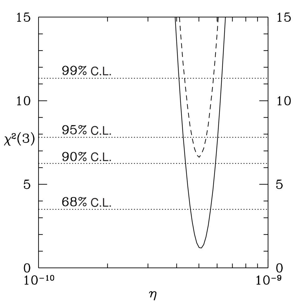
FIG. 2.: $\chi^{2}$ as a function of $\eta$, for SBBN with three degrees of freedom $(\eta,\tau_{X},m_{X}Y_{X})$. We show our results for both of the ⁴He abundances deduced from observation: low ⁴He (dashed), high ⁴He (solid).

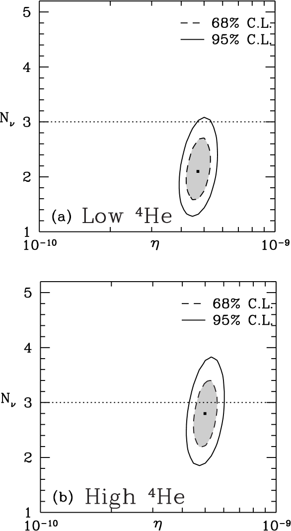
FIG. 3.: Figure 3: C.L. for BBN as a function of $\eta$ and $N_{\nu}$, with (a) low value of $Y$, and (b) high value of $Y$. The filled square denotes the best-fit point.

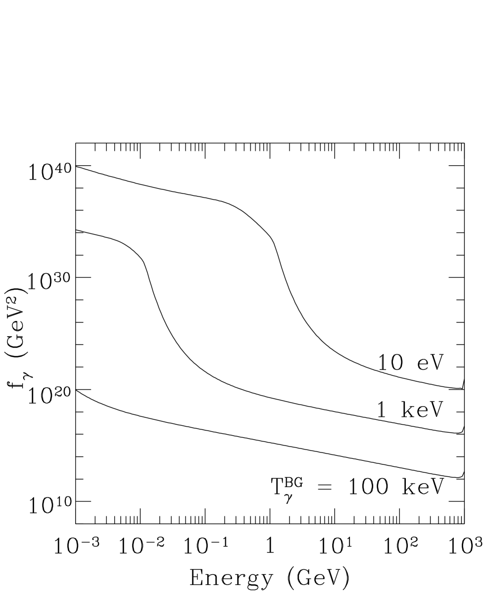
FIG. 4.: Photon spectrum $f_{\gamma}=dn_{\gamma}/dE_{\gamma}$ for several background temperatures $T_{\gamma}^{\rm BG}$.

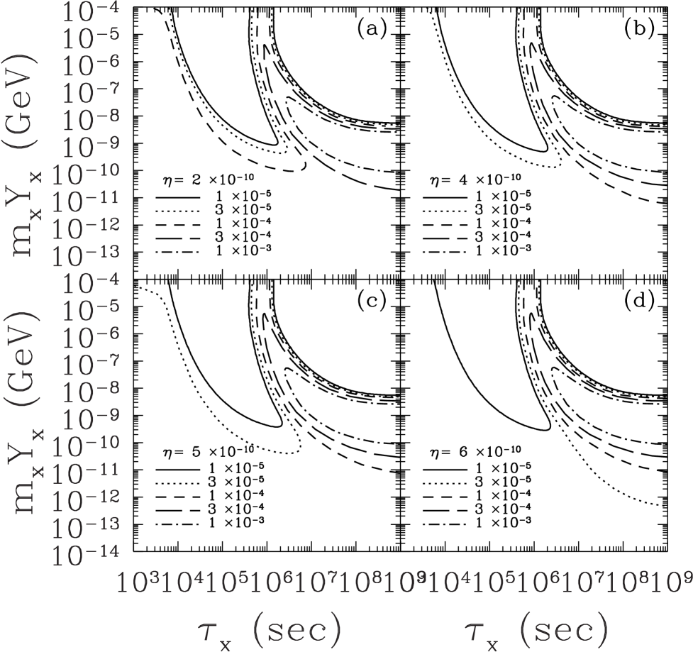
FIG. 5.: The abundance of D/H in the $m_{X}Y_{X}$ vs. $\tau_{X}$ plane with (a) $\eta=2\times 10^{-10}$, (b) $\eta=4\times 10^{-10}$, (c) $\eta=5\times 10^{-10}$, and (d) $\eta=6\times 10^{-10}$.

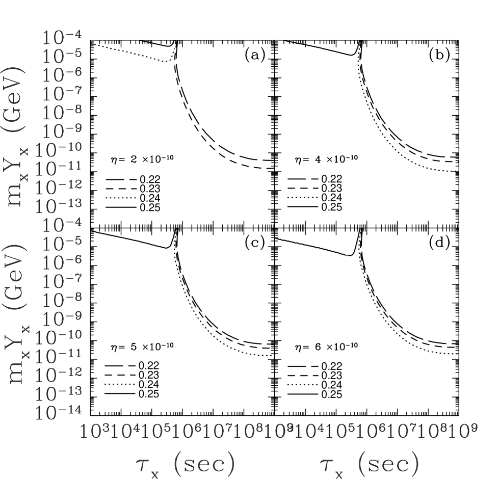
FIG. 6.: The mass fraction of ⁴He, for the same theory parameters as in Fig. 5.

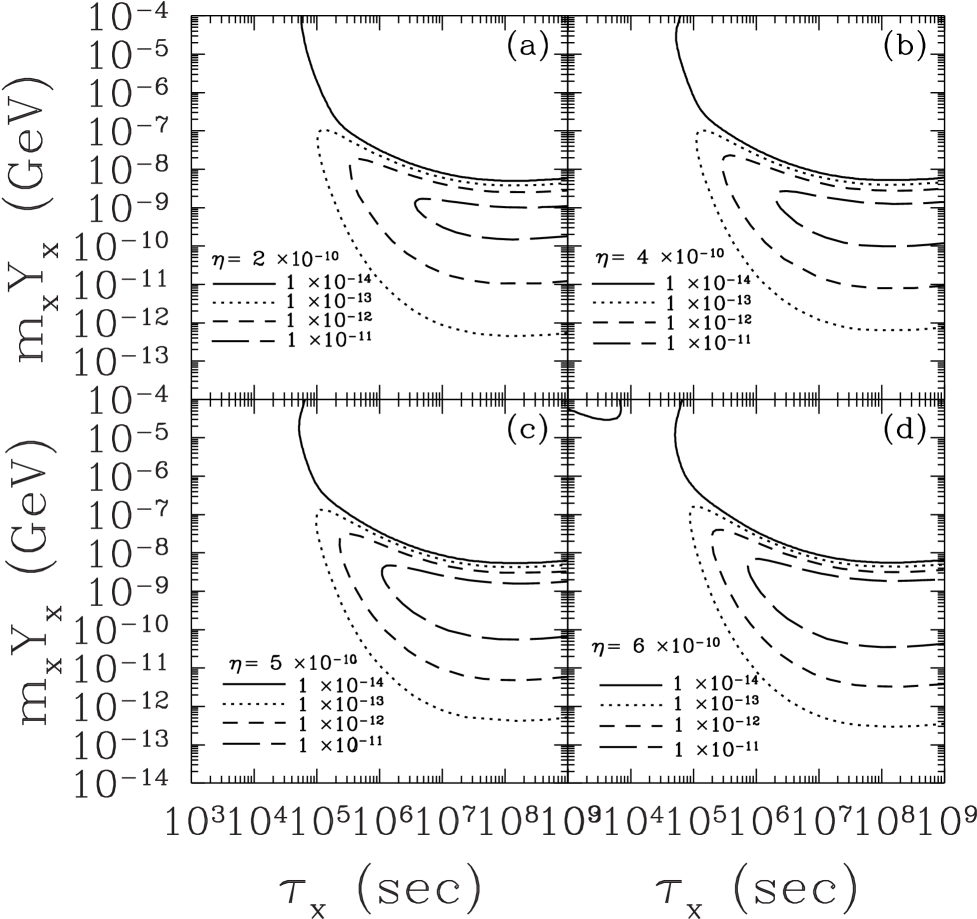
FIG. 7.: The abundance of ⁶Li/H, for the same theory parameters as in Fig. 5.

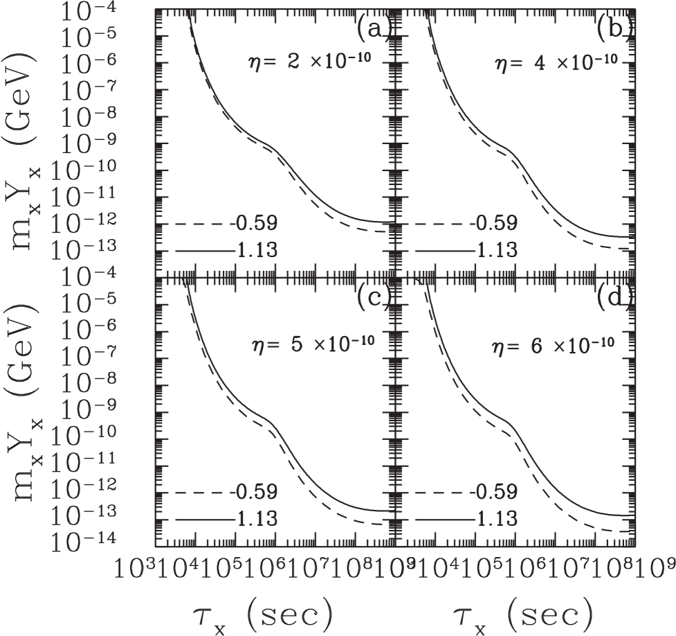
FIG. 8.: The abundance of ³He/D, for the same theory parameters as in Fig. 5.

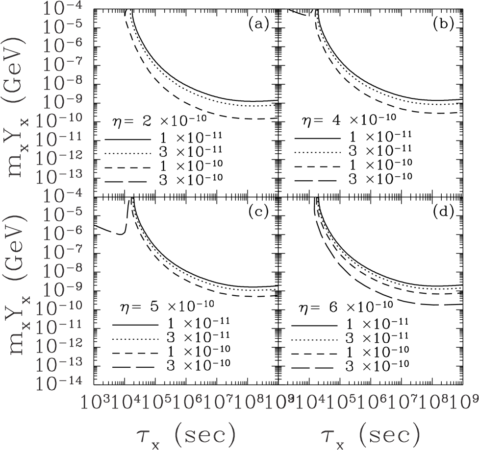
FIG. 9.: The abundance of ⁷Li/H, for the same theory parameters as in Fig. 5.

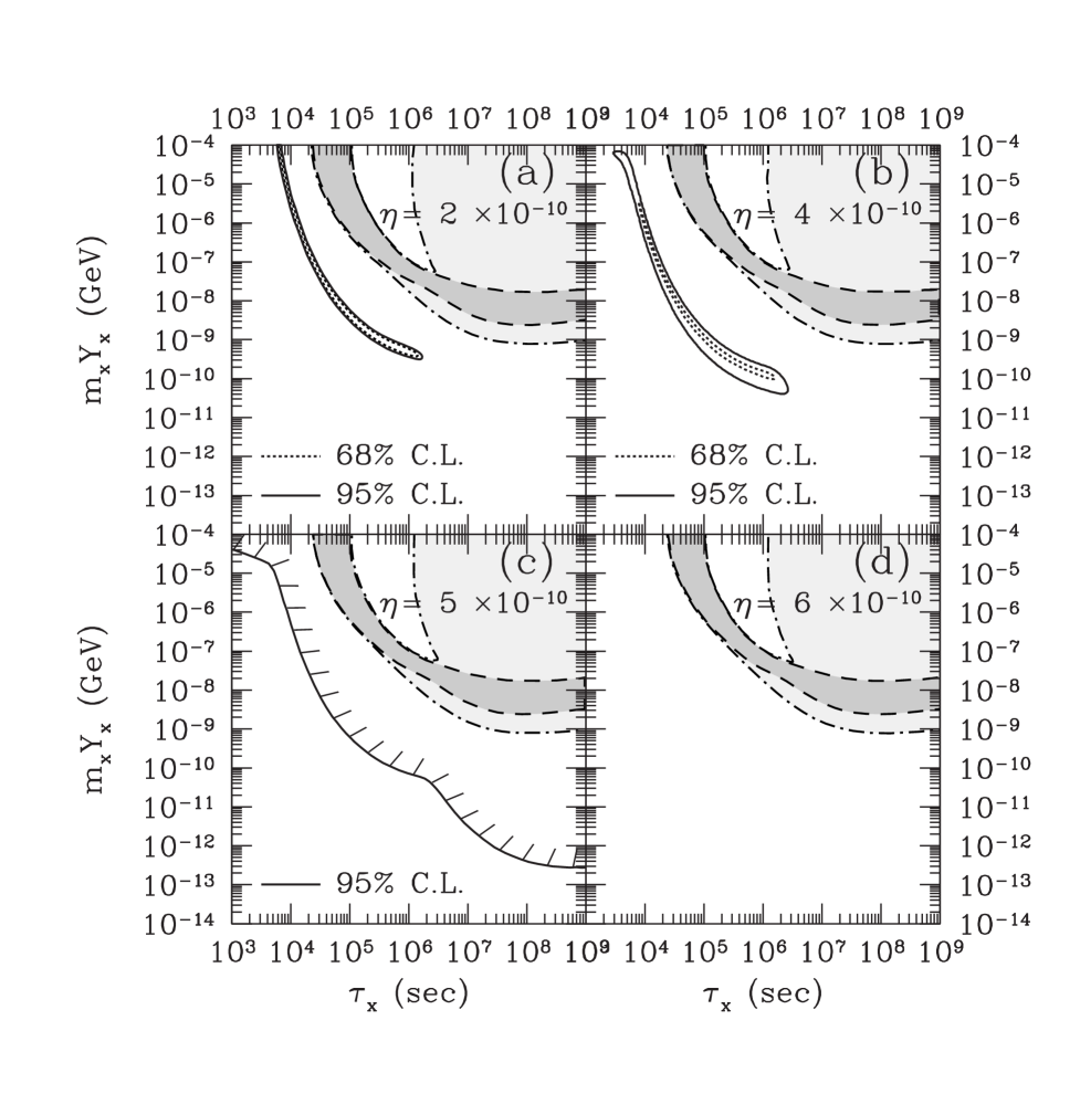
FIG. 10.: C.L. in the $m_{X}Y_{X}$ vs. $\tau_{X}$ plane, for low value of $Y$. We take (a) $\eta=2\times 10^{-10}$, (b) $\eta=4\times 10^{-10}$, (c) $\eta=5\times 10^{-10}$, and (d) $\eta=6\times 10^{-10}$. The shaded regions are $y_{6}/y_{7}\geq 0.5$, and the darker shaded regions are $y_{6}/y_{7}\geq 1.3$.

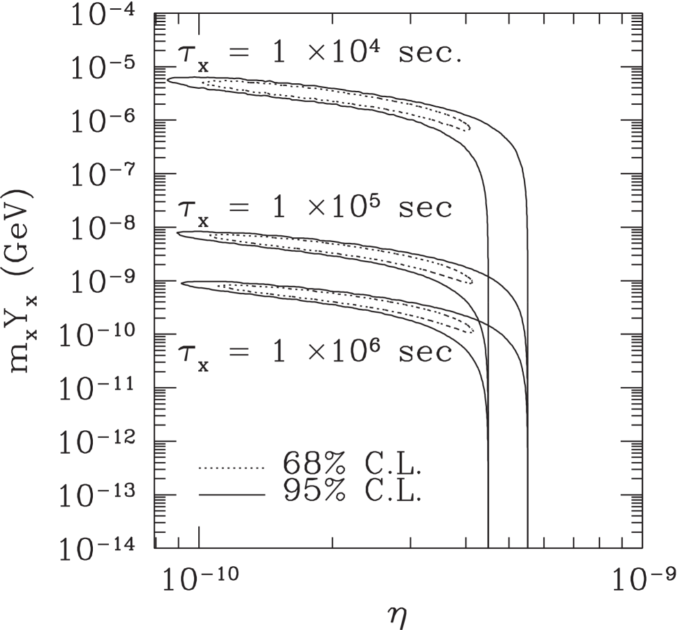
FIG. 11.: C.L. in the $\eta$ vs. $m_{X}Y_{X}$ plane for various values of $\tau_{X}$, for low value of $Y$.

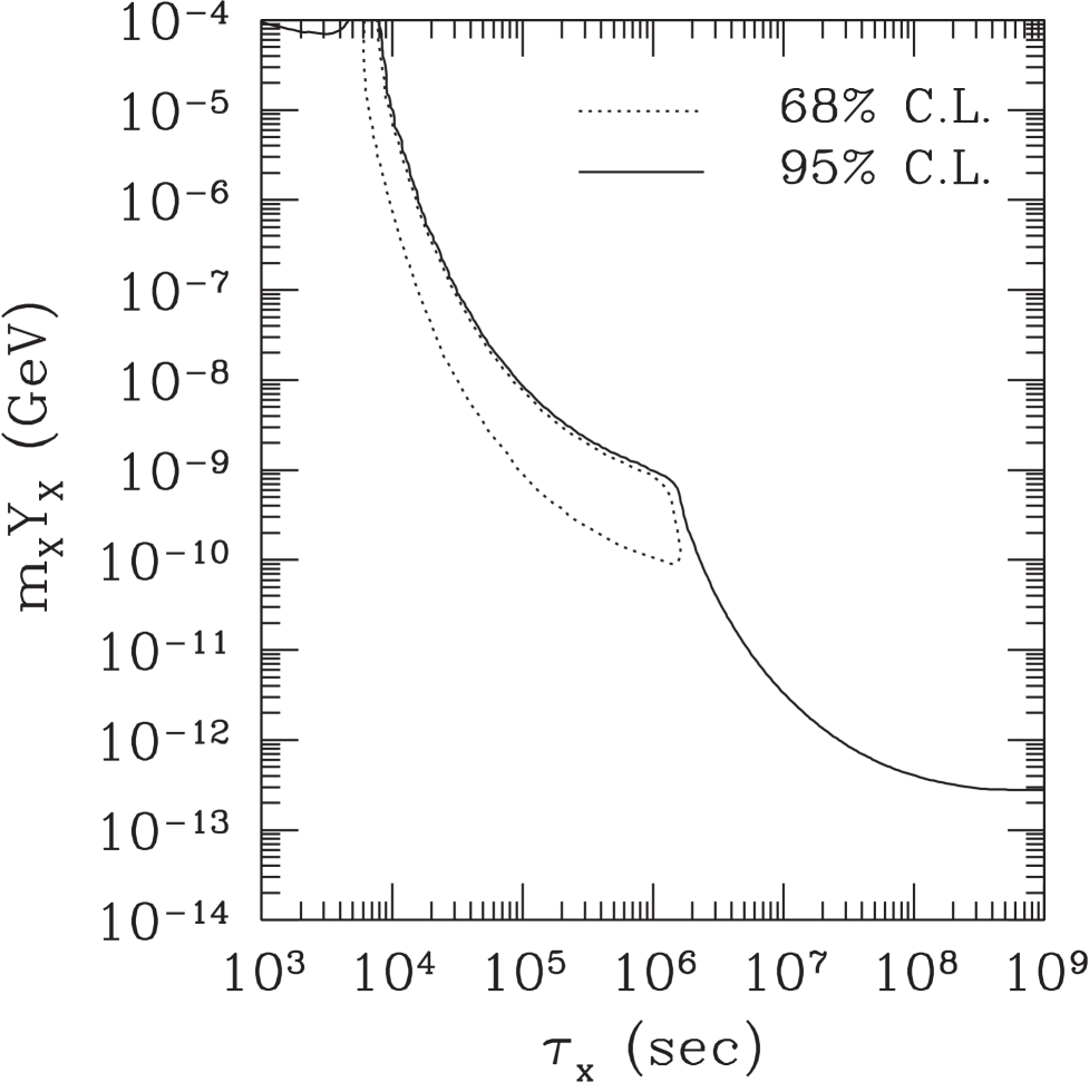
FIG. 12.: Contours of C.L. projected on $\eta$ axis for low value of $Y$.

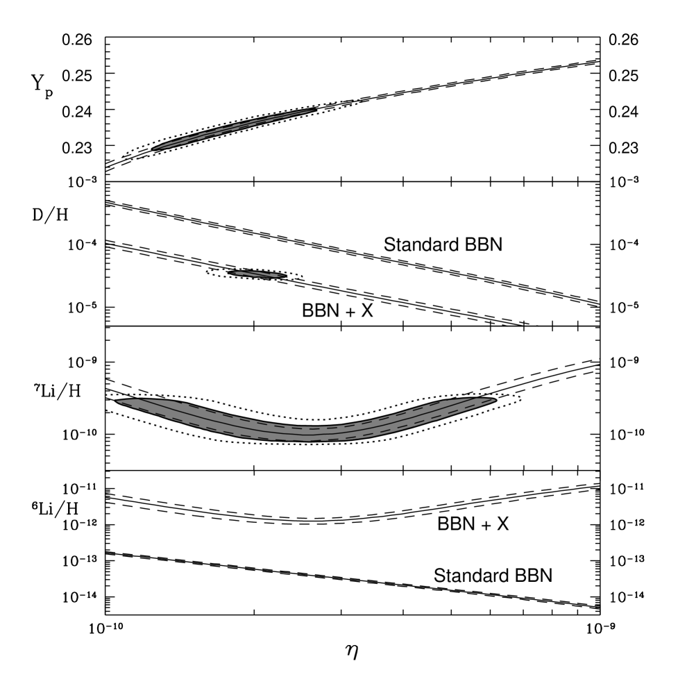
FIG. 13.: Predicted light-element abundances ⁴He, D, ⁷Li and ⁶Li at $\tau_{X}=10^{6}$ sec and $m_{X}Y_{X}=5\times 10^{-10}$ GeV. The contours which are favored by observation are plotted, adopting the low ⁴He and low D values. The dotted line denotes the 95% C.L. and the shaded region denotes the 68% C.L.. The predicted ⁶Li abundance is two orders of magnitude larger than the case of SBBN.

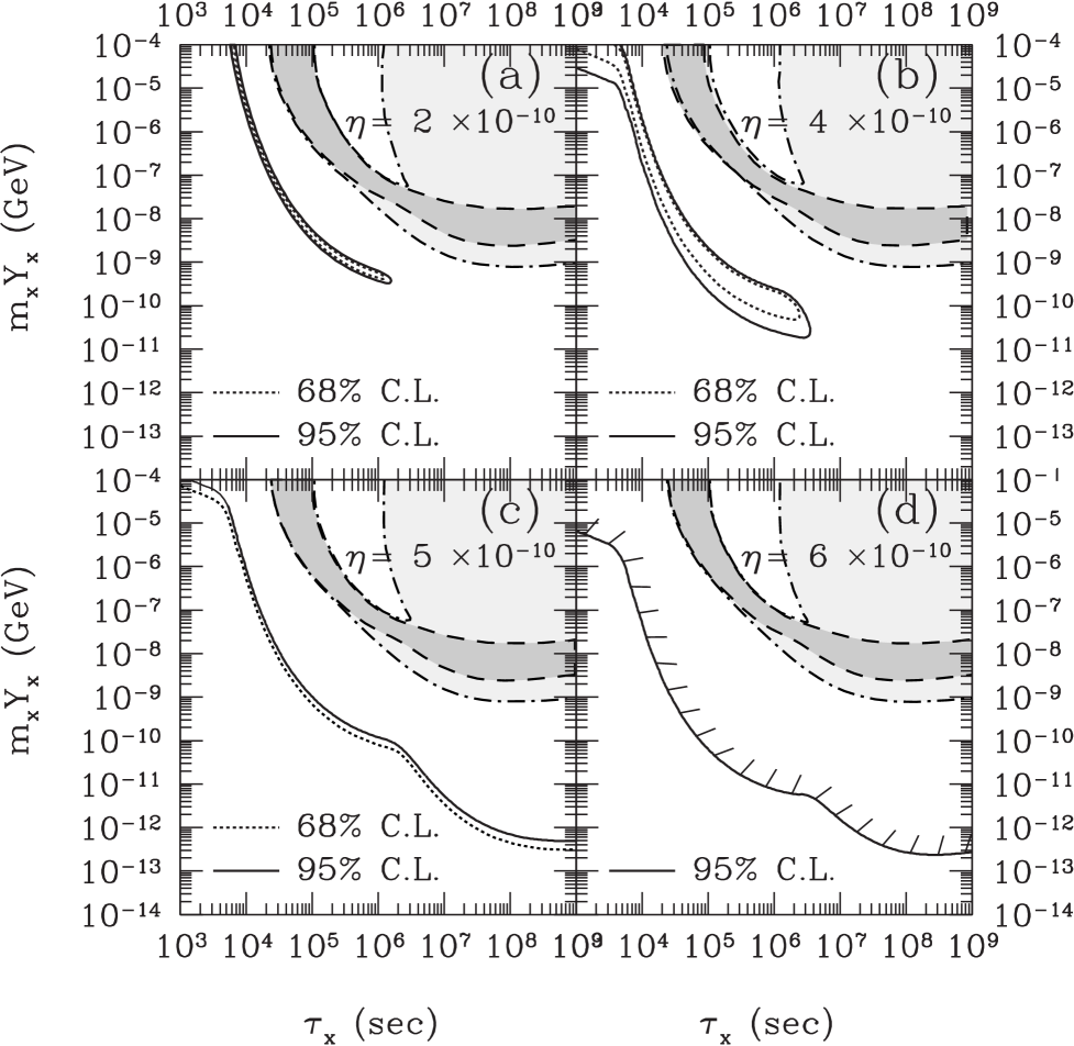
FIG. 14.: Same as Fig. 10, except for high value of $Y$.

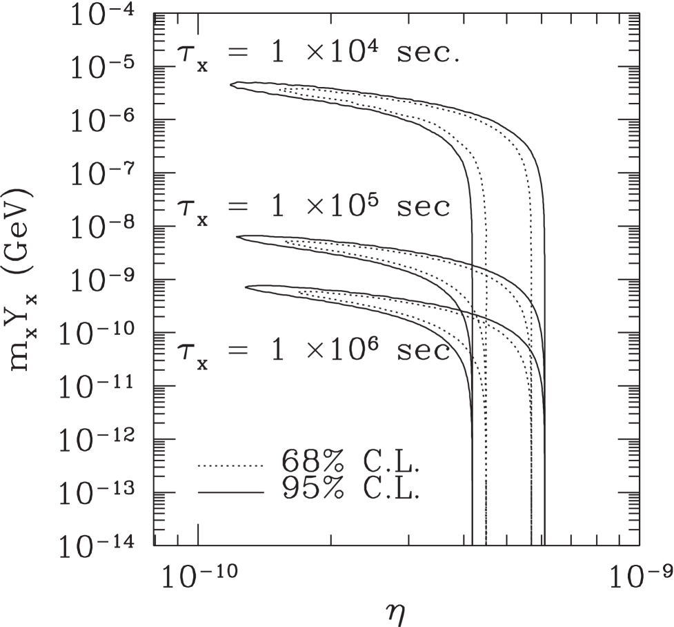
FIG. 15.: Same as Fig. 11, except for high value of $Y$.

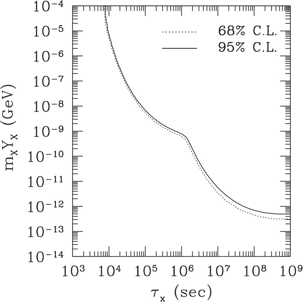
FIG. 16.: Same as Fig. 12, except for high value of $Y$. The region above the solid line is excluded at the 95% C.L., while the region above the dotted line is excluded at the 95% C.L.

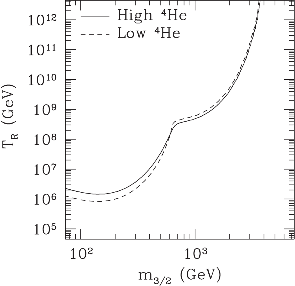
FIG. 17.: Contours of 95% C.L., yielding an upper bound on the reheating temperature, as a function of the gravitino mass. These are the results of the two-photon emission by the decay of a gravitino. If we consider the one-photon emission such as $\psi_{\mu}\to\tilde{\gamma}+\gamma$, the upper bounds become milder by a factor of two.

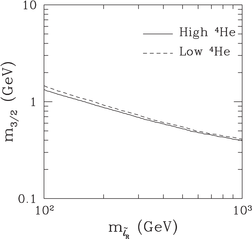
FIG. 18.: Contours of 95% C.L., yielding an upper bound on the gravitino mass, as a function of the right-handed slepton mass.

REFERENCES

- [1] T.P. Walker, G. Steigman, D.N. Schramm, K.A. Olive, and H.-S. Kang, Astrophys. J. 376 (1991) 51; Subir Sarkar, Rept. Prog. Phys. 59 (1996) 1493, hep-ph/9602260.
- [2] D. Lindley, Mon. Not. Roy. Astron. Soc. 188 (1979) 15P; D. Lindley, Astrophys. J. 294 (1985) 1.
- [3] H. Pagels and J.R. Primack, Phys. Rev. Lett. 48 (1982) 223; S. Weinberg, Phys. Rev. Lett. 48 (1982) 1303; L.M. Krauss, Nucl. Phys. B227 (1983) 556; J. Ellis, E. Kim, and D.V. Nanopoulos, Phys. Lett. B145 (1984) 181; R. Juszkiewicz, J. Silk, and A. Stebbins, Phys. Lett. B158 (1985) 463; J. Ellis, E. Kim, and S. Sarkar, Nucl. Phys. B259 (1985) 175; M. Kawasaki and K. Sato, Phys. Lett. B189 (1987) 23; J. Ellis, G.B. Gelmini, J.L. Lopez, D.V. Nanopoulos, and S. Sarkar, Nucl. Phys. B373 (1992) 399; T. Moroi, H. Murayama, and M. Yamaguchi, Phys. Lett. B303 (1993) 289.
- [4] M. Kawasaki and T. Moroi, Prog. Theor. Phys. 93 (1995) 879, hep-ph/9403364.
- [5] M. Kawasaki and T. Moroi, Astrophys. J. 452 (1995) 506, astro-ph/9412055.
- [6] S. Dimopoulos, R. Esmailzadeh, L.J. Hall, and G.D. Starkman, Astrophys. J. 330 (1988) 545; Nucl. Phys. B311 (1989) 699.
- [7] S. Dimopoulos, G. Dvali, R. Rattazzi, and G.F. Giudice, Nucl. Phys. B510 (1998) 12, hep-ph/9705307.
- [8] N. Hata, R.J. Scherrer, G. Steigman, D. Thomas, T.P. Walker, S. Bludman, and P. Langacker, Phys. Rev. Lett. 75 (1995) 3977, hep-ph/9505319.
- [9] K. Kohri, M. Kawasaki, and K. Sato, Astrophys. J. 490 (1997) 72, astro-ph/9612237.
- [10] M. Kawasaki, K. Kohri, and K. Sato, Phys. Lett. B430 (1998) 132, astro-ph/9705148.
- [11] E. Holtmann, M. Kawasaki, and T. Moroi, Phys. Rev. Lett. 77 (1996) 3712, hep-ph/9603241.
- [12] B.E.J. Pagel et al., Mon. Not. R. Astron. Soc. 255 (1992) 325.
- [13] K.A. Olive, G. Steigman, and E.D. Skillman, Astrophys. J. 483 (1997) 788.
- [14] Y.I. Izotov, T.X. Thuan, and V.A. Lipovetsky, Astrophys. J., 435 (1994) 647.
- [15] T.X. Thuan and Y.I. Izotov, in Primordial Nuclei and their Galactic Evolution, edited by N. Prantzos, M. Tosi, and R. von Steiger (Kluwer Academic Publications, Dordrecht, 1998) in press.
- [16] Y.I. Izotov, T.X. Thuan, and V.A. Lipovetsky, Astrophys. J. Suppl. Series, 108 (1997) 1.
- [17] P.J. Kernan and S. Sarkar, Phys. Rev. D54 (1996) R3681, astro-ph/960304.
- [18] A.D. Dolgov and B.E.J. Pagel, astro-ph/9711202; K. Jedamzik and G.M. Fuller, Astrophys. J., 452 (1995) 33.
- [19] S. Burles and D. Tytler, submitted to Astrophys. J., astro-ph/9712109.
- [20] A. Songaila, L.L. Cowie, C.J. Hogan, and M. Rugers, Nature 368 (1994) 599.
- [21] R.F. Carswell, M. Rauch, R.J. Weymann, A.J. Cooke, and J.K. Webb, Mon. Not. Roy. Astron. Soc. 268 (1994) L1.
- [22] M. Rugers and C.J. Hogan, Astrophys. J., Lett. 459 (1996) L1.
- [23] J. K. Webb et al., Nature 388 (1997) 250.
- [24] E. Holtmann, in preparation.
- [25] J. Geiss, in Origin and Evolution of the Elements, edited by N. Prantzos, E. Vangioni-Flam, and M. Cassé (Cambridge University Press, Cambridge, 1993) 89.
- [26] G. Sigl, K. Jedamzik, D.N. Schramm, and V.S. Berezinsky, Phys. Rev. D52 (1995) 6682, astro-ph/9503094.
- [27] F. Spite and M. Spite, Astronomy and Astrophysics 115 (1982), 357.
- [28] P. Bonifacio and P. Molaro, Mon. Not. Roy. Astron. Soc. 285 (1997) 847.
- [29] C.J. Hogan, astro-ph/9609138.
- [30] B.D. Fields, K. Kainulainen, K.A. Olive, and D. Thomas, New Astron. 1 (1996) 77, astro-ph/9603009.
- [31] L.M. Hobbs and J.A. Thorburn, Astrophys. J. 491 (1997) 772.
- [32] V.V. Smith, D.L. Lambert, and P.E. Nissen, Astrophys. J. 408 (1993) 262.
- [33] L. Kawano, preprint FERMILAB-Pub-92/04-A.
- [34] Particle Data Group, Phys. Rev. D54 (1996) 1.
- [35] G.R. Caughlan and W.A. Fowler, Atomic Data and Nuclear Data Tables 40 (1988) 283; M.S. Smith, L.H. Kawano, and R.A. Malaney, Astrophys. J. Suppl. Series 85 (1993) 219.
- [36] G. Fiorentini, E. Lisi, S. Sarkar, and F. L. Villante, astro-ph/9803177.
- [37] J. Yang, M.S. Turner, G. Steigman, D.N. Schramm, and K.A. Olive, Astrophys. J. 281 (1984) 493.
- [38] C.J. Copi, D.N. Schramm, and M.S. Turner, Phys. Rev. Lett. 75 (1995) 3981, astro-ph/9508029.
- [39] A.A. Zdziarski, Astrophys. J. 335 (1988) 786; R. Svensson and A.A. Zdziarski, Astrophys. J. 349 (1990) 415.
- [40] R.D. Evans, The Atomic Nucleus (McGraw-Hill, New York, 1955).
- [41] R. Pfeiffer, Z. Phys. 208 (1968) 129.
- [42] D.D. Faul, B.L. Berman, P. Mayer, and D.L. Olson, Phys. Rev. Lett. 44 (1980) 129.
- [43] A.N. Gorbunov and A.T. Varfolomeev, Phys. Lett. 11 (1964) 137.
- [44] J.D. Irish, R.G. Johnson, B.L. Berman, B.J. Thomas, K.G. McNeill, and J.W. Jury, Can. J. Phys. 53 (1975) 802.
- [45] C.K. Malcom, D.V. Webb, Y.M. Shin, and D.M. Skopik, Phys. Lett. B47 (1973) 433.
- [46] Yu.M. Arkatov, P.I. Vatset, V.I. Voloshchuk, V.A. Zolenko, I.M. Prokhorets, and V.I. Chimil’, Sov. J. Nucl. Phys. 19 (1974) 598.
- [47] B.L. Berman, Atomic Data and Nuclear Data Tables 15 (1975) 319.
- [48] D.J. Fixsen et al., Astrophys. J 473 (1996) 576.
- [49] W. Hu and J. Silk, Phys. Rev. Lett. 70 (1993) 2661.
- [50] A.P. Lightman, Astrophys. J. 244 (1981) 392.
- [51] J. Gratsias, R.J. Scherrer, and D.N. Spergel, Phys. Lett. B262 (1991) 298; M. Kawasaki and T. Moroi, Phys. Lett. B346 (1995) 27, hep-ph/9408321.
- [52] K.A. Olive and M. Srednicki, Phys. Lett. B230 (1989) 78.
- [53] E.W. Kolb and M.S. Turner, The Early Universe (Addison-Wesley, 1990).
- [54] B. de Carlos, J.A. Casas, F. Quevedo, and E. Roulet, Phys. Lett. B318 (1993) 447, hep-ph/9308325.
- [55] D.H. Lyth and E.D. Stewart, Phys. Rev. Lett. 75 (1995) 201, hep-ph/9502417; Phys. Rev. D53 (1996) 1784, hep-ph/9510204.