Universal $\tau_{1/2}(y)$ Isgur-Wise function
at the next-to-leading order in QCD sum rules

Abstract

We use QCD sum rules, in the framework of the Heavy Quark Effective Theory, to calculate the universal form factor $\tau_{1/2}(y)$ parameterizing the semileptonic transitions $B\to D_{0}\ell\bar{\nu}$, $B\to D_{1}^{*}\ell\bar{\nu}$, where $D_{0}$ and $D^{*}_{1}$ are the members of the excited charmed doublet with $J^{P}=(0^{+}_{1/2},1^{+}_{1/2})$. We include two-loop corrections in the perturbative contribution to the sum rule, and present a complete next-to-leading order result. As a preliminary part of our analysis we also compute, up to order $\alpha_{s}$, the leptonic constant $F^{+}$ of the doublet $D_{0}$, $D_{1}^{*}$. Finally, we discuss the phenomenological implications of this calculation.

I Introduction

The application of the heavy quark flavor and spin symmetry, valid in QCD in the infinite heavy quark mass limit [1, 2], together with the heavy quark effective field theory (HQET) [3, 4, 5], has led to a dramatic progress towards a model-independent description of the spectroscopy and the decays of hadrons containing a single heavy quark $Q$ ($Q=c,b$). An outstanding result of the theory concerns the description of the exclusive $B\to D\ell\bar{\nu}$ and $B\to D^{*}\ell\bar{\nu}$ semileptonic decays, in the limit $m_{Q}\to\infty$, in terms of just one nonperturbative, universal form factor (the Isgur-Wise function $\xi$), normalized to unity at maximum momentum transfer to the lepton pair. Other distinctive examples are the relations between the beauty meson leptonic constants and the beauty meson semileptonic transition amplitudes to light mesons at zero recoil, with the analogous charmed meson ones, obtained employing general dimensional scaling rules.

Corrections of order $\Lambda_{QCD}/m_{Q}$ (and higher powers) to the leading term can be systematically analyzed in HQET in terms of a reduced number of hadronic, universal parameters, with a remarkable simplification of the analysis. However, in the applications of HQET the effects of non-perturbative strong interactions can be estimated only in the framework of some non-perturbative theoretical approach. In this regard, particularly fruitful has been the application of sum rules [6] formulated in the framework of HQET [7]. This method is genuinely field theoretical and based on first principles, and relates the hadronic observables to QCD fundamental parameters via the Operator Product Expansion (OPE) of suitable Green’s functions. Such an expansion involves perturbative contributions as well as non-perturbative quark and gluon vacuum condensates. In particular, $\alpha_{s}$ corrections to the coefficients of the OPE can be computed order by order in perturbation theory, and therefore they can be systematically taken into account.

A critical aspect of the sum rule calculations in HQET is represented by the size of non-leading terms, such as the $1/m_{Q}$ corrections and the $\alpha_{s}$ corrections in the perturbative expansion of the OPE. For example, the predictions for the leptonic constants of $\bar{q}Q$ pseudoscalar mesons are affected by considerably large next-to-leading corrections in $\alpha_{s}$ [8, 9, 10]; also $\Lambda_{QCD}/m_{Q}$ corrections are non-negligible in the case of the $D$ meson, an effect confirmed by lattice QCD analyses [11].

Conversely, in the HQET QCD sum rule calculation of the Isgur-Wise function, the next-to-leading order $\alpha_{s}$ corrections turn out to be small and well under control [12, 13], and the same is true for $\Lambda_{QCD}/m_{Q}$ corrections [14], specially near the zero recoil point where the normalization of the universal form factor is protected by the heavy quark symmetry. This has allowed a drastic reduction of the theoretical uncertainty in the determination of the CKM matrix element $V_{cb}$ [15].

It is worth analyzing other cases analogous to the determination of the Isgur-Wise form factor $\xi$, and we present here a HQET sum rule calculation of the universal form factor governing the semileptonic $B$ meson decays into the $0^{+},1^{+}$ charmed excited states, up to next-to-leading order in $\alpha_{s}$ and to leading order in the heavy quark expansion $m_{Q}\to\infty$. These higher-lying charmed states correspond to the $L=1$ orbital excitations in the non-relativistic constituent quark model. Besides their theoretical relevance to HQET [16], in particular to the aspects of the QCD sum rule calculation mentioned above, such $B\to D^{**}$ semileptonic transitions ($D^{**}$ is the generic $L=1$ charmed state) have numerous additional points of physical interest.

Indeed, in principle these decay modes may account for a sizeable fraction of semileptonic $B$-decays, and consequently they represent a well-defined set of corrections to the theoretical prediction that, in the limit $m_{Q}\to\infty$ and under the condition $(m_{b}-m_{c})/(m_{b}+m_{c})\to 0$ (the so-called small-velocity limit), the total semileptonic $B\to X_{c}$ decay rate should be saturated by the $B\to D$ and $B\to D^{*}$ modes [2]. Moreover, the shape of the inclusive differential decay distribution in the lepton energy could reflect contributions from the $B\to D^{**}$ modes.

Another important result, relevant both to phenomenology and to the critical tests of HQET, is the relation of the $B\to D^{**}$ form factors at zero recoil to the slope of the $B\to D^{(*)}$ Isgur-Wise function, through the Bjorken sum rule [17]. Of similar interest for HQET is the test of the upper bound on such universal form factors at zero recoil, involving the heavy meson “binding energy” and the $D^{**}-D$ mass splittings, that is the analog of the “optical” sum rule for dipole scattering of light in atomic physics [18, 19].

Moreover, the $\Lambda_{QCD}/m_{Q}$ corrections can have a role for $B$-decay modes into excited charmed states, that mostly occur near the zero recoil point where the corresponding transition matrix elements vanish. The shape of the lepton energy spectrum near such kinematical point including the $1/m_{Q}$ corrections, that in HQET can be predicted in terms of the Isgur-Wise function and mesons mass splittings, represents an important test of the theory [20].

Continuing with the aspects justifying the interest for $B\to D^{**}$, let us notice that the investigation of the semileptonic $B$ transitions to excited charm states is an important preliminary study for the theoretical analysis of the production of such states in nonleptonic $B$ decays [21], as well as for the identification of additional decay modes (such as $D^{(*)}D^{(*)}\pi$) suitable for the investigation of CP violating effects at $B$ factories [22].

Finally, as a byproduct of the QCD sum rule calculation, theoretical predictions about the yet unobserved $D^{**}$ meson masses can be obtained, that are obviously interesting per se.

In the following we present a complete next-to-leading order evaluation of the $B$-meson semileptonic transition to the scalar charmed state by QCD sum rules, at the leading order of $m_{b,c}\to\infty$. In Sect. II we report the main aspects of the spectroscopy and decays of $L=1$ $\bar{q}Q$ mesons, together with the definition of the universal form factor $\tau_{1/2}(y)$. The various steps of the QCD sum rule determination of such form factor, within HQET, are collected in Sect. III and V-VII, together with the analysis, in Sect. IV, of the leptonic constant $F^{+}$ of the doublet $D_{0},D^{*}_{1}$. In Sect. VIII the phenomenological implications of our calculation are presented, together with the conclusions.

II Positive Parity heavy-light mesons

In the infinite heavy quark mass limit the spectrosopy of hadrons containing one heavy quark Q is greatly simplified, due to the decoupling of the heavy quark spin $\vec{s}_{Q}$ from the angular momentum of the light degrees of freedom (quarks and gluons) $\vec{s}_{\ell}=\vec{J}-\vec{s}_{Q}$. This allows a classification of such hadronic states by $\vec{J}$ and by $\vec{s}_{\ell}$, so that hadrons corresponding to the same $s_{\ell}$ belong to degenerate doublets. In the case of $\bar{q}Q$ mesons, the low-lying states with $s_{\ell}^{P}={1\over 2}^{-}$ correspond to the pseudoscalar $0^{-}$ and vector $1^{-}$ mesons ($B,B^{*}$; $D,D^{*}$), the $s$-wave states of the constituent quark model. The four states corresponding to orbital angular momentum $L=1$ can be classified in two doublets: $J^{P}=(0^{+}_{1/2},1^{+}_{1/2})$ and $J^{P}=(1^{+}_{3/2},2^{+}_{3/2})$, which differ by the values $s_{\ell}^{P}={1\over 2}^{+}$ and $s_{\ell}^{P}={3\over 2}^{+}$, respectively. The states $0^{+}_{1/2}$ and $2^{+}_{3/2}$ correspond to the scalar and spin-two mesons of the quark model; the relation between HQET and quark model $L=1$, $1^{+}$ states can easily be derived [23].

The charmed $2^{+}_{3/2}$ state has been experimentally observed and denoted as the $D_{2}^{*}(2460)$ meson, with $m_{D_{2}^{*}}=2458.9\pm 2.0$ MeV, $\Gamma_{D_{2}^{*}}=23\pm 5$ MeV and $m_{D_{2}^{*}}=2459\pm 4$ MeV, $\Gamma_{D_{2}^{*}}=25^{+8}_{-7}$ MeV for the neutral and charged states, respectively [24]. The HQET state $1^{+}_{3/2}$ can be identified with $D_{1}(2420)$, with $m_{D_{1}}=2422.2\pm 1.8$ MeV and $\Gamma_{D_{1}}=18.9^{+4.6}_{-3.5}$ MeV [24], even though a $1^{+}_{1/2}$ component can be contained in such physical state due to the mixing allowed for the finite value of the charm quark mass.

Both the states $2^{+}_{3/2}$ and $1^{+}_{3/2}$ decay to hadrons by $d-$wave transitions, which explains their narrow width; the strong coupling constant governing their two-body decays can be determined using experimental information [26]. On the other hand, the $s_{\ell}^{P}={1\over 2}^{+}$ doublet ($D_{0},D^{*}_{1}$) has not been observed yet. The strong decays of such states occur through $s$-wave transitions, with expected larger widths than in the case of the doublet ${3\over 2}^{+}$. Indeed, analyses of the coupling constant governing the two-body hadronic transitions by QCD sum rules predict $\Gamma(D_{0}^{0}\to D^{+}\pi^{-})\simeq 180$ MeV and $\Gamma(D_{1}^{*0}\to D^{*+}\pi^{-})\simeq 165$ MeV [27] . Estimates of the mixing angle $\alpha$ between $D^{*}_{1}$ and $D_{1}$ give $\alpha\simeq 16^{0}$ [27, 28].

The matrix elements of the semileptonic $B\to D_{0}\ell\bar{\nu}$ and $B\to D_{1}^{*}\ell\bar{\nu}$ transitions can be parameterized in terms of six form factors:

$${<D_{0}(v^{\prime})|{\bar{c}}\gamma_{\mu}\gamma_{5}b|B(v)>\over{\sqrt{m_{B}m_{D_{0}}}}} = g_{+}(v+v^{\prime})_{\mu}+g_{-}(v-v^{\prime})_{\mu}$$ (1)

$${<D^{*}_{1}(v^{\prime},\epsilon)|{\bar{c}}\gamma_{\mu}(1-\gamma_{5})b|B(v)>\over{\sqrt{m_{B}m_{D^{*}_{1}}}}} = g_{V_{1}}\epsilon^{*}_{\mu}+\epsilon^{*}\cdot v\;[g_{V_{2}}v_{\mu}+g_{V_{3}}v^{\prime}_{\mu}]-i\;g_{A}\epsilon_{\mu\alpha\beta\gamma}\epsilon^{*\alpha}v^{\beta}v^{\prime\gamma}\;\;\;,$$ (2)

where $v$ and $v^{\prime}$ are four-velocities and $\epsilon$ is the $D_{1}^{*}$ polarization vector. The form factors $g_{i}$ depend on the variable $y=v\cdot v^{\prime}$, which is directly related to the momentum transfer to the lepton pair. In terms of such form factors the semileptonic differential decay rates can be expressed as

$${d\Gamma\over dy}(B\to D_{0}\ell\nu) = {G_{F}^{2}|V_{cb}|^{2}m_{B}^{5}\over 48\pi^{3}}(y^{2}-1)^{3/2}\Big{(}{m_{D_{0}}\over m_{B}}\Big{)}^{3}\Big{[}\Big{(}1+{m_{D_{0}}\over m_{B}}\Big{)}g_{+}-\Big{(}1-{m_{D_{0}}\over m_{B}}\Big{)}g_{-}\Big{]}^{2}$$ (3)

$${d\Gamma\over dy}(B\to D_{1}^{*}\ell\nu) = {G_{F}^{2}|V_{cb}|^{2}m_{B}^{5}\over 48\pi^{3}}\sqrt{y^{2}-1}\Big{(}{m_{D_{1}^{*}}\over m_{B}}\Big{)}^{3}\Big{\{}\Big{[}\Big{(}y-{m_{D_{1}^{*}}\over m_{B}}\Big{)}g_{V_{1}}+(y^{2}-1)\Big{(}g_{V_{3}}+{m_{D_{1}^{*}}\over m_{B}}g_{V_{2}}\Big{)}\Big{]}^{2}$$ (4)

$$+ 2\Big{[}1-2{m_{D_{1}^{*}}\over m_{B}}y+\Big{(}{m_{D_{1}^{*}}\over m_{B}}\Big{)}^{2}\Big{]}[g_{V_{1}}^{2}+(y^{2}-1)g_{V_{A}}^{2}]\Big{\}}\;\;\;.$$ (5)

The heavy quark spin symmetry allows to relate the form factors $g_{i}(y)$ in (2) to a single function $\tau_{1/2}(y)$ [16] through short-distance coefficients, perturbatively calculable, which depend on the heavy quark masses $m_{b},m_{c}$, on $y$ and on a mass-scale $\mu$, and connect the QCD vector and axial vector currents to the HQET currents. At the next-to-leading logarithmic approximation in $\alpha_{s}$ and in the infinite heavy quark mass limit, the relations between $g_{i}$ and $\tau_{1/2}$ are given by

$$g_{+}(y)+g_{-}(y) = -2\;\Big{(}C_{1}^{5}(\mu)+(y-1)C_{2}^{5}(\mu)\Big{)}\;\tau_{1/2}(y,\mu)$$ (6)

$$g_{+}(y)-g_{-}(y) = 2\;\Big{(}C_{1}^{5}(\mu)-(y-1)C_{3}^{5}(\mu)\Big{)}\;\tau_{1/2}(y,\mu)$$ (7)

$$g_{V_{1}}(y) = 2(y-1)\;C_{1}(\mu)\;\tau_{1/2}(y,\mu)$$ (8)

$$g_{V_{2}}(y) = -2\;C_{2}(\mu)\;\tau_{1/2}(y,\mu)$$ (9)

$$g_{V_{3}}(y) = -2\;\Big{(}C_{1}(\mu)+C_{3}(\mu)\Big{)}\;\tau_{1/2}(y,\mu)$$ (10)

$$g_{A}(y) = -2\;C_{1}^{5}(\mu)\;\tau_{1/2}(y,\mu)\;.$$ (11)

The $\mu$-dependence is the same for all the functions $C_{i}^{(5)}$, where $C_{i}$ refer to the vector current and $C_{i}^{5}$ to the axial one; therefore, one can extract such a dependence by writing [7]

$$C_{i}^{(5)}(\mu)={\hat{C}}_{i}^{(5)}(m_{b},m_{c},y)\;K_{hh}(y,\mu)$$ (12)

where $K_{hh}=[\alpha_{s}(\mu)]^{-a_{hh}(y)}\Big{\{}1-{\alpha_{s}(\mu)\over\pi}Z_{hh}(y)\Big{\}}$, with $a_{hh}={2\over 9}\gamma(y)$,

$$\gamma(y)={4\over 3}[yr(y)-1]$$ (13)

and $r(y)={\ln(y+\sqrt{y^{2}-1})\over\sqrt{y^{2}-1}}$, is related to the velocity-dependent anomalous dimension of the heavy-heavy $b\to c$ current in HQET [4]. The coefficient $Z_{hh}$, derived in [7, 9, 29] has the expansion, for $n_{f}=3$:

$$Z_{\rm hh}(y)=\bigg{(}{752\over 729}-{8\pi^{2}\over 81}\bigg{)}(y-1)-\bigg{(}{368\over 1215}-{4\pi^{2}\over 135}\bigg{)}(y-1)^{2}+\ldots\;\;\;.$$ (14)

The next-to-leading-log expression of the coefficient functions ${\hat{C}}_{i}^{(5)}$ can be found in [7]. At the leading-log approximation they simply read: ${\hat{C}}_{1}={\hat{C}}_{1}^{5}=\Big{[}{\alpha_{s}(m_{b})\over\alpha_{s}(m_{c})}\Big{]}^{a_{I}}[\alpha_{s}(m_{c})]^{a_{hh}}$, with $a_{I}=-{6\over 25}$, the coefficients $\hat{C}_{2}^{(5)}$ and $\hat{C}_{3}^{(5)}$ being zero.

From (11) and (12) it follows that the product $K_{hh}(y,\mu)\tau_{1/2}(y,\mu)$ does not depend on $\mu$ , and therefore a renormalization-group invariant form factor can be defined

$$\tau_{1/2}^{ren}(y)=K_{hh}(y,\mu)\tau_{1/2}(y,\mu)\;;$$ (15)

hence, in (11) one can substitute $C_{i}^{(5)}(\mu)$ with ${\hat{C}}_{i}^{(5)}$ and $\tau_{1/2}(y,\mu)$ with $\tau_{1/2}^{ren}(y)$.

Analogous relations hold for the eight form factors parameterizing the matrix elements of $B\to D_{1}\ell\bar{\nu}$ and $B\to D^{*}_{2}\ell\bar{\nu}$; in this case the heavy quark symmetry allows to relate them to another universal function $\tau_{3/2}(y)$ [16]. The main difference with respect to the Isgur-Wise form factor $\xi(y)$ is that one cannot invoke symmetry arguments to predict the normalization of both $\tau_{1/2}(y)$ and $\tau_{3/2}(y)$, and therefore a calculation of the form factors in the whole kinematical range is required. For $B\to(D_{0},D^{*}_{1})\ell\bar{\nu}$ the physical range for the variable $y$ is restricted between $y=1$ and $y=1.309-1.326$, taking into account the values for the mass of $D_{0}$, $D^{*}_{1}$ ($m_{D_{0},D^{*}_{1}}=2.40-2.45$ GeV). Consequently, for practical purposes one can adopt a linear parameterization of the form factor $\tau_{1/2}(y)$: $\tau_{1/2}(y)\simeq\tau_{1/2}(1)(1-\rho_{1/2}^{2}(y-1))$. This parameterization allows an easier comparison between the predictions of different approaches.

A determination of $\tau_{1/2}(y)$ by QCD sum rules at ${\cal O}(\alpha_{s}=0)$ was carried out in [30], starting from finite values of the beauty and charm quark masses and the performing the limit $m_{b},m_{c}\to\infty$. The obtained result can be summarized by the values $\tau_{1/2}(1)\simeq 0.25$ and $\rho^{2}_{1/2}\simeq 0.4$, which imply quite small values of the branching ratios of $B\to(D_{0},D^{*}_{1})\ell\bar{\nu}$.

Other determinations of $\tau_{1/2}(y)$ have appeared in the literature, employing various versions of the constituent quark model [31, 32, 33, 34, 35]. The results range in a quite large interval, $\tau_{1/2}(1)=0.06-0.40$ and $\rho^{2}_{1/2}=0.7-1.0$, and critically depend on the peculiar features of the models employed in the numerical calculation.

As for $\tau_{3/2}(y)$, a QCD sum rule analysis to the leading order in $\alpha_{s}=0$ [30] gives $\tau_{3/2}(1)\simeq 0.28$ and $\rho^{2}_{3/2}\simeq 0.9$. Quark model results, on the other hand, give predictions in the range $\tau_{3/2}(1)\simeq 0.31-0.66$ and $\rho^{2}_{3/2}\simeq 1.4-2.8$ [31, 32, 33, 34, 35]. We do not consider here the problem of the role of radiative corrections to the function $\tau_{3/2}$, but limit our analysis to the case of $\tau_{1/2}$, for which a number of interesting information can be worked out.

In the next Section we briefly outline the basic points of the QCD sum rule method, as needed for the extension of the calculation of [30] to the next-to-leading order in $\alpha_{s}$.

III Form factor $\tau_{1/2}$ from QCD sum rules in HQET

Following [7], the determination of the universal function $\tau_{1/2}(y)$ by QCD sum rules in HQET is based on the analysis of the three-point correlator [30]

$$\Pi_{\mu}(\omega,\omega^{\prime},y) = i^{2}\int dx\;dze^{i(k^{\prime}x-kz)}<0|T[J_{s}^{v^{\prime}}(x),{\tilde{A}}_{\mu}(0),J_{5}^{v}(z)^{\dagger}]|0>$$ (16)

$$= i(v-v^{\prime})_{\mu}\Pi(\omega,\omega^{\prime},y)\;\;\;,$$ (17)

where ${\tilde{A}}_{\mu}=\bar{h}_{Q^{\prime}}^{v^{\prime}}\gamma_{\mu}\gamma_{5}h_{Q}^{v}$ is the $b\to c$ weak axial current, and $J_{s}^{v^{\prime}}=\bar{q}h_{Q^{\prime}}^{v\prime}$ and $J_{5}^{v}=\bar{q}i\gamma_{5}h_{Q}^{v}$ represent local interpolating currents of the scalar ($D_{0}$) and pseudoscalar ($B$) mesons in eq.(2) represented in terms of HQET $h_{Q}^{v}$ fields and light quark $q$ fields. The variables $k,k^{\prime}$ are ”residual” momenta, obtained by the expansion of the heavy meson momenta in terms of the four-velocities: $P=m_{Q}v+k$, $P^{\prime}=m_{Q^{\prime}}v^{\prime}+k^{\prime}$; they are ${\cal O}(\Lambda_{QCD})$, and remain finite in the heavy quark limit.

Using the analyticity of $\Pi(\omega,\omega^{\prime},y)$ in the variables $\omega=2v\cdot k$ and $\omega^{\prime}=2v^{\prime}\cdot k^{\prime}$ at fixed $y$, one can represent the correlator (17) by a double dispersion relation of the form

$$\Pi(\omega,\omega^{\prime},y)=\int d\nu d\nu^{\prime}{\rho(\nu,\nu^{\prime},y)\over(\nu-\omega-i\epsilon)(\nu^{\prime}-\omega^{\prime}-i\epsilon)}\;\;\;,$$ (18)

apart from possible subtraction terms. The correlator $\Pi(\omega,\omega^{\prime},y)$ receives contributions from poles located at positive real values of $\omega$ and $\omega^{\prime}$, corresponding to the physical single particle hadronic states in the spectral function $\rho(\nu,\nu^{\prime},y)$. The lowest-lying contribution is represented by the $0^{-},0^{+}$ $\bar{q}Q$ and $\bar{q}Q^{\prime}$ states, i.e. $B$ and $D_{0}$. This contribution introduces the form factor $\tau_{1/2}$ through the relation:

$$\Pi_{pole}(\omega,\omega^{\prime},y)={-2\tau_{1/2}(y,\mu)F(\mu)F^{+}(\mu)\over(2\bar{\Lambda}-\omega-i\epsilon)(2\bar{\Lambda}^{+}-\omega^{\prime}-i\epsilon)}\;,$$ (19)

where $\mu$ is a renormalization scale and $F(\mu)$, $F^{+}(\mu)$ are the couplings of the pseudoscalar and scalar interpolating currents to the $0^{-}$ and $0^{+}$ states, respectively, in the heavy quark theory:

$$<0|J_{5}^{v}|B(v)> = F(\mu)$$ (20)

$$<0|J_{s}^{v}|B_{0}(v)> = F^{+}(\mu)\;\;\;.$$ (21)

$F(\mu)$ and $F^{+}(\mu)$ are scale-dependent low energy HQET parameters, which do not depend on the heavy quark mass $m_{Q}$ or $m_{Q}^{\prime}$. In particular, $F(\mu)$ is related to the $B$-meson leptonic decay constant $f_{B}$. The mass parameters $\bar{\Lambda}$ and $\bar{\Lambda}^{+}$ identify the position of the poles in $\omega$ and $\omega^{\prime}$, and can be interpreted as binding energies of the $0^{-}$ and $0^{+}$ states: $\bar{\Lambda}=M_{B}-m_{b}$, $\bar{\Lambda}^{+}=M_{D_{0}}-m_{c}$.

The higher states contributions to $\rho(\nu,\nu^{\prime},y)$ can be taken into account by a QCD continuum starting at some thresholds $\nu_{c}$ and $\nu^{\prime}_{c}$, and are modeled by the asymptotic freedom, perturbative spectral function $\rho^{pert}(\nu,\nu^{\prime},y)$ according to the quark-hadron duality assumption. Here, $\rho^{pert}$ is the absorptive part of the perturbative quark-triangle diagrams, with two heavy quark lines corresponding to the weak $b\to c$ vertex and one light quark line connecting the heavy meson interpolating current vertices in (17). At the next-to-leading order in $\alpha_{s}$, all possible internal gluon lines in such triangle diagrams must be considered.

Therefore, for the dispersive representation (18) in terms of hadronic intermediate states one assumes the ansatz

$$\Pi(\omega,\omega^{\prime},y)=\Pi_{pole}(\omega,\omega^{\prime},y)+\Pi_{continuum}(\omega,\omega^{\prime},y)$$ (22)

where, for simplicity, the dependence of the continuum contribution on the thresholds $\nu_{c}$ and $\nu^{\prime}_{c}$ has been omitted.

The correlator $\Pi(\omega,\omega^{\prime},y)$ can be expressed in QCD in the Euclidean region, i.e. for large negative values of $\omega$ and $\omega^{\prime}$, in terms of perturbative and nonperturbative contributions:

$$\Pi(\omega,\omega^{\prime},y)=\int d\nu d\nu^{\prime}{\rho^{pert}(\nu,\nu^{\prime},y)\over(\nu-\omega-i\epsilon)(\nu^{\prime}-\omega^{\prime}-i\epsilon)}+\Pi^{np}(\omega,\omega^{\prime},y)\;\;\;.$$ (23)

In (23) $\Pi^{np}$ represents the series of power corrections in the ”small” ${1\over\omega}$ and ${1\over\omega^{\prime}}$ variables, determined by quark and gluon vacuum condensates ordered by increasing dimension. These ”universal” QCD parameters account for general properties of the nonperturbative strong interactions, for which asymptotic freedom cannot be applied. The lowest dimensional ones can be obtained from independent theoretical sources, or fitted from other applications of QCD sum rules to cases where the hadronic dispersive contribution is particularly well known. In practice, since the higher dimensional condensates are not known, one truncates the power series and a posteriori verifies the validity of such an approximation. In our application we shall include the dimension three quark condensate and the dimension five quark-gluon mixed condensate, which are known rather reliably; we neglect the contribution of the gluon condensate, which always turns out to be numerically small in the analysis of heavy-light meson systems. The calculation of $\rho^{pert}$ and $\Pi^{np}$ at the next-to-leading order $\alpha_{s}$ is described in the sequel.

The QCD sum rule for $\tau_{1/2}$ is finally obtained by imposing that the two representations of $\Pi(\omega,\omega^{\prime},y)$, namely the QCD representation (23) and the pole-plus-continuum ansatz (22), match in a suitable range of Euclidean values of $\omega$ and $\omega^{\prime}$.

A double Borel transform in the variables $\omega$ and $\omega^{\prime}$

$${1\over\tau}\hat{\cal B}_{\tau}^{(\omega)}=lim\;{\omega^{n}\over(n-1)!}\big{(}-{d\over d\omega}\big{)}^{n}\hskip 28.45274pt(n\to\infty,\omega\to-\infty,\tau=-{\omega\over n}\;fixed)$$ (24)

(and similar for $\hat{\cal B}_{\tau^{\prime}}$) is applied to ”optimize” the sum rule. As a matter of fact, this operation has two effects. The first one consists in factorially improving the convergence of the nonperturbative series, justifying the truncation procedure; the second effect is to enhance the role of the lowest-lying meson states while minimizing that of the model for the hadron continuum. The a priori undetermined mass parameters $\tau$ and $\tau^{\prime}$ must be chosen in a suitable range of values, in the present application expected to be of the order of the typical hadronic mass scale $(\geq 1\;GeV)$, where the optimization is verified and, in addition, the prediction turns out to be reasonably stable. After the Borel transformation, possible subtraction terms are eliminated and eq.(18) can be rewritten as

$$\hat{\Pi}(\tau,\tau^{\prime},y)=\int d\nu d\nu^{\prime}\;e^{-\Big{(}{\nu\over\tau}+{\nu^{\prime}\over\tau^{\prime}}\Big{)}}\rho(\nu,\nu^{\prime},y)\;.$$ (25)

Eq. (19) shows that the preliminary evaluation of the constants $F(\mu)$ and $F^{+}(\mu)$ is necessary to exploit the sum rule for the determination of $\tau_{1/2}$. This calculation is discussed in the next Section.

IV Determination of $F^{+}(\mu)$ and $\bar{\Lambda}^{+}$

The QCD sum rule determination of $F^{+}(\mu)$ can be done by analyzing the correlator

$$\Psi(\omega^{\prime})=i\int d^{4}x\;e^{ik^{\prime}\cdot x}<0|T[J_{s}^{v^{\prime}}(x)J_{s}^{v^{\prime}}(0)^{\dagger}]|0>\;\;\;,$$ (26)

whose dispersive representation takes contribution from the $0^{+}$ $\bar{q}Q$ pole

$$\Psi(\omega^{\prime})={[F^{+}(\mu)]^{2}\over 2\bar{\Lambda}^{+}-\omega^{\prime}-i\epsilon}+{1\over\pi}\int_{\nu^{\prime}_{c}}^{+\infty}d\nu^{\prime}{Im\Psi(\nu^{\prime})\over\nu^{\prime}-\omega^{\prime}-i\epsilon}+\;subtr.\;,$$ (27)

$\nu^{\prime}_{c}$ being the effective threshold separating the contribution of the first resonance from the continuum.

It is straightforward to derive, at the next-to-leading order in $\alpha_{s}$, the contributions to the perturbative and non-perturbative parts of $\Psi(\omega^{\prime})$. In the $\overline{MS}$ scheme one obtains

$${1\over\pi}Im\Psi^{pert}(\omega^{\prime})={3\omega^{{}^{\prime}2}\over 8\pi^{2}}\Theta(\omega^{\prime})\Big{[}1+{2\alpha_{s}\over\pi}\Big{(}\ln\Big{(}{\mu\over\omega^{\prime}}\Big{)}+{17\over 6}+{2\pi^{2}\over 9}\Big{)}\Big{]}$$ (28)

and, considering non-perturbative vacuum condensates up to dimension five,

$$\Psi^{<\bar{q}q>}(\omega^{\prime}) = -{<\bar{q}q>(\mu)\over\omega^{\prime}}\Big{[}1+{2\alpha_{s}\over\pi}\Big{]}$$ (29)

$$\Psi^{<GG>}(\omega^{\prime}) = 0$$ (30)

$$\Psi^{<\bar{q}Gq>}(\omega^{\prime}) = {m_{0}^{2}<\bar{q}q>\over 2\omega^{{}^{\prime}3}}$$ (31)

where the relation $<\bar{q}g_{s}\sigma\cdot Gq>=m_{0}^{2}<\bar{q}q>$ has been used ($m_{0}^{2}=0.8\pm 0.2\;GeV^{2}$ [6]). Consistently with the first order in $\alpha_{s}$ considered here, we neglect perturbative corrections to the coefficients of the higher-dimensional condensates in (30) and (31). The scale-dependence of the quark condensate is

$$<\bar{q}q>(\mu)=<\bar{q}q>(\mu_{0})\;\Big{(}{\alpha_{s}(\mu)\over\alpha_{s}(\mu_{0})}\Big{)}^{-d}\;,$$ (32)

where $\displaystyle{d={12\over 33-2n_{f}}}$, $n_{f}$ is the number of ”active” quarks and

$$\alpha_{s}(\mu)={12\pi\over 33-2n_{f}}\;{1\over\ln\Big{(}{\mu^{2}\over\Lambda_{\overline{MS}}^{2}}\Big{)}}\Bigg{[}1-6{153-19n_{f}\over(33-2n_{f})^{2}}{\ln\Big{(}\ln\Big{(}{\mu^{2}\over\Lambda_{\overline{MS}}^{2}}\Big{)}\Big{)}\over\ln\Big{(}{\mu^{2}\over\Lambda_{\overline{MS}}^{2}}\Big{)}}\Bigg{]}\;\;.$$ (33)

The numerical value we use for the quark condensate at $\mu_{0}=1\;GeV$ is $<\bar{q}q>(\mu_{0})=(-240\;MeV)^{3}$.

The Borel improved sum rule for $F^{+}$ reads

$$[F^{+}(\mu)]^{2}e^{-2{\bar{\Lambda}^{+}\over\tau^{\prime}}} = {3\over 8\pi^{2}}\int_{0}^{\nu^{\prime}_{c}}d\nu^{\prime}\;\nu^{\prime 2}\Big{[}1+{2\alpha_{s}\over\pi}\Big{(}\ln\Big{(}{\mu\over\nu^{\prime}}\Big{)}+{17\over 6}+{2\pi^{2}\over 9}\Big{)}\Big{]}e^{-{\nu^{\prime}\over\tau^{\prime}}}$$ (34)

$$+ <\bar{q}q>(\mu)\Big{[}1+{2\alpha_{s}\over\pi}-{m_{0}^{2}\over 4\tau^{\prime 2}}\Big{]}\;.$$ (35)

Eq.(35) shows that, for the renormalization scale $\mu$, hence for the argument of $\alpha_{s}$, of the order of a typical strong interaction scale, $\simeq 1-2\;GeV$, the next-to-leading contribution to the perturbative part of the sum rule for $F^{+}$ is large, similar to the situation met in the case of $F$ [8, 9, 10].

A $\mu$-independent constant $F^{+}_{ren}$ can be defined, using eq. (35) and the relation between $F^{+}(\mu)$ and the matrix element of the scalar current in full QCD, in the same way one defines a $\mu$-independent leptonic constant $F_{ren}$ for the $s_{\ell}^{P}={1\over 2}^{-}$ doublet [12]:

$$F^{+}_{ren}=[\alpha_{s}(\mu)]^{d\over 2}\Big{[}1-{\alpha_{s}(\mu)\over\pi}\;Z]\;F^{+}(\mu)$$ (36)

where, in the $\overline{MS}$ scheme, $\displaystyle{Z=3{153-19n_{f}\over(33-2n_{f})^{2}}-{381-30n_{f}+28\pi^{2}\over 36(33-2n_{f})}}$.

From the above equations, a determination of $F^{+}(\mu)$ and $F^{+}_{ren}$ can be obtained, together with the parameter $\bar{\Lambda}^{+}$. The latter quantity, for example, can be evaluated by considering the logarithmic derivative of eq. (35) with respect to the Borel parameter $\tau^{\prime}$. With $\tau^{\prime}$ in the range $(1-2.5)\;GeV$ and the threshold $\nu^{\prime}_{c}$ in the range $(2-3)\;GeV$, and choosing $\Lambda_{QCD}=380\;MeV$, we obtain for $\bar{\Lambda}^{+}$ and $F^{+}_{ren}$ the curves depicted in fig.1. The corresponding predictions are:

$$\bar{\Lambda}^{+}=1.0\pm 0.1\;GeV\hskip 56.9055ptF^{+}_{ren}=0.7\pm 0.2\;GeV^{3\over 2}\;.$$ (37)

The expressions relevant to sum rule for the constant $F(\mu)$ in (20) referring to the $(0^{-},1^{-})$ heavy meson doublet, are given by eq. (28) for the perturbative part, and by reversing the signs of (29-31) for the vacuum condensate contributions. An extensive analysis of this quantity can be found in [9]. We only repeat here the numerical calculation of [9], using the same input parameters adopted for $F^{+}$, and choosing the continuum threshold in the range $\nu_{c}=2-3$ GeV. The result is

$$\bar{\Lambda}=0.5\pm 0.1\;GeV\hskip 56.9055ptF_{ren}=0.45\pm 0.05\;GeV^{3\over 2}\;\;\;.$$ (38)

The difference $\Delta=\bar{\Lambda}^{+}-\bar{\Lambda}$ corresponds to the difference between $m_{\bar{D}}$ and $m_{\bar{D}_{0}}$, where $\bar{D}$ and $\bar{D}_{0}$ are the spin averaged states of the ${1\over 2}^{-}$ and ${1\over 2}^{+}$ doublets. Our central value $\Delta=0.5\;GeV$ allows us to predict $m_{\bar{D}_{0}}\simeq 2.45\;GeV$ with an uncertainty of about $0.15$ GeV.

It is worth reminding that determinations of the leptonic constant $F^{+}$ at the order $\alpha_{s}=0$ by QCD sum rules gave the result: $F^{+}=0.46\pm 0.06$ GeV${}^{3\over 2}$ [30] and $F^{+}=0.40\pm 0.04$ GeV${}^{3\over 2}$ and ${\bar{\Lambda}}^{+}=1.05\pm 0.5\;GeV$ or ${\bar{\Lambda}}^{+}=0.90\pm 0.10\;GeV$ [36, 37] depending on the choice of the interpolating currents. The difference with respect to the values in (37) is the effect of sizeable radiative corrections. However, as far as the determination of $\tau_{1/2}$ is concerned, since radiative corrections affect both the three-point correlator, and the two-point functions determining the leptonic constants, it is still possible that a partial compensation occurs in the ratio determining the form factor; we shall see in the following that this is, indeed, the case.

Determinations of $F^{+}$ by quark models [38] give results in agreement with (37) when relativistic models [39] are employed: $F^{+}\simeq 0.6-0.7\;GeV^{3/2}$. Conversely, lower values are obtained: $F^{+}\simeq 0.235\;GeV^{3/2}$ using non relativistic models [40].

The values in (37) and (38), or the equations corresponding to the respective sum rules, can be used as an input in (19) to determine $\tau_{1/2}$.

V ${\cal O}(\alpha_{s})$ corrections to the sum rule for $\tau_{1/2}$

In order to calculate ${\cal O}(\alpha_{s})$ corrections to the perturbative part of the sum rule for $\tau_{1/2}(y)$, one has to compute the two-loop diagrams depicted in fig.2. Also the non perturbative term proportional to the quark condensate receives ${\cal O}(\alpha_{s})$ corrections, as discussed in Section VI. On the other hand, consistently with the order in $g_{s}$ considered here and with the previous estimates of $F^{+}$ and $F$, radiative corrections to the contributions of higher dimensional condensates will not be included.

We start from the calculation of the perturbative part. As shown in [12], it is useful to directly deal with the double-Borel transformed expressions of the integrals corresponding to the various diagrams, a procedure which considerably simplifies the resulting calculations. This is the strategy we follow here, keeping different values of the Borel parameters $\tau$ and $\tau^{\prime}$ in (25). Adopting the standard dimensional regularization procedure, we compute the diagrams in $D$ space-time dimensions, using the Feynman rules of HQET, and then we consider the expansion for $\epsilon=(D-4)/2\to 0^{+}$.

At the order $\alpha_{s}=0$ the expression for the Borel-transformed correlator (17) in the variables $\omega,\omega^{\prime}$ is given by

$${\hat{D}}_{0}=i(v-v^{\prime})_{\mu}(1-{\tau\over\tau^{\prime}}){4N_{c}\over(4\pi)^{D/2}}{\Gamma(D/2)\;\;\tau^{D-1}\over[V^{2}(\tau/\tau^{\prime})]^{D/2}}\;,$$ (39)

where $N_{c}$ is the number of colours and $V^{2}(u)=u^{2}+2uy+1$; $\tau$ and $\tau^{\prime}$ are the Borel variables related to $\omega$ and $\omega^{\prime}$, respectively. Eq. (39) shows that one has to perform the calculation with $\tau\neq\tau^{\prime}$ from the very beginning; a different situation is met in the case of the Isgur-Wise form factor $\xi(y)$, where the choice $\tau=\tau^{\prime}$ is allowed by the symmetry of the three-point correlator, with a remarkable simplification of the analysis. The requirement of keeping different values of the Borel variables represents the main technical difficulty in this calculation.

In the following we give the results for the various diagrams in fig.2, together with few details concerning the calculation; some useful formulae are collected in the Appendix. The overall computational strategy follows that adopted in [12] for the calculation of the $\alpha_{s}$ corrections to the Isgur-Wise function $\xi(y)$, and we refer to this paper for further details.

A Diagrams $D_{1}$, $D_{2}$, $D_{3}$

Let us first consider the diagrams $D_{1}$, $D_{2}$ and $D_{3}$, where the gluon has both vertices on the heavy quark lines. Applying HQET Feynman rules we obtain for the the diagram $D_{1}$:

$$D_{1} = 16iN_{c}g_{s}^{2}C_{F}yTr\Big{[}\gamma_{5}{1+\not\!v\,\over 2}\gamma_{\mu}\gamma_{5}{1+\not\!v\,^{\prime}\over 2}\gamma^{\alpha}\Big{]}\;\;\;$$ (40)

$$\int{d^{D}s\over(2\pi)^{D}}{d^{D}t\over(2\pi)^{D}} {s_{\alpha}\over(\omega+2v\cdot s)(\omega+2v\cdot t)(\omega^{\prime}+2v^{\prime}\cdot s)(\omega^{\prime}+2v^{\prime}\cdot t)s^{2}(s-t)^{2}}$$ (41)

and, after double-Borel transform in the variables $\omega,\omega^{\prime}$,

$${\hat{D}}_{1}={y\over D-4}{\tau\over\tau^{\prime}}Z_{\mu}(1-{\tau\over\tau^{\prime}})\Bigg{\{}\int_{0}^{1}{du\over\Big{[}V^{2}\Big{(}u{\tau\over\tau^{\prime}}\Big{)}\Big{]}^{D/2-1}}+\Big{(}{\tau^{\prime}\over\tau}\Big{)}^{D-2}\int_{0}^{1}{du\over\Big{[}V^{2}\Big{(}u{\tau^{\prime}\over\tau}\Big{)}\Big{]}^{D/2-1}}\Bigg{\}}$$ (42)

where

$$Z_{\mu}=16iN_{c}g_{s}^{2}C_{F}{\tau^{2D-5}\over(4\pi)^{D}}\Gamma\Big{(}{D\over 2}-1\Big{)}\Gamma\Big{(}{D\over 2}\Big{)}{(v-v^{\prime})_{\mu}\over\Big{[}V^{2}\Big{(}{\tau\over\tau^{\prime}}\Big{)}\Big{]}^{D/2}}$$ (43)

and $C_{F}={N_{c}^{2}-1\over 2N_{c}}$. By a similar calculation, after borelization we obtain for the diagrams $D_{2}$ and $D_{3}$:

$$\hat{D}_{2}=-Z_{\mu}\Big{(}1-{\tau\over\tau^{\prime}}\Big{)}{1\over(D-3)(D-4)}\;\;\;$$ (44)

$$\hat{D}_{3}=-Z_{\mu}\Big{(}1-{\tau\over\tau^{\prime}}\Big{)}{1\over(D-3)(D-4)}\Big{(}{\tau^{\prime}\over\tau}\Big{)}^{D-4}\;\;\;.$$ (45)

Expanding (42)-(45) around $\epsilon=0$, and summing up the contributions of $\hat{D}_{1}-\hat{D}_{3}$, we obtain:

$$\sum_{i=1}^{3}\hat{D}_{i}={Z_{\mu}\over 2}\Big{(}1-{\tau\over\tau^{\prime}}\Big{)} \Bigg{\{} {1\over\epsilon}\Big{[}yr(y)-2\Big{]}$$ (46)

$$+ y\Big{[}h\Big{(}y,{\tau^{\prime}\over\tau}\Big{)}+h\Big{(}y,{\tau\over\tau^{\prime}}\Big{)}\Big{]}+y\;\ln{V^{2}\Big{(}{\tau^{\prime}\over\tau}\Big{)}}r(y)-y\sqrt{y^{2}-1}r^{2}(y)$$ (47)

$$- 2y\sqrt{y^{2}-1}F_{1}\Big{(}{\tau^{\prime}\over\tau}\Big{)}F_{1}\Big{(}{\tau\over\tau^{\prime}}\Big{)}+4-\ln\Big{(}{\tau^{\prime}\over\tau}\Big{)}^{2}\;+{\cal O}(\epsilon)\Bigg{\}}$$ (48)

where $r(y)={\ln(y_{+})\over\sqrt{y^{2}-1}}$ is the function already met in the expression of the Wilson coefficient in eq.(11), and the variable $y_{\pm}$ is defined as $y_{\pm}=y\pm\sqrt{y^{2}-1}$; the function $h(y,z)$ is

$$h(y,z)={1\over\sqrt{y^{2}-1}}\Big{[}-L_{2}(1-y_{-}^{2})+L_{2}\Big{(}{y_{+}(1-y_{-}^{2})\over y_{+}+z}\Big{)}\Big{]}\;\;\;$$ (49)

with $L_{2}$ the dilogarithm function: $L_{2}(x)=-\int_{0}^{x}dt{\ln(1-t)\over t}$. The function $F_{1}(z)$ in (46) is reported in the Appendix.

B Diagram $D_{4}$

The expression of the diagram $D_{4}$, involving the light quark self-energy, is

$$D_{4} = 4iN_{c}g_{s}^{2}C_{F}(2-D)Tr\Big{[}\gamma_{5}{1+\not\!v\,\over 2}\gamma_{\mu}\gamma_{5}{1+\not\!v\,^{\prime}\over 2}\gamma^{\alpha}\gamma^{\beta}\gamma^{\gamma}\Big{]}$$ (51)

$$\int{d^{D}s\over(2\pi)^{D}}{d^{D}t\over(2\pi)^{D}}{s_{\alpha}t_{\beta}s_{\gamma}\over(\omega+2v\cdot s)(\omega^{\prime}+2v^{\prime}\cdot s)(s^{2})^{2}t^{2}(s-t)^{2}}\;.$$

Integration over $t$ is straightforward. The double-Borel transformed $\hat{D}_{4}$ is immediately obtained:

$$\hat{D}_{4}={Z_{\mu}\over 2}\Big{(}1-{\tau\over\tau^{\prime}}\Big{)}{1\over D-4}{1\over\Big{[}V^{2}\Big{(}{\tau\over\tau^{\prime}}\Big{)}\Big{]}^{D/2-2}}$$ (52)

which, after expanding around $\epsilon=0$, becomes

$$\hat{D}_{4}={Z_{\mu}\over 2}\Big{(}1-{\tau\over\tau^{\prime}}\Big{)}\Bigg{[}{1\over 2\epsilon}-{1\over 2}\ln{V^{2}\Big{(}{\tau\over\tau^{\prime}}\Big{)}}+{\cal O}(\epsilon)\Bigg{]}\;.$$ (53)

C Diagrams $D_{5},D_{6}$

The most difficult diagrams to compute are $D_{5}$ and $D_{6}$, where the gluon has one vertex on the light quark line. Starting from the expression of $D_{5}$

$$D_{5} = 8iN_{c}g_{s}^{2}C_{F}Tr\Big{[}\gamma_{5}{1+\not\!v\,\over 2}\gamma_{\mu}\gamma_{5}{1+\not\!v\,^{\prime}\over 2}\gamma^{\alpha}\not\!v\,\gamma^{\beta}\Big{]}$$ (54)

$$\int{d^{D}s\over(2\pi)^{D}}{d^{D}t\over(2\pi)^{D}} {s_{\alpha}t_{\beta}\over(\omega+2v\cdot s)(\omega+2v\cdot t)(\omega^{\prime}+2v^{\prime}\cdot s)s^{2}t^{2}(s-t)^{2}}$$ (55)

and using the identity

$$Tr\Big{[}\gamma_{5}{1+\not\!v\,\over 2}\gamma_{\mu}\gamma_{5}{1+\not\!v\,^{\prime}\over 2}\gamma^{\alpha}\not\!v\,\gamma^{\beta}\Big{]}=Tr\Bigg{[}\gamma_{5}{1+\not\!v\,\over 2}\gamma_{\mu}\gamma_{5}{1+\not\!v\,^{\prime}\over 2}\Big{[}g^{\alpha\beta}+{1\over 2}[\gamma^{\alpha},\gamma^{\beta}]+2v^{\beta}\gamma^{\alpha}\Big{]}\Bigg{]}$$ (56)

one can write: $D_{5}=D_{5}^{(1)}+D_{5}^{(2)}+D_{5}^{(3)}$, in correspondence to the above three terms. The first one, obtained by using $s\cdot t={1\over 2}[s^{2}+t^{2}-(s-t)^{2}]$, is given by

$$\hat{D}_{5}^{(1)}={Z_{\mu}\over 2}{1\over D-2} \Bigg{\{} \Big{(}{\tau^{\prime}\over\tau}\Big{)}^{D-2}V^{2}\Big{(}{\tau\over\tau^{\prime}}\Big{)}\int_{0}^{1}{du\over\Big{[}V^{2}\Big{(}u{\tau^{\prime}\over\tau}\Big{)}\Big{]}^{D/2-1}}-{1\over D-3}V^{2}\Big{(}{\tau\over\tau^{\prime}}\Big{)}$$ (57)

$$- \Big{(}{\tau^{\prime}\over\tau}\Big{)}^{D-2}\Big{[}V^{2}\Big{(}{\tau\over\tau^{\prime}}\Big{)}\Big{]}^{D/2}\int_{0}^{1}du{(1-u)^{2-D}\over\Big{[}V^{2}\Big{(}u{\tau^{\prime}\over\tau}\Big{)}\Big{]}^{D/2-1}}\Bigg{\}}\;\;,$$ (58)

where it is worth noticing the nontrivial dependence on the Borel parameters $\tau$ and $\tau^{\prime}$. Eq. (58) can be simplified by integrating by parts the last integral

$$\int_{0}^{1}du{(1-u)^{2-D}\over\Big{[}V^{2}\Big{(}u{\tau^{\prime}\over\tau}\Big{)}\Big{]}^{D/2-1}}= - {1\over D-3}+{D-2\over D-3}{\tau^{\prime}\over\tau}\Big{(}y+{\tau^{\prime}\over\tau}\Big{)}\int_{0}^{1}du{(1-u)^{3-D}\over\Big{[}V^{2}\Big{(}u{\tau^{\prime}\over\tau}\Big{)}\Big{]}^{D/2}}$$ (59)

$$- {D-2\over D-3}\Big{(}{\tau^{\prime}\over\tau}\Big{)}^{2}\int_{0}^{1}du{(1-u)^{4-D}\over\Big{[}V^{2}\Big{(}u{\tau^{\prime}\over\tau}\Big{)}\Big{]}^{D/2}}$$ (60)

and by considering that, for $D=4+2\epsilon$, one can write

$$\int_{0}^{1}du{(1-u)^{4-D}\over\Big{[}V^{2}\Big{(}u{\tau^{\prime}\over\tau}\Big{)}\Big{]}^{D/2}}={1\over V^{2}\Big{(}{\tau^{\prime}\over\tau}\Big{)}}\Big{\{}F_{2}\Big{(}{\tau^{\prime}\over\tau}\Big{)}-\epsilon\Big{[}2F_{4}\Big{(}{\tau^{\prime}\over\tau}\Big{)}+F_{6}\Big{(}{\tau^{\prime}\over\tau}\Big{)}\Big{]}\Big{\}}+{\cal O}(\epsilon^{2})\;,$$ (61)

with the functions $F_{2}(z),F_{4}(z)$ and $F_{6}(z)$ reported in the Appendix. Moreover, the first integral on the r.h.s. of eq. (60) can be evaluated by performing one more integration by parts and making use of the identity

$$D\int_{0}^{1}du{\ln^{n}(1-u)\Big{(}u{\tau^{\prime}\over\tau}+y\Big{)}\over\Big{[}V^{2}\Big{(}u{\tau^{\prime}\over\tau}\Big{)}\Big{]}^{D/2+1}}=n{\tau\over\tau^{\prime}}\int_{0}^{1}du{\ln^{n-1}(1-u)\over 1-u}\Bigg{[}{1\over\Big{[}V^{2}\Big{(}{\tau^{\prime}\over\tau}\Big{)}\Big{]}^{D/2}}-{1\over\Big{[}V^{2}\Big{(}u{\tau^{\prime}\over\tau}\Big{)}\Big{]}^{D/2}}\Bigg{]}\;,$$ (62)

with the result

$$\int_{0}^{1} du {(1-u)^{3-D}\over\Big{[}V^{2}\Big{(}u{\tau^{\prime}\over\tau}\Big{)}\Big{]}^{D/2}}={-1\over\Big{[}V^{2}\Big{(}{\tau\over\tau^{\prime}}\Big{)}\Big{]}^{2}}\cdot\Bigg{\{}{1\over 2\epsilon}-\Bigg{[}F_{9}\Big{(}{\tau^{\prime}\over\tau}\Big{)}+{1\over 2}\ln{V^{2}\Big{(}{\tau^{\prime}\over\tau}\Big{)}}\Bigg{]}$$ (63)

$$+ \epsilon\;\Bigg{[}{1\over 4}\ln^{2}{V^{2}\Big{(}{\tau^{\prime}\over\tau}\Big{)}}+F_{9}\Big{(}{\tau^{\prime}\over\tau}\Big{)}\ln{V^{2}\Big{(}{\tau^{\prime}\over\tau}\Big{)}}+F_{8}\Big{(}{\tau^{\prime}\over\tau}\Big{)}+2F_{7}\Big{(}{\tau^{\prime}\over\tau}\Big{)}\Bigg{]}+{\cal O}(\epsilon)\Bigg{\}}$$ (64)

(the expressions for the functions $F_{7}(z),F_{8}(z)$ and $F_{9}(z)$ can be found in the Appendix). The resulting expression for $D_{5}^{(1)}$ (the corresponding contribution to $D_{6}$ can obtained analogously) appears rather simple, in spite of the involved expressions of the intermediate formulae; as a matter of fact, one has

$$\hat{D}^{(1)}_{5}={Z_{\mu}\over 4}\Bigg{\{}{1\over\epsilon}\;{\tau\over\tau^{\prime}}\Big{(}y+{\tau^{\prime}\over\tau}\Big{)}-2(y^{2}-1)F_{1}\Big{(}{\tau^{\prime}\over\tau}\Big{)}-{\tau\over\tau^{\prime}}\Big{(}y+{\tau^{\prime}\over\tau}\Big{)}\ln{V^{2}\Big{(}{\tau^{\prime}\over\tau}\Big{)}}+{\cal O}(\epsilon)\Bigg{\}}\;.$$ (65)

The contribution $D_{5}^{(2)}$,

$$D_{5}^{(2)} = 8iN_{c}g_{s}^{2}C_{F}Tr\Bigg{[}\gamma_{5}{1+\not\!v\,\over 2}\gamma_{\mu}\gamma_{5}{1+\not\!v\,^{\prime}\over 2}{1\over 2}[\gamma^{\alpha},\gamma^{\beta}]\Bigg{]}$$ (66)

$$\int{d^{D}s\over(2\pi)^{D}}{d^{D}t\over(2\pi)^{D}} {s_{\alpha}t_{\beta}\over(\omega+2v\cdot s)(\omega+2v\cdot t)(\omega^{\prime}+2v^{\prime}\cdot s)s^{2}t^{2}(s-t)^{2}}\;,$$ (67)

after double-Borel transform, can be written is terms of a triple integral:

$$\hat{D}_{5}^{(2)}=8iN_{c}g_{s}^{2}C_{F}(1+y)(v-v^{\prime})_{\mu}{\Gamma(D-1)\over(4\pi)^{D}}\int_{0}^{1/\tau}d\lambda_{1}{\lambda_{1}\over\tau^{\prime}}\int_{0}^{1}dz_{1}\int_{0}^{1}dz_{2}{z_{1}(z_{1}^{2}\bar{z}_{1}z_{2}\bar{z}_{2})^{D/2-1}\over(k^{2})^{D-1}}$$ (68)

where: $\bar{z}_{i}=1-z_{i}$; $k^{2}=z_{1}(q^{2}\bar{z}_{2}+p^{2}z_{2})-z_{1}^{2}(q\bar{z}_{2}+pz_{2})^{2}$, with $p=\lambda_{1}v$ and $q={v\over\tau}+{v^{\prime}\over\tau^{\prime}}$. The integral in (68) can be simplified by changing the variables:

$$\lambda_{1}={\lambda\over\tau}\hskip 56.9055ptz_{1}={\lambda u_{2}-2\Big{(}1-{u_{1}\over 2\lambda}\Big{)}\over u_{1}u_{2}-1}\hskip 56.9055ptz_{2}={{u_{1}\over\lambda}-1\over\lambda u_{2}-2\Big{(}1-{u_{1}\over 2\lambda}\Big{)}}$$ (69)

and by integrating over $\lambda$, obtaining:

$$\hat{D}_{5}^{(2)} = {Z_{\mu}\over 2}{\tau\over\tau^{\prime}}{(1+y)\over D-3}\Big{[}V^{2}\Big{(}{\tau\over\tau^{\prime}}\Big{)}\Big{]}^{D/2}$$ (70)

$$\Bigg{\{} - {\Gamma(D-1)\over\Gamma\Big{(}{D\over 2}\Big{)}\Gamma\Big{(}{D\over 2}-1\Big{)}}\int_{1}^{\infty}du_{1}\int_{1}^{\infty}du_{2}{(u_{1}u_{2}-1)^{D/2-2}\over\Big{[}u_{2}V^{2}\Big{(}{\tau\over\tau^{\prime}}\Big{)}+u_{1}-2\Big{(}1+y{\tau\over\tau^{\prime}}\Big{)}\Big{]}^{D-1}}$$ (71)

$$- \Big{(}{\tau^{\prime}\over\tau}\Big{)}^{D}{1\over\Big{[}V^{2}\Big{(}{\tau\over\tau^{\prime}}\Big{)}\Big{]}^{D/2-1}}\int_{0}^{1}du{1-u\over\Big{[}V^{2}\Big{(}u{\tau^{\prime}\over\tau}\Big{)}\Big{]}^{D/2}}+\Big{(}{\tau^{\prime}\over\tau}\Big{)}^{D}\int_{0}^{1}du{(1-u)^{3-D}\over\Big{[}V^{2}\Big{(}u{\tau^{\prime}\over\tau}\Big{)}\Big{]}^{D/2}}\Bigg{\}}\;.$$ (72)

The corresponding contribution to $D_{6}$ can be obtained analogously. Also in this case it is important to notice the dependence on the ratio of Borel parameters $\tau$ and $\tau^{\prime}$.

When we expand $\hat{D}_{5}^{(2)}$ and $\hat{D}_{6}^{(2)}$ in $\epsilon$ we obtain a quite simple result, namely:

$$\hat{D}_{5}^{(2)} = -{Z_{\mu}\over 2}(1+y){\tau\over\tau^{\prime}}\Big{[}{1\over 2\epsilon}-{1\over 2}\ln{V^{2}\Big{(}{\tau^{\prime}\over\tau}\Big{)}}-\Big{(}y+{\tau^{\prime}\over\tau}\Big{)}{\tau^{\prime}\over\tau}F_{1}\Big{(}{\tau^{\prime}\over\tau}\Big{)}+{\cal O}(\epsilon)\Big{]}\;,$$ (73)

$$\hat{D}_{6}^{(2)} = -{Z_{\mu}\over 2}(1+y)\Big{[}-{1\over 2\epsilon}+{1\over 2}\ln{V^{2}\Big{(}{\tau\over\tau^{\prime}}\Big{)}}-\ln\Big{(}{\tau^{\prime}\over\tau}\Big{)}+{\tau\over\tau^{\prime}}\Big{(}y+{\tau\over\tau^{\prime}}\Big{)}F_{1}\Big{(}{\tau\over\tau^{\prime}}\Big{)}+{\cal O}(\epsilon)\Big{]}\;,$$ (74)

and, for the sum $\sum_{i=1,2}(D_{5}^{(i)}+D_{6}^{(i)})$:

$$\sum_{i=1,2} (D_{5}^{(i)}+D_{6}^{(i)})={Z_{\mu}\over 2}\Bigg{\{}\Big{(}1-{\tau\over\tau^{\prime}}\Big{)}{1\over\epsilon}$$ (75)

$$- \Big{(}1-{\tau\over\tau^{\prime}}\Big{)}\ln{V^{2}\Big{(}{\tau\over\tau^{\prime}}\Big{)}}+(1+y)\Big{(}1+{\tau\over\tau^{\prime}}\Big{)}\Big{[}{\tau^{\prime}\over\tau}F_{1}\Big{(}{\tau^{\prime}\over\tau}\Big{)}-{\tau\over\tau^{\prime}}F_{1}\Big{(}{\tau\over\tau^{\prime}}\Big{)}\Big{]}+{\cal O}(\epsilon)\Bigg{\}}\;.$$ (76)

Let us finally consider the third contribution to $D_{5}$:

$$D_{5}^{(3)}=8iN_{c}g_{s}^{2}C_{F}Tr\Bigg{[}\gamma_{5}{1+\not\!v\,\over 2}\gamma_{\mu}\gamma_{5}{1+\not\!v\,^{\prime}\over 2}\gamma^{\alpha}\Bigg{]}\cdot I_{\alpha}\;,$$ (77)

where

$$I_{\alpha}=\int{d^{D}s\over(2\pi)^{D}}{d^{D}t\over(2\pi)^{D}}{s_{\alpha}\;2v\cdot t\over(\omega+2v\cdot s)(\omega+2v\cdot t)(\omega^{\prime}+2v^{\prime}\cdot s)\;s^{2}\;t^{2}\;(s-t)^{2}}\;\;\;.$$ (78)

The integral (78) can be related to simpler ones by using the identity [41, 12]

$$-(D-4)I_{\alpha} = \int{d^{D}s\over(2\pi)^{D}}{d^{D}t\over(2\pi)^{D}}{s_{\alpha}\over(\omega+2v\cdot s)(\omega^{\prime}+2v^{\prime}\cdot s)\;s^{2}\;t^{2}\;(s-t)^{2}}$$ (79)

$$+ \int{d^{D}s\over(2\pi)^{D}}{d^{D}t\over(2\pi)^{D}}{2v\cdot t\;s_{\alpha}\over(\omega+2v\cdot s)(\omega+2v\cdot t)(\omega^{\prime}+2v^{\prime}\cdot s)\;t^{4}\;(s-t)^{2}}$$ (80)

$$- \int{d^{D}s\over(2\pi)^{D}}{d^{D}t\over(2\pi)^{D}}{2v\cdot t\;s_{\alpha}\over(\omega+2v\cdot s)(\omega+2v\cdot t)(\omega^{\prime}+2v^{\prime}\cdot s)\;s^{2}\;t^{4}}$$ (81)

$$- \int{d^{D}s\over(2\pi)^{D}}{d^{D}t\over(2\pi)^{D}}{\omega\;s_{\alpha}\over(\omega+2v\cdot t)^{2}(\omega^{\prime}+2v^{\prime}\cdot s)\;s^{2}\;t^{2}\;(s-t)^{2}}=$$ (82)

$$= J_{\alpha}^{(1)}+J_{\alpha}^{(2)}+J_{\alpha}^{(3)}+J_{\alpha}^{(4)}\;.$$ (83)

After Borel transformation, the results for $J_{\alpha}^{(i)}$, $i=1,2,3$ are given by

$$\hat{J}_{\alpha}^{(1)} = {4\over(D-2)(D-4)}\;{\tau^{2D-5}\over(4\pi)^{D}}\Gamma\Big{(}{D\over 2}-1\Big{)}\Gamma\Big{(}{D\over 2}\Big{)}\Big{(}v+{\tau\over\tau^{\prime}}v^{\prime}\Big{)}_{\alpha}{1\over\Big{[}V^{2}\Big{(}{\tau\over\tau^{\prime}}\Big{)}\Big{]}^{D-2}}$$ (84)

$$\hat{J}_{\alpha}^{(2)} = -{2\over\Big{[}V^{2}\Big{(}{\tau\over\tau^{\prime}}\Big{)}\Big{]}^{D/2-1}}\;{\tau^{2D-5}\over(4\pi)^{D}}\Gamma\Big{(}{D\over 2}-1\Big{)}\Gamma\Big{(}{D\over 2}\Big{)}$$ (85)

$$\Bigg{\{} \Bigg{[}{\Big{(}1+y{\tau\over\tau^{\prime}}\Big{)}\over\Big{[}V^{2}\Big{(}{\tau\over\tau^{\prime}}\Big{)}\Big{]}}\Big{(}v+{\tau\over\tau^{\prime}}v^{\prime}\Big{)}_{\alpha}-{v_{\alpha}\over D-2}\Bigg{]}\Big{(}{\tau^{\prime}\over\tau}\Big{)}^{D-2}\int_{0}^{1}du\;{1\over\Big{[}V^{2}\Big{(}u{\tau^{\prime}\over\tau}\Big{)}\Big{]}^{D/2-1}}$$ (86)

$$+ \Big{(}1+y{\tau\over\tau^{\prime}}\Big{)}\Big{(}{\tau^{\prime}\over\tau}\Big{)}^{D}v_{\alpha}\int_{0}^{1}du\;{u\over\Big{[}V^{2}\Big{(}u{\tau^{\prime}\over\tau}\Big{)}\Big{]}^{D/2}}+\Big{(}1+y{\tau\over\tau^{\prime}}\Big{)}\Big{(}{\tau^{\prime}\over\tau}\Big{)}^{D-1}v^{\prime}_{\alpha}\int_{0}^{1}du\;{1\over\Big{[}V^{2}\Big{(}u{\tau^{\prime}\over\tau}\Big{)}\Big{]}^{D/2}}\Bigg{\}}$$ (87)

$$\hat{J}_{\alpha}^{(3)} = 2\;{\tau^{2D-5}\over(4\pi)^{D}}\Gamma\Big{(}{D\over 2}-1\Big{)}\Gamma\Big{(}{D\over 2}\Big{)}\Bigg{\{}\Big{(}{\tau^{\prime}\over\tau}\Big{)}^{D}v_{\alpha}\int_{0}^{1}du\;{u(1-u)^{3-D}\over\Big{[}V^{2}\Big{(}u{\tau^{\prime}\over\tau}\Big{)}\Big{]}^{D/2}}$$ (88)

$$+ \Big{(}{\tau^{\prime}\over\tau}\Big{)}^{D-1}v^{\prime}_{\alpha}\int_{0}^{1}du\;{(1-u)^{3-D}\over\Big{[}V^{2}\Big{(}u{\tau^{\prime}\over\tau}\Big{)}\Big{]}^{D/2}}\Bigg{\}}\;.$$ (89)

As for $J_{\alpha}^{(4)}$, it can be obtained as the result of a differential equation introduced in [42, 12], which gives

$$\hat{J}_{\alpha}^{(4)} = -{2\over D-2}\;{\tau^{2D-5}\over(4\pi)^{D}}\Gamma\Big{(}{D\over 2}-1\Big{)}\Gamma\Big{(}{D\over 2}\Big{)}\cdot$$ (90)

$$\cdot \Bigg{\{}\Big{(}{\tau\over\tau^{\prime}}\Big{)}^{3-D}{v^{\prime}_{\alpha}\over\Big{[}V^{2}\Big{(}{\tau\over\tau^{\prime}}\Big{)}\Big{]}^{D/2-1}}-{D-2\over D-4}\Big{[}1-\Big{(}{\tau\over\tau^{\prime}}\Big{)}^{4-D}\Big{]}{\Big{(}v+{\tau\over\tau^{\prime}}v^{\prime}\Big{)}_{\alpha}\over\Big{[}V^{2}\Big{(}{\tau\over\tau^{\prime}}\Big{)}\Big{]}^{D/2}}$$ (92)

$$\;-(D-4)\Bigg{[}\Big{(}{\tau^{\prime}\over\tau}\Big{)}^{2D-5}v^{\prime}_{\alpha}\int_{0}^{1}du{u^{D-4}\over\Big{[}V^{2}\Big{(}u{\tau^{\prime}\over\tau}\Big{)}\Big{]}^{D/2-1}}$$

$$\hskip 56.9055pt-{D-2\over D-4}\Big{(}{\tau^{\prime}\over\tau}\Big{)}^{2D-5}\int_{0}^{1}du{u^{D-4}\over\Big{[}V^{2}\Big{(}u{\tau^{\prime}\over\tau}\Big{)}\Big{]}^{D/2}}\Big{[}\Big{(}u{\tau^{\prime}\over\tau}\Big{)}^{4-D}-1\Big{]}\Big{(}v^{\prime}+u{\tau^{\prime}\over\tau}v\Big{)}_{\alpha}\Bigg{]}\Bigg{\}}\;\;\;.$$ (93)

Summing up the four contributions one can write

$$\hat{D}_{5}^{(3)}=-{Z_{\mu}\over D-4}[\hat{D}_{5}^{(3.1)}+\hat{D}_{5}^{(3.2)}+\hat{D}_{5}^{(3.3)}+\hat{D}_{5}^{(3.4)}]\;,$$ (94)

where

$$\hat{D}_{5}^{(3.1)} = -{2\over(D-2)(D-4)}{1\over\Big{[}V^{2}\Big{(}{\tau\over\tau^{\prime}}\Big{)}\Big{]}^{D/2-2}}\Big{(}1-{\tau\over\tau^{\prime}}\Big{)}\;,$$ (95)

$$\hat{D}_{5}^{(3.2)} = -\Big{[}V^{2}\Big{(}{\tau\over\tau^{\prime}}\Big{)}\Big{]}\Bigg{\{}\Bigg{[}-\Big{(}1-{\tau\over\tau^{\prime}}\Big{)}{\Big{(}1+y{\tau\over\tau^{\prime}}\Big{)}\over\Big{[}V^{2}\Big{(}{\tau\over\tau^{\prime}}\Big{)}\Big{]}}+{1\over D-2}\Bigg{]}\Big{(}{\tau^{\prime}\over\tau}\Big{)}^{D-2}\int_{0}^{1}du{1\over\Big{[}V^{2}\Big{(}u{\tau^{\prime}\over\tau}\Big{)}\Big{]}^{D/2-1}}$$ (97)

$$\hskip 71.13188pt+\Big{(}1+y{\tau\over\tau^{\prime}}\Big{)}\Big{(}{\tau^{\prime}\over\tau}\Big{)}^{D-1}\int_{0}^{1}du{\Big{(}1-u{\tau^{\prime}\over\tau}\Big{)}\over\Big{[}V^{2}\Big{(}u{\tau^{\prime}\over\tau}\Big{)}\Big{]}^{D/2}}\Bigg{\}}\;,$$

$$\hat{D}_{5}^{(3.3)} = \Big{(}{\tau^{\prime}\over\tau}\Big{)}^{D-1}\Big{[}V^{2}\Big{(}{\tau\over\tau^{\prime}}\Big{)}\Big{]}^{D/2}\int_{0}^{1}du{(1-u)^{3-D}\over\Big{[}V^{2}\Big{(}u{\tau^{\prime}\over\tau}\Big{)}\Big{]}^{D/2}}\Big{(}1-u{\tau^{\prime}\over\tau}\Big{)}\;,$$ (98)

$$\hat{D}_{5}^{(3.4)} = -{1\over D-2}\Bigg{\{}\Big{(}{\tau\over\tau^{\prime}}\Big{)}^{3-D}\Big{[}V^{2}\Big{(}{\tau\over\tau^{\prime}}\Big{)}\Big{]}+{D-2\over D-4}\Big{[}1-\Big{(}{\tau\over\tau^{\prime}}\Big{)}^{4-D}\Big{]}\Big{(}1-{\tau\over\tau^{\prime}}\Big{)}$$ (99)

$$- (D-4)\Big{(}{\tau^{\prime}\over\tau}\Big{)}^{2D-5}\Big{[}V^{2}\Big{(}{\tau\over\tau^{\prime}}\Big{)}\Big{]}^{D/2}\Bigg{[}\int_{0}^{1}du{u^{D-4}\over\Big{[}V^{2}\Big{(}u{\tau^{\prime}\over\tau}\Big{)}\Big{]}^{D/2-1}}$$ (100)

$$- {D-2\over D-4}\int_{0}^{1}du{u^{D-4}\over\Big{[}V^{2}\Big{(}u{\tau^{\prime}\over\tau}\Big{)}\Big{]}^{D/2}}\Big{[}\Big{(}u{\tau^{\prime}\over\tau}\Big{)}^{4-D}-1\Big{]}\Big{(}1-u{\tau^{\prime}\over\tau}\Big{)}\Bigg{]}\Bigg{\}}\;.$$ (101)

The corresponding contribution to $D_{6}$ is obtained analogously. It is worth noticing that some of the integrals in $\hat{D}_{5}^{(3)}$ and $\hat{D}_{6}^{(3)}$ require an expansion up to order $\epsilon^{2}$ to take care of the $D-4$ factor appearing on the l.h.s. of (83).

Despite the involved structure of the expressions for the various terms in $\hat{D}_{5}^{(3)}$ and $\hat{D}_{6}^{(3)}$, the result for the sum $\hat{D}_{5}^{(3)}+\hat{D}_{6}^{(3)}$ is rather simple:

$$\hat{D}_{5}^{(3)}+\hat{D}_{6}^{(3)} = Z_{\mu}\cdot\Bigg{\{}-{1\over\epsilon}\Big{(}1-{\tau\over\tau^{\prime}}\Big{)}+(1+y)\Big{(}1+{\tau\over\tau^{\prime}}\Big{)}\Big{[}{\tau\over\tau^{\prime}}F_{1}\Big{(}{\tau\over\tau^{\prime}}\Big{)}-{\tau^{\prime}\over\tau}F_{1}\Big{(}{\tau^{\prime}\over\tau}\Big{)}\Big{]}$$ (102)

$$+ \Big{(}1-{\tau\over\tau^{\prime}}\Big{)}\Big{[}4(y^{2}-1)F_{1}\Big{(}{\tau\over\tau^{\prime}}\Big{)}F_{1}\Big{(}{\tau^{\prime}\over\tau}\Big{)}+{2\over 3}\pi^{2}+2+2\ln{V^{2}\Big{(}{\tau\over\tau^{\prime}}\Big{)}}\Big{]}+{\cal O}(\epsilon)\Bigg{\}}\;,$$ (103)

where one can notice that spurious $\displaystyle{1\over\epsilon^{2}}$ terms cancel out.

D Final result

The sum of the contributions of the diagrams $D_{1}-D_{6}$ gives the result:

$$\hat{D}=\sum_{i=1}^{6}\hat{D}_{i} = {Z_{\mu}\over 2}\Big{(}1-{\tau\over\tau^{\prime}}\Big{)}\Bigg{\{}-{1\over\epsilon}\Big{[}{5\over 2}-yr(y)\Big{]}+(1+y)\Big{(}1+{\tau\over\tau^{\prime}}\Big{)}G\Big{(}{\tau\over\tau^{\prime}})$$ (104)

$$+ \Bigg{[}y\Big{[}h\Big{(}y,{\tau\over\tau^{\prime}}\Big{)}+h\Big{(}y,{\tau^{\prime}\over\tau}\Big{)}\Big{]}+yr(y)\ln{V^{2}\Big{(}{\tau^{\prime}\over\tau}\Big{)}}-y\sqrt{y^{2}-1}r^{2}(y)-\ln\Big{(}{\tau^{\prime}\over\tau}\Big{)}^{2}$$ (105)

$$+ {1\over 2}\ln{V^{2}\Big{(}{\tau\over\tau^{\prime}}\Big{)}}+[4(y^{2}-1)-2y\sqrt{y^{2}-1}]F_{1}\Big{(}{\tau\over\tau^{\prime}}\Big{)}F_{1}\Big{(}{\tau^{\prime}\over\tau}\Big{)}+{2\over 3}\pi^{2}+6\Bigg{]}+{\cal O}(\epsilon)\Bigg{\}}$$ (106)

where $G(x)=(xF_{1}(x)-{1\over x}F_{1}({1\over x}))/(1-x)$. The important point to notice is the structure of the $1/\epsilon$ singularity in (LABEL:totale), which does not depend on the Borel parameters $\tau,\tau^{\prime}$.

Eq.(LABEL:totale) represents, for all values of the Borel parameters $\tau$ and $\tau^{\prime}$ the ${\cal O}(\alpha_{s})$ correction to the triangle diagram representing the correlator (17). In particular, in the limit $\tau\simeq\tau^{\prime}$ the expression can be simplified, giving

$${\hat{D}}={\hat{D}}_{0}{\alpha_{s}\over\pi}\Bigg{\{} - {1\over{\hat{\epsilon}}}\Big{[}1-{\gamma(y)\over 2}\Big{]}+2\gamma_{E}\Big{[}1-{\gamma(y)\over 2}\Big{]}+2\ln\Big{(}{\mu\over\tau}\Big{)}\Big{[}1-{\gamma(y)\over 2}\Big{]}+{4\over 3}yh(y)$$ (108)

$$+ \Big{[}{2\over 3}(y^{2}-1)-y\sqrt{y^{2}-1}\Big{]}r^{2}(y)+\Big{(}{2\over 3}yr(y)+{1\over 3}\Big{)}\ln[2(1+y)]+{4\over 9}\pi^{2}+{8\over 3}\Bigg{\}}$$ (109)

where $\gamma_{E}$ is the Euler constant and ${1\over{\hat{\epsilon}}}={1\over\epsilon}+\gamma_{E}-\ln 4\pi$; $\gamma(y)$ was defined in (13), and $h(y)=h(y,1)$. In the$\overline{MS}$ subtraction scheme the ${1\over{\hat{\epsilon}}}$ pole cancels with the renormalization factors of the heavy-light and heavy-heavy quark currents in the correlator (18) [2, 43, 44]: ${\cal Z}_{hl}^{2}=1-{\alpha_{s}\over\pi{\hat{\epsilon}}}\;,\hskip 28.45274pt{\cal Z}_{hh}=1+{\alpha_{s}\over 2\pi{\hat{\epsilon}}}\gamma(y)$, so that the finite part represents the correction to the Borel-transformed correlator we are looking for.

It is possible from eq.(109) to determine the spectral function $\rho^{pert}$ in (23) at the order $\alpha_{s}$, which is required to perform the continuum subtraction in the QCD sum rule analysis. After changing the variables in (25) to $\sigma_{\pm}=\nu\pm\nu^{\prime}$, and integrating in $\sigma_{-}$, with integration limits $0\leq\sigma_{+}\leq+\infty$ and $-r\sigma_{+}\leq\sigma_{-}\leq r\sigma_{+}$ ( $r=\sqrt{{y-1\over y+1}}$), one is left, for $\tau\simeq\tau^{\prime}$, with a function proportional to $\sigma_{+}^{3}\Big{[}\rho_{1}(y)+\rho_{2}(y)\ln\Big{(}{\mu\over\sigma_{+}}\Big{)}\Big{]}$ so that

$$\hat{D}\propto\rho_{1}(y)+\Big{[}\ln\Big{(}{\mu\over\tau}\Big{)}+\gamma_{E}-{11\over 6}\Big{]}\rho_{2}(y).$$ (110)

Comparing (110) with (109) we get, with $\hat{D}_{0}$ the $\alpha_{s}=0$ term (39):

$$\rho_{1}(y) = \hat{D}_{0}{\alpha_{s}\over\pi}\Bigg{\{}{4\over 3}yh(y)+\Big{[}{2\over 3}(y^{2}-1)-y\sqrt{y^{2}-1}\Big{]}r^{2}(y)+\Big{(}{2\over 3}yr(y)+{1\over 3}\Big{)}\ln[2(1+y)]$$ (111)

$$+ {4\over 9}\pi^{2}+{8\over 3}+{11\over 3}\Big{[}1-{\gamma(y)\over 2}\Big{]}\Bigg{\}}$$ (112)

$$\rho_{2}(y) = 2\hat{D}_{0}{\alpha_{s}\over\pi}\Big{[}1-{\gamma(y)\over 2}\Big{]}\;$$ (113)

and therefore the spectral function $\rho^{pert}(\nu,\nu^{\prime},y)$.

VI Non-perturbative contributions and final sum rule

Once the perturbative contribution to the sum rule has been computed, one has to consider non-perturbative power corrections, and, as anticipated, we include the vacuum condensates up to dimension five.

The lowest dimensional term in the expansion of $\Pi^{np}$ in eq. (23) is the quark condensate $<{\bar{q}}q>$. At the tree level, the Borel transformed result for this contribution is simply given by

$$\hat{D}_{0}^{<{\bar{q}}q>}=-i<{\bar{q}}q>(v-v^{\prime})_{\mu}\;.$$ (114)

The ${\cal O}(\alpha_{s})$ correction to (114) is computed from eight diagrams obtained from those in fig.2 replacing the light quark line by the quark condensate contribution to the relevant propagator. The correction reads

$$\sum_{i=1}^{8}D_{i}^{<\bar{q}q>}=-\hat{D}_{0}^{<\bar{q}q>}\Big{(}{\alpha_{s}\over\pi}\Big{)}H(\tau,\tau^{\prime})$$ (115)

where

$$H(\tau,\tau^{\prime}) = {2\over 3}\Bigg{\{}-2[1-yr(y)]\gamma_{E}-[1-yr(y)]\Big{(}\ln\Big{(}{\mu\over\tau}\Big{)}+\Big{(}{\mu\over\tau^{\prime}}\Big{)}\Big{)}+\ln\Big{(}{\tau^{\prime}\over\tau}\Big{)}[1+yr(y)]$$ (116)

$$+ \ln V^{2}\Big{(}{\tau\over\tau^{\prime}}\Big{)}-5+(1+y)r(y)+y\Bigg{[}-h\Big{(}y,{\tau\over\tau^{\prime}}\Big{)}-h\Big{(}y,{\tau^{\prime}\over\tau}\Big{)}-r(y)\ln V^{2}\Big{(}{\tau^{\prime}\over\tau}\Big{)}$$ (117)

$$+ \sqrt{y^{2}-1}\;r^{2}(y)+2\sqrt{y^{2}-1}\;F_{1}\Big{(}{\tau\over\tau^{\prime}}\Big{)}F_{1}\Big{(}{\tau^{\prime}\over\tau}\Big{)}\Bigg{]}\Bigg{\}}$$ (118)

with the notations previously defined. The calculation of the dimension five contribution is straightforward. Then, the final sum rule for $\tau_{1/2}$ is

$$2\;\tau_{1/2}(y,\mu)F(\mu)F^{+}(\mu) e^{-{2\bar{\Lambda}\over\tau}-{2\bar{\Lambda}^{+}\over\tau^{\prime}}}=\int_{D}d\nu d\nu^{\prime}\rho^{pert}(\nu,\nu^{\prime},y)e^{-{\nu\over\tau}-{\nu^{\prime}\over\tau^{\prime}}}$$ (119)

$$- <\bar{q}q>(\mu)\Big{(}1+{\alpha_{s}\over\pi}H(\tau,\tau^{\prime})-{m_{0}^{2}\over 2}({1\over 2\tau^{2}}+{1\over 2\tau^{\prime 2}}+{4y+1\over 3\tau\tau^{\prime}})\Big{)}$$ (120)

where

$$\rho^{pert}(\nu,\nu^{\prime},y) = {3\over 16\pi^{2}}{\nu^{\prime}-\nu\over(y-1)\sqrt{y^{2}-1}}$$ (121)

$$\Big{[} 1+{\alpha_{s}\over\pi}\Big{(}(2-\gamma(y))\ln{\mu\over\nu^{\prime}+\nu}+{4\pi^{2}\over 9}+{19\over 3}+c_{p}(y)\Big{)}\Big{]}\;\Theta(\nu^{\prime}-\nu^{\prime}_{-})\;\Theta(\nu^{\prime}_{+}-\nu^{\prime})\;\;,$$ (122)

and

$$c_{p}(y) = {4\over 3}yh(y)+\Big{(}{2\over 3}(y^{2}-1)-y\sqrt{y^{2}-1}\Big{)}r^{2}(y)$$ (124)

$$+ {\gamma(y)\over 2}\Big{(}-{11\over 3}+\ln(2(1+y))\Big{)}+\ln(2(1+y))$$ (125)

($\nu^{\prime}_{\pm}=y_{\pm}\;\nu$). The integration domain $D$ is constrained by the conditions $\nu\leq\nu_{c}$, $\nu^{\prime}\leq\nu^{\prime}_{c}$.

Since the form factor $\tau_{1/2}$ is defined by the matrix elements of weak currents in the effective theory, it depends on the subtraction scale $\mu$, and the sum rule (120) clearly reproduces this feature. As discussed in Sect.II, and in analogy with the case of the Isgur-Wise function $\xi$, it is possible to remove the scale-dependence by compensating it by the analogous $\mu$-dependence of the Wilson coefficients relating the $b\to c$ axial current in full QCD to the dimension 3 currents in HQET and by defining $\tau_{1/2}^{\rm ren}$ as in eq.(15). This is the function we shall consider in our numerical analysis.

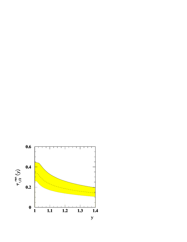
VII Numerical results

The numerical analysis of the sum rule for $\tau_{1/2}$ can be carried out using the same input parameters adopted in Sect.IV for the determination of $F^{+}$. In particular, we use the explicit expressions of the two-point sum rules determining the leptonic constants $F^{+}$ and $F$ that appear in the pole contribution of eq.(19). We vary the threshold parameters in the ranges $\nu_{c}=2-3$ GeV and $\nu^{\prime}_{c}=2.5-3.5$ GeV, obtaining an acceptable stability window, where the results do not appreciably depend on the Borel parameters, in the ranges around $\tau\simeq 1.5$ GeV and $\tau^{\prime}\simeq 2$ GeV, respectively. The contribution of the nonperturbative term in the three-point correlator represents a small fraction of the total contribution; on the other hand, the $\alpha_{s}$ correction in the perturbative term is sizeable, but it turns out to be partially compensated by the analogous correction in the leptonic constants $F$ and $F^{+}$. Notice that this is a remarkable result, not expected a priori since the normalization of the form factor, for example at zero recoil, is not fixed by symmetry arguments. The perturbative corrections, however, do not equally affect the form factor for all values of the variable $y$, but they are sensibly $y-$dependent, with the effect of increasing the slope of $\tau_{1/2}$ with respect to the case where they are omitted.

The results for $\tau_{1/2}^{ren}(y)$ are shown in fig.3, where the curves refer to various choices for the continuum thresholds. The region limited by the curves essentially determines the theoretical accuracy allowed by the present calculation.

Considering the $y$ dependence, the limited range of values allowed by the mass difference between $D$ and $D_{0}$ permits the expansion near $y=1$:

$$\tau_{1/2}^{ren}(y)=\tau_{1/2}(1)\Big{(}1-\rho^{2}_{1/2}(y-1)+c_{1/2}(y-1)^{2}\Big{)}\;\;\;.$$ (126)

A two-parameter fit to fig.3, in terms of the normalization at zero recoil and the slope, gives $\tau_{1/2}(1)=0.31\pm 0.06$ and $\rho^{2}_{1/2}=1.5\pm 0.4$. The inclusion of the quadratic term modifies the fit as follows:

$$\tau_{1/2}(1)=0.35\pm 0.08\;\;,\hskip 28.45274pt\rho^{2}_{1/2}=2.5\pm 1.0\;\;,\hskip 28.45274ptc_{1/2}=3\pm 3$$ (127)

which is the result we quote for our analysis.

The immediate application of this result concerns the prediction of the semileptonic $B$ decay rates to $D_{0}$ and $D_{1}^{*}$. Using $V_{cb}=3.9\times 10^{-2}$ and $\tau(B)=1.56\times 10^{-12}$ sec, we obtain

$${\cal B}(B\to D_{0}\ell\bar{\nu})=(5\pm 3)\times 10^{-4}\hskip 28.45274pt{\cal B}(B\to D^{*}_{1}\ell\bar{\nu})=(7\pm 5)\times 10^{-4}\;\;\;.$$ (128)

This means that only a very small fraction of the semileptonic $B\to X_{c}$ decays is represented by transitions into the $s_{\ell}^{P}={1\over 2}^{+}$ charmed doublet. Although small, however, one cannot exclude that such processes will be identified, mainly at dedicated $B$-facilities which will be running in the near future. At present, the measurements of semileptonic $B\to D^{**}$ decays only provide data on the members of the $s_{\ell}^{P}={3\over 2}^{+}$ doublet [45, 46], since the doublet with $s_{\ell}^{P}={1\over 2}^{+}$ is not distinguished from the non-resonant charmed background. In particular, in [45] the $B$ semileptonic branching fraction to the final states $D\pi$ and $D^{*}\pi$ of $(20\pm 5)\;10^{-2}$ is reported.

VIII Conclusions

We conclude observing that HQET has proven to be a powerful tool to handle heavy quark physics. However, predictions derived in this framework should always be supported by the computation of $1/m_{Q}$ as well as radiative corrections. The role of both depend on the specific situation one is facing with. For example, they turn out to be important for the $B$ meson leptonic constant, while they are moderate for the Isgur-Wise function, as derived in [12]. We have presented here the case of the universal form factor $\tau_{1/2}(y)$ describing $B$ semileptonic transitions to the excited $J^{P}=(0^{+},1^{+})$ charmed states, using QCD sum rules in the framework of HQET. As already shown in [12], the computation of loop integrals results to be greatly simplified within HQET. The task of computing perturbative corrections to $\tau_{1/2}(y)$ is justified by manifold interesting phenomenological features of orbitally excited states as well as by the many theoretical interests already mentioned. We have obtained a situation similar to the case of the Isgur-Wise function, namely radiative corrections are quite under control for $\tau_{1/2}(y)$, while they affect considerably the value of the leptonic constant $F^{+}$ of the $s_{\ell}=1/2$ doublet.

A Parametric Integrals

The calculation of the two-loop diagrams relevant for the form factor $\tau_{1/2}$ essentially follows the analogous calculation for the Isgur-Wise function [12], with the main difference represented by the need of keeping different Borel parameters, due to the non-symmetric nature of the problem at hand. We only recall here that, in momentum space, the Feynman rules of HQET [3, 4, 5] can be reduced to the heavy quark propagator ${\not\!v\,+1\over 2}{i\over v\cdot k}$, and to the heavy-quark-gluon vertex $ig_{s}v_{\mu}{\lambda^{a}\over 2}$; $N_{c}$ is the number of colours and $Tr[{\lambda^{a}\over 2}{\lambda^{a}\over 2}]=C_{F}={N_{c}^{2}-1\over 2N_{c}}$.

The calculation of the loop integrals is performed in $D=4+2\epsilon$ Euclidean space-time dimensions. The main ingredients are the representations of the propagators of the massless quark and of the heavy quark:

$${1\over(s_{E}^{2})^{a}} = {\Gamma\Big{(}{D\over 2}-a\Big{)}\over\pi^{D/2}\Gamma(a)}\int d^{D}x{e^{2is_{E}\cdot x}\over(x^{2})^{D/2-a}}$$ (A1)

$${1\over(\omega+2iv_{E}\cdot s_{E})^{\alpha}} = {(-1)^{\alpha}\over\Gamma(\alpha)}\int_{0}^{\infty}d\lambda\lambda^{\alpha-1}e^{\lambda(\omega+2iv_{E}\cdot s_{E})}$$ (A2)

($v_{E},s_{E}$ obtained from the four-vectors $v,s$ by a Wick rotation); in particular, (A2) is useful for the computation of the integrals after Borel transformation, since

$${\hat{B}}^{(\omega)}_{\tau}e^{\lambda\omega}=\delta(\lambda-\tau^{-1})\;\;\;.$$ (A3)

The master integrals needed in the evaluation of the loop integrals can be found in [47, 44]. Here we report a number of parametric integrals useful for the calculation of the Borel-transformed expressions $\hat{D}_{1}-\hat{D}_{6}$:

$$F_{1}(z) = \int_{0}^{1}{du\over V^{2}(uz)}=-{1\over 2z\sqrt{y^{2}-1}}\;\ln\Big{[}{y_{+}+z\over y_{+}^{2}(y_{-}+z)}\Big{]}\;,$$ (A4)

$$F_{2}(z) = V^{2}(z)\int_{0}^{1}{du\over\Big{[}V^{2}(uz)\Big{]}^{2}}={1\over 2(y^{2}-1)}[y(y+z)+y^{2}-1-V^{2}(z)F_{1}(z)]\;,$$ (A5)

$$F_{4}(z) = V^{2}(z)\int_{0}^{1}du{\ln(1-u)\over\Big{[}V^{2}(uz)\Big{]}^{2}}=-{1\over 2}F_{1}(z)-\ln{V^{2}(z)}\Big{(}1+{y\over z}\Big{)}{1\over 4(y^{2}-1)}$$ (A6)

$$+ V^{2}(z){1\over 4z(y^{2}-1)}\Big{[}{\cal L}(y,z)+{1\over z}\ln{V^{2}(z)}F_{1}\Big{(}{1\over z}\Big{)}-z\ln{V^{2}\Big{(}{1\over z}\Big{)}}F_{1}(z)\Big{]}\;,$$ (A7)

$$F_{5}(z) = \int_{0}^{1}du{\ln{V^{2}(uz)}\over V^{2}(uz)}$$ (A8)

$$= -{1\over z}h(y,z)-{1\over z^{2}}F_{1}\Big{(}{1\over z}\Big{)}\ln{V^{2}(z)}+\sqrt{y^{2}-1}F_{1}(z)\Big{[}r(y)+{1\over z}F_{1}\Big{(}{1\over z}\Big{)}\Big{]}\;,$$ (A9)

$$F_{6}(z) = V^{2}(z)\int_{0}^{1}du{\ln{V^{2}(uz)}\over\Big{[}V^{2}(uz)\Big{]}^{2}}={V^{2}(z)\over 2(y^{2}-1)}\Bigg{\{}F_{1}(z)-F_{5}(z)+{y\over z}-{\Big{(}{y\over z}+1\Big{)}\over V^{2}(z)}[1+\ln{V^{2}(z)}]\Bigg{\}}\;,$$ (A10)

$$F_{7}(z) = \int_{0}^{1}du{\ln(1-u)\over 1-u}\Bigg{[}{[V^{2}(z)]^{2}\over[V^{2}(uz)]^{2}}-1\Bigg{]}=(y+z)zF_{4}(z)\Big{[}1-{2(y^{2}-1)\over V^{2}(z)}\Big{]}$$ (A11)

$$- {z\over 2}(y+z)F_{1}(z)\Big{[}1+{2(y^{2}-1)\over V^{2}(z)}\Big{]}-{1\over 4}\ln{V^{2}(z)}\Big{[}3+{2(y^{2}-1)\over V^{2}(z)}\Big{]}+{1\over 4}\ln{V^{2}(z)}\ln{V^{2}\Big{(}{1\over z}\Big{)}}$$ (A12)

$$- (y^{2}-1)F_{1}(z)F_{1}\Big{(}{1\over z}\Big{)}-{\pi^{2}\over 6}+{1\over 2}{\cal L}_{1}(y,z)\;,$$ (A13)

$$F_{8}(z) = [V^{2}(z)]^{2}\int_{0}^{1}{du\over 1-u}{\ln{V^{2}(uz)}-\ln{V^{2}(z)}\over[V^{2}(uz)]^{2}}=-{\cal L}_{1}\Big{(}y,{1\over z}\Big{)}-{1\over 4}\big{[}\ln{V^{2}(z)}\big{]}^{2}$$ (A14)

$$- (y+z)\ln{V^{2}(z)}zF_{1}(z)-{1\over 2}+{1\over 2}V^{2}(z)\big{[}1-\ln{V^{2}(z)}\big{]}$$ (A15)

$$+ z(y+z)\big{[}F_{5}(z)+F_{6}(z)-\ln{V^{2}(z)}F_{2}(z)\big{]}\;,$$ (A16)

$$F_{9}(z) = \int_{0}^{1}{du\over 1-u}\Bigg{[}{[V^{2}(z)]^{2}\over[V^{2}(uz)]^{2}}-1\Bigg{]}=z(y+z)\big{[}F_{1}(z)+F_{2}(z)\big{]}+{\big{[}\ln{V^{2}(z)}+V^{2}(z)-1\big{]}\over 2}\;.$$ (A17)

In $F_{1}-F_{8}$ the combinations have been introduced:

$$h(y,z) = {1\over\sqrt{y^{2}-1}}\Bigg{[}-L_{2}(1-y_{-}^{2})+L_{2}\Big{(}{y_{+}(1-y_{-}^{2})\over y_{+}+z}\Big{)}\Bigg{]}\;,$$ (A18)

$${\cal L}(y,z) = {1\over\sqrt{y^{2}-1}}\Bigg{[}L_{2}\Big{(}{1\over 1+y_{-}z}\Big{)}-L_{2}\Big{(}{1\over 1+y_{+}z}\Big{)}\Bigg{]}\;,$$ (A19)

$${\cal L}_{1}(y,z) = L_{2}\Big{(}{1\over 1+y_{-}z}\Big{)}+L_{2}\Big{(}{1\over 1+y_{+}z}\Big{)}\;,$$ (A20)

where $L_{2}(x)$ is the dilogarithm. The integrals $F_{1}(z)-F_{9}(z)$ coincide with those reported in [12] for $z=1$. Finally, a useful identity needed in the calculation of $D_{5}^{(3)}$, $D_{6}^{(3)}$ is

$${\cal L}\Big{(}y,{\tau\over\tau^{\prime}}\Big{)}-{\cal L}\Big{(}y,{\tau^{\prime}\over\tau}\Big{)}=-{\tau^{\prime}\over\tau}F_{1}\Big{(}{\tau^{\prime}\over\tau}\Big{)}\ln{V^{2}\Big{(}{\tau\over\tau^{\prime}}\Big{)}}+{\tau\over\tau^{\prime}}F_{1}\Big{(}{\tau\over\tau^{\prime}}\Big{)}\ln{V^{2}\Big{(}{\tau^{\prime}\over\tau}\Big{)}}\;.$$ (A21)

FIGURE CAPTIONS

Fig. 1

Binding energy parameter $\bar{\Lambda}^{+}$ and leptonic constant $F^{+}_{ren}$ of the doublet $s_{\ell}^{P}={1\over 2}^{+}$, from the QCD sum rule analysis of the correlator eq.(26). The curves refer to three choices of the threshold parameter $\nu^{\prime}_{c}$: $\nu^{\prime}_{c}=2.5$ GeV (continuous line), $\nu^{\prime}_{c}=3.0$ GeV (dashed line), $\nu^{\prime}_{c}=3.5$ GeV (dotted line).

Fig. 2

Two-loop diagrams relevant for the calculation of ${\cal O}(\alpha_{s})$ corrections to the perturbative part of the QCD sum rule for the form factor $\tau_{1/2}$. The heavy lines represent the heavy quark propagators in HQET.

Fig. 3

The universal form factor $\tau_{1/2}^{ren}(y)$. The curves refer to choices of the threshold parameters: $\nu_{c}=2.0$ GeV, $\nu^{\prime}_{c}=2.5$ GeV (continuous line), $\nu_{c}=2.5$ GeV, $\nu^{\prime}_{c}=3.0$ GeV (dashed line), $\nu_{c}=3.0$ GeV, $\nu^{\prime}_{c}=3.5$ GeV (dotted line).

FIG. 1.:

FIG. 2.:

FIG. 3.:

REFERENCES

• [1] N. Isgur and M.B. Wise, Phys.Β Lett. B 232, 113 (1989); 237, 527 (1990).
• [2] M.B. Voloshin and M.A. Shifman, Yad.Β Fiz.Β 45, 463 (1987) [Sov.Β J.Β Nucl.Β Phys.Β 45, 292 (1987)]; 47, 801 (1988) [47, 511 (1988)].
• [3] E. Eichten and B. Hill, Phys. Lett. B 234, 511 (1990); 243, 427 (1990). H. Georgi, Phys. Lett. B 240, 447 (1990). T. Mannel, W. Roberts and Z. Ryzak, Nucl. Phys. B 368, 204 (1992).
• [4] A.F. Falk, H. Georgi, B. Grinstein and M.B. Wise, Nucl. Phys. B 343, 1 (1990).
• [5] For reviews on HQET see e.g.: H. Georgi, ”Heavy Quark Effective Field Theory” Proceedings of the Boulder TASI, (1991) page 589; B. Grinstein, ”An Introduction to Heavy Mesons”, Proceedings of the 6th Mexican School of Particles and Fields, Villahermosa, Mexico, 3-7 Oct 1994, page 122; M. Neubert, ”Heavy Quark Effective Theory”, Proceedings of the International School of Subnuclear Physics: 34th Course: Effective Theories and Fundamental Interactions, Erice, Italy, 3-12 Jul 1996, page 98.
• [6] M. A. Shifman, A. I. Vainshtein and V. I. Zakharov, Nucl. Phys. B 147, 385 (1979); B 147, 448 (1979). For a review on the QCD sum rule method see: ”Vacuum structure and QCD Sum Rules”, edited by M. A. Shifman, North-Holland, 1992.
• [7] M. Neubert, Phys. Rept. 245, 259 (1994).
• [8] D.J. Broadhurst and A.G. Grozin, Phys.Β Lett. B 274, 421 (1992).
• [9] M. Neubert, Phys. Rev. D 45, 2451 (1992).
• [10] E. Bagan, P. Ball, V.M. Braun and H. G. Dosch, Phys.Β Lett. B 278, 457 (1992).
• [11] For a recent review of lattice QCD results on heavy meson systems see, e.g., J.M. Flynn and C.T. Sachrajda, report SHEP-97-20, to appear in Heavy Flavours (2nd ed.), eds. A.J. Buras and M. Lindner (World Scientific, Singapore) (hep-lat/9710057).
• [12] M. Neubert, Phys. Rev. D 47, 4063 (1993).
• [13] E. Bagan, P. Ball and P. Gosdzinsky, Phys. Lett. B 301, 249 (1993).
• [14] M. Neubert, Z. Ligeti and Y. Nir, Phys. Lett. B 301, 101 (1993); Phys. Rev. D 47, 5060 (1993). M. Neubert, Nucl. Phys. B 416, 786 (1994).
• [15] M. Neubert, in Proceedings of the 17th International Symposium of Lepton Photon Interactions, Beijing (China) Aug. 10-15, 1995, Eds. Z. Z.-Peng and C. He-Sheng, World Scientific (1996), p. 298.
• [16] N. Isgur and M.B. Wise, Phys. Rev. D 43, 819 (1991).
• [17] J.D. Bjorken, Proceedings of the 4th Rencontres de Physique de la VallΓ©e d’Aoste, La Thuile, Italy, 1990, edited by M. Greco, (Editions FrontiΓ¨res, Gif sur Yvette, 1990) page 583.
• [18] M.B. Voloshin, Phys. Rev. D 46, 3062 (1992).
• [19] For a review see: I. Bigi, M. Shifman and N.G. Uraltsev, Ann. Rev. Nucl. Part. Sci. 47, 591 (1997).
• [20] A.K. Leibovich, A. Ligeti, J.W. Steward and M. B. Wise, Phys. Rev. Lett. 78, 3995 (1997); Phys. Rev. D 57, 308 (1998).
• [21] P. Colangelo, F. De Fazio and G. Nardulli, Phys. Lett. B 303, 152 (1993). G. Lopez Castro and J. H. Munoz, Phys. Rev. D 55, 5581 (1997). M. Neubert, Phys. Lett. B 418, 173 (1998).
• [22] J. Charles et al., report LPTHE-ORSAY-97-70, hep-ph/9801363.
• [23] J.L. Rosner, Comm. Nucl. Part. Phys. 16, 109 (1986). S. Balk, J.G. KΓΆrner, G. Thomson and F. Hussain, Zeit. Phys. C 59, 283 (1993).
• [24] Review of Particle Properties, R.M. Barnett et al., Phys. Rev. D 54, 1 (1996).
• [25] P. Abreu et al., DELPHI Collab., Phys. Lett. B 345, 598 (1995). R. Akers et al., OPAL Collab., Z. Phys. C 66, 19 (1995). D. Buskulic et al., ALEPH Collab., Z. Phys. C 69 393 (1996).
• [26] A.F. Falk and M. Luke, Phys. Lett. B 292, 119 (1992).
• [27] P. Colangelo et al., Phys. Rev. D 52, 6422 (1995). P. Colangelo and F. De Fazio, hep-ph/9706271, to appear in European Physical Journal C - Particles and Fields.
• [28] U. Kilian, J.G. KΓΆrner and D. Pirjol, Phys. Lett. B 288, 360 (1992).
• [29] X. Ji and M.J. Musolf, Phys. Lett. B 257, 409 (1991). G.P. Korchemsky and A.V. Radyushkin, Nucl. Phys. B 283, 342 (1987). G.P. Korchemsky, Mod. Phys. Lett. A 4, 1257 (1989).
• [30] P. Colangelo, G. Nardulli and N. Paver, Phys. Lett. B 293, 207 (1992). P. Colangelo, G. Nardulli, A.A. Ovchinnikov and N. Paver, Phys. Lett. B 269, 204 (1991).
• [31] T.B. Suzuki, T. Ito, S. Sawada and M. Matsuda, Prog. Theor. Phys. 91, 757 (1994).
• [32] A. Wambach, Nucl. Phys. B 434, 647 (1995).
• [33] S. Veseli and M.G. Olsson, Phys. Lett. B 367 302, (1996); Z. Phys. C 71 287, (1996); Phys. Rev. D 54 886, (1996).
• [34] V. Morenas et al., Phys. Rev. D 56 5668, (1997).
• [35] A. Deandrea et al., report CPT-98-P-3620 (February 1998).
• [36] Y.B. Dai, C.S. Huang, M.Q. Huang and C. Liu, Phys. Lett. B 390, 350 (1997). Y.B. Dai, C.S. Huang and M.Q. Huang, Phys. Rev. D 55, 5719 (1997).
• [37] Y.B. Dai, C.S. Huang, M.Q. Huang, H.Y. Jin and C. Liu, hep-ph/9705223.
• [38] V. Morenas et al., report LPTHE 97-23, PCCF RI 9708, hep-ph/9710298.
• [39] S. Veseli and I. Dunietz, Phys. Rev. D 54, 6803 (1996). S. Godfrey and N. Isgur, Phys. Rev. D 32, 189 (1985). P. Colangelo, G. Nardulli and M. Pietroni, Phys. Rev. D 43, 3002 (1991).
• [40] N. Isgur, D. Scora, B. Grinstein and M. B. Wise, Phys. Rev. D 39, 799 (1989).
• [41] F.V. Tkachov, Phys.Β Lett.Β B 100, 65 (1981). K.G. Chetyrkin and F.V. Tkachov, Nucl.Β Phys.Β B 192, 159 (1981). D.I. Kazakov, Phys.Β Lett.Β B 133, 406 (1983). N. Gray et al., Z.Β Phys.Β C 48, 673 (1990).
• [42] A. V. Kotikov, Phys. Lett. B 254, 158 (1991); 259, 314 (1991).
• [43] H.D. Politzer and M.B. Wise, Phys.Β Lett.Β B 206, 681 (1988); 208, 504 (1988).
• [44] D.J. Broadhurst and A.G. Grozin, Phys.Β Lett.Β B 267, 105 (1991).
• [45] D. Buskulic et al., ALEPH Collaboration, Z. Phys. C 73, 601 (1997).
• [46] A. Anastassov et al., CLEO Collaboration, report CLNS-97-1501, hep-ex/9708035.
• [47] M. Neubert, Phys.Β Rev.Β D 46, 1076 (1992); 46, 3914 (1992).