Solving a Coupled Set of Truncated QCD Dyson–Schwinger Equations

Abstract

Truncated Dyson–Schwinger equations represent finite subsets of the equations of motion for Green’s functions. Solutions to these non–linear integral equations can account for non–perturbative correlations. A closed set of coupled Dyson–Schwinger equations for the propagators of gluons and ghosts in Landau gauge QCD is obtained by neglecting all contributions from irreducible 4–point correlations and by implementing the Slavnov–Taylor identities for the 3–point vertex functions. We solve this coupled set in an one–dimensional approximation which allows for an analytic infrared expansion necessary to obtain numerically stable results. This technique, which was also used in our previous solution of the gluon Dyson–Schwinger equation in the Mandelstam approximation, is here extended to solve the coupled set of integral equations for the propagators of gluons and ghosts simultaneously. In particular, the gluon propagator is shown to vanish for small spacelike momenta whereas the previoulsy neglected ghost propagator is found to be enhanced in the infrared. The running coupling of the non–perturbative subtraction scheme approaches an infrared stable fixed point at a critical value of the coupling, $\alpha_{c}\simeq 9.5$.

PACS Numbers: 02.30Rz 11.15.Tk 12.38.Aw 14.70.Dj

UNITU–THEP–3/1998 FAU–TP3–98/2

, ,

PROGRAM SUMMARY

Title of program: gluonghost

Catalogue identifier:

Program obtainable from: CPC Program Library, Queen’s University of Belfast, N. Ireland

Computers: Workstation DEC Alpha 500

Operating system under which the program has been tested: UNIX

Programming language used: Fortran 90

Memory required to execute with typical data: 200 kB

No. of bits in a word: 32

No. of processors used: 1

Has the code been vectorized of parallelized?: No

Peripherals used: standard output, disk

No. of lines in distributed program, including test data, etc.: 247

Distribution format: ASCII

Keywords:
Non–perturbative QCD, Dyson–Schwinger equations, gluon and ghost propagator, Landau gauge, Mandelstam approximation, non–linear integral equations, infrared asymptotic series, constrained iterative solution.

Nature of physical problem:
One non–perturbative approach to non–Abelian gauge theories is to investigate their Dyson-Schwinger equations in suitable truncation schemes. For the pure gauge theory, i.e., for gluons and ghosts in Landau gauge QCD without quarks, such a scheme is derived in Ref. [1]. In numerical solutions one generally encounters non–linear, infrared singular sets of coupled integral equations.

Method of solution:
The singular part of the integral equations is treated analytically and transformed into constraints extending our previous work [2] to a coupled system of equations. The solution in the infrared is then expanded into an asymptotic series which together with the known ultraviolet behavior makes a numerical solution tractable.

Restrictions on the complexity of the problem:
Solving the coupled system of Dyson–Schwinger equations relies on a modified angle approximation to reduce the 4–dimensional integrals to one–dimensional ones.

Typical running time: One minute

LONG WRITE-UP

1 The physical problem

1.1 Introduction

The infrared regime of non–Abelian gauge theories is inaccessible to perturbation theory. Confinement, being a long–distance effect, is expected to manifest itself in the infrared behavior of the Green’s functions of the theory. Thus, in solving truncated sets of Dyson–Schwinger equations (DSEs) in order to determine the propagators self–consistently, infrared singularities have to be anticipated. This implies some special precautions in the numerical problem.

In this paper we present the numerical solution of the coupled gluon and ghost DSEs in which the infrared behavior of the corresponding propagators is determined analytically. In particular, asymptotic series for their infrared structure are calculated recursively prior to the iterative process. The DSEs being non–linear integral equations these series represent a systematic formulation of the consistency requirements in the extreme infrared on possible solutions. The method of simultaneously expanding the solutions to a coupled set of equations generalizes the one used in Ref. [1] where only the gluon propagator was considered in an approximation in which ghost contributions are omitted [2, 3, 4].

This paper is organized as follows: In the next subsection we summarize the truncation scheme used in order to arrive at a closed system of equations. In the following subsection the reduction to one–dimensional integral equations is presented. For completeness we give also the most important steps of the renormalization procedure. In section two the numerical method is discussed with special emphasis on the semi–analytic solutions in the infrared as well as in the ultraviolet. The numerical method based on iteration for intermediate momenta and matching to analytic expressions for small and large momenta is explained. Numerical results are presented and some implications of their infrared behavior are discussed. For more details in the derivation of the truncation scheme and for a further discussion of the physical implications of the results we refer the reader to Refs. [5, 6].

1.2 A solvable truncation scheme

In order to keep this paper self–contained we first summarize the trunctation scheme used to arrive at a closed system of equations [5].

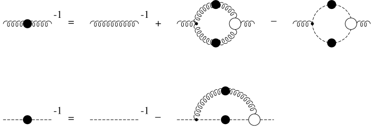
For simplicity we consider the pure gauge theory and neglect all quark contributions. In addition to the elementary two–point functions, the ghost and gluon propagators, the Dyson–Schwinger equation for the gluon propagator also involves the three– and four–point vertex functions which obey their own Dyson–Schwinger equations. These equations involve successive higher n–point functions. The used truncation of the gluon equation includes to neglect all terms with four–gluon vertices. These are the momentum independent tadpole term, an irrelevant constant which vanishes perturbatively in Landau gauge, and explicit two–loop contributions to the gluon DSE. The renormalized equation for the inverse gluon propagator in Euclidean momentum space with positive definite metric, $g_{\mu\nu}=\delta_{\mu\nu}$, (color indices suppressed) is then given by

$$D^{-1}_{\mu\nu}(k)=Z_{3}\,{D^{\text{tl}}}^{-1}_{\mu\nu}(k)-g^{2}N_{c}\,\widetilde{Z}_{1}\int\frac{d^{4}q}{(2\pi)^{4}}\;iq_{\mu}\,D_{G}(p)\,D_{G}(q)\,G_{\nu}(q,p)\\ +g^{2}N_{c}\,Z_{1}\frac{1}{2}\int\frac{d^{4}q}{(2\pi)^{4}}\;\Gamma^{\text{tl}}_{\mu\rho\alpha}(k,-p,q)\,D_{\alpha\beta}(q)D_{\rho\sigma}(p)\,\Gamma_{\beta\sigma\nu}(-q,p,-k)\;,$$ (1)

where $p=k+q$, $D^{\text{tl}}$ and $\Gamma^{\text{tl}}$ are the tree–level propagator and three–gluon vertex, $D_{G}$ is the ghost propagator and $\Gamma$ and $G$ are the fully dressed 3–point vertex functions. The DSE for the ghost propagator in Landau gauge QCD, without any truncations, is given by

$$D_{G}^{-1}(k)=-\widetilde{Z}_{3}\,k^{2}+g^{2}N_{c}\,\widetilde{Z}_{1}\int\frac{d^{4}q}{(2\pi)^{4}}\;ik_{\mu}\,D_{\mu\nu}(k-q)\,G_{\nu}(k,q)\,D_{G}(q)\;.$$ (2)

The coupled set of equations for the gluon and ghost propagator, eqs. (1) and (2), is graphically depicted in Fig. 1. The renormalized propagators for ghosts and gluons, $D_{G}$ and $D$, and the renormalized coupling $g$ are defined from the respective bare quantities by introducing multiplicative renormalization constants,

$$\widetilde{Z}_{3}D_{G}:=D^{0}_{G}\;,\quad Z_{3}D_{\mu\nu}:=D^{0}_{\mu\nu}\;,\quad Z_{g}g:=g_{0}\;.$$ (3)

In Landau gauge, which we adopt in the following, one has $\widetilde{Z}_{1}=Z_{g}Z_{3}^{1/2}\widetilde{Z}_{3}=1$ and $Z_{1}=Z_{g}Z_{3}^{3/2}$. The $SU(N_{c}=3)$ structure constants $f^{abc}$ of the gauge group (and the coupling $g$) are separated from the 3–point vertex functions by defining:

Figure 1: Diagrammatic representation of the gluon and ghost Dyson–Schwinger equations in the truncation scheme applied in this paper.

$$\Gamma^{abc}_{\mu\nu\rho}(k,p,q)=gf^{abc}(2\pi)^{4}\delta^{4}(k+p+q)\Gamma_{\mu\nu\rho}(k,p,q)\;.\quad\hbox{ \begin{minipage}[c]{108.405pt} \psfig{width=390.25534pt} \end{minipage}}$$ (4)

The arguments of the 3–gluon vertex denote the three incoming gluon momenta according to its Lorentz indices (counter clockwise starting from the dot). With this definition, the tree–level vertex has the form,

$$\Gamma^{\text{tl}}_{\mu\nu\rho}(k,p,q)=-i(k-p)_{\rho}\delta_{\mu\nu}-i(p-q)_{\mu}\delta_{\nu\rho}-i(q-k)_{\nu}\delta_{\mu\rho}\;.$$ (5)

The arguments of the ghost–gluon vertex are the outgoing and incoming ghost momenta respectively,

$$G^{abc}_{\mu}(p,q)=gf^{abc}G_{\mu}(p,q)\;.\qquad\hbox{ \begin{minipage}[c]{108.405pt} \psfig{width=346.89731pt} \end{minipage}}$$ (6)

Note that the color structure of all three loop diagrams in Fig. 1 is simply given by $f^{acd}f^{bdc}=-N_{c}\delta^{ab}$ which was used in Eqs. (1) and (2) suppressing the trivial color structure of the propagators $\sim\delta^{ab}$.

The ghost and gluon propagators in Landau gauge are parameterized by their respective renormalization functions $G$ and $Z$,

$$D_{G}(k) =-\frac{G(k^{2})}{k^{2}}\qquad\text{and}$$ (7)

$$D_{\mu\nu}(k) =\frac{Z(k^{2})}{k^{2}}\left(\delta_{\mu\nu}-{k_{\mu}k_{\nu}\over k^{2}}\right)\;.$$ (8)

In order to obtain a closed set of equations for the functions $G$ and $Z$ the ghost–gluon and the 3–gluon vertex functions have to be specified. We construct these vertex functions from their respective Slavnov–Taylor identities (STIs) as entailed by the Becchi–Rouet–Stora (BRS) symmetry. In particular, in Ref. [5] we derive the STI of the gluon–ghost vertex from BRS invariance. Neglecting irreducible ghost rescattering, an assumption fully compatible with the present truncation scheme, this new identity together with the symmetry properties of the vertex constrain the full structure of the gluon–ghost vertex which expressed in terms of the ghost renormalization function reads [5]:

$$G_{\mu}(p,q)=iq_{\mu}\,\frac{G(k^{2})}{G(q^{2})}+ip_{\mu}\,\biggl{(}\frac{G(k^{2})}{G(p^{2})}-1\biggr{)}\;.$$ (9)

At the same time, this gluon–ghost vertex implies a rather simple form for a ghost–gluon scattering kernel of tree–level structure which in turn allows for a straightforward resolution of the STI for the 3–gluon vertex [5]. Neglecting some unconstrained terms which are transverse with respect to all three gluon momenta the solution for the 3–gluon vertex follows from the general constructions in Refs. [7, 8, 9]. As a result, the 3–gluon vertex can again be expressed in terms of the gluon and ghost renormalization functions [5]:

$$\Gamma_{\mu\nu\rho}(p,q,k)=-A_{+}(p^{2},q^{2};k^{2})\,\delta_{\mu\nu}\,i(p-q)_{\rho}-A_{-}(p^{2},q^{2};k^{2})\,\delta_{\mu\nu}\,i(p+q)_{\rho}\\ -2\frac{A_{-}(p^{2},q^{2};k^{2})}{p^{2}-q^{2}}(\delta_{\mu\nu}pq-p_{\nu}q_{\mu})\,i(p-q)_{\rho}\,+\text{cyclic permutations}\;,$$ (10)

with

$$A_{\pm}(p^{2},q^{2};k^{2})=\frac{G(k^{2})}{2}\,\left(\frac{G(q^{2})}{G(p^{2})Z(p^{2})}\pm\frac{G(p^{2})}{G(q^{2})Z(q^{2})}\right)\quad.$$ (11)

This establishes a closed system of equations for the renormalization functions $G(k^{2})$ and $Z(k^{2})$ of ghosts and gluons, which consists of their respective DSEs (1) and (2) using the vertex functions (9) and (10/11). Thereby explicit 4–gluon vertices (in the gluon DSE (1)) as well as irreducible 4–ghost correlations (in the identity for the ghost–gluon vertex) and non–trivial contributions from the ghost–gluon scattering kernel (to the Slavnov–Taylor identity for the 3–gluon vertex) were neglected. Since, at present, we do not attempt to solve this system in its full 4–dimensional form (but in a one–dimensional approximation), we refer the reader to Ref. [5] for its explicit form.

1.3 The modified angle approximation

In this section, illustrated at the example of the less complex ghost DSE, we present the approximation used to render the integral equations one–dimensional. This especially allows for a thorough discussion of their infrared and ultraviolet asymptotic behavior, which is a necessary prerequisite to stable numerical results. The leading order of the integrands in the infrared limit of integration momenta is hereby preserved. Furthermore, the correct short distance behavior of the solutions (obtained at high integration momenta) is also unaffected. From (2) with the vertex (9) we obtain the following equation for the ghost renormalization function $G(k^{2})$,

$$\frac{1}{G(k^{2})}=\widetilde{Z}_{3}-g^{2}N_{c}\int\frac{d^{4}q}{(2\pi)^{4}}\,\biggl{(}k\mathcal{P}(p)q\biggr{)}\,\frac{Z(p^{2})G(q^{2})}{k^{2}\,p^{2}\,q^{2}}\\ \times\left(\frac{G(p^{2})}{G(q^{2})}+\frac{G(p^{2})}{G(k^{2})}-1\right)\;,\quad p=k-q\;,$$ (12)

where $\mathcal{P}^{\mu\nu}(p)=\delta^{\mu\nu}-p^{\mu}p^{\nu}/p^{2}$ is the transversal projector. In order to perform the integration over the 4–dimensional angular variables analytically, we make the following approximation:

For $q^{2}>k^{2}$ we assume that the functions $Z$ and $G$ are slowly varying with their arguments and that we are thus allowed to replace $G(p^{2})\simeq G(k^{2})\to G(q^{2})$. This assumption ensures the correct leading ultraviolet behavior of the equation according to the resummed perturbative result at one–loop level [5]. For all momenta being large, i.e. in the perturbative limit, this approximation is well justified by the slow logarithmic momentum dependence of the perturbative renormalization functions for ghosts and gluons. Our solutions will resemble this behavior, justifying the validity of the approximation in this limit. Note that previously this same assumption was used for arbitrary integration momenta $q^{2}$ in the derivation of the one–dimensional equation for the gluon renormalization function in Mandelstam approximation [1, 2, 3, 4]. In this case, in particular for small $q^{2}<k^{2}$, the infrared enhanced solution tends to invalidate this assumption.

For $q^{2}<k^{2}$ we therefore proceed with an angle approximation instead, which preserves the limit $q^{2}\to 0$ of the integrands replacing the arguments of the functions $Z$ and $G$ according to $G(p^{2})=G((k-q)^{2})\to G(k^{2})$ and $Z(p^{2})\to Z(k^{2})$. In this form, the one–dimensional approximation was used in a very recent investigation of the coupled system of ghost and gluon DSEs using only tree–level vertices [10]. However, using this approximation for arbitrary $q^{2}$ (in particular also for $q^{2}>k^{2}$ as in Ref. [10]) one does not recover the renormalization group improved one–loop results for asymptotically large momenta.

We therefore use that particular version of the two different one–dimensional approximations that is appropriate for the respective cases, $q^{2}\lessgtr k^{2}$. In this modified angle approximation, we obtain from (12) upon angular integration,

$$\frac{1}{G(k^{2})}=\widetilde{Z}_{3}-\frac{g^{2}}{16\pi^{2}}\frac{3N_{c}}{4}\left(\frac{1}{2}\,Z(k^{2})G(k^{2})+\int_{k^{2}}^{\Lambda^{2}}\frac{dq^{2}}{q^{2}}\,Z(q^{2})G(q^{2})\right)\;,$$ (13)

where we introduced an $O(4)$–invariant momentum cutoff $\Lambda$ to account for the logarithmic ultraviolet divergence, which will have to be absorbed by the renormalization constant.

It has several advantages (summarized in Ref. [5]) to use the projector

$$\mathcal{R}_{\mu\nu}(k)=\delta_{\mu\nu}-4\,\frac{k_{\mu}k_{\nu}}{k^{2}}\quad,$$ (14)

in the gluon DSE to isolate a scalar equation for $Z(k^{2})$ from Eq. (1). With the same one–dimensional reduction as used for the ghost DSE we obtain

$$\frac{1}{Z(k^{2})}=Z_{3}+Z_{1}\frac{g^{2}}{16\pi^{2}}\frac{N_{c}}{3}\left\{\int_{0}^{k^{2}}\frac{dq^{2}}{k^{2}}\left(\frac{7}{2}\frac{q^{4}}{k^{4}}-\frac{17}{2}\frac{q^{2}}{k^{2}}-\frac{9}{8}\right)Z(q^{2})G(q^{2})\right.\\ +\left.\int_{k^{2}}^{\Lambda^{2}}\frac{dq^{2}}{q^{2}}\left(\frac{7}{8}\frac{k^{2}}{q^{2}}-7\right)Z(q^{2})G(q^{2})\right\}\\ +\frac{g^{2}}{16\pi^{2}}\frac{N_{c}}{3}\left\{\int_{0}^{k^{2}}\frac{dq^{2}}{k^{2}}\frac{3}{2}\frac{q^{2}}{k^{2}}G(k^{2})G(q^{2})-\frac{1}{3}G^{2}(k^{2})+\frac{1}{2}\int_{k^{2}}^{\Lambda^{2}}\frac{dq^{2}}{q^{2}}G^{2}(q^{2})\right\}\;.$$ (15)

In the derivation of Eq. (15), however, we omitted one contribution from the 3–gluon loop for $q^{2}<k^{2}$, namely the following term:

$$-\frac{g^{2}Z_{1}N_{c}}{6}\!\!\int_{q^{2}<k^{2}}\!\!\frac{d^{4}q}{(2\pi)^{4}}\,N(p^{2},q^{2};k^{2})\left(\frac{Z(p^{2})G(p^{2})}{G(q^{2})}-\frac{Z(q^{2})G(q^{2})}{G(p^{2})}\right)\frac{G(k^{2})}{k^{2}\,p^{2}\,q^{2}}$$ (16)

with

$$N(x,y;z)=\frac{5x^{3}+41x^{2}y+5xy^{2}-3y^{3}}{4x(y-x)}+\frac{x^{2}-10xy+24y^{2}}{2(y-z)}\\ +\frac{x^{3}+9x^{2}y-9xy^{2}-y^{3}}{xz}+\frac{(2x^{2}+11xy-3y^{2})z}{2x(x-y)}+\frac{(x+y)z^{2}}{4x(y-x)}\;.$$ (17)

Due to the singularity in $N(p^{2},q^{2};k^{2})$ for $p^{2}\to q^{2}$ which has to be cancelled from the terms in brackets, this contribution would generate an artificial singularity if the angle approximation was applied. We will assess the influence of this term below in order to justify its omission.

The only difference in the 3–gluon loop as obtained here versus the Mandelstam approximation (see [1]) is that the gluon renormalization function $Z$ is replaced by the product $ZG$. The system of equations (13) and (15) is a direct extension to the gluon DSE in the Mandelstam approximation [1]. Thus, the methods developed for solving the Mandelstam equation have to be generalized to solve the coupled Eqs. (13) and (15).

It will furthermore become clear shortly that the leading infrared behavior of the solutions is unaffected by the additional manipulation to the 3–gluon loop. This was also confirmed in Ref. [10] where the same qualitative behavior of the solutions in the infrared was obtained neglecting the 3–gluon loop completely.

With the Ansatz that for $x:=k^{2}\to 0$ the product $Z(x)G(x)\to cx^{\kappa}$, the ghost DSE (13) with $N_{c}=3$ yields,

$$G(x) \to\left(g^{2}\frac{9}{64\pi^{2}}\left(\frac{1}{\kappa}-\frac{1}{2}\right)\right)^{-1}c^{-1}x^{-\kappa}\;,$$ (18)

$$Z(x) \to\left(g^{2}\frac{9}{64\pi^{2}}\left(\frac{1}{\kappa}-\frac{1}{2}\right)\right)\,c^{2}x^{2\kappa}\;.$$ (19)

Furthermore, in order to obtain a positive definite function $G(x)$ for positive $x$ from a positive definite $Z(x)$, as $x\to 0$, we find the necessary condition $1/\kappa-1/2>0$ which is equivalent to

$$0<\kappa<2\;.$$ (20)

The special case $\kappa=0$ leads to a logarithmic singularity in Eq. (13) for $x\to 0$. In particular, assuming that $ZG=c$ with some constant $c>0$ and $x<x_{0}$ for a sufficiently small $x_{0}$, we obtain $G^{-1}(x)\to c\,(9g^{2}/64\pi^{2})\,\ln(x/x_{0})+\text{const}$ and thus $G(x)\to 0^{-}$ for $x\to 0$, showing that no positive definite solution can be found in this case either.

It is important to note that the ghost–loop gives infrared singular contributions $\sim x^{-2\kappa}$ to the gluon equation (15) while the 3–gluon loop yields terms proportional to $x^{\kappa}$ as $x\to 0$, which are thus subleading contributions to the gluon equation in the infrared. With Eq. (18) the leading asymptotic behavior of Eq. (15) for $x\to 0$ leads to

$$Z(x)\to g^{2}\frac{9}{64\pi^{2}}\,\frac{9}{4}\left(\frac{1}{\kappa}-\frac{1}{2}\right)^{2}\left(\frac{3}{2}\,\frac{1}{2-\kappa}-\frac{1}{3}+\frac{1}{4\kappa}\right)^{-1}\,c^{2}x^{2\kappa}\;.$$ (21)

Consistency between (19) and (21) requires that

$$\left(\frac{3}{2}\,\frac{1}{2-\kappa}-\frac{1}{3}+\frac{1}{4\kappa}\right)\,\stackrel{{\scriptstyle!}}{{=}}\,\frac{9}{4}\left(\frac{1}{\kappa}-\frac{1}{2}\right)\;.$$ (22)

Using the constraint (20) in addition, the solution is given uniquely by

$$\kappa=\frac{61-\sqrt{1897}}{19}\simeq 0.92\;.$$ (23)

From these considerations alone we can conclude that the leading behavior of the gluon and ghost renormalization functions and thus their propagators in the infrared is entirely due to ghost contributions. The details of the treatment of the 3–gluon loop have no influence on the above considerations. This is in remarkable contrast to the Mandelstam approximation, in which the 3–gluon loop alone determines the infrared behavior of the gluon propagator and the running coupling in Landau gauge [1, 2, 3, 4]. On the other hand, the present picture is confirmed by the ghost–loop only approximation to the coupled gluon and ghost DSEs which yields the same qualitative infrared behavior as investigated in Ref. [10]. The quantitative discrepancy in their numerical value for the exponent $\kappa\simeq 0.77$ can be attributed to their using of tree–level vertices as compared to the STI improvements used here. In contrast to the infrared, however, the 3–gluon loop is crucial for the correct anomalous dimensions which determine the leading behavior of the propagators in the ultraviolet.

1.4 Renormalization

In Landau gauge the renormalization constants (as introduced in Eq. (3)) obey the identity [11]:

$$\widetilde{Z}_{1}=Z_{g}Z_{3}^{1/2}\widetilde{Z}_{3}=1\;.$$ (24)

The Slavnov–Taylor identity for the ghost–gluon vertex ensures that this remains valid also in general covariant gauges as long as irreducible 4–ghost correlations are neglected [5]. In the following we will exploit the implication of Eq. (24), namely that the product $g^{2}Z(k^{2})G^{2}(k^{2})$ is renormalization group invariant. Near the ultraviolet fixed point this invariant is identified with the running coupling. Non–perturbatively, though there is no unique (scheme independent) way of defining a running coupling, invariance under arbitrary renormalization group transformations $(g,\mu)\to(g^{\prime},\mu^{\prime})$ allows the identification

$$g^{2}Z({\mu^{\prime}}^{2})G^{2}({\mu^{\prime}}^{2})\stackrel{{\scriptstyle!}}{{=}}{g^{\prime}}^{2}=\bar{g}^{2}(\ln({\mu^{\prime}}/\mu),g)\;.$$ (25)

This being one of the conditions that fix the non–perturbative subtraction scheme, it yields a physically sensible definition of a non–perturbative running coupling in pure Landau gauge QCD [5]. Note that this identification of the non–perturbative running coupling is an extension to the procedure we used in the Mandelstam approximation [1]. In this approximation without ghosts the identity $Z_{g}Z_{3}=1$ implies that $gZ(k^{2})$ is the corresponding renormalization group invariant product which is replaced by $g^{2}ZG^{2}$ in presence of ghosts.

The one–dimensional DSEs (13) and (15) can actually be cast in an explicitly scale independent form using the following Ansatz to parameterize the functions $G$ and $Z$ motivated from their one–loop scaling behavior:

$$Z(k^{2}) =\left(\frac{F(x)}{F(s)}\right)^{1-2\delta}\,R^{2}(x)\;,$$ (26)

$$G(k^{2}) =\left(\frac{F(x)}{F(s)}\right)^{\delta}\,\frac{1}{R(x)}\quad\text{with}\quad x:=k^{2}/\sigma\quad\text{and}\quad s:=\mu^{2}/\sigma\;,$$

where $\sigma$ is some currently unfixed renormalization group invariant scale parameter and $\delta=9/44$. From the definition of the running coupling (25) we find that $\bar{g}^{2}(t_{k},g)\sim F(x)$ with $t_{k}=\frac{1}{2}\ln k^{2}/\mu^{2}$. We fix the constant of proportionality for later convenience by setting (with $\beta_{0}=11N_{c}/(48\pi^{2})$ for $N_{f}=0$ quark flavors),

$$\beta_{0}\,\bar{g}^{2}(t_{k},g)=F(x)\quad\text{and}\quad\alpha_{S}(\mu)=\frac{g^{2}}{4\pi}=\frac{1}{4\pi\beta_{0}}\,F(s)\;.$$ (27)

The fact that from the resulting equations besides the running coupling $F(x)$ also the second function $R(x)$ turns out to be independent on the renormalization scale $s$ shows that the solutions to the renormlized DSEs for ghosts and gluons formally obey one–loop scaling at all scales [5]. The non–perturvative nature of the result thus is entirely contained in the running coupling.

As the infrared behavior of the solutions $G$ and $Z$, Eqs. (18) and (19) respectively, can be extracted without actually solving the DSEs, we find for the running coupling accordingly,

$$g^{2}Z(k^{2})G^{2}(k^{2})=\bar{g}^{2}(t_{k},g)\,\stackrel{{\scriptstyle t_{k}\to-\infty}}{{\longrightarrow}}\,\left(\frac{9}{64\pi^{2}}\left(\frac{1}{\kappa}-\frac{1}{2}\right)\right)^{-1}=:\,g_{c}^{2}\;.$$ (28)

With Eq. (23) for $\kappa$ we obtain $g_{c}^{2}\simeq 119.1$ which corresponds to a critical coupling $\alpha_{c}=g^{2}_{c}/(4\pi)\simeq 9.48$. This is in clear contrast to the running coupling obtained in the Mandelstam approximation [1]. The dynamical inclusion of ghosts changes the infrared singular coupling of the Mandelstam approximation to an infrared finite one implying the existence of an infrared stable fixed point.

With the parameterization (26) and setting $k^{2}=\mu^{2}$ ($\Leftrightarrow x=s$) with $\beta_{0}g^{2}=F(s)$ we obtain equations for the renormalization constants $Z_{3}$ and $\widetilde{Z}_{3}$. For the latter, this can immediately be used to eliminate $\widetilde{Z}_{3}$ from the ghost DSE which then reads [5],

$$\frac{R(x)}{F^{\delta}(x)}=\frac{9}{44}\int_{0}^{x}\frac{dy}{y}\,R(y)F^{1-\delta}(y)-\frac{9}{88}\,R(x)F^{1-\delta}(x)\;.$$ (29)

The gluon DSE (15) for $x=s$ contains the additional renormalization constant of the 3–gluon vertex $Z_{1}$ which is a divergent quantity in perturbation theory since in Landau gauge $Z_{1}=Z_{3}/\widetilde{Z}_{3}\sim(g^{2}/g_{0}^{2})^{1-3\delta}$. It turns out that the corresponding (one–loop) renormalization scale dependence of this constant is needed in the DSE for the solution to reproduce the correct scale dependence asymptotically. Not so, however, a possible cutoff dependence of $Z_{1}$ (from $g_{0}^{2}$) which cannot be removed from equation (15) consistently [5]. Substituting in $Z_{1}$ the cutoff scale by the integration momentum $y$ by using $Z_{1}=(F(s)/F(y))^{1-3\delta}$ takes care of the scale dependence of $Z_{1}$ without introducing an additional divergence. While this manipulation leads to the correct scaling limit for the gluon propagator [5], it might give indications towards possible improvements on the truncation and approximation scheme. It also allows to remove the gluon renormalization constant $Z_{3}$ from Eq. (15) and the same steps as for the ghost equation yield,

$$\frac{11}{R^{2}(x)F^{1-2\delta}(x)}=\int_{0}^{x}\frac{dy}{x}\,\left(\frac{7}{2}\frac{y^{2}}{x^{2}}-\frac{17}{2}\frac{y}{x}-\frac{9}{8}+7\frac{x}{y}\right)R(y)F^{2\delta}(y)\\ +x\frac{7}{8}\,\int_{x}^{\infty}\frac{dy}{y^{2}}\,R(y)F^{2\delta}(y)+\frac{3}{2}\,\frac{F^{\delta}(x)}{R(x)}\int_{0}^{x}\frac{dy}{x}\frac{y}{x}\,\frac{F^{\delta}(y)}{R(y)}-\frac{1}{3}\frac{F^{2\delta}(x)}{R^{2}(x)}\\ -\frac{1}{2}\int_{0}^{x}\frac{dy}{y}\,\left(\frac{F^{2\delta}(y)}{R^{2}(y)}-\frac{1}{4\kappa}\,\frac{a^{2\delta}}{b^{2}y^{2\kappa}}\right)+\frac{1}{4\kappa}\,\frac{a^{2\delta}}{b^{2}x^{2\kappa}}\;,$$ (30)

where $\kappa$ is the exponent (23). Furthermore, $a:=\beta_{0}g_{c}^{2}=F(0)$ and $b$ is defined through the leading infrared behavior of $R(x)\to bx^{\kappa}$ for $x\to 0$.

2 Numerical methods

2.1 Asymptotic series in the infrared and behavior in the ultraviolett

Eqs. (29) and (30) do not depend on the renormalization scale $s=\mu^{2}/\sigma$. This implies that the functions $F(x)$ and $R(x)$ are renormalization group invariant. In particular, the scaling behavior of the propagators follows trivially from the solution for the non–perturbative running coupling.

Following the method used to obtain our previous solution to the gluon DSE in Mandelstam approximation we are going to expand the functions $F(x)$ and $R(x)$ in the infrared in terms of asymptotic series. Due to the nature of the coupled set of equations a recursive calculation of the respective coefficients is considerably more difficult than in Mandelstam approximation [3, 1]. For $x<x_{0}$ where $x_{0}$ is some infrared matching point, the asymptotic series to at least next–to–leading order is used in obtaining iterative solutions for $x>x_{0}$. The matching point $x_{0}$ has to be sufficiently small for the asymptotic series to provide the desired accuracy. On the other hand, limited by numerical stability, it cannot be chosen arbitrarily small either. This leads to a certain range of values of $x_{0}$ for which stable solutions are obtained with no matching point dependence to fixed accuracy. The additional inclusion of the next–to–next–to–leading order contributions in the asymptotic series has no effect other than increasing the allowed range for the matching point as we will show below.

We proceed further by noting that the equation for the ghost propagator, Eq. (29), can be converted into a first order homogeneous linear differential equation for $R(x)$ by differentiating Eq. (29) with respect to $x$:

$$R^{\prime}(x)=\frac{\delta}{1+\frac{\delta}{2}F}\,\left(\frac{F}{x}+\frac{F^{\prime}}{F}-\frac{1-\delta}{2}F^{\prime}\right)\;R(x)\;.$$ (31)

The gluon equation, Eq. (30) can be rewritten as

$$\frac{11}{R^{2}(x)F^{1-2\delta}(x)}=\int_{0}^{x}\frac{dy}{x}\,\Bigg{\{}\left(\frac{7}{2}\frac{y^{2}}{x^{2}}-\frac{17}{2}\frac{y}{x}-\frac{9}{8}+7\frac{x}{y}-\frac{7}{8}\frac{x^{2}}{y^{2}}\right)R(y)F^{2\delta}(y)\\ +\frac{7}{8}\frac{x^{2}}{y^{2}}\,ba^{2\delta}\,y^{\kappa}\Bigg{\}}+\frac{7}{8}\frac{b\,a^{2\delta}}{1-\kappa}\,x^{\kappa}+A\,x+\frac{3}{2}\,\frac{F^{\delta}(x)}{R(x)}\int_{0}^{x}\frac{dy}{x}\frac{y}{x}\,\frac{F^{\delta}(y)}{R(y)}\\ -\frac{1}{3}\frac{F^{2\delta}(x)}{R^{2}(x)}-\frac{1}{2}\int_{0}^{x}\frac{dy}{y}\,\left(\frac{F^{2\delta}(y)}{R^{2}(y)}-\frac{1}{4\kappa}\,\frac{a^{2\delta}}{b^{2}y^{2\kappa}}\right)+\frac{1}{4\kappa}\,\frac{a^{2\delta}}{b^{2}x^{2\kappa}}\;,$$ (32)

where we have used that

$$x\frac{7}{8}\,\int_{x}^{\infty}\frac{dy}{y^{2}}\,R(y)F^{2\delta}(y)=-x\frac{7}{8}\,\int_{0}^{x}\frac{dy}{y^{2}}\left(RF^{2\delta}-ba^{2\delta}y^{\kappa}\right)+\frac{7}{8}\frac{b\,a^{2\delta}}{1-\kappa}\,x^{\kappa}\,+A\,x\\ \text{with}\quad A=\frac{7}{8}\,\int_{0}^{\infty}\frac{dy}{y^{2}}\left(RF^{2\delta}-b\,a^{2\delta}y^{\kappa}\right)\;.$$ (33)

It follows from the leading infrared behavior, i.e., $F\to a$ and $R\to bx^{\kappa}$ for $x\to 0$, and Eq. (29) that an asymptotic infrared expansion of the l.h.s. of Eq. (32) has to contain powers of $x^{\kappa}$ as well as integer powers of $x$ in subsequent subleading terms. This motivates the following Ansatz,

$$R(x) =b\,x^{\kappa}\sum_{l,m,n=0}^{l+m+n=N}C_{lmn}\;x^{m\nu+3n\kappa+l(1+2\kappa)}$$ (34)

$$F(x) =a\,\sum_{l,m,n=0}^{l+m+n=N}D_{lmn}\;x^{m\nu+3n\kappa+l(1+2\kappa)}\;,$$ (35)

with $C_{000}=D_{000}=1$. The terms proportional to $x^{\nu}$ in these expansions are allowed to find the most general subleading behavior compatible with the consistency in the infrared. Below we will see that $\nu\simeq 2.05$. Using $2<3\kappa<1+2\kappa\lesssim 3$ one finds that different orders in this expansions do not mix in their successive importance at small $x$. Furthermore the leading infrared contributions are analytically evaluated and explicitly subtracted from all integrals, assuming that the remaining contributions are integrable for $x\to 0$. For the subleading contributions to $R$ and $F$ suppressed by powers of $x^{\nu}$ with $\nu\simeq 2.05$ this is justified a posteriori.

Inserting the series (34) and (35) into Eq. (31) allows to relate the coefficients $C_{lmn}$ to $D_{lmn}$. In the solution of Eq. (31) the integration constant is set to $b$. In the order $N=1$ one thus obtains:

$$C_{100} =\left(\frac{\kappa(1-3\kappa)}{2(1+2\kappa)}+\delta\right)D_{100}$$

$$C_{010} =\left(\frac{\kappa}{\nu}-\frac{\kappa}{2}-\frac{\kappa^{2}}{2\nu}+\delta\right)D_{010}$$ (36)

$$C_{001} =\left(\frac{1}{3}-\frac{2}{3}\kappa+\delta\right)D_{001}\;.$$

At higher orders in $N$ this procedure recursively yields relations that uniquely determine the coefficients $C_{lmn}$ in terms of the coefficients $D_{lmn}$. Further relations are obtained from Eq. (32) by expanding all ratios of $R$ and $F$ which occur with dependence on $x$ and $y$, and by comparison of the respective orders, $\mathcal{O}(x^{m\nu+(3n-2)\kappa+l(1+2\kappa)})$ on both sides. To leading order $N=0$,i.e., $\mathcal{O}(x^{-2\kappa})$, from Eq. (32) one obtains

$$\frac{11}{b^{2}\,a^{1-2\delta}}=\left(\frac{3}{2}\,\frac{1}{2-\kappa}-\frac{1}{3}+\frac{1}{4\kappa}\right)\,\frac{a^{2\delta}}{b^{2}}\;.$$ (37)

With $a=\beta_{0}g_{c}^{2}=((9/44)(1/\kappa-1/2))^{-1}$ this is nothing more than our previously used Eq. (23) which determines $\kappa$. At order $N=1$ Eq. (32) yields

$$\hskip-28.45274pt\mathcal{O}(x^{\nu-2\kappa}):\hskip 28.45274pt\frac{11}{a}\left(D_{010}+2(C_{010}-\delta D_{010})\right)=$$

$$\left(\frac{3}{2}\left(\frac{1}{2+\nu-\kappa}+\frac{1}{2-\kappa}\right)-\frac{2}{3}-\frac{1}{\nu-2\kappa}\right)(C_{010}-\delta D_{010})$$ (38)

$$\hskip-28.45274pt\mathcal{O}(x^{\kappa}):\hskip 42.67912pt\frac{11}{a}\left(D_{001}+2(C_{001}-\delta D_{001})\right)=-b^{3}f(\kappa)+$$

$$\left(\frac{3}{2}\left(\frac{1}{2+2\kappa}+\frac{1}{2-\kappa}\right)-\frac{2}{3}-\frac{1}{\kappa}\right)(C_{001}-\delta D_{001})$$ (39)

$$\hskip-28.45274pt\mathcal{O}(x):\hskip 48.36958pt\frac{11}{a}\left(D_{100}+2(C_{100}-\delta D_{100})\right)=-\frac{b^{2}}{a^{2\delta}}\,A\,+$$

$$\left(\frac{3}{2}\left(\frac{1}{3+\kappa}+\frac{1}{2-\kappa}\right)-\frac{5}{3}\right)(C_{100}-\delta D_{100})\;,$$ (40)

with

$$f(\kappa):=\frac{7}{2(3+\kappa)}-\frac{17}{2(2+\kappa)}-\frac{9}{8(1+\kappa)}+\frac{7}{\kappa}+\frac{7}{8(1-\kappa)}\;.$$ (41)

Eqs. (36) and (38)–(41) determine the coefficients $D$ and $C$ to lowest non–trivial order. They decouple into three times two equations for each pair $(C_{lmn},D_{lmn})$. For $(l,m,n)=(1,0,0)$ one obtains

$$C_{100}\simeq 0.05554b^{2}A\quad\text{and}\quad D_{100}\simeq-0.6992b^{2}A\;,$$ (42)

where the constant $A$ is defined in Eq. (33) The set of equations for $(l,m,n)=(0,1,0)$, Eqs. (38)–(41), is homogeneous. The determinant of its 2–dimensional coefficient matrix is zero for

$$\nu=\frac{-6-\kappa-3\kappa^{2}\pm\sqrt{\left(3+2\kappa\right)\left(104+92\kappa\right)\kappa^{2}+\left(6+\kappa+3\kappa^{2}\right)^{2}}}{2\left(3+2\kappa\right)}\;.$$ (43)

There exists one positive root for the plus sign which determines the positive exponent $\nu$. With $\kappa=(61-\sqrt{1897})/19$ one arrives at

$$\nu\simeq 2.051\quad\hbox{and}\quad C_{010}=-0.0124D_{010}\;.$$ (44)

For $(l,m,n)=(0,0,1)$ the scale of the coefficients is set by the inhomogeneity in Eq. (39), $b^{3}f(\kappa)$, yielding

$$C_{001}\,\simeq\,1.969\,b^{3}\;,\quad\hbox{and}\quad D_{001}\,\simeq\,-26.52\,b^{3}\;.$$ (45)

Based on these next–to–leading order results, higher orders, though increasingly tedious, can be obtained recursively by analogous sets of equations. The general pattern is such that the lower order fixes the scales for higher order coefficients. This allows to define scale independent coefficients $\widetilde{C}$ and $\widetilde{D}$ by extracting their respective scales according to the exponent $\tau_{lmn}=m\nu+3n\kappa+l(1+2\kappa)$ of $x$ for a given set $(l,m,n)$,

$$C_{lmn}=:\widetilde{C}_{lmn}\,b^{3n+2l}\,t^{m}\,A^{l}\;,\quad\text{and}\quad D_{lmn}=:\widetilde{D}_{lmn}\,b^{3n+2l}\,t^{m}\,A^{l}\;.$$ (46)

The scale of the powers of $x^{\nu}$ is set by $D_{010}$ and we have defined for convenience

$$t:=-D_{010}$$ (47)

i.e., $\widetilde{C}_{010}\simeq 0.0124$ and $\widetilde{D}_{010}=-1$. We summarize the values of the coefficients $\widetilde{C}$ and $\widetilde{D}$ for $N=2$ in table 1.

$(l,m,n)$	$(2,0,0)$	$(1,1,0)$	$(1,0,1)$	$(0,2,0)$	$(0,1,1)$	$(0,0,2)$
$\widetilde{C}$	-0.1042	-0.3034	-7.933	-0.2160	-11.55	-151.0
$\widetilde{D}$	0.5246	1.590	40.10	1.226	60.98	766.8

Table 1: Coefficients of the asymptotic expansion for $N=2$.

The two parameters $b$ and $t$ are related to the overall momentum scale. After fixing the scale one is still left with one independent parameter. This leads to a scale invariance which can be described as follows: A change in the momentum scale $\sigma$ (introduced by $x=k^{2}/\sigma$) according to $\sigma\to\sigma^{\prime}=\sigma/\lambda$ or, equivalently, $x\to x^{\prime}=\lambda x$ can be compensated by

$$b\,\to\,b^{\prime}=b/\lambda^{\kappa}\;,\quad\text{and}\quad t\,\to\,t^{\prime}=t/\lambda^{\nu}\;.$$ (48)

We choose the scale without loss of generality such that the positive number $b=1$. The parameter $t$ can in principle be any real number including zero. We can find numerically stable iterative solutions for not too large absolute values of $t$ (see below). Furthermore, it can be verified numerically, that a solution for a value of $b\not=1$ for fixed $t$ is identical to a solution for $b=1$ and $t^{\prime}=t\,b^{\nu/\kappa}$, if $x$ is substituted by $x^{\prime}=x/b^{1/\kappa}$. This is the numerical manifestation of the scale invariance mentioned above (for $\lambda=1/b^{1/\kappa}$). Note that under scale transformations (48) the constant $A$ appearing in Eq. (33) trivially transforms according to its dimension, $A\to A^{\prime}=A/\lambda$, without any adjustments from the way it is calculated:

$$A^{\prime}=A/\lambda=\lim_{x_{0}^{\prime}\to 0}\,\frac{7}{8}\left(\int_{x_{0}^{\prime}}^{\infty}\frac{dy^{\prime}}{{y^{\prime}}^{2}}\,R(y^{\prime})F^{2\delta}(y^{\prime})-b^{\prime}a^{2\delta}\frac{(x_{0}^{\prime})^{\kappa-1}}{1-\kappa}\right)\;.$$ (49)

Figure 2: The numerical solutions of $F(x)$ and $R(x)$ for $t=0$ and $b=1$ together with their asymptotic expansions to order $N=1$ as well as $N=2$ at small $x$.

In Fig. 2 the numerical solutions for $F(x)$ and $R(x)$ for $b=1$ and $t=0$ at small $x$ together with their respective asymptotic forms to order $N=1$ and $N=2$ are displayed. The contributions of the order $N=2$ in the asymptotic expansion become comparable in size to the lower order at about $x\simeq 0.2$. As the error in the asymptotic series is of the order of the first terms neglected, this supplies an estimate for the range of $x$ in which the asymptotic expansion can yield reliable results. In the particular calculation described below we used a value of about $x_{0}=0.01$ for the matching point relating the result of the iterative process to the asymptotic expansion. This is obviously well below the estimated range of the validity of the asymptotic expansion.

As already stated, for intermediate momenta the integral is done numerically. In the ultraviolet limit, i.e. for $x\to\infty$, we have $F(x)\to 1/\ln x$ and $R(x)\to 1$ which allows us to alleviate the cut–off dependence in the numerical determination of $A$. Note that this is the only integral left with the upper boundary being infinity. In Eq. (33) the corresponding integral is calculated using an ultraviolet matching point $x_{1}$ and

$$\int_{x_{1}}^{\infty}dx\frac{RF^{2\delta}}{x^{2}}\quad\longrightarrow\quad\int_{x_{1}}^{\infty}dx\frac{1}{x^{2}(\ln x)^{2\delta}}=\Gamma(1-2\delta,\ln x_{1})$$ (50)

for sufficiently large $x_{1}$, where $\Gamma(a,x)$ is the incomplete gamma function.

Similarly to the case of Mandelstam’s approximation [1] we calculated all integrals using a Simpson integration routine of fourth order. In order to reduce the numerical errors which can otherwise destroy the convergence we had to use meshpoints equidistant on a logarithmic scale, i.e.,

$$\int dy\longrightarrow\int du\,y\quad\text{with}\quad u=\ln y\quad.$$ (51)

Convergence properties are furthemore significantly improved by weighting the iteration: Instead of a full update of the functions with every step we introduced an exponentially distributed weight between the two functions,

$$\eta=\frac{1}{2}\text{e}^{-(\Delta_{F}+\Delta_{R})/2}\;,$$ (52)

where $\Delta_{F}$ is defined by

$$\Delta_{F}:=\max\{|\tilde{F}_{i+1}(j)/F_{i}(j)-1|\}_{j}\;,$$ (53)

and with an analogous definition of $\Delta_{R}$. Here, $\tilde{F}_{i+1}$ is the preliminary result of the $i$th iteration step calcualted using the input $F_{i}$ as obtained from the previous iteration. From this, the input for the subsequent iteration is choosen not to be the full new $\tilde{F}_{i+1}$ but rather

$$F_{i+1}=(1-\eta)\tilde{F}_{i+1}+\eta F_{i}\;,\quad\text{and}\quad R_{i+1}=(1-\eta)\tilde{R}_{i+1}+\eta R_{i}\;$$ (54)

analogously. This increases the stability of the algorithm by suppressing possible oszillations in the iteration.

2.2 Numerical results

Most of the numerical results reported here were obtained with the order $N=1$ in the asymptotic expansion. We checked explicitely for all cases that no dependence on the matching point exists for $0.01\leq x_{0}\leq 0.1$ We have calculated $F$ and $R$ for several values in the range $-5\leq t\leq 16$. At lower negative values the procedure became numerically unstable due to a developing (tachyonic) pole in $F(x)$. The fact that the integral equations for $R$ and $F$ possess a one–parameter family of solutions characterized by $t$ is in fact the reason for the necessity of the infrared expansion up to next to leading order. No stable solution can be found numerically without fixing the leading $x$–dependence of $F(x)$ at small $x$ by choosing a value for the parameter $t$. This is a boundary condition to be imposed on the solutions from physical arguments.

Figure 3: The numerical solutions of $F(x)$ and $R(x)$ with $b=1$ for different values of the parameter $t=\{-4,-2,-1,0,1,2,4,8,16\}$ (solid lines represent $t=0$ solutions).

In Fig. 3 the numerical results are displayed for different values of the parameter $t$ (all with $b=1$). Perturbatively, we expect $R(x)$ to approach a constant value and $F(x)\to 1/\ln(\lambda x)$ for $x\to\infty$. The reason we introduced here the constant $\lambda$ in the one–loop running coupling $F$ is that we fixed the momentum scale in our calculations by arbitrarily setting $b=1$. The relation between the scale of perturbative QCD $\Lambda_{\text{QCD}}$ and $\sigma$ cannot be determined this way. Therefore, we set $\Lambda^{2}_{\hbox{\tiny QCD}}=\sigma/\lambda$ for some scale parameter $\lambda$. Fixing the scale in our calculations from the phenomenological value of $\alpha_{S}$ at the mass of the $Z$–boson, one obtains $\sigma\simeq(350\text{MeV})^{2}$ for the $t=0$ solution for $F$. A detailed discussion of the anomalous dimensions of gluons and ghosts allows an estimate of $\lambda$ to be in the range $1.5\sim 2$ which corresponds to a $\Lambda_{\text{QCD}}$ in $250\sim 300$MeV [5]. The solutions for $t\not=0$ display a qualitatively similar behavior at high momenta with slightly different values. The solutions for positive values of $t$ seem to have more residual momentum dependence in $R$ at high momenta than those for $t\leq 0$. For negative values of $t$ the running coupling, $\alpha_{S}(\mu)=F(s)/(4\pi\beta_{0})$, has a maximum, $\alpha_{\text{max}}>\alpha_{c}$, at a finite value of the renormalization scale $s=\mu^{2}/\sigma$. This is because the dominant subleading term of the running coupling in the infrared is determined by $t$,

$$F(x)\to a(1-tx^{\nu}+D_{001}x^{3\kappa}+D_{100}x^{1+2\kappa})\;,\quad x\to 0\;.$$ (55)

With $\nu\simeq 2.05<3\kappa<1+2\kappa$ and $D_{001}<0$, it is clear that for $t<0$ the running coupling increases for smallest scales close to $\mu=0$ before higher order terms dominate. There necessarily has to be a maximum $\alpha_{\text{max}}>\alpha_{c}$ at some finite scale $\mu$ for any solution with $t<0$.

For $t\geq 0$, $\alpha_{c}=\alpha(\mu=0)$ is the only maximum of the running coupling for all real values of the renormalization scale, and $\alpha_{c}$ is thus a true infrared stable fixed point. Comparing the behavior of the resulting gluon and ghost renormalization functions in the ultraviolet we observe that, for the $t\geq 0$ solutions, the case $t=0$ yields the best resemblance of their one–loop anomalous dimensions. We therefore interpret the case $t=0$ as the most physical one and conceive the existence of solutions for $t\not=0$ as a mathematical peculiarity.

In reducing the DSE for the gluon propagator to a one–dimensional equation we had to dismiss the contribution (16) in order to avoid an artificial singular contribution. To asses whether this is justified we calculate the contribution from (16) without the one–dimensional approximation from the gluon and ghost renormalization functions as obtained from the iterative scheme, i.e., from the one–dimensional integral equations. In Fig. 4 the inverse gluon function is displayed as a measure of the terms retained on the r.h.s. of the one–dimensional equation (15). This is to be compared to the neglected contribution (16) as calculated from the selfconsistent results. One clearly observes that the dismissed contribution remains small at all momenta and becomes negligible for small and large momenta quickly. Although, in principle, even small contributions might become important in non–linear self–consistency problems this is rather convincing support for the omission of the terms in (16) to which the one–dimensional approximation cannot be applied.

Figure 4: The dismissed contribution (16) compared to the inverse gluon function.

3 Conclusions

We have solved a set of two coupled non–linear integral equations. These solutions involve functions which are highly singular in the infrared. The corresponding infrared behavior has to be treated analytically by converting the integral equations into recursion relations for the coefficients of asymptotic expansions. The final numerical solution is obtained by matching the asymptotic expansions to an iteration process used for momenta above the matching point.

The numerical algorithm described here was used in the solution of the coupled gluon–ghost Dyson–Schwinger equations reported in Refs. [5, 6] for the first time. The resulting gluon and ghost propagators displayed a new type of infrared behavior involving irrational exponents of the momenta. This generic type of DSE solutions for gluon and ghost propagators of the same qualitative form has been verified recently using a different truncation scheme and different numerical methods [10]. We therefore believe that the algorithm presented here will prove useful in further studies of Dyson–Schwinger equations also.

4 Description of the program

4.1 The main program

After defining the variables and setting the parameters $\kappa,\nu,a$ etc. and the matching points $x_{0}$ and $x_{1}$ the functions $F(x)$ and $R(x)$ are initialized to

$$F(x)=\frac{1}{\ln(1.1+x)}\quad\text{and}\quad R(x)=1+(x-1)\text{e}^{-x}\;.$$ (56)

The iteration process consists of several parts. The first is the evaluation of the constant $A$ (see (33) and (50)) using the functions determined in the previous iteration step. Hereby Eq. (50) is used for large momenta. Next, the contributions to the gluon and ghost equations due to the infrared region is calculated using the expansion in the asymptotic series. In the intermediate momentum range the integrals above the infrared matching point are computed numerically with the help of an Simpson routine of fourth order using the mesh defined by Eq. (51). Application of Eqs. (52) to (54) completes the iteration step.

Convergence is tested by comparing the input and output functions of an iteration step pointwise. If the maximum relative deviation is less than EPS it is assumed that convergence is achieved, and the result is written to the file gluonghost.out in three-column form: $x,F(x),R(x)$.

4.2 Subroutines and functions

Function Simpson
Returns the integral of a function which is given at equally spaced abscissas. As far as the number of abscissas is sufficient this function uses a closed Simpson rule of order $1/N^{4}$ [13].

Function Gamma
This routine returns the incomplete gamma function $\Gamma(a,x)$ using a continued fraction as described in [13].

5 Testing the program

Naturally, trivial tests establishing the independence of the number of meshpoints, the infrared matching point $x_{0}$, the ultraviolet cut-off $x_{1}$ and the order of the asymptotic series in the infrared have been performed. We could also verify that the results are independent of the initializing functions chosen at the beginning.

TEST RUN

standard output

Number of meshpoints :  500
Infrared matching point :  0.01
Ultraviolet cut-off :  1.0E+08
parameter t =  0.0
eps =  1.0E-07

Convergence achieved after 126 iterations!
max. deviation between Fin and Fout:  9.47201E-08
max. deviation between Rin and Rout:  3.42583E-08
Output written to gluonghost.out

gluonghost.out

    0.1000000000E-01    0.8298109605E+01    0.1457629245E-01
    0.1047128548E-01    0.8297891961E+01    0.1520601418E-01
    0.1096478196E-01    0.8298096464E+01    0.1586253844E-01
                              ...
    0.9120108394E+08    0.6234215822E-01    0.9295472468E+00
    0.9549925860E+08    0.6218344927E-01    0.9296193060E+00
    0.1000000000E+09    0.6202552418E-01    0.9296910980E+00