KEK-TH-568

hep-ph/9804327

April 1998

1 Introduction

Processes mediated by flavor changing neutral current (FCNC) have been considered as good probes of physics beyond the standard model (SM). By using the experimentally well measured processes, it is expected to obtain an indirect evidence or constraints on new physics models. An existence of new physics may arise as violation of the unitarity of the Cabbibo-Kobayashi-Maskawa (CKM) matrix. Such signatures of new physics will be explored through the determination of the unitarity triangle at B-factories at KEK and SLAC in the near future.

Typical FCNC processes which have been often used to study the new physics contributions are $B^{0}\mbox{-}\overline{B^{0}}$ and $K^{0}\mbox{-}\overline{K^{0}}$ mixings. Parameters $x_{d}$ in $B^{0}\mbox{-}\overline{B^{0}}$ mixing and $\epsilon_{K}$ in $K^{0}\mbox{-}\overline{K^{0}}$ mixing are dominated by the short distance physics and have been calculated in the SM and many new physics models. Experimentally, both parameters have been measured as [1]

$$x_{d} = 0.73\pm 0.05,$$ (1.1a)

$$|\epsilon_{K}| = (2.23\pm 0.013)\times 10^{-3}.$$ (1.1b)

On the other hand, there are large theoretical uncertainties on both parameters which come from the evaluation of the hadronic matrix elements of those processes. They are parametrized in terms of decay constants and bag-parameters of $B$ or $K$ mesons. Thus, the loss of information on the CKM matrix elements or the new physics contributions from those processes is not avoidable in the level of these uncertainties.

The rare decay $K^{+}\rightarrow\pi^{+}\nu\overline{\nu}$ is one of the most promising processes to extract clean informations about the CKM matrix elements [2] because the decay rate of this process has small theoretical uncertainties. The reason can be summarized as:

• The process is dominated by the short-distance physics. The long-distance contributions have been estimated as $10^{-3}$ smaller than the short-distance contributions [3].

• The hadronic matrix element of the decay rate can be evaluated by using that of $K^{+}\rightarrow\pi^{0}e^{+}\nu_{e}$ process which is accurately measured.

• The short distance contributions in the SM have been calculated in the next-to-leading order (NLO) level (for a review, see  [2]).

With these attractive points, the first observation of an event consistent with this decay process which was reported by E787 collaboration [4]

$${\rm Br}(K^{+}\rightarrow\pi^{+}\nu\overline{\nu})=4.2^{+9.7}_{-3.5}\times 10^{-10},$$ (1.2)

motivates us to examine the implication of the above estimate of the branching fraction and of its improvement in the near future.

In this report, we discuss impacts on the search for a new physics signal from the above FCNC processes – $B^{0}\mbox{-}\overline{B^{0}},K^{0}\mbox{-}\overline{K^{0}}$ mixings and $K^{+}\rightarrow\pi^{+}\nu\overline{\nu}$ decay. We focus on a class of new physics models which satisfy the following three conditions:

1. FCNC in the new physics sector is described by the $V-A$ type operator.

2. The flavor mixing in the new physics sector is governed by the SM CKM matrix elements.

3. The net contributions are proportional to the CKM matrix elements which are concerned with the third generation.

In the following, we will show that new physics contributions to those processes can be parametrized by two quantities, $R_{1}$ for $B^{0}\mbox{-}\overline{B^{0}},K^{0}\mbox{-}\overline{K^{0}}$ mixings and $R_{2}$ for $K^{+}\rightarrow\pi^{+}\nu\overline{\nu}$ decay. Both quantities are defined as the ratio of the new physics contribution to that of the SM. Constraints on the new physics contributions are summarized in terms of $R_{1}$, $R_{2}$ and $\cos\delta$, where $\delta$ is the CP violating phase of the CKM matrix in the standard parametrization [1]. Taking account of current experimental data on $x_{d}$ and $\epsilon_{K}$ parameters in $B^{0}\mbox{-}\overline{B^{0}}$ and $K^{0}\mbox{-}\overline{K^{0}}$ mixings, and uncertainties in the hadronic parameters, we will show constraints on $R_{1}$ and $\cos\delta$. In order to see that how $K^{+}\rightarrow\pi^{+}\nu\overline{\nu}$ decay could give impacts on new physics search, we will find constraints on $R_{1}$, $R_{2}$ and $\cos\delta$ by assuming the future improvement of the Br($K^{+}\rightarrow\pi^{+}\nu\overline{\nu}$) measurements. As examples of new physics models which naturally satisfy the above three conditions, we will find the consequences of the minimal supersymmetric standard model (MSSM) [5] and the two Higgs doublet model (THDM) [6].

2 New physics contributions to the FCNC processes in the $B$ and $K$ meson systems

The effective Lagrangian for the $K^{+}\rightarrow\pi^{+}\nu\overline{\nu}$ process in the SM is given by [7]:

$${\cal L}^{K^{+}}_{eff}=\frac{G_{F}}{\sqrt{2}}\frac{2\alpha(m_{Z})}{\pi}\frac{1}{\sin^{2}\theta_{W}}\overline{\nu}_{\ell}\gamma^{\mu}P_{L}\nu_{\ell}\ \overline{s}\gamma_{\mu}P_{L}d\ \sum_{i=2,3}V_{i2}^{*}V_{i1}\ \eta_{i}D_{W}(i),$$ (2.1)

where $i$ and $\ell$ are the generation indices for the up-type quarks and leptons, respectively. The CKM matrix element is given by $V_{ij}$ and the projection operator $P_{L}$ is defined as $P_{L}\equiv(1-\gamma_{5})/2$. The loop function for the $i$-th generation quark is denoted by $D_{W}(i)$ and its explicit form can be found in [7]. The QCD correction factor for the top-quark exchange has been estimated as $\eta_{3}=0.985$ for $170~{}{\rm GeV}\leq m_{t}\leq 190~{}{\rm GeV}$ [8]. The QCD correction factor for the charm-quark exchange with its loop function is numerically given as $\eta_{2}D_{W}(2)=\lambda^{4}\times(0.40\pm 0.06)$ [9] where $\lambda\equiv|V_{12}|$. The error is due to uncertainties in the charm quark mass and higher order QCD corrections. Then, summing up the three generations of neutrino, the branching ratio is expressed as [10]

$${\rm Br}(K^{+}\rightarrow\pi^{+}\nu\overline{\nu}) = 1.57\times 10^{-4}\biggl{|}V_{32}^{*}V_{31}\eta_{3}D_{W}(3)+V_{22}^{*}V_{21}\eta_{2}D_{W}(2)\biggr{|}^{2}.$$ (2.2)

With the above estimates for the loop functions and the QCD correction factors, the branching ratio is predicted to be [11]

$${\rm Br}(K^{+}\rightarrow\pi^{+}\nu\overline{\nu})_{\rm SM}=(9.1\pm 3.8)\times 10^{-11}$$ (2.3)

in the SM, where the error is dominated by the uncertainties of the CKM matrix elements.

The effective Lagrangian of the $B^{0}\mbox{-}\overline{B^{0}}$ mixing in the SM is expressed by

$${\cal L}^{\Delta B=2}_{eff}=\frac{G_{F}^{2}M_{W}^{2}}{4\pi^{2}}~{}\overline{d}\gamma^{\mu}P_{L}b~{}\overline{d}\gamma_{\mu}P_{L}b\sum_{i,j=2,3}V_{i1}^{*}V_{i3}V_{j1}^{*}V_{j3}~{}F_{V}^{W}(i,j).$$ (2.4)

Likewise, ${\cal L}^{\Delta S=2}_{eff}$ for the $K^{0}\mbox{-}\overline{K^{0}}$ mixing is obtained by replacing $V_{i3}$ with $V_{i2}$, and the $b$-quark operators with the $s$-quark ones, respectively. The explicit form of the loop function $F_{V}^{W}(i,j)$ is given in [7]. The $B$-meson mixing parameter $x_{d}$ is defined by $x_{d}\equiv\Delta M_{B}/\Gamma_{B}$, where $\Delta M_{B}$ and $\Gamma_{B}$ correspond to the $B$-meson mass difference and the average width of the mass eigenstates, respectively. The mass difference is induced by the above $\Delta B=2$ operator (2.4) and we can express the mixing parameter $x_{d}$ in the SM as

$$x_{d}=\frac{G_{F}^{2}}{6\pi^{2}}M_{W}^{2}\frac{M_{B}}{\Gamma_{B}}f_{B}^{2}B_{B}\bigl{|}V_{31}^{*}V_{33}\bigr{|}^{2}\eta_{B}\bigl{|}F_{V}^{W}(3,3)\bigr{|},$$ (2.5)

where $f_{B},B_{B}$ and $\eta_{B}$ denote the decay constant of $B^{0}$-meson, the bag parameter of $B^{0}\mbox{-}\overline{B^{0}}$ mixing and the short-distance QCD correction factor, respectively.

The CP-violating parameter $\epsilon_{K}$ in the $K^{0}\mbox{-}\overline{K^{0}}$ system is given by the imaginary part of the same box diagram of the $B^{0}\mbox{-}\overline{B^{0}}$ transition besides the external quark lines. We can express the $\epsilon_{K}$ parameter in the SM as

$$\epsilon_{K} = -e^{i\pi/4}\frac{G_{F}^{2}}{12\sqrt{2}\pi^{2}}M_{W}^{2}\frac{M_{K}}{\Delta M_{K}}f_{K}^{2}B_{K}{\rm Im}\biggl{\{}(V_{31}^{*}V_{32})^{2}\eta_{K_{33}}F_{V}^{W}(3,3)$$ (2.6)

$$~{}~{}~{}~{}~{}+(V_{21}^{*}V_{22})^{2}\eta_{K_{22}}F_{V}^{W}(2,2)+2(V_{31}^{*}V_{32}V_{21}^{*}V_{22})\eta_{K_{32}}F_{V}^{W}(3,2)\biggr{\}},$$

where $f_{K}$, $B_{K}$ and $\eta_{K_{ij}}$ represent the decay constant, the bag parameter and the QCD correction factors, respectively.

In theoretical estimation of these quantities, non-negligible uncertainties come from the evaluations of the QCD correction factors and the hadronic matrix elements. In our analysis, we adopt the following values:

$$\eta_{B}=0.55\pm 0.01~{}\cite[cite]{[\@@bibref{}{bb_qcd_buras}{}{}]},~{}~{}~{}\sqrt{B_{B}}f_{B}=(220\pm 40)~{}{\rm MeV}~{}\cite[cite]{[\@@bibref{}{fb_const}{}{}]},$$ (2.7)

for the $x_{d}$ parameter, and

$$\left.\begin{array}[]{lcl}\eta_{K_{33}}&=&0.57\pm 0.01\\ \eta_{K_{22}}&=&1.38\pm 0.20\\ \eta_{K_{32}}&=&0.47\pm 0.04\end{array}\right\}~{}\cite[cite]{[\@@bibref{}{bb_qcd_buras,qcd_kk}{}{}]},~{}~{}~{}B_{K}=0.75\pm 0.15~{}\cite[cite]{[\@@bibref{}{recent_estimation}{}{}]}.$$ (2.11)

for the $\epsilon_{K}$ parameter.

Next, we consider the new physics contributions to these quantities, Br($K^{+}\rightarrow\pi^{+}\nu\overline{\nu}$) (2.2), $x_{d}$ (2.5), and $\epsilon_{K}$ (2.6). In a class of new physics models which satisfy our three conditions, the effective Lagrangians can be obtained by replacing $D_{W}(i)$ with $D^{\rm new}(i)$ in (2.1), and $F_{V}^{W}(i,j)$ with $F_{V}^{\rm new}(i,j)$ in (2.5) and (2.6). Then, the effective Lagrangians of these processes in the new physics sector should have the following forms;

$${\cal L}^{K^{+}}_{\rm new} = \frac{G_{F}}{\sqrt{2}}\frac{2\alpha(m_{Z})}{\pi}\frac{1}{\sin^{2}\theta_{W}}\overline{\nu}\gamma^{\mu}P_{L}\nu\ V_{32}^{*}V_{31}\ \overline{s}\gamma_{\mu}P_{L}d\ A^{\rm new},$$ (2.12a)

$${\cal L}^{\Delta B=2}_{\rm new} = \frac{G_{F}^{2}M_{W}^{2}}{4\pi^{2}}~{}\overline{d}\gamma^{\mu}P_{L}b~{}\overline{d}\gamma_{\mu}P_{L}b~{}(V_{31}^{*}V_{33})^{2}~{}B^{\rm new},$$ (2.12b)

$${\cal L}^{\Delta S=2}_{\rm new} = \frac{G_{F}^{2}M_{W}^{2}}{4\pi^{2}}~{}\overline{d}\gamma^{\mu}P_{L}s~{}\overline{d}\gamma_{\mu}P_{L}s~{}(V_{31}^{*}V_{32})^{2}~{}B^{\rm new}.$$ (2.12c)

It should be noticed that the new physics contributions to the $\Delta B=2$ (2.12b) and the $\Delta S=2$ (2.12c) processes are expressed by the same quantity $B^{\rm new}$.

There are two cases in which the effective Lagrangians can be given by the above forms. First, if the contributions from the first two generations do not differ much, i.e.,

$$D^{\rm new}(2) \approx D^{\rm new}(1),$$ (2.13a)

$$F_{V}^{\rm new}(i,1) \approx F_{V}^{\rm new}(i,2),$$ (2.13b)

the net contributions from the new physics are written by using the unitarity of the CKM matrix as;

$$\sum_{i}V_{i2}^{*}V_{i1}D^{\rm new}(i) \approx V_{32}^{*}V_{31}\bigl{\{}D^{\rm new}(3)-D^{\rm new}(1)\bigr{\}},$$ (2.14a)

$$\sum_{i,j}V_{i1}^{*}V_{ik}V_{j1}^{*}V_{jk}F_{V}^{\rm new}(i,j) \approx (V_{31}^{*}V_{3k})^{2}\bigl{\{}F_{V}^{\rm new}(3,3)+F_{V}^{\rm new}(1,1)$$ (2.14b)

$$~{}~{}~{}~{}~{}~{}~{}~{}~{}~{}~{}~{}-F_{V}^{\rm new}(3,1)-F_{V}^{\rm new}(1,3)\bigr{\}},$$

for $k=2,3$. We can now define the parameters $A^{\rm new}$ and $B^{\rm new}$ as

$$A^{\rm new} \equiv D^{\rm new}(3)-D^{\rm new}(1),$$ (2.15a)

$$B^{\rm new} \equiv F_{V}^{\rm new}(3,3)+F_{V}^{\rm new}(1,1)-F_{V}^{\rm new}(3,1)-F_{V}^{\rm new}(1,3).$$ (2.15b)

Second, if the contributions from both the first two generations are negligible as compared with those of the 3rd generation, i.e.,

$$D^{\rm new}(3) \gg D^{\rm new}(1),D^{\rm new}(2),$$ (2.16a)

$$F_{V}^{\rm new}(3,3) \gg F_{V}^{\rm new}(1,j),F_{V}^{\rm new}(2,j),F_{V}^{\rm new}(3,1),F_{V}^{\rm new}(3,2),$$ (2.16b)

the parameters $A^{\rm new}$ and $B^{\rm new}$ become

$$A^{\rm new} = D^{\rm new}(3),$$ (2.17a)

$$B^{\rm new} = F_{V}^{\rm new}(3,3).$$ (2.17b)

Now, the effects of the new physics contributions to these processes can be evaluated by the following ratios [15]

$$R_{1} = \frac{F_{V}^{W}(3,3)+B^{\rm new}}{F_{V}^{W}(3,3)},$$ (2.18a)

$$R_{2} = \frac{D_{W}(3)+A^{\rm new}}{D_{W}(3)}.$$ (2.18b)

Once a model of new physics is specified, we can quantitatively estimate its effect in terms of $R_{1}$ and $R_{2}$. Both parameters converge to unity as the new physics contributions are negligible,

$$R_{1},R_{2}\longrightarrow 1~{}~{}~{}~{}{\rm for}~{}~{}~{}A^{\rm new},B^{\rm new}\longrightarrow 0.$$ (2.19)

Because constraint on $R_{2}$ is obtained from Br($K^{+}\rightarrow\pi^{+}\nu\overline{\nu}$), it can be a negative quantity if the extra contributions destructively interfere with that of the SM. In the following, we consider the cases where the net contributions from the new physics sector do not exceed those of the SM: $A^{\rm new}<|D_{W}(3)|$ and $B^{\rm new}<|F_{V}^{W}(3,3)|$. Then, we study constraints on $R_{1}$ and $R_{2}$ from experimental data in the range of $0<R_{1},R_{2}<2$.

3 Constraints on new physics contributions to FCNC processes

Sizable new physics effects to $x_{d},\epsilon_{K}$ and Br($K^{+}\rightarrow\pi^{+}\nu\overline{\nu}$) can be detected as deviations of $R_{1}$ and $R_{2}$ from unity. In practice, experimentally measurable quantities are products of $R_{1}$ or $R_{2}$ by the CKM matrix elements. In the standard parametrization of the CKM matrix, the uncertainty in the CP-violating phase $\delta$ dominates that of the CKM matrix elements [1]. Hence, together with $R_{1}$ and $R_{2}$, we allow $\cos\delta$ to be fitted by the measurements of $x_{d},\epsilon_{K}$ and Br($K^{+}\rightarrow\pi^{+}\nu\overline{\nu}$). By this reason, constraints on $R_{1}$ and $R_{2}$ are correlated through $\cos\delta$.

We perform the $\chi^{2}$-fit for two parameters $R_{1}$ and $\cos\delta$ by using experimental data of $x_{d}$ and $\epsilon_{K}$. In the fit, we take into account of the theoretical uncertainties which are given in (2.7), (2.11) and

$$\left.\begin{array}[]{ccl}|V_{12}|&=&0.2205\\ |V_{23}|&=&0.041\pm 0.003\\ |V_{13}/V_{23}|&=&0.08\pm 0.02\end{array}\right\}~{}\cite[cite]{[\@@bibref{}{PDG}{}{}]},~{}~{}~{}m_{t}=175.6\pm 5.5~{}{\rm GeV}~{}\cite[cite]{[\@@bibref{}{mt96}{}{}]},$$ (3.4)

where the error of $|V_{12}|$ can be safely neglected. We find

$$\begin{array}[]{l}\left.\begin{array}[]{lcl}\cos\delta&=&0.36\pm 0.83\\ \vskip 5.69046pt\cr R_{1}&=&0.93\pm 0.75\end{array}\right\}~{}~{}~{}~{}\rho_{\rm corr}=0.90.\\ \vskip 8.5359pt\cr\end{array}$$ (3.8)

Because of the strong positive correlation between the errors, only the following combination is effectively constrained;

$$R_{1}=0.61+0.89\cos\delta\pm 0.33.$$ (3.9)

We show the 1-$\sigma$ (39%) allowed region of $\cos\delta$ and $R_{1}$ in Fig. 1. In the figure, there is small region which corresponds to $1\leq\cos\delta$ where the flavor mixing does not obey the CKM mechanism.

Figure 1: The 1-$\sigma$ (39% CL) allowed region from the experimental results of the $B^{0}\mbox{-}\overline{B^{0}}$, $K^{0}\mbox{-}\overline{K^{0}}$ mixings. The range between the two solid lines is the allowed region of $\cos\delta$ in the SM.

The range of $\cos\delta$ along the $R_{1}=1$ line is the allowed region of $\cos\delta$ in the SM: $0.08\,{\mathop{<}\limits_{\sim}}\cos\delta\,{\mathop{<}\limits_{\sim}}\,0.78$. We can read off from Fig. 1 that the current experimental data of $x_{d}$ and $\epsilon_{K}$ parameters constrain the new physics contributions within $0.18\,{\mathop{<}\limits_{\sim}}\,R_{1}\,{\mathop{<}\limits_{\sim}}\,1.68$.

Next we examine the constraint on $R_{2}$. Although the recent observation of one candidate event is unsuitable to include in the actual fit, we can expect that the data will be improved in the near future. In the following, we adopt the central value of the SM prediction as the mean value of Br($K^{+}\rightarrow\pi^{+}\nu\overline{\nu}$) and study consequences of improved measurements. With several more events, the branching fraction can be measured as ${\rm Br}(K^{+}\rightarrow\pi^{+}\nu\overline{\nu})=(0.9\pm 0.4)\times 10^{-10}$. Then the combined result with $x_{d}$ and $\epsilon_{K}$ parameters can be found as

$$\begin{array}[]{l}\left.\begin{array}[]{lcl}\cos\delta&=&0.36\pm 0.83\\ \vskip 5.69046pt\cr R_{1}&=&0.93\pm 0.75\\ \vskip 5.69046pt\cr R_{2}&=&1.14\pm 0.53\end{array}\right\}~{}~{}~{}~{}\rho_{\rm corr}=\left(\begin{array}[]{rrr}1&0.90&0.68\\ &1&0.62\\ &&1\end{array}\right).\\ \vskip 8.5359pt\cr\end{array}$$ (3.17)

In Fig. 2, the results are shown on the $R_{1}$-$R_{2}$ plane for three values of $\cos\delta$; $\cos\delta=0.36$ (mean value), $-0.47$ (${\rm mean\,value}-1\sigma$) and 1.19 (${\rm mean\,value}+1\sigma$).

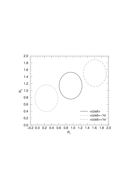
Figure 2: The 1-$\sigma$ allowed regions of $R_{1},R_{2}$ parameters. Three contours are corresponding to $\cos\delta=0.36$ (solid line), $\cos\delta=-0.47$ (dotted line) and $\cos\delta=1.19$ (dashed line), respectively.

Using this result, we can discuss about constraints on the new physics contributions to these processes on the $R_{1}$-$R_{2}$ plane for a given value of $\cos\delta$.

4 Predictions on $R_{1},R_{2}$ in the MSSM and the THDM

Here, we find predictions on $R_{1},R_{2}$ in the MSSM and the THDM. The previous studies on those processes in both models can be found in [18, 19, 20, 21] for $B^{0}\mbox{-}\overline{B^{0}},K^{0}\mbox{-}\overline{K^{0}}$ mixings, and [16, 22, 23] for $K^{+}\rightarrow\pi^{+}\nu\overline{\nu}$ process.

In the MSSM based on $N=1$ supergravity [5], there are several extra particles. Then, interactions among them could be new sources of FCNC processes. It is known that chargino –$t$-squark exchange and charged Higgs–$t$-quark exchange processes give the leading contributions to FCNC processes for $B$ and $K$ meson systems. For the chargino contribution, effects from squarks in the first two generations are canceled each other because degeneracy among their masses holds in good approximation. The interactions among the charged Higgs boson and the up-type quarks are the same with those of the type II-THDM [6]. The charged Higgs boson interacts with the up-type quarks through the Yukawa interactions which are proportional to the corresponding quark masses. As a result, the charged Higgs contributions to the FCNC processes are dominated by its interaction with the top-quark.

The magnitudes of both the chargino and the charged Higgs contributions are proportional to $1/\tan\beta$, where $\tan\beta$ is the ratio of the vacuum expectation values of two Higgs fields. The effective Lagrangians for both contributions are described by $V-A$ and $S+P$ operators. The latter can be negligible for small $\tan\beta$. Furthermore, contributions from other sources in the MSSM do not give sizable effects to the FCNC processes for $\tan\beta\,{\mathop{<}\limits_{\sim}}\,10$ [16, 20]. Hence we examine both models in the region $\tan\beta\,{\mathop{<}\limits_{\sim}}\,10$.

The expressions for $R_{1}$ in the MSSM and the THDM can be found in [19]. The MSSM contribution to the decay process $K^{+}\rightarrow\pi^{+}\nu\overline{\nu}$ is expressed by using $D^{\rm new}$ as follows

$$D^{\rm new}(i)=\sum_{m,n,k,\alpha,\beta}D_{C}(i,m,n;\ell,k;\alpha,\beta)+D_{H}(i,\ell),$$ (4.1)

where $D_{C}(i,m,n;\ell,k;\alpha,\beta)$ and $D_{H}(i,\ell)$ represent the chargino and the charged Higgs boson contributions, respectively. Their explicit forms are given in [15]. For $D_{C}$, by using the unitarity of the CKM matrix and the degeneracy of the squark masses between the first two generations, we obtain

$$V_{i2}^{*}V_{i1}D_{C}(i,m,n;\ell,k;\alpha,\beta)=V_{32}^{*}V_{31}\biggl{\{}D_{C}(3,m,n;\ell,k;\alpha,\beta)-D_{C}(1,m,n;\ell,k;\alpha,\beta)\biggr{\}},$$ (4.2)

and the chargino contribution $A^{\rm new}\equiv A_{C}$ is given by

$$A_{C}\equiv\sum_{m,n,k,\alpha,\beta}\biggl{\{}D_{C}(3,m,n;\ell,k;\alpha,\beta)-D_{C}(1,m,n;\ell,k;\alpha,\beta)\biggr{\}}.$$ (4.3)

Figure 3: The MSSM (left) and THDM (right) contributions to $R_{1}$ and $R_{2}$ parameters for $\tan\beta=2$. The 1-$\sigma$ allowed region of $R_{1}$ and $R_{2}$ parameters for $\cos\delta=0.36$ is also shown.

For $D_{H}$, due to the smallness of the Yukawa couplings for light quarks, we can write the charged Higgs contribution as

$$A_{H}\equiv D_{H}(3,\ell).$$ (4.4)

From (4.3) and (4.4), $R_{2}$ in the MSSM is defined as

$$R_{2}\equiv\frac{D_{W}(3)+A_{C}+A_{H}}{D_{W}(3)}.$$ (4.5)

On the other hand, the THDM contribution to $R_{2}$ is given by setting $D_{C}=0$ in (4.5):

$$R_{2}\equiv\frac{D_{W}(3)+A_{H}}{D_{W}(3)}.$$ (4.6)

Let us proceed numerical study. In order to reduce the number of input parameters in the MSSM, we express the soft SUSY breaking scalar masses in the sfermion sector by a common mass parameter $m_{0}$. Also taking the scalar trilinear coupling $A_{f}$ for sfermion $\tilde{f}$ as $A_{f}=m_{0}$, the MSSM contributions can be evaluated by using four parameters, $m_{0},\tan\beta$, the higgsino mass term $\mu$ and the SU(2) gaugino mass term $m_{2}$. In our study, these parameters are taken to be real. In Fig. 3, we show the MSSM and THDM contributions to $R_{1},R_{2}$ parameters with the constraints on these parameters for $\cos\delta=0.36$. The numerical study was performed in the range of $100~{}{\rm GeV}<m_{0}<1~{}{\rm TeV},|\mu|<200~{}{\rm GeV}$ and $m_{2}=200~{}{\rm GeV}$ for $\tan\beta=2$. We fixed the charged Higgs boson mass at $m_{H}=200~{}{\rm GeV}$ in the MSSM prediction. This is the reason why the MSSM contributions do not converge to $R_{1}=1$ in the figure. We take into account the recent estimation of lower mass limits for lighter $t$-squark and lighter chargino [24]: $80~{}{\rm GeV}\leq m_{\tilde{t}1}$ and $91~{}{\rm GeV}\leq m_{\tilde{\omega}1}$. The MSSM contribution to $R_{1}$ interferes with that of the SM constructively [19, 20, 25]. On the other hand, the contribution to $R_{2}$ interferes with that of the SM both constructively and destructively. Contrary to the case of the MSSM, the THDM contribution constructively interferes with the SM contribution for both $R_{1}$ and $R_{2}$. The Yukawa interaction between the top-quark and the charged Higgs boson is proportional to $1/\tan^{2}\beta$. Thus constraints on the THDM contribution to these quantities are weakened together with the increase of $\tan\beta$.

5 Summary

We have studied impacts on searching for signatures of new physics beyond the SM from some FCNC processes – $B^{0}\mbox{-}\overline{B^{0}},K^{0}\mbox{-}\overline{K^{0}}$ mixings and the rare decay $K^{+}\rightarrow\pi^{+}\nu\overline{\nu}$. For a certain class of models of new physics, two parameters $R_{1}$ and $R_{2}$ were introduced to estimate the new physics contributions to $B^{0}\mbox{-}\overline{B^{0}},K^{0}\mbox{-}\overline{K^{0}}$ mixings and $K^{+}\rightarrow\pi^{+}\nu\overline{\nu}$ decay, respectively. Then constraints on the new physics contributions are obtained from experimental data by using these parameters and $\cos\delta$.

Taking account of both experimental and theoretical uncertainties for the $B^{0}\mbox{-}\overline{B^{0}}$ and $K^{0}\mbox{-}\overline{K^{0}}$ mixings, we found current constraint on $R_{1}$ as $0.18\,{\mathop{<}\limits_{\sim}}\,R_{1}\,{\mathop{<}\limits_{\sim}}\,1.68$. With the assumption that the future data of Br($K^{+}\rightarrow\pi^{+}\nu\overline{\nu}$) will be close to the SM prediction, constraints on $\cos\delta,R_{1}$ and $R_{2}$ were found. The results were applied to the MSSM and the THDM contributions to those processes. Although there are parameter space which give roughly 50% enhancement of $R_{1}$, contributions to $R_{2}$ are less than $\pm 10\%$. So quite precise experimental measurement of $K^{+}\rightarrow\pi^{+}\nu\overline{\nu}$ is required to study constraints on the parameter space of these models.

References

- [1] Particle Data Group, R.M. Barnett et al., Phys. Rev. D54 (1996) 1.
- [2] G. Buchalla, A.J. Buras and M.E. Lautenbacher, Rev. Mod. Phys. 68 (1996) 1125.
-
[3]
J. Ellis and J.S. Hagelin,
Nucl. Phys. B217 (1983) 189;
D. Rein and L.M. Sehgal, Phys. Rev. D39 (1989) 3325;
J.S. Hagelin and L.S. Littenberg, Prog. Part. Nucl. Phys. 23 (1989) 1;
C.Q. Gang, I.J. Hsu and Y.C. Lin, Phys. Lett. B355 (1995) 569;
S. Fajfer, Nuov. Cim. A110 (1997) 397. - [4] E787 collaboration, Phys. Rev. Lett. 79 (1997) 2204.
-
[5]
For reviews, see,
H.P. Nilles, Phys. Rep. 110 (1984) 1,
H.E. Haber and G.L. Kane, Phys. Rep. 117 (1985) 75. - [6] See, e.g., J.F. Gunion, H.E. Haber, G.L. Kane and S. Dawson, The Higgs Hunter’s Guide, Addison-Wesley, (1990) and references therein.
- [7] T. Inami and C.S. Lim, Prog. Theor. Phys. 65 (1981) 297; (E) 1772.
- [8] G. Buchalla and A.J. Buras, Nucl. Phys. B400 (1993) 225.
- [9] G. Buchalla and A.J. Buras, Phys. Rev. D54 (1996) 6782.
- [10] W.J. Marciano and Z. Parsa, Phys. Rev. D53 (1996) R1.
-
[11]
A.J. Buras and R. Fleischer, hep-ph/9704376;
A.J. Buras, hep-ph/9711217. - [12] A.J. Buras, M. Jamin and P.H. Weisz, Nucl. Phys. B347 (1990) 491.
- [13] A. Abada, et al., Nucl. Phys. B376 (1992) 172. A. Abada, LPTHE Orsay-94/57.
-
[14]
S. Herrlich and U. Nierste, Nucl. Phys. B419 (1994) 292;
S. Herrlich and U. Nierste, Phys. Rev. D52 (1995) 6505, Nucl. Phys. B476 (1996) 27. - [15] G.C. Cho, to appear in Euro. Phys. Journal. C.
- [16] A.J. Buras, A. Romanio and L. Silvestrini, hep-ph/9712398.
-
[17]
CDF Collaboration, J. Lys, talk at ICHEP96,
in Proc. of ICHEP96,
(ed) Z. Ajduk and A.K. Wroblewski, World Scentific, (1997);
D0 Collaboration, S. Protopopescu, talk at ICHEP96, in the proceedings.
P. Tipton, talk at ICHEP96, in the proceedings. -
[18]
T. Kurimoto, Phys. Rev. D39 (1989) 3447;
S. Bertolini, F. Borzumati, A. Masiero and G. Ridolfi, Nucl. Phys. B353 (1991) 591;
G. Couture and H. König, Z. Phys. C69 (1996) 499. - [19] G.C. Branco, G.C. Cho, Y. Kizukuri and N. Oshimo, Phys. Lett. B337 (1994) 316; Nucl. Phys. B449 (1995) 483.
- [20] T. Goto, T. Nihei and Y. Okada, Phys. Rev. D53 (1996) 5233; (E) D54 (1996) 5904.
- [21] L.F. Abott, P. Sikivie and M.B. Wise, Phys. Rev. D21 (1980) 1393.
-
[22]
S. Bertolini and A. Masiero, Phys. Lett. B174 (1986) 343;
B. Mukhopadhyaya and A. Raychaudhuri, Phys. Lett. B189 (1987) 203;
I.I. Bigi and F. Gabbiani, Nucl. Phys. B367 (1991) 3;
G. Couture and H. König, Z. Phys. C69 (1995) 167;
Y. Nir and M.P. Worah, hep-ph/9711215. - [23] A.J. Buras, P. Krawczyk, M.E. Lautenbacher and C. Salazar, Nucl. Phys. B337 (1990) 284.
- [24] P. Janot, talk given at International Europhysics Conference on High Energy Physics, Jerusalem 1997.
- [25] T. Kurimoto, Mod. Phys. Lett. A10 (1995) 1577.