On the enhancement of the QCD running coupling in the noncontractible space and anomalous TeVatron and HERA data

We show that the existence of the fundamental ultraviolet cut-off (minimal scale) fixed by weak interactions enhances the QCD running coupling evaluated at one quantum loop level, starting at the scale in the vicinity of the cut-off. The enhancement of the QCD running coupling could completely explain the observed anomalous TeVatron and HERA data. The QCD in the noncontractible space is not an asymptotically free gauge theory.

PACS:
11.10.Hi Renormalization group evolution and parameters
12.38.-t Quantum chromodynamics
12.60.-i Models beyond the standard model

1 Introduction

We are entering into the era of the very important measurements in particle physics as well as in cosmology and astrophysics. One expects the assurance of the results that indicate the existence of massive neutrinos and lepton flavour mixing coming from the solar and atmospheric neutrino data, LSND experiment and from various astrophysical and cosmological data relevant for measuring cosmic mass density and structure formation in the Universe. The anomalous events in particle physics observed at high energy hadron-hadron collisions at TeVatron and lepton-hadron collisions at HERA are especially intriguing.

All these results strongly support the necessity to modify, enlarge or improve the Standard Model(SM) of particle physics. It has been recently proposed [1] a mechanism for the gauge symmetry breaking without the introduction of the Higgs scalar. The ultraviolet singularity and the SU(2) global anomaly problems appear as milestone points that could lead to the improvement of the SM. Namely, the embedding of the SU(2) gauge symmetry into the SU(3) symmetry gives the natural and unique solution of the nonperturbative consistency with respect to the SU(2) anomaly, while the hypothesis of the noncontractible space triggers the violation of gauge, discrete and conformal symmetries [1].

The qualitative analysis of bootstrap equations in the nonsingular theory can give the insight into the understanding of the problem of a number of fermion families, mass gaps between the families, the smallness of neutrino masses, etc. The lepton number is spontaneously broken and neutrinos appear as Majorana particles. The neutrino masses are cosmologically acceptable and confirmed by Super-Kamiokande [2], the heaviest light neutrino could play the role of the hot dark matter particle [1, 3] and one of heavy neutrinos could be a candidate for the cold dark matter [4]. We are in a position to solve the problem of the baryogenesis through leptogenesis because of the broken lepton number. A calculation of the $\eta$- parameter of the cosmological nucleosynthesis [3] could cause a severe test of the theory.

Introducing into the theory the fundamental scale defined by weak interactions, as the only fundamental interaction that can provide nonvanishing dimensionfull quantity-the mass of the weak gauge boson, one has to check the relevance of this scale in the gravity and cosmology. We claim [5] that the weak scale is also a natural fundamental scale in the Einstein-Cartan nonsingular cosmology where torsion plays a crucial role in preventing the appearance of the cosmological singularity. However, the greatest challenge of the Einstein-Cartan cosmology is the possibility to solve the problem of the mass density of the Universe and the cosmological constant problem (without fine-tuning) at the space-like infinity ($T_{\gamma}=0K$), that means at the time when the Universe is very similar to its present evolutionary stage ($T_{\gamma}=2.73K$) [5]. In addition, the existence of the spinning dark matter particles (light and heavy neutrinos) and the global vorticity of the Universe are required. [4, 5, 6] The EC cosmology can also solve the problem of the primordial mass density fluctuation [7].

It has been also shown that the effect of the fundamental length in quantum mechanics [8] is the spectrum-line broadening that is proportional to the square of the fundamental length $\Delta E\propto(\frac{d}{R})^{2}$. Lee’s discrete quantum mechanics (quantum mechanics on the lattice) gives different observable phenomena with different bounds and estimates [9].

This paper is devoted to the study of the QCD running coupling in the noncontractible space at one quantum loop and its comparison with the SM calculations. In the next section we present the perturbative calculation supplied with all the necessary details in the Appendix. In the concluding section we outline numerical results and discuss their relevance with respect to the recently observed anomalous events at TeVatron and HERA.

2 Perturbative calculus of the QCD running coupling

The UV cut-off is fixed in a gauge and Lorentz invariant manner applying the Wick’s theorem in the trace anomaly [1]. Contrary to other scale fixing procedures, such as in the nonlocal gauge theory through the nonuniversal functionals, the relation for the weak boson mass is similar to that of the Higgs mechanism but now instead of the vacuum expectation value of the scalar field figures the universal cut-off (modulo real number), thus defined by the gauge and Lorentz invariant quantities, namely the weak boson mass and the weak coupling constant [1]: $\Lambda=\frac{2\pi}{\sqrt{6}g}M_{W}=\frac{\hbar}{cd}$.

We can use all formalisms of the local relativistic quantum gauge field theory for the broken (QFD) and the unbroken (QCD) phase of the theory. The above relation should be preserved to all orders in perturbation theory and it should be considered as a definition of the universal fundamental scale . Operator gauge- and Heisenberg-algebras are intact by this consideration, no new operators emerge and one can use all the benefits of the BRST symmetry, such as the generalized Ward-Takahashi and Slavnov-Taylor identities for the Green’s functions and the renormalizability of the non-Abelian gauge theory [1].

The calculations will be performed in the ’t Hooft-Feynman gauge with constant nonvanishing quark masses. We choose the definition of the running coupling originating from the light quark-gluon vertex [10].

The momentum subtraction renormalization scheme [11] appears as the naturally suitable scheme for the UV finite theory and we shall apply it to the QCD, with and without the fundamental scale.

The following conventions are adopted for the renormalization constants [12] :

$$\alpha=Z^{-1}_{\alpha}\alpha_{0},\ Z_{\alpha}=(\frac{Z_{1F}}{Z_{2F}})^{2}Z^{-1}_{3YM},\hskip 65.44133pt$$

$$G^{\mu}_{a0}(x)=Z^{1/2}_{3YM}G^{\mu}_{a}(x),\ q^{A}_{\alpha 0}(x)=Z^{1/2}_{2F}q^{A}_{\alpha}(x),\hskip 28.45274pt$$ (1)

$$g_{0F}=Z_{1F}Z^{-1/2}_{3YM}Z^{-1}_{2F}g_{F},\ \beta(\alpha)=Z_{\alpha}\mu\frac{dZ^{-1}_{\alpha}}{d\mu}=\alpha^{-1}\mu\frac{d\alpha}{d\mu}.$$

The off-mass-shell renormalization conditions define the following physical (renormalized) Green’s functions:

$$S^{R}(\not p)_{p^{2}=-\mu^{2}}=S_{F}(\not p)_{p^{2}=-\mu^{2}},\hskip 45.5244pt$$

$$\ \Gamma^{R}_{\nu}(p,q)_{p^{2}=q^{2}=-\mu^{2}}=\gamma_{\nu},\hskip 71.13188pt$$ (2)

$$asymmetric\ condition:\ p^{2}=q^{2}\neq(p+q)^{2}.\hskip 28.45274pt$$

To insure the SU(3) gauge invariance we impose the on-mass-shell renormalization condition for the polarization operator of the gluon field [13]:

$$\Pi^{on}_{R}(p)_{p^{2}=0}=0.$$ (3)

The above conditions define the infinite and finite parts of the renormalization constants in the SM and the finite renormalization constants in the UV-finite theory.

We have now to relate renormalization constants of the polarization operator in two distinct (off- and on-mass-shell) renormalization schemes:

$$\Pi^{on}_{R}(p,m_{i},\Lambda)=Z^{on}_{3YM}(p,m_{i},\Lambda)\Pi_{0}(p,m_{i},,\Lambda),\hskip 85.35826pt$$

$$\Pi^{off}_{R}(p,m_{i},\mu,\Lambda)=Z^{off}_{3YM}(\mu,m_{i},\Lambda)\Pi_{0}(p,m_{i},\Lambda),\hskip 85.35826pt$$ (4)

$$\ \Lambda=fundamental\ UV\ cut-off,\mu=scale\ parameter.\hskip 71.13188pt$$

The evaluation of the $\beta$-function requires the knowledge of the derivative of the renormalization constant with respect to the scale variable:

$$\frac{\partial Z^{off}_{3YM}(\mu,m_{i},\Lambda)}{\partial ln\mu}=\frac{\partial\Pi_{R}^{off}(p,m_{i},\mu,\Lambda)}{\partial ln\mu}.$$ (5)

Because of the universality of the $\beta$-function to the one-loop order and Eq.(4), the following relation must be fulfilled:

$$\frac{\partial\Pi^{off}_{R}(p,m_{i},\mu,\Lambda)}{\partial ln\mu}=\frac{\partial\Pi^{on}_{R}(\mu^{2}=-\frac{1}{p^{2}},m_{i},\Lambda)}{\partial ln\mu}.$$ (6)

By the choice for the scale variable $\mu^{2}=-\frac{1}{p^{2}}$ in the on-mass-shell scheme, it is possible to compare the physical quantities at various spacelike points up to the spacelike infinity. It is in accordance with the on-mass-shell renormalization condition at $p^{2}=0$ for the polarization operator. Thus, we can conclude that:

$$\frac{\partial Z^{off}_{3YM}(\mu,m_{i},\Lambda)}{\partial ln\mu}=-\frac{\partial\Pi^{on}_{R}(\mu^{2}=-p^{2},m_{i},\Lambda)}{\partial ln\mu}.$$ (7)

One can immediately evaluate (see Ref.[12] or any textbook on the QCD) the necessary renormalization constants from the quark-gluon vertex, quark and gluon self-energy diagrams in the   ’t Hooft-Feynman gauge in terms of one-, two- and three-point Green’s functions(see Appendix):

$$Z_{i}=1+\delta Z_{i},\hskip 156.49014pt$$

$$\delta Z_{1F}=\frac{\alpha_{s}}{4\pi}[\frac{1}{6}(2B_{0}(4p^{2};0,m_{q})-4C_{2}^{a}(p,2p;m_{q},m_{q})+2p^{2}C_{0}(p,2p;m_{q},m_{q})$$

$$+2p^{2}C_{1}(p,2p;m_{q},m_{q}))-\frac{3}{2}(2B_{0}(4p^{2};0,m_{q})+p^{2}C_{1}(p,-p;0,m_{q})$$

$$+4C_{2}^{a}(p,-p;0,m_{q})-p^{2}C_{0}(p,-p;0,m_{q}))]_{p^{2}=-\mu^{2}},\hskip 59.75078pt$$

$$\delta Z_{2F}=-\frac{\alpha_{s}}{4\pi}\frac{8}{3}[B_{0}(-\mu^{2};0,m_{q})+B_{1}(-\mu^{2};0,m_{q})],\hskip 56.9055pt$$

$$\delta Z_{3YM}=\frac{\alpha_{s}}{4\pi}[-\frac{1}{3}\sum_{f}(2B_{0}(-\mu^{2};m_{f},m_{f})-\frac{4m_{f}^{2}}{\mu^{2}}(B_{0}(-\mu^{2};m_{f},m_{f})$$

$$-B_{0}(0;m_{f},m_{f}))+5B_{0}(-\mu^{2};0,0)]+\chi(m_{i},\Lambda).$$ (8)

From the standard definition of the $\beta$ function [12] we can easily find the relation for the QCD running coupling to one quantum loop:

$$\beta(\alpha_{s})\simeq\alpha_{s}\beta_{1}(\mu);\ -\frac{1}{\alpha_{s}(\mu)}+\frac{1}{\alpha_{s}(\mu_{0})}=\int^{\mu}_{\mu_{0}}\frac{\beta_{1}(\kappa)}{\kappa}d\kappa,\hskip 28.45274pt$$

$$\beta_{1}(\mu)\equiv\mu\frac{d\Phi(\mu)}{d\mu},\hskip 85.35826pt$$

$$\alpha_{s}(\mu)=\frac{\alpha_{s}(\mu_{0})}{1+\alpha_{s}(\mu_{0})(\Phi(\mu_{0})-\Phi(\mu))},\hskip 56.9055pt$$ (9)

$$\Phi(\mu)=\alpha_{s}^{-1}(-2\delta Z_{1F}+2\delta Z_{2F}+\delta Z_{3YM}).\hskip 36.98857pt$$

Eqs. (8) and (9) give immediately the standard relation for the QCD running coupling in the SM with massless quarks:

$$\Phi(\mu_{0})-\Phi(\mu)=\frac{11-\frac{2}{3}n_{f}}{2\pi}ln\frac{\mu}{\mu_{0}}.$$

To derive the above formula we used the following relations:

$$\frac{\partial B^{\infty}_{0}(-\mu^{2};0,0)}{\partial ln\mu}=-2,\ \frac{\partial[\mu^{2}C^{\infty}_{0}(-\mu^{2};0,0)]}{\partial ln\mu}=2.$$ (10)

Throughout the paper the superscripts ”$\infty$” or ”$\Lambda$” denote the physical quantities evaluated in the standard way or with the covariant UV-cut-off $\Lambda$.

Before turning to the numerical study of our basic result Eq.(9), we should comment three important points: (1) to preserve the gauge invariance in the case of $\Lambda<\infty$, it is essential to fulfil condition of Eq.(3) by which ${\cal O}(\Lambda^{2})$ terms are subtracted away, (2) the dependence of the observables on the covariant spacelike cut-off $\Lambda$ is completely hidden in the integration region of the scalar integrals; one should not confuse this cut-off with some regularization cut-off because for the theory with $\Lambda<\infty$ there is a unique integration and a nontrivial analytical continuation procedure for timelike external momenta (for details see Appendix), (3) the scaling variable $\mu$ can acquire arbitrary value (it is not limited by the cut-off) because even for $\Lambda<\infty$ the theory is a local gauge theory.

3 Results and discussion

We can now illustrate the effect of the fundamental UV cut-off on the QCD running coupling, applying Eqs. (8) and (9) to the Green’s functions with and without the UV cut-off. To make a comparison we choose the following set of the initial conditions and quark massess[14, 15] ($\alpha_{s}^{\infty}\equiv\alpha_{s}(SM)$) :

$$Input\ parameters\ for\ Eq.(9):\hskip 187.78818pt$$

$$\Lambda=326\ GeV,\ \alpha_{s}(\mu_{0})=0.12,\ \mu_{0}=M_{Z}=91.19\ GeV,\ n_{f}=6,\hskip 56.9055pt$$

$$m_{u}=6\ MeV,\ m_{d}=9\ MeV,\ m_{s}=160\ MeV,\hskip 113.81102pt$$

$$m_{c}=1.5\ GeV,\ m_{b}=4.5\ GeV,\ m_{t}=175\ GeV\hskip 105.27519pt$$

In Figure 1 one can notice the enhancement of the running coupling $\alpha^{\Lambda}_{s}$ in comparison with $\alpha^{\infty}_{s}$, starting at the scale in the vicinity of the UV cut-off. We have displayed $\alpha_{s}^{2}$ values because the differential cross sections of various hadron-hadron collisions are proportional to $\alpha_{s}^{2}$. The enhancement of the inclusive jet cross section at high $E_{T}$ and the excess in the production of W(Z) plus one jet are observed at TeVatron [16, 17].

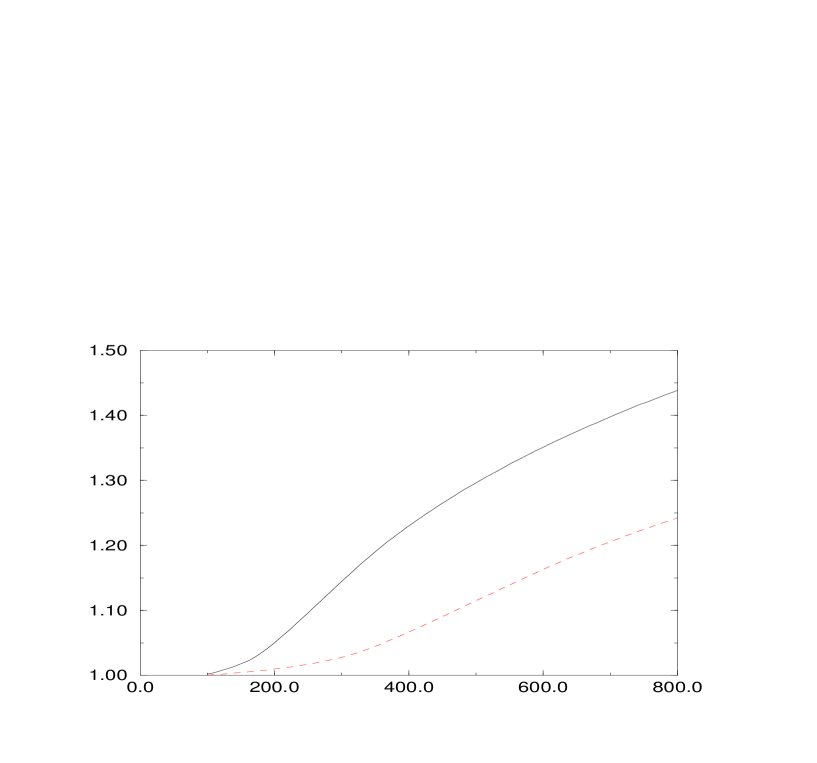
Figure 1: Solid [dashed] line denotes $(\alpha^{\Lambda}_{s}/\alpha^{\infty}_{s})^{2}$ vs. $\mu(GeV)$ for $\Lambda$= 326 [600] GeV.

In order to show the sensitivity of the results on the magnitude of the fundamental UV cut-off, one can observe in Figure 1 the smaller effect for larger cut-off $\Lambda$.

The effects of running masses or two loop corrections cannot alter our conclusion on the persistent enhancement of $\alpha_{s}^{\Lambda}(\mu)$ for $\mu\geq 200GeV$.

The leading order calculation of the Altarelli-Parisi equations [18, 19] shows that there is a very small enhancement of parton distribution functions for small x and very small suppression for large x at $Q\geq 200GeV$ (see Figs. 2 and 3).

Figure 2: Solid line denotes $xF_{1}^{\Lambda}(x,Q^{2})$ vs. x for Q=300 GeV and $\Lambda$=326 GeV.

Figure 3: Solid line denotes $(xF_{1}^{\Lambda}-xF_{1}^{\infty})/(xF_{1}^{\infty})$ vs. x for Q=300 GeV.

QCD corrections to the electroweak couplings could generate enhancement above the scale $\mu\simeq 200GeV$. This effect is observed at HERA and LEP 2 [20, 21]:

$$|V_{EW+QCD}(q^{2})|^{2}=|V_{EW}(q^{2})|^{2}[1+\frac{\alpha_{s}(q^{2})}{\pi}+{\cal O}(\alpha^{2}_{s}(q^{2}))],$$

$$enhancement\ factor=\ [1+\frac{\alpha_{s}^{\Lambda}(q^{2})}{\pi}]/[1+\frac{\alpha_{s}^{\infty}(q^{2})}{\pi}].$$

To conclude, one can say that the effect of the noncontractible space in QCD is the nonresonant and universal enhancement of various cross sections in $p\bar{p}$ and $ep$ collisions (this conclusion is verified in the region where one can apply the perturbative calculus), starting at the scale in the vicinity of the UV cut-off. The characteristics of the anomalous TeVatron and HERA data are in accordance with this claim [16, 20]. Above the scale of $\mu\simeq 500\ GeV$ the QCD coupling $\alpha^{\Lambda}_{s}$ is frozen at some nonvanishing value, for example $\lim_{\mu\rightarrow\infty}\alpha^{\Lambda}_{s}(\mu)=0.11$ with parameters of Figure 1. The enhancement at the scale relevant at LHC is: $(\frac{\alpha^{\Lambda}_{s}}{\alpha^{\infty}_{s}})^{2}(\mu=few\ TeV)\simeq 2-4$. Evidently, the QCD in the noncontractible space is not an asymptotically free gauge field theory [22].

Appendix

We use the following definitions and settings of the Green’s functions with the UV cut-off ($\Lambda$ superscript) and the SM ones($\infty$ superscript)

$$A(m)=-\frac{1}{\imath\pi^{2}}\int d^{4}q\frac{1}{q^{2}-m^{2}+\imath\varepsilon},$$

$$B_{0}(p^{2};m_{1},m_{2})=\frac{1}{\imath\pi^{2}}\int d^{4}q\frac{1}{(q^{2}-m_{1}^{2}+\imath\varepsilon)((q+p)^{2}-m_{2}^{2}+\imath\varepsilon)},$$

$$p_{\mu}B_{1}(p^{2};m_{1},m_{2})=\frac{1}{\imath\pi^{2}}\int d^{4}q\frac{q_{\mu}}{(q^{2}-m_{1}^{2}+\imath\varepsilon)((q+p)^{2}-m_{2}^{2}+\imath\varepsilon)},$$

$$C_{0}(p_{1},p_{2};m_{1},m_{2})=\frac{1}{\imath\pi^{2}}\int d^{4}q\frac{1}{(q^{2}+\imath\varepsilon)((q+p_{1})^{2}-m_{1}^{2}+\imath\varepsilon)((q+p_{2})^{2}-m_{2}^{2}+\imath\varepsilon)},$$

$$p_{1\mu}C_{1}(p_{1},p_{2};m_{1},m_{2})=\frac{1}{\imath\pi^{2}}\int d^{4}q\frac{q_{\mu}}{(q^{2}+\imath\varepsilon)((q+p_{1})^{2}-m_{1}^{2}+\imath\varepsilon)((q+p_{2})^{2}-m_{2}^{2}+\imath\varepsilon)},$$

$$g_{\mu\nu}C^{a}_{2}(p_{1},p_{2};m_{1},m_{2})+p_{1\mu}p_{1\nu}C^{b}_{2}(p_{1},p_{2};m_{1},m_{2})=$$

$$=\frac{1}{\imath\pi^{2}}\int d^{4}q\frac{q_{\mu}q_{\nu}}{(q^{2}+\imath\varepsilon)((q+p_{1})^{2}-m_{1}^{2}+\imath\varepsilon)((q+p_{2})^{2}-m_{2}^{2}+\imath\varepsilon)},$$

$$2p^{2}B_{1}(p^{2};m_{1},m_{2})=A(m_{2})-A(m_{1})+(m_{2}^{2}-m_{1}^{2}-p^{2})B_{0}(p^{2};m_{1},m_{2}),$$

$$2p_{1}^{2}C_{1}(p_{1},p_{2};m_{1},m_{2})=B_{0}(p_{2}^{2};0,m_{2})-B_{0}((p_{2}-p_{1})^{2};m_{1},m_{2})$$

$$+(m_{1}^{2}-p_{1}^{2})C_{0}(p_{1},p_{2};m_{1},m_{2}),\hskip 45.5244pt$$

$$C_{2}^{a}=\frac{1}{3}(\Delta_{1}-\Delta_{2}),\ C_{2}^{b}=\frac{1}{3p_{1}^{2}}(4\Delta_{2}-\Delta_{1}),\hskip 119.50157pt$$

$$\Delta_{1}=B_{0}((p_{2}-p_{1})^{2};m_{1},m_{2}),\hskip 119.50157pt$$

$$\Delta_{2}=\frac{1}{2}[B_{0}((p_{2}-p_{1})^{2};m_{1},m_{2})+\kappa B_{1}(p_{2}^{2};0,m_{2})+(1-\kappa)B_{1}((p_{2}-p_{1})^{2};m_{1},m_{2})$$

$$+(m_{1}^{2}-p_{1}^{2})C_{1}(p_{1},p_{2};m_{1},m_{2})],\hskip 219.08621pt$$

$$p_{2\mu}=\kappa p_{1\mu},\hskip 170.71652pt$$

$$A^{\Lambda}(m)=\Lambda^{2}-m^{2}ln(\frac{\Lambda^{2}+m^{2}}{m^{2}}),\hskip 85.35826pt$$

$$B_{0}^{\Lambda}(p^{2};m_{1},m_{2})=\frac{1}{2}[\tilde{B}_{0}^{\Lambda}(p^{2};m_{1},m_{2})+\tilde{B}_{0}^{\Lambda}(p^{2};m_{2},m_{1})],$$

$$Re\tilde{B}_{0}^{\Lambda}(p^{2};m_{1},m_{2})=(\int_{0}^{\Lambda^{2}}dyK(p^{2},y)+\theta(p^{2}-m_{2}^{2})\int_{-(\sqrt{p^{2}}-m_{2})^{2}}^{0}dy\Delta K(p^{2},y))\frac{1}{y+m_{1}^{2}},$$

$$K(p^{2},y)=\frac{2y}{-p^{2}+y+m_{2}^{2}+\sqrt{(-p^{2}+y+m_{2}^{2})^{2}+4p^{2}y}},\hskip 113.81102pt$$

$$\Delta K(p^{2},y)=\frac{\sqrt{(-p^{2}+y+m_{2}^{2})^{2}+4p^{2}y}}{p^{2}}.\hskip 170.71652pt$$

The integration in the second term [23] is performed from the branch point of the square root $\sqrt{(-p^{2}+y+m_{2}^{2})^{2}+4p^{2}y}\equiv\imath Z$ and the additional kernel is derived as the difference: $\Delta K(p^{2},y)=K(p^{2},y)-K^{*}(p^{2},y)=\frac{2y}{-p^{2}+y+m_{2}^{2}+\imath Z}-\frac{2y}{-p^{2}+y+m_{2}^{2}-\imath Z}$.

The integration over singularities is supposed to be the principal value integration.

$$C_{0}^{\Lambda}(p_{1}^{2},(p_{2}-p_{1})^{2},p_{2}^{2};0,m_{1}^{2},m_{2}^{2})=\frac{1}{3}[\tilde{C}_{0}^{\Lambda}(p_{1}^{2},(p_{2}-p_{1})^{2},p_{2}^{2};0,m_{1}^{2},m_{2}^{2})$$

$$+\tilde{C}_{0}^{\Lambda}((p_{2}-p_{1})^{2},p_{2}^{2},p_{1}^{2};m_{1}^{2},m_{2}^{2},0)+\tilde{C}_{0}^{\Lambda}(p_{2}^{2},p_{1}^{2},(p_{2}-p_{1})^{2};m_{2}^{2},0,m_{1}^{2})],$$

$$Re\tilde{C}_{0}^{[\Lambda;\infty]}(123)=-\frac{4}{\pi}\int^{[\Lambda;\infty]}_{0}dqq\hskip 56.9055pt$$

$$\times\int^{+1}_{-1}dx\sqrt{1-x^{2}}\frac{1}{q^{2}+p_{1}^{2}+m_{1}^{2}+2qp_{1}x}\frac{1}{q^{2}+p_{2}^{2}+m_{2}^{2}+2qp_{2}x},$$

$$p_{1}^{\mu}=(0,0,0,p_{1}),\ p_{2}^{\mu}=(0,0,0,p_{2}),\hskip 113.81102pt$$

$$similarly\ for\ \tilde{C}_{0}^{\Lambda}(231)\ and\ \tilde{C}_{0}^{\Lambda}(312).$$

Symmetrization over external momenta is included in order to restore the momentum-exchange symmetry when $\Lambda<\infty$ (broken scale symmetry).

The integrals for high momenta up to infinity should be performed after the inverse mapping of the integration variable. For massive quarks and off-shell external momenta Green’s functions are infrared convergent [24].

In the case of the two-point Green’s function $B_{0}^{\Lambda}$ we need the explicit form of the additional term for the integration in the timelike region because the integration in the spacelike region in the limes $\Lambda\rightarrow\infty$ is divergent. However, the three-point scalar Green’s functions are UV-convergent and we do not need to know the explicit form of the additional terms because they do not depend on the UV cut-off and we can use the analytical continuation of the standard Green’s functions written in terms of the dilogarithms[25]:

$$ReC_{0}^{\Lambda}(p_{i},m_{j})=\int_{0}^{\Lambda^{2}}dq^{2}\Phi(q^{2},p_{i},m_{j})+\int_{TD}dq^{2}\Xi(q^{2},p_{i},m_{j}),\hskip 28.45274pt$$

$$ReC_{0}^{\Lambda}(p_{i},m_{j})=ReC_{0}^{\infty}(p_{i},m_{j})-\int^{\infty}_{\Lambda^{2}}dq^{2}\Phi(q^{2},p_{i},m_{j}),\hskip 56.9055pt$$

$$\Phi\equiv function\ derived\ by\ the\ angular\ integration\ after\ Wick^{\prime}s\ rotation,$$

$$C_{0}^{\infty}\equiv standard\ ^{\prime}t\ Hooft-Veltman\ scalar\ function,\hskip 56.9055pt$$

$$TD\equiv timelike\ domain\ of\ integration.\hskip 113.81102pt$$

References

• [1] D. Palle, Nuovo Cimento A 109, 1535 (1996).
• [2] T. Fukuda et al, Phys. Rev. Lett. 81, 1562 (1998).
• [3] E. W. Kolb and M. S. Turner, The Early Universe (Addison-Wesley, Redwood City, 1990).
• [4] D.Palle, Nuovo Cimento B 115, 445 (2000).
• [5] D. Palle, Nuovo Cimento B 111, 671 (1996).
• [6] L.-X. Li, Gen. Rel. Grav. 30, 497 (1998).
• [7] D. Palle, Nuovo Cimento B 114, 853 (1999).
• [8] D. Palle, Nuovo Cimento B 112, 943 (1997).
• [9] T. D. Lee, Phys. Lett. B 122, 217 (1983); L. Bracci, G. Fiorentinni, G. Mezzorani and P. Quarati, ibid. B 133, 231 (1983).
• [10] A. De RΓΊjula and H. Georgi, Phys. Rev. D 13, 1296 (1976); E. C. Poggio, H. R. Quin and S. Weinberg, ibid. D 13, 1958 (1976); H. Georgi and H. D. Politzer, ibid. D 14, 1829 (1976).
• [11] W. Celmaster and R. J. Gonsalves, Phys. Rev. D 20, 1420 (1979).
• [12] P. Pascual and R. Tarrach, QCD: Renormalization for the Practitioner (Springer-Verlag, Berlin, 1984).
• [13] K. Aoki et al, Suppl. Progr. Theor. Phys. 73, 1 (1982); M. BΓΆhm, H. Spiesberger and W. Hollik, Fort. der Physik 34, 687, 1986.
• [14] O. Nachtmann and W. Wetzel, Nucl. Phys. B 146, 273 (1978).
• [15] J. Gasser and H. Leutwyler, Phys. Rep. 87, 77 (1982).
• [16] S. Abachi et al, Phys. Rev. Lett. 75, 3226 (1995); F. Abe et al, ibid. 77, 438 (1996); F. Abe et al, ibid. 79, 4760 (1997); F. Abe et al, ibid. 80, 3461 (1998); T. Affolder et al, Phys. Rev. D 61, 091101 (2000); B. Abbott et al, Phys. Lett. B 487, 264 (2000); B. Abbott et al, hep-ex/0008021; B. Abbott et al, hep-ex/0008072.
• [17] E. W. N. Glover, A. D. Martin, R. G. Roberts and W. J. Stirling, Phys. Lett. B 381, 353 (1996).
• [18] V. N. Gribov and L. N. Lipatov, Sov. J. Nucl. Phys. 15, 438; 675 (1972); Yu. L. Dokshitzer, Sov. Phys. JETP 46, 641 (1977); G. Altarelli and G. Parisi, Nucl. Phys. B 126, 298 (1977).
• [19] M. Miyama and S. Kumano, Comp. Phys. Commun. 94, 185 (1996); M. Hirai, S. Kumano and M. Miyama, Comp. Phys. Commun. 108, 38 (1998).
• [20] C. Adloff et al, Zeit. fΓΌr Physik C 74, 191 (1997); J. Breitweg et al, ibid. C 74, 207 (1997); U. Bassler and G. Bernardi, ibid. C 76, 223 (1997); J. Breitweg et al, Eur. Phys. J. C 11, 35 (1999); J. Breitweg et al, Eur. Phys. J. C 16, 253 (2000); J. Breitweg et al, Phys. Lett. B 481, 213 (2000). 108, 38 (1998).
• [21] D. Palle, hep-ph/0010210.
• [22] D. J. Gross and F. Wilczek, Phys. Rev. Lett. 30, 1343 (1973); H. D. Politzer, ibid. 30, 1346 (1973).
• [23] R. Fukuda and T. Kugo, Nucl. Phys. B 117, 250 (1976).
• [24] J. M. Cornwall and G. Tiktopoulos, Phys. Rev. D 13, 3370 (1976); J. M. Cornwall and G. Tiktopoulos, ibid. D 15, 2937 (1977).
• [25] G. ’t Hooft and M. Veltman, Nucl. Phys. B 153, 365 (1979); G. J. van Oldenborgh and J. A. M.Vermaseren, Zeit. fΓΌr Physik C 46, 425 (1990); G. J. van Oldenborgh, Comp. Phys. Commun. 66, 1 (1991).