Nucleon spin content and axial coupling constants in QCD sum rules approach.

Abstract

The review of current experimental situation in the measurements of the first moment $\Gamma_{p,n}$ of spin dependent nucleon structure functions $g_{1;p,n}(x,Q^{2})$ is presented. The results of the calculations of twist-4 corrections to $\Gamma_{p,n}$ are discussed and their accuracy is estimated. The part of the proton spin $\Sigma$ carried by $u,d,s$ quarks is calculated in the framework of the QCD sum rules in the external fields. The operators up to dimension 9 are accounted. An important contribution comes from the operator of dimension 3, which in the limit of massless $u,d,s$ quarks is equal to the derivative of QCD topological susceptibility $\chi^{\prime}(0)$. The comparison with the experimental data on $\Sigma$ gives $\chi^{\prime}(0)=(2.3\pm 0.6)\times 10^{-3}~{}GeV^{2}$. The limits on $\Sigma$ and $\chi^{\prime}(0)$ are found from selfconsistency of the sum rule, $\Sigma\mathrel{\mathchoice{\lower 3.6pt\vbox{\halign{$\mathsurround=0pt\displaystyle\hfil#\hfil$\cr>\crcr\sim\crcr}}}{\lower 3.6pt\vbox{\halign{$\mathsurround=0pt\textstyle\hfil#\hfil$\cr>\crcr\sim\crcr}}}{\lower 3.6pt\vbox{\halign{$\mathsurround=0pt\scriptstyle\hfil#\hfil$\cr>\crcr\sim\crcr}}}{\lower 3.6pt\vbox{\halign{$\mathsurround=0pt\scriptscriptstyle\hfil#\hfil$\cr>\crcr\sim\crcr}}}}0.05,~{}~{}\chi^{\prime}(0)\mathrel{\mathchoice{\lower 3.6pt\vbox{\halign{$\mathsurround=0pt\displaystyle\hfil#\hfil$\cr>\crcr\sim\crcr}}}{\lower 3.6pt\vbox{\halign{$\mathsurround=0pt\textstyle\hfil#\hfil$\cr>\crcr\sim\crcr}}}{\lower 3.6pt\vbox{\halign{$\mathsurround=0pt\scriptstyle\hfil#\hfil$\cr>\crcr\sim\crcr}}}{\lower 3.6pt\vbox{\halign{$\mathsurround=0pt\scriptscriptstyle\hfil#\hfil$\cr>\crcr\sim\crcr}}}}1.6\times 10^{-3}~{}GeV^{2}$. The values of $g_{A}=1.37\pm 0.10$ and $g^{8}_{A}=0.65\pm 0.15$ are also determined from the corresponding sum rules.

I dedicate this lecture to the memory of my friend Volodya Gribov, whom I knew for about half a centure. Now it becomes even more clear how great was his influence on physics: his brilliant ideas, his uncompromising approach to science, his teaching ability. My loss is even more painful: every meeting with Volodya was like a holyday to my soul.

1.  Introduction. Recent experimental data.

In the last years, the problem of nucleon spin content and particularly the question which part of the nucleon spin is carried by quarks, attracts a strong interest. The valuable information comes from the measurements of the spin-dependent nucleon structure functions $g_{1}(x,Q^{2})$ in deep inelastic $e(\mu)N$ scattering (for the recent data see [1,2,3], for a reviews [4,5]). The parts of the nucleon spin carried by $u,d$ and $s$-quarks are determined from the measurements of the first moment of $g_{1}(x,Q^{2})$

$$\Gamma_{p,n}(Q^{2})=\int\limits_{0}^{1}dxg_{1;p,n}(x,Q^{2})$$ (1)

At high $Q^{2}$ with the account of twist-4 contributions $\Gamma_{p,n}(Q^{2})$ have the form

$$\Gamma_{p,n}(Q^{2})=\Gamma^{as}_{p,n}(Q^{2})+\Gamma^{tw4}_{p,n}(Q^{2})$$ (2)

$$\Gamma^{as}_{p,n}(Q^{2})=\frac{1}{12}\Biggl{\{}[1-\bar{\alpha}-3.58\bar{\alpha}^{2}-20.2\bar{\alpha}^{3}-c\bar{\alpha}^{4}][\pm g_{A}+\frac{1}{3}g^{8}_{A}]$$

$$+\frac{4}{3}[1-\frac{1}{3}\bar{\alpha}-0.55\bar{\alpha}^{2}-4.45\bar{\alpha}^{3}]\Sigma\Biggr{\}}-\frac{N_{f}}{18\pi}\alpha_{s}(Q^{2})\Delta g(Q^{2})$$ (3)

$$\Gamma^{tw4}_{p,n}(Q^{2})=\frac{b_{p,n}}{Q^{2}}$$ (4)

In eq.(3) $\bar{\alpha}=\alpha_{s}(Q^{2})/\pi,g_{A}$ is the $\beta$-decay axial coupling constant, $g_{A}=1.260\pm 0.002$ [6]

$$g_{A}=\Delta u-\Delta d~{}~{}~{}~{}g^{8}_{A}=\Delta u+\Delta d-2\Delta s~{}~{}~{}~{}\Sigma=\Delta u+\Delta d+\Delta s.$$ (5)

$\Delta u,\Delta d,\Delta s,\Delta g$ are parts of the nucleon spin projections carried by $u,d,s$ quarks and gluons:

$$\Delta q=\int\limits^{1}_{0}\Biggl{[}q_{+}(x)-q_{-}(x)\Biggr{]}dx$$ (6)

where $q_{+}(x),q_{-}(x)$ are quark distributions with spin projection parallel (antiparallel) to nucleon spin and a similar definition takes place for $\Delta g$. The coefficients of perturbative series were calculated in [7-10], the numerical values in (3) correspond to the number of flavours $N_{f}=3$, the coefficient $c$ was estimated in [11], $c\approx 130$. In the $\overline{MS}$ renormalization scheme chosen in [7-10] $g_{A},g^{8}_{A}$ and $\Sigma$ are $Q^{2}$-independent. In the assumption of the exact $SU(3)$ flavour symmetry of the octet axial current matrix elements over baryon octet states $g^{8}_{A}=3F-D=0.59\pm 0.02$ [12]. On the basis of operator product expansion (OPE) the quantities $g_{A},g^{8}_{A}$ and $\Sigma$ are related to the proton matrix element of isovector, octet and singlet axial currents correspondingly:

$$2ms_{\mu}(g_{A},g_{A}^{8},\Sigma)=\langle p,s\mid j^{(3)}_{\mu 5},j^{(8)}_{\mu 5},j^{(0)}_{\mu 5}\mid p,s\rangle,$$ (7)

where $s_{\mu}$ is the proton spin 4-vector, $m$ is the proton mass.

Strictly speaking, in (3) the separation of terms proportional to $\Sigma$ and $\Delta g$ is arbitrary, since OPE has only one singlet in flavour twist-2 operator for the first moment of the polarized structure function – the operator of singlet axial current $j^{(0)}_{\mu 5}(x)=\sum\limits_{q}~{}\bar{q}_{i}(x)\gamma_{\mu}\gamma_{5}q,~{}~{}q=u,d,s$. The separation of terms proportional to $\Sigma$ and $\Delta g$ is outside the framework of OPE and depends on the infrared cut-off. The expression used in (3) is based on the physical assumption that the virtualities $p^{2}$ of gluons in the nucleon are much larger than light quark mass squares, $|p^{2}|\gg m^{2}_{q}$ [13] and that the infrared cut-off is chosen in a way providing the standard form of axial anomaly [14].

Since the separation from $\Sigma$ of the term, proportional to $\Delta g$, results in redefinition of $\Sigma$, sometimes in the analysis of the data it is separated, sometimes it is not. In what follows in the main part of the Lecture I will not separate $\Delta g$ contribution from $\Sigma$, only sometimes mentioning how large it could be.

Twist-4 corrections to $\Gamma_{p,n}$ were calculated by Balitsky, Braun and Koleshichenko (BBK) [15] using the QCD sum rule method.

BBK calculations were critically analyzed in [16], where it was shown that there are many possible uncertainties in these calculations: 1) the main contribution to QCD sum rules comes from the last accounted term in OPE – the operator of dimension 8; 2) there is a large background term and a much stronger influence of the continuum threshold comparing with usual QCD sum rules; 3) in the singlet case, when determining the induced by external field vacuum condensates, the corresponding sum rule was saturated by $\eta$-meson, what is wrong. The next order term – the contribution of the dimension 10 operator to the BBK sum rules was estimated by Oganesian [17]. The account of the dimension-10 contribution to the BBK sum rules and estimation of other uncertainties results in (see [16]):

$$b_{p-n}=-0.006\pm 0.012~{}GeV^{2}$$ (8)

$$b_{p+n}=-0.035(\pm 100\%)~{}GeV^{2}$$ (9)

As is seen from (8), in the nonsinglet case the twist-4 correction is small ($\mathrel{\mathchoice{\lower 3.6pt\vbox{\halign{$\mathsurround=0pt\displaystyle\hfil#\hfil$\cr<\crcr\sim\crcr}}}{\lower 3.6pt\vbox{\halign{$\mathsurround=0pt\textstyle\hfil#\hfil$\cr<\crcr\sim\crcr}}}{\lower 3.6pt\vbox{\halign{$\mathsurround=0pt\scriptstyle\hfil#\hfil$\cr<\crcr\sim\crcr}}}{\lower 3.6pt\vbox{\halign{$\mathsurround=0pt\scriptscriptstyle\hfil#\hfil$\cr<\crcr\sim\crcr}}}}2\%$ at $Q^{2}\mathrel{\mathchoice{\lower 3.6pt\vbox{\halign{$\mathsurround=0pt\displaystyle\hfil#\hfil$\cr>\crcr\sim\crcr}}}{\lower 3.6pt\vbox{\halign{$\mathsurround=0pt\textstyle\hfil#\hfil$\cr>\crcr\sim\crcr}}}{\lower 3.6pt\vbox{\halign{$\mathsurround=0pt\scriptstyle\hfil#\hfil$\cr>\crcr\sim\crcr}}}{\lower 3.6pt\vbox{\halign{$\mathsurround=0pt\scriptscriptstyle\hfil#\hfil$\cr>\crcr\sim\crcr}}}}5GeV^{2}$) even with the account of the error. In the singlet case the situation is much worse: the estimate (9) may be considered only as correct by the order of magnitude.

One may expect that at low $Q^{2}<3~{}GeV^{2}$ the nonperturbative (higher twist) corrections to $\Gamma_{p,n}(Q^{2})$ are much larger in absolute values, than given by (8),(9). This statement follows from the requirement, that at $Q^{2}=0~{}\Gamma_{p,n}(Q^{2})$ satisfies the Gerasimov-Drell-Hearn (GDH) sum rule and a smooth connection of $\Gamma_{p,n}(Q^{2})$ at intermediate $Q^{2}$ and those at $Q^{2}=0$ should exist. (In accord with the GDH sum rule $\Gamma_{p,n}(0)=0$ and $\Gamma^{\prime}_{p,n}(0)=-\kappa^{2}_{p,n}/8m^{2}$, where $\kappa_{p,n}$ are proton and neutron anomalous magnetic moments – see [16].) In [16] the model was suggested, which realizes such smooth connection. As was demonstrated in [16] the model is in a good agreement with the recent experimental data. An interesting feature of the model, supported by the data, is that the sign of nonperturbetive correction coincides with the sign of twist-4 terms (7),(8) in the case of proton, but it is opposite for neutron.

I turn now to comparison of the theory with the recent experimental data. In Table 1 the recent data obtained by SMC [1], E154(SLAC) [2] and HERMES [3] groups are presented.

Table   1

	$\Gamma_{p}$	$\Gamma_{n}$	$\Gamma_{p}-\Gamma_{n}$	$\alpha_{s}(5GeV^{2})$
SMC	$0.132\pm 0.017$	$-0.048\pm 0.022$	$0.181\pm 0.035$	$0.270^{+0.16}_{-0.40}$
combined	$0.142\pm 0.011$	$-0.061\pm 0.016$	$0.202\pm 0.022$	$0.116^{+0.16}_{-0.44}$
E 154(SLAC)	$0.112\pm 0.014$	$-0.056\pm 0.008$	$0.168\pm 0.012$	0.339 ${}^{+0.052}_{-0.063}$
HERMES	–	$-0.037\pm 0.015$	–	–
EJ/Bj sum rules	$0.168\pm 0.005$	$-0.013\pm 0.005$	$0.181\pm 0.002$	0.276

In the second line of Table 1 the results of the performed by SMC [1] combined analysis of SMC [1], SLAC-E80/130 [18], EMC [19] and SLAC-E143 [20] data are given. The data presented in the first three lines of Table 1 refer to $Q^{2}=5~{}GeV^{2}$, HERMES data refer to $Q^{2}=2.5~{}GeV^{2}$. In all measurements each range of $x$ corresponds to each own mean $Q^{2}$. Therefore, in order to obtain $g_{1}(x,Q^{2})$ at fixed $Q^{2}$ the authors of ref.’s [1,2] used the following procedure. At some reference scale $Q^{2}_{0}$ ($Q^{2}_{0}=1GeV^{2}$ in [1] and $Q^{2}_{0}=0.34GeV^{2}$ in [2]) quark and gluon distribution were parametrized as functions of $x$. (The number of the parameters was 12 in [1] and 8 in [2]). Then NLO evolution equations were solved and the values of the parameters were determined from the best fit at all data points. The numerical values presented in Table 1 correspond to $\overline{MS}$ regularization scheme, statistical, systematical, as well as theoretical errors arising from uncertainty of $\alpha_{s}$ in the evolution equations, are added in quadratures. The HERMES value of $\Gamma_{n}$, measured at $Q^{2}=2.5~{}GeV^{2}$ can be recalculated to $Q^{2}=5~{}GeV^{2}$ using the model [16], matching GDH sum rule at $Q^{2}=0$ and asymptotic behavior of $\Gamma_{n}(Q^{2})$. The result is: $\Gamma_{n}(Q^{2}=5~{}GeV^{2})=-0.045\pm 0.015$ (HERMES). In the last line of Table 1 the Ellis-Jaffe (EJ) and Bjorken (Bj) sum rules prediction for $\Gamma_{p},\Gamma_{n}$ and $\Gamma-\Gamma_{n}$, correspondingly are given. The EJ sum rule prediction was calculated according to (3), where $\Delta s=0$ , i.e., $\Sigma=g^{8}_{A}=0.59$ was put and the last–gluonic term in (3) was omitted. The twist-4 contribution was accounted in the Bj sum rule and included into the error in the EJ sum rule. The $\alpha_{s}$ value in the EJ and Bj sum rules calculation was chosen as $\alpha_{s}(5~{}GeV^{2})=0.276$, corresponding to $\alpha_{s}(M_{z})=0.117$ and $\Lambda^{(3)}_{\overline{MS}}=360MeV$ (in two loops). As is clear from Table 1, the data, especially for $\Gamma_{n}$ contradict the EJ sum rule. In the last column, the values of $\alpha_{s}$ determined from the Bj sum rule are given with the account of twist-4 corrections.

The experimental data on $\Gamma_{p}$ presented in Table 1 are not in a good agreement. Particularly, the value of $\Gamma_{p}$ given by E154 Collaboration seems to be low: it does not agree with the old data presented by SMC [21] ($\Gamma_{p}=0.136\pm 0.015$) and E143 [20] ($\Gamma_{p}=0.127\pm 0.011$). Even more strong discrepancy is seen in the values of $\alpha_{s}$, determined from the Bj sum rules. The value which follows from the combined analysis is unacceptably low: the central point corresponds to $\Lambda^{(3)}_{\overline{MS}}=15MeV$! On the other side, the value, determined from the E154 data seems to be high, the corresponding $\alpha_{s}(M_{z})=0.126\pm 0.009$. Therefore, I come to a conclusion that at the present level of experimental accuracy $\alpha_{s}$ cannot be reliably determined from the Bj sum rule in polarized scattering.

Table 2 shows the values of $\Sigma$ – the total nucleon spin projection carried by $u,d$ and $s$-quarks found from $\Gamma_{p}$ and $\Gamma_{p}$ presented in Table 1 using eq.(3). (It was put $g_{A}=1.260,g^{8}_{A}=0.59$, the term, proportional to $\Delta g$ is included into $\Sigma$.).

Table  2:   The values of $\Sigma$

	From $\Gamma_{p}$		From $\Gamma_{n}$
	At $\alpha_{s}(5GeV^{2})=$	At $\alpha_{s}(5GeV^{2})$	At $\alpha_{s}(5GeV^{2})=$	At $\alpha_{s}(5GeV^{2})$
	$=0.276$	given in Table 1	$=0.276$	given in Table 1
SMC	0.296	0.294	0.294	0.296
Comb.	0.390	0.290	0.175	0.255
E154	0.110(0.17; 0.29)	0.17(0.24; 0.34)	0.22(0.28; 0.17)	0.17 (0.24; 0.13)
HERMES	–	–	0.38(0.26)	at $\alpha_{s}(2.5GeV^{2})=$
				= 0.337

In their fitting procedure [2] E154 Collaboration used the values $g^{8}_{A}=0.30$ and $g_{A}=1.09$. The values of $\Sigma$ obtained from $\Gamma_{p}$ and $\Gamma_{n}$ given by E154 at $g^{8}_{A}=0.30,g_{A}=1.26$ and $g^{8}_{A}=0.30,g_{A}=1.09$ are presented in parenthesis. The value $g^{8}_{A}=0.30$ corresponds to a strong violation of SU(3) flavour symmetry and is unplausible; $g_{A}=1.09$ means a bad violation of isospin and is unacceptable. As seen from Table 1, $\Sigma$ is seriously affected by these assumptions. The values of $\Sigma$ found from $\Gamma_{p}$ and $\Gamma_{n}$ using SMC and combined analysis data agree with each other only,if one takes for $\alpha_{s}(5GeV^{2})$ the values given in
Table 1 ($\alpha_{s}=0.116$ for combined data), what is unacceptable.

The twist-4 corrections were accounted in the calculations of $\Sigma$ in Table using eq.’s (8),(9). At $Q^{2}=5~{}GeV^{2}$ they result in increasing of $\Sigma$ by 0.04 if determined from $\Gamma_{n}$, at $Q^{2}=2.5~{}GeV^{2}$ (HERMES data) the twist-4 correction increase $\Sigma$ by 0.06. In the last line in parenthesis is given the value of $\Sigma$, when higher twist corrections were found basing on the model matching GDH sum rule and asymptotic behavior of $\Gamma_{n}$ [16]. The chosen value of $\alpha_{s}(2.5~{}GeV^{2})$=0.337 corresponds to the same $\Lambda^{(3)}_{QCD}$ $(2~{}loops)=360~{}MeV$, as $\alpha_{s}(5~{}GeV^{2})=0.276$.

To conclude, one may say, that the most probable value of $\Sigma$ is $\Sigma\approx 0.3\pm 0.1$ . The contribution of gluons may be estimated as $\Delta g(1GeV^{2})\approx 0.3$ (see [16]). Then $\Delta g(5GeV^{2})\approx 0.6$ and the account of gluonic term in eq.(3) results in increasing of $\Sigma$ by 0.06. At $\Sigma=0.3$ we have $\Delta u=0.83,\Delta d=-0.43,\Delta s=-0.1$.

2. The QCD sum rules calculation of $\Sigma$.

The quantity $\Sigma$, which has the meaning of proton spin projection, carried by $u,d,s$ quarks is of a special interest.

An attempt to calculate $\Sigma$ using QCD sum rules in external fields was done in ref.[22]. Let us shortly recall the idea. The polarization operator

$$\Pi(p)=i\int d^{4}xe^{ipx}\langle 0|T\{\eta(x),\bar{\eta}(0)\}|0\rangle$$ (10)

was considered, where

$$\eta(x)=\varepsilon^{abc}\Biggl{(}u^{a}(x)C\gamma_{\mu}u^{b}(x)\Biggr{)}\gamma_{\mu}\gamma_{5}d^{c}(x)$$ (11)

is the current with proton quantum numbers [23],[24] $u^{a},d^{b}$ are quark fields, $a,b,c$ are colour indeces. It is assumed that the term

$$\Delta L=j^{0}_{\mu 5}A_{\mu}$$ (12)

where $A_{\mu}$ is a constant singlet axial field, is added to QCD Lagrangian. In the weak axial field approximation $\Pi(p)$ has the form

$$\Pi(p)=\Pi^{(0)}(p)+\Pi^{(1)}_{\mu}(p)A_{\mu}.$$ (13)

$\Pi^{(1)}_{\mu}(p)$ is calculated in QCD by OPE at $p^{2}<0,|p^{2}|\gg R^{-2}_{c}$, where $R_{c}$ is the confinement radius. On the other hand, using dispersion relation, $\Pi^{(1)}_{\mu}(p)$ is represented by the contribution of the physical states, the lowest of which is the proton state. The contribution of excited states is approximated as a continuum and suppressed by the Borel transformation. The desired answer is obtained by equalling these two representations. This procedure can be applied to any Lorenz structure of $\Pi^{(1)}_{\mu}(p)$ , but as was argued in [25,26], the best accuracy can be obtained by considering the chirality conserving structure $2p_{\mu}\hat{p}\gamma_{5}$.

An essential ingredient of the method is the appearance of induced by the external field vacuum expectation values (v.e.v). The most important of them in the problem at hand is

$$\langle 0|j^{0}_{\mu 5}|0\rangle_{A}\equiv 3f^{2}_{0}A_{\mu}$$ (14)

of dimension 3. The constant $f^{2}_{0}$ is related to QCD topological susceptibility. Using (12), we can write

$$\langle 0|j^{0}_{\mu 5}|0\rangle_{A}=lim_{q\to 0}~{}i\int~{}d^{4}xe^{iqx}\langle 0|T\{j^{0}_{\nu 5}(x),j^{0}_{\mu 5}(0)\}|0\rangle A_{\nu}\equiv$$

$$\equiv lim_{q\to 0}P_{\mu\nu}(q)A_{\nu}$$ (15)

The general structure of $P_{\mu\nu}(q)$ is

$$P_{\mu\nu}(q)=-P_{L}(q^{2})\delta_{\mu\nu}+P_{T}(q^{2})(-\delta_{\mu\nu}q^{2}+q_{\mu}q_{\nu})$$ (16)

Because of anomaly there are no massless states in the spectrum of the singlet polarization operator $P_{\mu\nu}$ even for massless quarks. $P_{T,L}(q^{2})$ also have no kinematical singularities at $q^{2}=0$ . Therefore, the nonvanishing value $P_{\mu\nu}(0)$ comes entirely from $P_{L}(q^{2})$. Multiplying $P_{\mu\nu}(q)$ by $q_{\mu}q_{\nu}$, in the limit of massless $u,d,s$ quarks we get

$$q_{\mu}q_{\nu}P_{\mu\nu}(q)=-P_{L}(q^{2})q^{2}=N^{2}_{f}(\alpha_{s}/4\pi)^{2}i\int~{}d^{4}xe^{iqx}\times$$

$$\times\langle 0|T{G^{n}_{\mu\nu}(x)\tilde{G}^{n}_{\mu\nu}(x),G^{m}_{\lambda\sigma}(0)\tilde{G}^{m}_{\lambda\sigma}(0)}|0\rangle,$$ (17)

where $G^{n}_{\mu\nu}$ is the gluonic field strength, $\tilde{G}_{\mu\nu}=(1/2)\varepsilon_{\mu\nu\lambda\sigma}G_{\lambda\sigma}$.(The anomaly condition was used, $N_{f}=3$.). Going to the limit $q^{2}\to 0$, we have

$$f^{2}_{0}=-(1/3)P_{L}(0)=\frac{4}{3}N^{2}_{f}\chi^{\prime}(0),$$ (18)

where $\chi(q^{2})$ is the topological susceptibility

$$\chi(q^{2})=i~{}\int d^{4}xe^{iqx}\langle 0|T{Q_{5}(x),Q_{5}(0)}|0\rangle$$ (19)

and $Q_{5}(x)$ is the topological charge density

$$Q_{5}(x)=(\alpha_{s}/8\pi)~{}G^{n}_{\mu\nu}(x)\tilde{G}^{n}_{\mu\nu}(x),$$ (20)

As is well known [27], $\chi(0)=0$ if there is at least one massless quark. The attempt to find $\chi^{\prime}(0)$ itself by QCD sum rules failed: it was found [22] that OPE does not converge in the domain of characteristic scales for this problem. However, it was possible to derive the sum rule, expressing $\Sigma$ in terms of $f^{2}_{0}$ (14) or $\chi^{\prime}(0)$. The OPE up to dimension $d=7$ was performed in ref.[22]. Among the induced by the external field v.e.v.’s besides (14), the v.e.v. of the dimension 5 operator

$$g\langle 0|\sum\limits_{q}\bar{q}\gamma_{\alpha}(1/2)\lambda^{n}\tilde{G}^{n}_{\alpha\beta}q|0\rangle_{A}\equiv 3h_{0}A_{\beta},~{}~{}~{}q=u,d,s$$ (21)

was accounted and the constant $h_{0}$ was estimated using a special sum rule,
$h_{0}\approx 3\times 10^{-4}GeV^{4}$ . There were also accounted the gluonic condensate $d=4$ and the square of quark condensate $d=6$ (both times the external $A_{\mu}$ field operator, $d=1$). However, the accuracy of the calculation was not good enough for reliable calculation of $\Sigma$ in terms of $f^{2}_{0}$: the necessary requirement of the method – the weak dependence of the result on the Borel parameter was not well satisfied.

In [28] the accuracy of the calculation was improved by going to higher order terms in OPE up to dimension 9 operators. Under the factorization assumption – the saturation of the product of four-quark operators by the contribution of an intermediate vacuum state – the dimension 8 v.e.v.’s were accounted (times $A_{\mu}$):

$$-g\langle 0|\bar{q}\sigma_{\alpha\beta}(1/2)\lambda^{n}G^{n}_{\alpha\beta}q\cdot\bar{q}q|0\rangle=m^{2}_{0}\langle 0|\bar{q}q|0\rangle^{2},$$ (22)

where $m^{2}_{0}=0.8\pm 0.2~{}GeV^{2}$ was determined in [28]. In the framework of the same factorization hypothesis the induced by the external field v.e.v. of dimension 9

$$\alpha_{s}\langle 0|j^{(0)}_{\mu 5}|0\rangle_{A}\langle 0|\bar{q}q|0\rangle^{2}$$ (23)

is also accounted. In the calculation the following expression for the quark Green function in the constant external axial field was used [26]:

$$\langle 0|T\{q^{a}_{\alpha}(x),~{}\bar{q}^{b}_{\beta}(0)\}|0\rangle_{A}=i\delta^{ab}\hat{x}_{\alpha\beta}/2\pi^{2}x^{4}+$$

$$+(1/2\pi^{2})\delta^{ab}(Ax)(\gamma_{5}\hat{x})_{\alpha\beta}/x^{4}-(1/12)\delta^{ab}\delta_{\alpha\beta}\langle 0|\bar{q}q|0\rangle+$$

$$+(1/72)i\delta^{ab}\langle 0|\bar{q}q|0\rangle(\hat{x}\hat{A}\gamma_{5}-\hat{A}\hat{x}\gamma_{5})_{\alpha\beta}+$$

$$+(1/12)f^{2}_{0}\delta^{ab}(\hat{A}\gamma_{5})_{\alpha\beta}+(1/216)\delta^{ab}h_{0}\Biggl{[}(5/2)x^{2}\hat{A}\gamma_{5}-(Ax)\hat{x}\gamma_{5}\Biggr{]}_{\alpha\beta}$$ (24)

The terms of the third power in $x$-expansion of quark propagator proportional to $A_{\mu}$ are omitted in (24), because they do not contribute to the tensor structure of $\Pi_{\mu}$ of interest. Quarks are considered to be in the constant external gluonic field and quark and gluon QCD equations of motion are exploited (the related formulae are given in [29]). There is also an another source of v.e.v. $h_{0}$ to appear besides the $x$-expansion of quark propagator given in eq.(24): the quarks in the condensate absorb the soft gluonic field emitted by other quark. A similar situation takes place also in the calculation of the v.e.v. (23) contribution. The accounted diagrams with dimension 9 operators have no loop integrations. There are others v.e.v. of dimensions $d\leq 9$ particularly containing gluonic fields. All of them, however, correspond to at least one loop integration and are suppressed by the numerical factor $(2\pi)^{-2}$. For this reason they are disregarded.

The sum rule for $\Sigma$ is given by

$$\Sigma+C_{0}M^{2}=-1+\frac{8}{9\tilde{\lambda}^{2}_{N}}e^{m^{2}/M^{2}}\left\{a^{2}L^{4/9}+\right.$$

$$\left.+6\pi^{2}f^{2}_{0}M^{4}E_{1}\Biggl{(}\frac{W^{2}}{M^{2}}\Biggr{)}L^{-4/9}+14\pi^{2}h_{0}M^{2}E_{0}\Biggl{(}\frac{W^{2}}{M^{2}}\Biggr{)}L^{-8/9}-\frac{1}{4}~{}\frac{a^{2}m^{2}_{0}}{M^{2}}-\frac{1}{9}\pi\alpha_{s}f^{2}_{0}~{}\frac{a^{2}}{M^{2}}\right\}$$ (25)

Here $M^{2}$ is the Borel parameter, $\tilde{\lambda}_{N}$ is defined as $\tilde{\lambda}^{2}_{N}=32\pi^{4}\lambda^{2}_{N}=2.1~{}GeV^{6}$, $\langle 0|\eta|p\rangle=\lambda_{N}v_{p},$ where $v_{p}$ is proton spinor, $W^{2}$ is the continuum threshold, $W^{2}=2.5~{}GeV^{2}$,

$$a=-(2\pi)^{2}\langle 0|\bar{q}q|0\rangle=0.55~{}GeV^{3}$$ (26)

$$E_{0}(x)=1-e^{-x},~{}~{}~{}E_{1}(x)=1-(1+x)e^{-x}$$

$L=ln(M/\Lambda)/ln(\mu/\Lambda),~{}~{}~{}\Lambda=\Lambda_{QCD}=200~{}MeV$ and the normalization point $\mu$ was chosen $\mu=1~{}GeV$.

When deriving (25) the sum rule for the nucleon mass was exploited what results in appearance of the first term, –1, in the right hand side (rhs) of (25). This term absorbs the contributions of the bare loop, gluonic condensate as well as $\alpha_{s}$ corrections to them and essential part of terms, proportional to $a^{2}$ and $m^{2}_{0}a^{2}$. It must be stressed, that with the account of dimension 9 operators the OPE series in the calculation of $\Sigma$ is going up to the same order as OPE in the calculation of nucleon mass, where in the chirality conserving sum rule the operators up to dimension 8 were accounted (see Appendix, one additional dimension in the sum rule for $\Sigma$ comes from the dimension of external axial field $A_{\mu}$). Therefore, both sum rules are on the same footing and the procedure of using chirality conserving nucleon sum rule (A.1) in (25) is legitimate. Otherwise, and this was the drawback of calculations in [25],[26], the approach is not completely selfconsistent. The values of the parameters, $a,\tilde{\lambda}^{2}_{N},W^{2}$ taken above were chosen by the best fit of the sum rules for the nucleon mass (see [30] and Appendix) performed at $\Lambda=200~{}MeV$. It can be shown, using the value of the ratio $2m_{s}/(m_{u}+m_{d})=24.4\pm 1.5$ [31] that $a(1~{}GeV)=0.55~{}GeV^{3}$ corresponds to $m_{s}(1~{}GeV)=153~{}MeV$. $\alpha_{s}$ corrections are accounted in the leading order (LO) what results in appearance of anomalous dimensions. Therefore $\Lambda$ has the meaning of effective $\Lambda$ in LO. Its numerical value does not contradicts two loops value of $\Lambda$, used in Sec.1. (Formally, $\Lambda^{(3)}(2~{}loops)=360~{}MeV$ would results to $\Lambda^{(3)}_{eff}(LO)=250~{}MeV$.)

The unknown constant $C_{0}$ in the left-hand side (lhs) of (25) corresponds to the contribution of inelastic transitions $p\to N^{*}\to interaction~{}withA_{\mu}\to p$ (and in inverse order). It cannot be determined theoretically and may be found from $M^{2}$ dependence of the rhs of (25) (for details see [30,32]). The necessary condition of the validity of the sum rule is $|\Sigma|\gg|C_{0}M^{2}|exp[(-W^{2}+m^{2})/M^{2}]$ at characteristic values of $M^{2}$ [32]. The contribution of the last term in the rhs of (25) is negligible. The sum rule (25) as well as the sum rule for the nucleon mass is reliable in the interval of the Borel parameter $M^{2}$ where the last term of OPE is small, less than $10-15\%$ of the total and the contribution of continuum does not exceed $40-50\%$ . 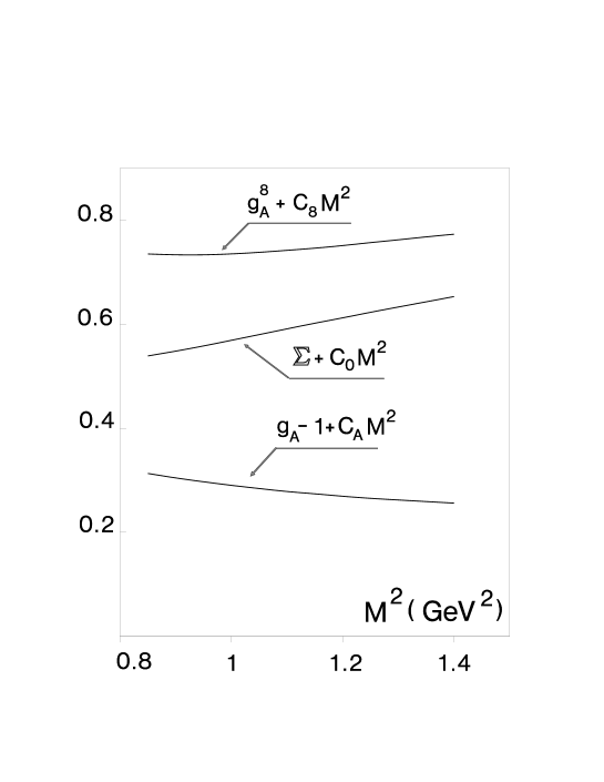This fixes the interval $0.85<M^{2}<1.4~{}GeV^{2}$.The $M^{2}$-dependence of the rhs of (25) at $f^{2}_{0}=3\times 10^{-2}~{}GeV^{2}$ is plotted in Fig.1. The complicated expression in rhs of (25) is indeed an almost linear function of $M^{2}$ in the given interval! This fact strongly supports the reliability of the approach. The best values of $\Sigma=\Sigma^{fit}$ and $C_{0}=C^{fit}_{0}$ are found from the $\chi^{2}$ fitting procedure

$$\chi^{2}=\frac{1}{n}\sum\limits^{n}_{i=1}~{}[\Sigma^{fit}+C^{fit}_{0}M^{2}_{i}-R(M^{2}_{i})]^{2}=min,$$ (27)

where $R(M^{2})$ is the rhs of (25).

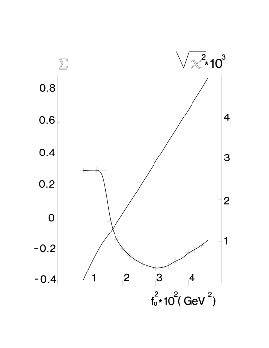
The values of $\Sigma$ as a function of $f^{2}_{0}$ are plotted in Fig.2 together with $\sqrt{\chi^{2}}$. In the used above approach the gluonic contribution cannot be separated and is included in $\Sigma$. As discussed in Sec. 1 the experimental value of $\Sigma$ can be estimated as $\Sigma=0.3\pm 0.1$. Then from Fig.2 we have $f^{2}_{0}=(2.8\pm 0.7)\times 10^{-2}~{}GeV^{2}$ and $\chi^{\prime}(0)=(2.3\pm 0.6)\times 10^{-3}~{}GeV^{2}$ . The error in $f^{2}_{0}$ and $\chi^{\prime}$, besides the experimentall error, includes the uncertainty in the sum rule estimated as equal to the contribution of the last term in OPE (two last terms in Eq.25) and a possible role of NLO $\alpha_{s}$ corrections. At $f^{2}_{0}<0.02~{}GeV^{2}$ $\chi^{2}$ is much worse and the fit becomes unstable. This allows us to claim (with some care, however,) that $\chi^{\prime}(0)\geq 1.6\times 10^{-3}GeV^{2}$ and $\Sigma\geq 0.05$ from the requirement of selfconsistency of the sum rule. The $\chi^{2}$ curve also favours an upper limit for $\Sigma\mathrel{\mathchoice{\lower 3.6pt\vbox{\halign{$\mathsurround=0pt\displaystyle\hfil#\hfil$\cr<\crcr\sim\crcr}}}{\lower 3.6pt\vbox{\halign{$\mathsurround=0pt\textstyle\hfil#\hfil$\cr<\crcr\sim\crcr}}}{\lower 3.6pt\vbox{\halign{$\mathsurround=0pt\scriptstyle\hfil#\hfil$\cr<\crcr\sim\crcr}}}{\lower 3.6pt\vbox{\halign{$\mathsurround=0pt\scriptscriptstyle\hfil#\hfil$\cr<\crcr\sim\crcr}}}}0.6$. At $f^{2}_{0}=2.8\times 10^{-2}~{}GeV^{2}$ the value of the constant $C_{0}$ found from the fit is $C_{0}=0.19~{}GeV^{-2}$. Therefore, the mentioned above necessary condition of the sum rule validity is well satisfied.

Let us discuss the role of various terms of OPE in the sum rules (25) To analyze it we have considered sum rules (25) for 4 different cases, i.e. when we take into consideration: a) only contribution of the operators up to d=3 (the term –1 and the term, proportional to $f^{2}_{0}$ in (25)); b) contribution of the operators up to d=5 (the term $\sim h_{0}$ is added); c) contribution of the operators up to d=7 (three first terms in (25)), d) our result (25), i.e. all operators up to d=9. For this analysis the value of $f^{2}_{0}=0.03~{}GeV^{2}$ was chosen, but the conclusion appears to be the same for all more or less reasonable choice of $f^{2}_{0}$. Results of the fit of the sum rules are shown in Table 3 for all four cases. The fit is done in the region of Borel masses $0.9<M^{2}<1.3~{}GeV^{2}$. In the first column the values of $\Sigma$ are shown , in the second - values of the parameter C, and in the third - the ratio $\gamma=|\sqrt{\chi^{2}}/\Sigma|$, which is the real parameter, describing reliability of the fit. From the table one can see, that reliability of the fit monotonously improves with increasing of the number of accounted terms of OPE and is quite satisfactory in the case $d$

Recently, the first attempt to calculate $\chi^{\prime}(0)$ on the lattice was performed [33]. The result is $\chi^{\prime}(0)=(0.4\pm 0.2)\times 10^{-3}~{}GeV^{2}$, much below our value. However, as mentioned by the authors, the calculation has some drawbacks and the result is preliminary.

In the papers by Narison, Shore and Veneziano (NSV) [34],[35], an attempt to find the links between $\Sigma$ and $\chi^{\prime}(0)$ was done. NSV found that $\Sigma$ is proportional to $\sqrt{\chi^{\prime}(0)}$ and calculated $\chi^{\prime}(0)$ by QCD sum rules. From my point of view, the approach of ref.’s [33],[34] is not justifiable. Instead of use of firmly based and self consistent OPE, as was done above, in [34],[35] the matrix element $<p\mid Q_{5}\mid p>$ was saturated by contribution of two operators $Q_{5}$ and singlet pseudoscalar operator $\Sigma\bar{q}\gamma_{5}q$ – and the result was obtained by orthogonalization of the corresponding matrix. I have doubts that such procedure can be grounded. The calculation of $\chi^{\prime}(0)$ by QCD sum rules is not correct, because, as was shown in [22] by considering in the same problem with account of higher order terms of OPE, than it was done in [34],[35], the OPE breaks down at the scales, characteristic for this problem. I do not believe, that the value $\chi^{\prime}(0)=(0.5\pm 0.2)\cdot 10^{-3}~{}GeV^{2}$ found in [34] is reliable.

3. Calculation of proton axial coupling constant $g^{8}_{A}$ and $g_{A}$.

From the same sum rule (25) it is possible to find $g^{8}_{A}$ – the proton coupling constant with the octet axial current, which enters the QCD formula for $\Gamma_{p,n}$. There are two differences in comparison with (25):

I. Instead of $f^{2}_{0}$ it appears the square $f^{2}_{8}$ of the pseudoscalar meson coupling constant with the octet axial current. In the limit of strict SU(3) flavour symmetry it is equal to $f^{2}_{\pi}$, $f_{\pi}=133~{}MeV$. However, it is known, that SU(3) symmetry is violated and the kaon decay constant, $f_{K}\approx 1.22f_{\pi}$ [6]. In the linear in $s$-quark mass $m_{s}$ approximation $f_{\eta}=1.28f_{\pi}$. We put for $f^{2}_{8}$ the value $f^{2}_{8}=2.6\times 10^{-2}~{}GeV^{2}$, intermediate between $f^{2}_{\pi}$ and $f^{2}_{\eta}$ .

2. $h_{0}$ should be substituted by $m^{2}_{1}f^{2}_{\pi}$. The constant $m^{2}_{1}$ is determined by the sum rules suggested in [36]. A new fit corresponding to the values of the parameters used above, was performed and it was found; $m^{2}_{1}=0.16~{}GeV^{2}$.

The $M^{2}$ -dependence of $g^{8}_{A}+C_{8}M^{2}$ is presented in Fig.1 and the best fit according to the fitting procedure (27) at $1.0\leq M^{2}\leq 1.3~{}GeV^{2}$ gives

$$g^{8}_{A}=0.65\pm 0.15,~{}~{}~{}C_{8}=0.10~{}GeV^{-2}~{}~{}~{}\sqrt{\chi^{2}}=1.2\times 10^{-3}$$ (28)

(The error includes the uncertainties in the sum rule as well as in the value of $f^{2}_{8}$). The obtained value of $g^{8}_{A}$ within the errors coincides with $g^{8}_{A}=0.59\pm 0.02$ [12] found from the data on baryon octet $\beta$-decays under assumption of strict SU(3) flavour symmetry and contradicts the hypothesis of bad violation of SU(3) symmetry in baryon axial octet coupling constants [37].

A similar sum rule with the account of dimension 9 operators can be derived also for $g_{A}$ – the nucleon axial $\beta$-decay coupling constant. It is an extension of the sum rule found in [25] and has the form

$$g_{A}+C_{A}M^{2}=1+\frac{8}{9\tilde{\lambda}^{2}_{N}}e^{m^{2}/M^{2}}\Biggl{[}a^{2}L^{4/9}+2\pi^{2}m^{2}_{1}f^{2}_{\pi}M^{2}-\frac{1}{4}a^{2}\frac{m^{2}_{0}}{M^{2}}+\frac{5}{3}\pi\alpha_{s}f^{2}_{\pi}\frac{a^{2}}{M^{2}}\Biggr{]}$$ (29)

The main term in OPE of dimension 3 proportional to $f^{2}_{\pi}$ occasionally was cancelled. For this reason the higher order terms of OPE may be more important in the sum rule for $g_{A}$ than in the previous ones. The $M^{2}$ dependence of $g_{A}-1+C_{A}M^{2}$ is plotted in Fig.1, lower curve; the curve is almost the straight line, as it should be. The best fit gives

$$g_{A}=1.37\pm 0.10,~{}~{}~{}C_{A}=-0.088~{}GeV^{-2},~{}~{}~{}~{}\sqrt{\chi^{2}}=1.0\times 10^{-3}$$ (30)

in comparison with the world average $g_{A}=1.260\pm 0.002$ [6]. The inclusion of dimension 9 operator contribution essentially improves the result: without it $g_{A}$ would be about 1.5 and $\chi^{2}$ would be much worse.

The work was supported in part by CRDF Grant RP2-132, INTAS Grant 93-0283, RFFR Grant 97-02-16131 and Swiss Grant 7SUPJ048716.

Since in comparison with previous fit [30] of the sum rules for nucleon mass the value of QCD parameter was changed now, the new fit was performed. (In the previous calculations it was used $\Lambda=100~{}MeV$, now we take $\Lambda=200~{}MeV$.). The sum rules for chirality conserving and chirality violating parts of the polarization operator $\prod\nolimits^{(0)}(p)$ (6) defined by (3) are correspondingly

$$M^{6}E_{2}\Biggl{(}\frac{W^{2}}{M^{2}}\Biggr{)}L^{-4/9}+\frac{4}{3}a^{2}L^{4/9}+\frac{1}{4}bM^{2}E_{0}\Biggl{(}\frac{W^{2}}{M^{2}}\Biggr{)}L^{-4/9}-$$

$$-\frac{1}{3}a^{2}\frac{m^{2}_{0}}{M^{2}}=\tilde{\lambda}^{2}_{N}e^{-m^{2}/M^{2}}$$ (A.1)

$$2aM^{4}E_{1}\Biggl{(}\frac{W^{2}}{M^{2}}\Biggr{)}+\frac{272}{81}~{}\frac{\alpha_{s}(M^{2})}{\pi}~{}\frac{a^{3}}{M^{2}}-\frac{1}{12}ab=m\tilde{\lambda}^{2}_{N}e^{-m^{2}/M^{2}},$$ (A.2)

where

$$b=(2\pi)^{2}\langle 0\mid\frac{\alpha_{s}}{\pi}G^{2}_{\mu\nu}\mid 0\rangle=0.50~{}GeV^{4},$$

$$E_{2}(x)=1-(1+x+\frac{x^{2}}{2})e^{-x}$$

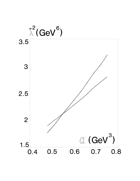
and the other notations are the same as in (25),(26). Parameters $a$ and $W^{2}$ were treated as fitting parameters and it was required that in the fitting interval $0.8<M^{2}<1.3~{}GeV^{2}$ the quantities $\tilde{\lambda}^{2}_{N}$ found from both sum rules (A.1) and (A.2) must be close to one another and close to a constant, independent of $M^{2}$. The values of $\tilde{\lambda}^{2}_{N}$, determined from (A.1) and (A.2) as functions of $a$ (at normalization point $\mu=1~{}GeV$ and continuum threshold $W^{2}=2.5~{}GeV^{2}$) are plotted on Fig.3. Two sum rules give the same value of $\tilde{\lambda}^{2}_{N}$ at $a=0.55~{}GeV^{3}$. 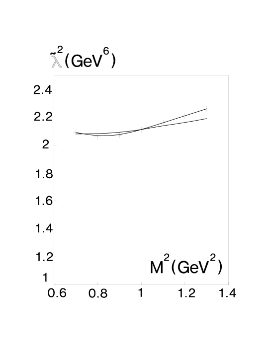The 10% variation of $W^{2}$ does not change this result. The $M^{2}$-dependence of $\tilde{\lambda}^{2}_{N}$, determined from (A.1) and (A.2) at these values of fitting parameters is shown on Fig.4. As is seen, $\tilde{\lambda}^{2}_{N}$ found from two sum rules agree with one another with accuracy $\sim 3\%$ and their deviation from constant is less than 5%. The mean value of $\tilde{\lambda}^{2}_{N}$ can be chosen as $\tilde{\lambda}^{2}_{N}=2.1~{}GeV^{6}$ $(\mu=1~{}GeV)$.

Figure Captions

Fig. 1.	The $M^{2}$-dependence of $\Sigma+C_{0}M^{2}$ at $f^{2}_{0}=3\times 10^{-2}~{}GeV^{2}$ , eq.25, $g^{8}_{A}+C_{8}M^{2}$, and $g_{A}-1+C_{A}M^{2}$, eq.29.
Fig. 2.	$\Sigma$ (solid line, left ordinate axis) and $\sqrt{\chi^{2}}$, eq.(27), (crossed line, right ordinate axis). as a functions of $f^{2}_{0}$.
Fig. 3.	The values of $\tilde{\lambda}^{2}_{N}$ as functions of $a$ determined from the sum rules (A.1) – solid line and (A.2) – crossed line.
Fig. 4.	The $M^{2}$ – dependence of $\tilde{\lambda}^{2}_{N}$ found from the sum rules (A.1) – solid line and (A.2) – crossed line.

Figure 1:

Figure 2:

Figure 3:

Figure 4:

References

[1] D.Adams et al., Phys.Rev. D56, 5330 (1997).
[2] K.Abe et al. Phys.Lett. B405, 180 (1997) .
[3] K.Ackerstaff et al., Phys.Lett. B404, 383 (1997).
[4] M.Anselmino, A.Efremov and E.Leader, Phys.Rep. 261,
1 (1995).
[5] B.L.Ioffe, Int. School of Nucleon Structure, 1st Course:
The Spin Structure of the Nucleon, Erice-Sicily, Aug.1995,
B.Frois and V.Hughes, Eds., New York, Plenum, 1997.
[6] R.M.Barnett et al., Particle Data Group, Phys.Rev.