CERN-TH/98-116

hep-ph/9804237

THERMODYNAMICS OF NON-TOPOLOGICAL SOLITONS

M. Laine^a,b and M. Shaposhnikov^a

^aTheory Division, CERN, CH-1211 Geneva 23, Switzerland
^bDepartment of Physics, P.O.Box 9, 00014 University of Helsinki, Finland

Abstract

In theories with low energy supersymmetry breaking, the effective potential for squarks and sleptons has generically nearly flat directions, $V(\phi)\sim M^{4}(\log(\phi/M))^{n}$. This guarantees the existence of stable non-topological solitons, Q-balls, that carry large baryon number, $B\gg(M/m_{p})^{4}$, where $m_{p}$ is the proton mass. We study the behaviour of these objects in a high temperature plasma. We show that in an infinitely extended system with a finite density of the baryon charge, the equilibrium state is not homogeneous and contains Q-balls at any temperature. In a system with a finite volume, Q-balls evaporate at a volume dependent temperature. In the cosmological context, we formulate the conditions under which Q-balls, produced in the Early Universe, survive till the present time. Finally, we estimate the baryon to cold dark matter ratio in a cosmological scenario in which Q-balls are responsible for both the net baryon number of the Universe and its dark matter. We find out naturally the correct orders of magnitude for $M\sim 1\ldots 10$ TeV: $\eta\sim 10^{-10}(M/{\rm TeV})^{-2}(B/10^{26})^{-1/2}$.

CERN-TH/98-116
April 1998

1 Introduction

Take a theory containing scalar fields which carry some unbroken global U(1) charge $Q$. Assume that all charged particles are massive. Suppose that the effective potential for the U(1) charged scalar fields has a flat direction, $V(\phi)\sim M^{4}$ at large $\phi$, up to possible logarithmic terms. Then this theory contains absolutely stable non-topological solitons, Q-balls, that have a non-zero value of the global charge $Q$ [1]. Flatness of the effective potential at large $\phi$ is essential for this statement. For $Q\gg 1$, the mass of the soliton grows as $M_{Q}\sim MQ^{3/4}$ and becomes smaller than the mass of a collection of free separated particles with the same charge, $mQ^{1}$, independent of the relationship between $m$ and $M$. For theories without flat directions, where $V(\phi)$ grows at large $\phi$ as $\phi^{n}$ with $n\geq 2$, Q-ball solutions constructed from scalar fields can exist as well [2, 3], but their energy scales with $Q$ as $AQ^{1}$, so that the question of their stability depends on the mass of the lightest particle that carries the charge and on the (computable) coefficient $A$.

A phenomenologically interesting example of a system with these properties is provided by supersymmetric extensions of the Standard Model. Here the role of the U(1) charge is played by the baryon number, and the role of scalar fields by squarks. The MSSM with unbroken supersymmetry has a lot of gauge invariant flat directions with $V(\phi)=0$ carrying baryon number [4]. If supersymmetry is broken at a low energy scale $M$, as in gauge-mediated scenarios [5], then the potential is lifted at $\phi>M$ in a way that $V(\phi)$ stays constant [6, 7]. Thus, this theory contains stable non-topological solitons which carry baryon number [8]. The generic MSSM with other types of SUSY breaking also contains a lot of Q-ball solutions [9, 10], but with $M_{Q}\sim MQ^{1}$.

Stable Q-balls in supersymmetric theories have a number of interesting properties. Since they represent the most economic way of packing the baryon number, they like to absorb the ordinary matter in the form of protons and neutrons and to convert baryon number from fermionic baryons to bosonic baryons (squarks) [11]. Large stable Q-balls can be naturally produced [8] in the Early Universe via the decay of an Affleck-Dine (AD) condensate [12] and can contribute to the cold dark matter [8]. Experimental signatures of relic dark matter Q-balls are spectacular [13].

At zero temperature, Q-balls are the states with minimum energy at a fixed value of the charge $Q$. They do not decay if the mass to charge ratio $M_{Q}/Q$ for them is smaller than that for a free particle. At non-zero temperatures all energy levels of the system are populated with non-zero probabilities and, thus, the charge can leak out from a Q-ball to the outer space, or, equally, can be absorbed from the surrounding plasma. Absorption of the charge into a Q-ball decreases the energy of the system, while releasing the charge from it increases the entropy. So, the issue of Q-ball stability gets more complicated than at zero temperature.

The aim of this paper is to consider Q-ball thermodynamics in theories with flat directions in the scalar potential. We will see that in these models systems with a finite density of the baryon number $n_{B}$ do not have a standard thermodynamical limit. For large enough volumes the initially homogeneous distribution of $n_{B}\neq 0$ is unstable against Q-ball formation at any temperature. On the contrary, if the volume of the system is finite and its charge is fixed, Q-balls cease to exist (evaporate completely) at temperatures $T>T_{Q}$, where $T_{Q}$ is volume dependent.

In the cosmological context, a mere thermodynamical consideration is not enough as the system has a finite time scale given by the expansion rate of the Universe, and the (non-equilibrium) rate of Q-ball evaporation is essential. We make an estimate of this rate and determine under which conditions Q-balls created in the Early Universe survive till present. If the only source of baryon asymmetry of the Universe is the AD mechanism, then the baryon asymmetry and cold dark matter may share the same origin [8]. In this scenario, both matter and dark matter are baryonic, though dark matter is constructed from squarks packed inside Q-balls. We show that in this case, the baryon to cold dark matter ratio appears to be related to very few parameters such as the charge of an individual Q-ball, the Planck scale, the SUSY breaking scale $M$ and the proton mass.

Initially, Q-balls were found and studied in different models in Refs. [1]–[3]. The generation, evolution, evaporation and implications of Q-balls at the high temperatures of the Early Universe were discussed in various models in [14]–[25]. In particular, in [19, 20] it was found that at high temperatures (but still $T\ll M$) Q-balls tend to evaporate whereas at low temperatures, they are stable and tend to grow. The influence of SUSY Q-balls on phase transitions was discussed in [23]. In theories where supersymmetry breaking comes from the supergravity hidden sector, Q-balls are unstable at zero temperature. Nevertheless, they can be produced in the Early Universe and are important for baryogenesis [24]. Moreover, they may provide a natural explanation for the ratio between neutralino dark matter and the baryonic matter in the Universe [25]. However, theories with flat potentials, specific for theories with low energy supersymmetry breaking have, to our knowledge, never been analyzed in detail for all temperatures up to $T\gg M$.

This paper is organized as follows. Essentially, it follows two distinct lines: a qualitative discussion of the physically interesting case of the MSSM with order of magnitude estimates, and a more formal and quantitative analysis, but mostly applied to a specific toy model. In Sec. 2, we formulate in general terms the main problems considered. In Sec. 3, we discuss the solutions to these problems on a qualitative level. In Sec. 4 we perform a more quantitative analysis, but in a simple renormalizable supersymmetric toy model with flat directions in the effective potential. A number of claims made in Sec. 3 are substantiated in Sec. 4. Finally, in Sec. 5 we consider the applications of the results to cosmology in the realistic case, again on an order of magnitude level. In particular, we consider here the stability of Q-balls at high temperatures, their evaporation rate, and their survival in the expanding Universe. We also estimate the baryon to cold dark matter ratio. Some details related to Sec. 4 are in the two Appendices.

2 The formulation of the problem

Let us consider a system with some conserved global charge $Q$, such as $B$ or $L$ (baryon number or lepton number; the $B+L$ anomaly is not important for this discussion).The symmetry which corresponds to this charge is assumed to be unbroken. On a formal level, the main questions we are going to address are as follows:

1. Assuming that the thermodynamical ground state of the system is homogeneous, is the conserved charge carried by individual particles in a plasma, or by a scalar condensate (Q-matter), in analogy with Bose-Einstein condensation?

2. Is such a homogeneous thermodynamical ground state stable against small inhomogeneous perturbations? If it is, is it the true ground state or a only metastable minimum?

3. In case a homogeneous ground state is unstable or metastable, what is the global minimum of the free energy? In particular, under which conditions can Q-balls constitute such a ground state?

4. If one starts from an unstable or metastable solution, at which rate does one approach the equilibrium ground state? In particular, at which rate do Q-balls form if they are stable, or evaporate if they are unstable?

In order to answer these questions, let us first fix the basic definitions used. The thermodynamics of a system with a conserved charge (the case of zero temperature is incorporated as a special case) is determined by the grand canonical partition function

$$Z_{\mu}=e^{-\beta\Omega(T,V,\mu)}=e^{\frac{V}{T}p(T,\mu)}={\rm Tr\,}e^{-\beta(\hat{H}-\mu\hat{Q})},$$ (2.1)

where

$$\frac{\left\langle\hat{Q}\right\rangle}{V}\equiv\frac{Q}{V}\equiv q=\frac{\partial p(T,\mu)}{\partial\mu}.$$ (2.2)

If $Q$ is kept fixed instead of $\mu$, then the thermodynamical potential to be minimized is obtained with a Legendre transformation:

$$F(T,V,Q)=Vf(T,q)=\Omega+\mu Q=V[-p+\mu q].$$ (2.3)

The relation inverse to eq. (2.2) is then

$$\mu=\frac{\partial f(T,q)}{\partial q}.$$ (2.4)

Given the Lagrangian of the system, one can by standard methods [26] derive a Euclidian path integral expression for $Z_{\mu}$. In a field theory containing the fields $\Phi$, it is convenient to express the result in terms of an effective action in the usual way. It then follows that

$$p(T,\mu)=-(\beta V)^{-1}\left.\Gamma_{\mu}[\Phi]\right|_{\delta\Gamma_{\mu}[\Phi]/\delta\Phi=0}.$$ (2.5)

The relevant extremum is the minimum, as follows from the general thermodynamical principle that, for fixed $T,\mu$, the other variables take such values that the corresponding free energy is minimized.

In the case of a homogeneous extremum, the problem reduces to an effective potential. Then

$$p(T,\mu)=-\left.V_{\mu}(\Phi)\right|_{dV_{\mu}/d\Phi=0}.$$ (2.6)

The Legendre transform is $V_{q}(\Phi)=V_{\mu}(\Phi)+\mu q$ where $q=-\partial_{\mu}V_{\mu}(\Phi)$, and

$$f(T,q)=\left.V_{q}(\Phi)\right|_{dV_{q}/d\Phi=0}.$$ (2.7)

With these tools, the first three of the questions formulated above can, in principle, be answered. The first of the questions is particularly straightforward: one just computes the effective potential for a fixed charge, $V_{q}(\Phi)$, and inspects whether a non-zero value for $\Phi$ serves to minimize it or not. If yes, then one can have a Q-matter condensate.

To address the second question, one can study the standard thermodynamical stability conditions: these follow from the requirement that the entropy of any subsystem must be at a maximum with respect to local fluctuations of temperature, volume, and the number of charged particles. Applied to the present case, it follows that to be stable a medium must satisfy

$$c_{V}=-T\left(\frac{\partial^{2}f}{\partial T^{2}}\right)_{q}>0;\quad\kappa_{T}=\frac{1}{q}\left(\frac{\partial p}{\partial q}\right)_{T}^{-1}>0;\quad\left(\frac{\partial\mu}{\partial q}\right)_{T}=\left(\frac{\partial^{2}f}{\partial q^{2}}\right)_{T}>0.$$ (2.8)

The last two conditions are, in fact, equivalent. The condition for $c_{V}$ is trivially satisfied in a relativistic high temperature system, since the free energy density $f$ is dominated by the term $\sim-T^{4}$. Hence essentially only the last condition remains to be inspected.

Let us note that there is an equivalent formulation for the second question. Indeed, the fluctuation matrix around the saddle point used in the evaluation of eq. (2.5) must be positive definite, from which it follows that

$$\partial_{\Phi}^{2}\left.V_{\mu}(\Phi)\right|_{\Phi=\Phi_{\rm min}}>0.$$ (2.9)

To address the third question, one has to study non-homogeneous configurations in eq. (2.5). To do this in full generality is, obviously, very difficult. However, when one restricts to spherically symmetric configurations (Q-balls), which is expected to be the relevant case, the problem becomes, to a good approximation, solvable.

Finally, the fourth question is a non-equilibrium consideration, and the tools above do not directly apply. However, the equilibrium limit turns out to give quite strong constraints. As the results depend on the initial non-equilibrium state, we will not attempt a general analysis here, but rather concentrate on the cosmologically interesting case of Q-ball evaporation in the Early Universe. This will be done in Sec. 5.

3 Q-balls at zero and finite temperatures

It turns out that the first and second questions formulated in Sec. 2, concerning the existence and stability of Q-matter, have a simple and transparent answer: a Q-matter state ($\sim$ Bose-Einstein condensate) could in principle exist, but it is unstable and will decay into an inhomogeneous configuration. We will illustrate this phenomenon in some detail in Sec. 4. In this Section we consider the inhomogeneous final state, i.e., Q-balls, in general qualitative terms. Some more details in a specific model will again be given in Sec. 4.

Let us start by reviewing the properties of Q-balls at zero temperature. Consider a generic field theory containing scalar fields $\phi_{i}$ and fermions $\psi_{i}$ with global U(1) charges $q_{i}$. The scalar potential is $V(\phi)$. Complications appearing with the inclusion of gauge fields were discussed in [27] and do not appear in the phenomenologically interesting case of SUSY theories, where flat directions are associated with SU(3)$\times$SU(2)$\times$U(1) singlets. Then, a spherically symmetric Q-ball solution has the form [1]–[3]

$$\phi_{i}(r,t)=\exp(iq_{i}\omega t)\phi_{i}(r).$$ (3.1)

The functions $\phi_{i}(r)$ can be found by minimizing the functional

$$E_{\omega}=\int d^{3}x\,\Bigl{[}\sum_{j}|\partial_{i}\phi_{j}(r)|^{2}+\hat{V}_{\omega}(\phi)\Bigr{]},$$ (3.2)

where

$$\hat{V}_{\omega}(\phi)=V(\phi)-\omega^{2}\sum_{i}q_{i}^{2}\phi_{i}^{\dagger}\phi_{i}.$$ (3.3)

The frequency $\omega$ is related to the total charge of the solution $Q$ as

$$Q=2\omega\int d^{3}x\sum_{i}q_{i}^{2}\phi_{i}^{\dagger}\phi_{i}.$$ (3.4)

Consider now the finite temperature case and a large but finite volume V. The thermodynamics of the system is determined by the grand canonical partition function defined in eq. (2.1).

Given the Lagrangian of the system, which contains all the fields of the theory, one can derive a Euclidian path integral expression for $Z_{\mu}$,

$$Z_{\mu}=\int{\cal D}[{\rm All~{}fields}]\exp\left(-\int_{0}^{\beta}\!d\tau\int\!d^{3}x{\cal L}_{E}\right),$$ (3.5)

where ${\cal L}_{E}$ is the ordinary Euclidean action with the replacement of the Euclidian time derivative  [26]

$$\partial_{\tau}\rightarrow\partial_{\tau}-q_{i}\mu.$$ (3.6)

Note that for scalar fields, the charges come with the opposite signs in $\partial_{\tau}\phi,\partial_{\tau}\phi^{\dagger}$. As usual, bosonic fields are periodic, while fermionic fields are anti-periodic on the finite time interval $0<\tau<\beta=1/T$.

To define if there are any non-trivial contributions to the partition function, potentially associated with Q-balls, one can look for the saddle points of the exponential in eq. (3.5). The configurations that play the most important role at high temperatures are static, i.e., independent of Euclidian time. The static bosonic part of the action has the form

$$S=\beta\int d^{3}x\,\Bigl{[}\sum_{j}|\partial_{i}\phi_{j}(r)|^{2}+V(\phi)-\mu^{2}\sum_{i}q_{i}^{2}\phi_{i}^{\dagger}\phi_{i}\Bigr{]},$$ (3.7)

precisely the one given by eqs. (3.2), (3.3) with the replacement $\omega\rightarrow\mu$. Thus, if the theory at zero temperature has Q-ball solutions with some values of $\omega$, these solutions are saddle points of the Euclidian finite temperature and finite density path integral at $\mu=\omega$. The relationship between the charge and $\mu$ is now given by eq. (2.2), rather than eq. (3.4): besides Q-balls, at non-zero temperatures charge can be carried by particles outside it, as well.

As is very well known from the study of phase transitions at high temperatures, the saddle points of the tree-level static bosonic action provide a good approximation only when $T\ll M$, where $M$ is the typical mass scale of the theory. At $T\mathop{\raise 1.29167pt\hbox{$>$\kern-7.5pt\raise-4.73611pt\hbox{$\sim$}}}M$, the quantum corrections are large, and must be resummed in some way. Thus one either has to use an approximation for the full effective action $\Gamma[\Phi]$ in eq. (2.5), or one has to use an effective theory where quantum corrections are small. The latter could be constructed for static but space dependent bosonic configurations, integrating out all fermions, all heavy (mass $\gg T$) bosons, and the non-zero Matsubara frequencies of light bosons. For static bosonic configurations, depending on space coordinates only weakly (we will see that this is indeed the case for sufficiently large Q-balls), the derivative expansion is most helpful:

$$S_{\rm eff}=\beta\int d^{3}x\,\Bigl{[}\sum_{j}Z_{j}(\phi,T,\mu)|\partial_{i}\phi_{j}(r)|^{2}+V_{\rm eff}(\phi,T,\mu)+...\Bigr{]},$$ (3.8)

where $V_{\rm eff}(\phi,T,\mu)$ is basically the effective potential of the system at non-zero $T$ and $\mu$ (more precisely, $V_{\rm eff}$ is the contribution to the effective potential from the degrees of freedom that have been integrated out). The effective potential as a function of $\mu$ has been computed in a number of theories and discussed in connection with the question of the influence of charge density on the symmetry behaviour in a number of papers [28]–[30]. If the particle masses in the background of the field $\phi$ are smaller than the temperature, then the high temperature expansion can be used for the construction of the effective action precisely along the lines of Refs. [31]–[34]. If not (as is in fact for many of the considerations below), then an effective action incorporating both high and low temperature behaviour must be used. Now, we have at hands enough for a qualitative discussion and order of magnitude estimates of the properties of SUSY Q-balls at high temperatures. For this aim we take the wave function normalizations in eq. (3.7) to be unity. As a number of studies [35, 31] show, higher order corrections in the wave function normalizations are not essential numerically.

Let us take some field $\phi$ representing, in somewhat loose terms, a gauge-invariant combination of squarks and sleptons in the MSSM, and carrying baryon (and, perhaps, lepton) number (for simplicity, we take the charge $q=1$). Specific examples can be found in [4]. Under the global baryon symmetry, the field $\phi$ is transformed as $\phi\rightarrow\exp(i\alpha)\phi$. Assume that the effective potential is flat along this direction as shown in Fig. 1,

$$V(\phi)\rightarrow M^{4}$$ (3.9)

at $\phi\rightarrow\infty$. Then, at zero temperature the minimum of the energy at a fixed baryonic charge $Q\gg 1$ corresponds to a time dependent Q-ball solution which can in the limit of a large charge be written as

$$\phi(r)\approx\exp(i\omega t)\times\left\{\begin{array}[]{ll}\phi_{Q}(\sin\omega r)/\omega r,&r<R_{Q}\\ &\\ 0,&r\geq R_{Q}.\end{array}\right.$$ (3.10)

Here

$$R_{Q}\approx(1/\sqrt{2})\,M^{-1}\,Q^{1/4},~{}\phi_{Q}\approx(1/\sqrt{2})\,M\,Q^{1/4},~{}\omega R_{Q}\approx\pi,$$ (3.11)

and the mass of the solution is

$$M_{Q}\approx(4\pi\sqrt{2}/3)\,M\,Q^{3/4}.$$ (3.12)

A Q-ball is stable (cannot decay into protons: $M_{Q}<m_{p}Q$) if $Q>10^{15}(M/1{\rm TeV})^{4}$.

Let us now see what happens at high temperatures. The scalar field $\phi$ couples to the other fields of the MSSM. In the background of this field a number of particles (e.g. gluons and gluinos) acquire masses $m(\phi)\sim g\phi$, while others do not (e.g. if the Q-ball solution at $T=0$ is constructed from squarks only, leptons and sleptons remain massless since they do not have tree level interactions with squarks). Now, if $g\phi>T$, massive particles do not contribute to the finite temperature effective potential just because of the Boltzmann suppression $\exp(-m(\phi)/T)$, whereas the contribution of the massless particles is $\phi$ independent and produces just an overall shift of the effective potential which we discard. At the same time, $m(\phi)$ is small near $\phi=0$. Thus, the point $\phi=0$ moves down as $\Delta V\sim-NT^{4}$, where the coefficient $N$ is related to the difference between the number of light degrees of freedom at small and large $\phi$. So, the finite temperature effective potential has qualitatively the same form as the effective potential at zero temperature, with the change $M^{4}\rightarrow M(T)^{4}\sim M^{4}+NT^{4}$.

This consideration allows to write down immediately the Q-ball contribution to the thermodynamic potential. Replacing $M_{Q}\to F_{Q}$, $M\to M(T)$ in eq. (3.12) and using that $Q^{1/4}\sim R_{Q}M\sim M/\omega\sim M/\mu$, we get

$$F_{Q}(\mu)\sim M(T)\left(\frac{M(T)}{\mu}\right)^{3},$$ (3.13)

with the charge in the Q-ball

$$Q_{Q}(\mu)\sim\left(\frac{M(T)}{\mu}\right)^{4}.$$ (3.14)

The size of the Q-ball is given by $R_{Q}\sim\pi/\mu$.

Now, the $\mu$-dependent part of the thermodynamic potential has the form

$$\Omega(T,V,\mu)=F_{Q}(\mu)-C\frac{1}{2}\mu^{2}T^{2}V,$$ (3.15)

where the coefficient $C$ is related to the number of light carriers of the baryon charge (such as quarks). The total charge of the system follows from eq. (2.2),

$$Q_{\rm total}=Q_{Q}(\mu)+C\mu T^{2}V.$$ (3.16)

These two equations define equilibrium Q-ball properties at high temperatures.

Let us assume first that the average charge density $n_{Q}$ is nonzero and is fixed, while the volume of the system grows. Then eq. (3.16) admits two solutions. The first one is with a “large” chemical potential $\mu\sim n_{Q}/(CT^{2})$. It corresponds to a state where all the charge is carried by particles in the plasma and Q-balls are not present. Another solution has a “small” chemical potential,

$$\mu\sim M(T)(n_{Q}V)^{-1/4}.$$ (3.17)

It corresponds to a system containing one Q-ball that carries almost all of the charge $Q_{\rm total}=n_{Q}V$.

Constructing the Legendre transform of eq. (3.15) according to eq. (2.3), it can now be seen that the latter solution has a smaller free energy at large volumes. Indeed, the Q-ball free energy scales with volume only as $F_{Q}\sim V^{3/4}$, whereas the free energy of the plasma phase grows as $F_{\rm plasma}\sim V$. Thus, we arrive at the conclusion that in theories with flat potentials and a fixed non-zero density of the charge $Q$, the ground state of the system always contains just one Q-ball at any temperature when $V\rightarrow\infty$.

Let us then take another limit, where the total charge of the system is fixed, and we increase its volume. In this case, the average density of the charge decreases as $n_{Q}\sim Q_{\rm total}/V$. Then, a state with a Q-ball is more favourable than a homogeneous distribution of the charge at

$$V\mathop{\raise 1.29167pt\hbox{$<$\kern-7.5pt\raise-4.73611pt\hbox{$\sim$}}}\frac{Q_{\rm total}^{5/4}}{M(T)T^{2}}.$$ (3.18)

This inequality allows, for example, an estimate of the temperature $T_{\rm evap}$ at which an initially cold Q-ball, placed in a volume $V$, evaporates. It follows from eq. (3.18) that $T_{\rm evap}\sim V^{-1/3}Q^{5/12}$, provided $T_{\rm evap}\gg M$, and $T_{\rm evap}\sim(VM)^{-1/2}Q^{5/8}$ in the opposite case.

All these results have a simple physical meaning. Imagine that we place a Q-ball at zero temperature into a box with the volume $V$. Now, let us heat the system gradually without adding any charge to it. Some charge from the Q-ball ($\delta Q$) will evaporate, and it will create a chemical potential in the surrounding plasma, $\mu_{\rm plasma}\sim\delta Q/(VT^{2})$. The process of Q-ball evaporation will stop when the chemical potential associated with the Q-ball, $\mu_{Q}\sim M(T)(Q-\delta Q)^{-1/4}$, will be equal to $\mu_{\rm plasma}$. If the inequality in eq. (3.18) is satisfied, then one finds that the solution for $\delta Q$ is

$$\frac{\delta Q}{Q}\sim\frac{M(T)VT^{2}}{Q^{5/4}}\ll 1,$$ (3.19)

so that the Q-ball cannot evaporate completely, whereas if eq. (3.18) is not true, then the equation $\mu_{\rm plasma}=\mu_{Q}$ does not have physical solutions with $Q-\delta Q\gg 1$, and therefore, the Q-ball disappears.

As we see, the structure of the ground state is obviously volume dependent. Thus, the system we consider does not have a standard thermodynamic limit. The flatness of the potential is essential for these conclusions. If $F_{Q}\sim Q^{1}$ rather than $F_{Q}\sim Q^{3/4}$, then the standard thermodynamical limit is well defined, and Q-balls cease to exist above some temperature which is entirely determined by the density of the charge and the parameters of the model.

4 A model computation

In order to illustrate in more specific terms the issues discussed above, we will in this Section consider in some detail the renormalizable model introduced in [6] for studying supersymmetric inflation. We first discuss the stability of Q-matter, and then that of Q-balls, adding numerical coefficients to the estimates in Sec. 3.

The model is defined by a superpotential with two complex fields $\phi,\chi$:

$$W={\frac{1}{2}}f\chi\phi^{2}-\chi m^{2}.$$ (4.1)

The parameters $f,m^{2}$ can be assumed to be real. We denote $\tilde{m}^{2}=fm^{2}$. In the direction of the charged field, the potential of the model grows only logarithmically. Let us assume that there are no local symmetries and thus no gauge fields.

We start by writing down the Minkowskian Lagrangian. Let us split $\phi$ to real components, $\phi=(\phi_{1}+i\phi_{2})/\sqrt{2}$, and denote the Weyl spinors corresponding to $\phi,\chi$ by $\psi_{\phi}$, $\psi_{\chi}$. Then

$${\cal L}_{M} = \partial^{\mu}\phi^{*}\partial_{\mu}\phi+\partial^{\mu}\chi^{*}\partial_{\mu}\chi+i\overline{\psi}_{\phi}\overline{\sigma}^{\mu}\partial_{\mu}\psi_{\phi}+i\overline{\psi}_{\chi}\overline{\sigma}^{\mu}\partial_{\mu}\psi_{\chi}-V(\phi_{1},\phi_{2},\chi)-{\cal L}_{\psi},\hskip 14.22636pt$$ (4.2)

where

$$V(\phi_{1},\phi_{2},\chi) = {\frac{1}{2}}\tilde{m}^{2}(\phi_{2}^{2}-\phi_{1}^{2})+\frac{1}{16}f^{2}(\phi_{1}^{2}+\phi_{2}^{2})^{2}+{\frac{1}{2}}f^{2}(\phi_{1}^{2}+\phi_{2}^{2})|\chi|^{2}+\frac{\tilde{m}^{4}}{f^{2}},\hskip 14.22636pt$$ (4.3)

$${\cal L}_{\psi} = {\frac{1}{2}}f\chi\psi_{\phi}\psi_{\phi}+f\phi\psi_{\chi}\psi_{\phi}+{\rm H.c.\ }$$ (4.4)

This action has a global U(1)-symmetry,

$$\phi\to\phi,\quad\quad\chi\to e^{i\alpha}\chi,$$

$$\psi_{\phi}\to e^{-i\alpha/2}\psi_{\phi},\quad\quad\psi_{\chi}\to e^{i\alpha/2}\psi_{\chi}.$$ (4.5)

The superpotential is not symmetric and therefore the scalar fields and the corresponding fermions transform differently. The charge corresponding to the symmetry is

$$Q=\int\!d^{3}x\left[i(\chi^{*}\partial^{0}\chi-\chi\partial^{0}\chi^{*})+{\frac{1}{2}}\overline{\psi}_{\chi}\overline{\sigma}^{0}\psi_{\chi}-{\frac{1}{2}}\overline{\psi}_{\phi}\overline{\sigma}^{0}\psi_{\phi}\right].$$ (4.6)

The theory has also a discrete symmetry, $\phi\to-\phi,\psi_{\phi}\to-\psi_{\phi}$, which however does not play any role in the following.

At tree-level at zero temperature, the ground state of the system is at a broken minimum: $\chi=0,\phi_{2}=0,\phi_{1}^{2}=4\tilde{m}^{2}/f^{2},V(\phi,\chi)=0$. There supersymmetry is conserved, and the spectrum consists of four massive scalar degrees of freedom and one Dirac fermion, all with the same mass, $\sqrt{2}\tilde{m}$. On the other hand, for large values of $|\chi|$, the minimum of the potential is at $\phi_{1}=\phi_{2}=0$ and the tree-level potential does not depend on $\chi$: this is a flat direction. Along the flat direction, two scalar degrees of freedom and one Majorana fermion remain massless. The value of the potential along the flat direction is $\tilde{m}^{4}/f^{2}=m^{4}$.

Consider then $Z_{\mu}$ in eq. (2.1). According to the standard procedure [26], the Euclidian path integral expression for $Z_{\mu}$ with the charge $Q$ as given in eq. (4.6), is

$$Z_{\mu}=\int_{\rm b.c.}{\cal D}\phi{\cal D}\chi{\cal D}\psi_{\phi}{\cal D}\psi_{\chi}\exp\left(-\int_{0}^{\beta}\!d\tau\int\!d^{3}x{\cal L}_{E}\right),$$ (4.7)

where, denoting now also $\chi=(\chi_{1}+i\chi_{2})/\sqrt{2}$, the Euclidian Lagrangian is

$${\cal L}_{E} = {\frac{1}{2}}(\partial_{\tau}\phi_{1})^{2}+{\frac{1}{2}}(\partial_{\tau}\phi_{2})^{2}+{\frac{1}{2}}(\nabla\phi_{1})^{2}+{\frac{1}{2}}(\nabla\phi_{2})^{2}$$ (4.8)

$$+ {\frac{1}{2}}(\partial_{\tau}\chi_{1}-i\mu\chi_{2})^{2}+{\frac{1}{2}}(\partial_{\tau}\chi_{2}+i\mu\chi_{1})^{2}+{\frac{1}{2}}(\nabla\chi_{1})^{2}+{\frac{1}{2}}(\nabla\chi_{2})^{2}$$

$$+ \overline{\psi}_{\phi}\overline{\sigma}^{0}\left(\partial_{\tau}+\frac{\mu}{2}\right)\psi_{\phi}-i\overline{\psi}_{\phi}\overline{\sigma}^{i}\partial_{i}\psi_{\phi}$$

$$+ \overline{\psi}_{\chi}\overline{\sigma}^{0}\left(\partial_{\tau}-\frac{\mu}{2}\right)\psi_{\chi}-i\overline{\psi}_{\chi}\overline{\sigma}^{i}\partial_{i}\psi_{\chi}$$

$$+ V(\phi,\chi)+{\cal L}_{\chi}.$$

Here $V(\phi,\chi)$, ${\cal L}_{\chi}$ are from eqs. (4.3), (4.4).

We now wish to consider the functional integral for $Z_{\mu}$ in the background of $\hat{\phi}_{1},\hat{\chi}_{1}$, i.e., to compute the effective potentials $V_{\mu}(\hat{\phi}_{1},\hat{\chi}_{1})$, $V_{q}(\hat{\phi}_{1},\hat{\chi}_{1})$, defined in eqs. (2.6), (2.7). For $\chi$, choosing to consider $\chi_{1}$ is no restriction, due to the U(1) symmetry. On the other hand, we have $\phi_{2}=0$ already at the tree-level at zero temperature, so $\phi_{2}$ remains at origin for $T>0$. In the following, we denote $\hat{\phi}_{1}=\phi_{1},\hat{\chi}_{1}=\chi_{1}$.

The details of the computation of the 1-loop effective potential are discussed in Appendix A. We consider here the numerical results and their main features. To have a weakly coupled theory, we take $f=0.5$.

4.1 The stability of Q-matter

Figure 1: The projection of the effective potential on the $\chi_{1}$-axis, at different temperatures and $\mu=0$. The temperature is given in units of the mass scale $M\equiv\tilde{m}_{0}=\tilde{m}(\tilde{m}_{0})$. The thick lines indicate the regime where $\left\langle\phi_{1}\right\rangle\neq 0$: this symmetry is restored at $T/\tilde{m}_{0}\mathop{\raise 1.29167pt\hbox{$>$\kern-7.5pt\raise-4.73611pt\hbox{$\sim$}}}4.0$. For $\chi_{1}/T\mathop{\raise 1.29167pt\hbox{$<$\kern-7.5pt\raise-4.73611pt\hbox{$\sim$}}}3.5$, the effective potential is the one of the 3d effective theory in eqs. (A.20), (A.21), and for $\chi_{1}/T\mathop{\raise 1.29167pt\hbox{$>$\kern-7.5pt\raise-4.73611pt\hbox{$\sim$}}}2.5$, the one of the 4d theory in eqs. (A.23), (A.25). The scale of $\chi_{1}$ is in both cases what appears in the 3d theory: $\chi_{1}\equiv\chi_{1}^{\rm 4d}(\overline{\mu}_{T}/4)$.

Figure 2: Left: The effective potential $V_{\mu}(\chi_{1})$ at $T/\tilde{m}_{0}=5.0$, for different values of $\mu/T$. Right: The effective potential $V_{q}(\chi_{1})$ at $T/\tilde{m}_{0}=5.0$, for different values of $q/T^{3}$. Each extremum of $V_{\mu}(\chi_{1})$ corresponds to an extremum of $V_{q}(\chi_{1})$, as well, as is shown by the symbols. For $q/T^{3}>(q/T^{3})_{c}\sim 0.065$, there is a charged condensate: $\left\langle\chi_{1}\right\rangle>0$.

Figure 3: As Fig. 2, but for $T/\tilde{m}_{0}=2.0$. The thick lines indicate the regime where the symmetry is broken, $\left\langle\phi_{1}\right\rangle\neq 0$. Due to the symmetry breaking, the potentials have more structure than in Fig. 2. The critical charge density is here $(q/T^{3})_{c}\approx 0.25$. Note that the (unique) extremum of $V_{\mu}(\chi_{1})$ at $\chi_{1}>0$ is always a maximum.

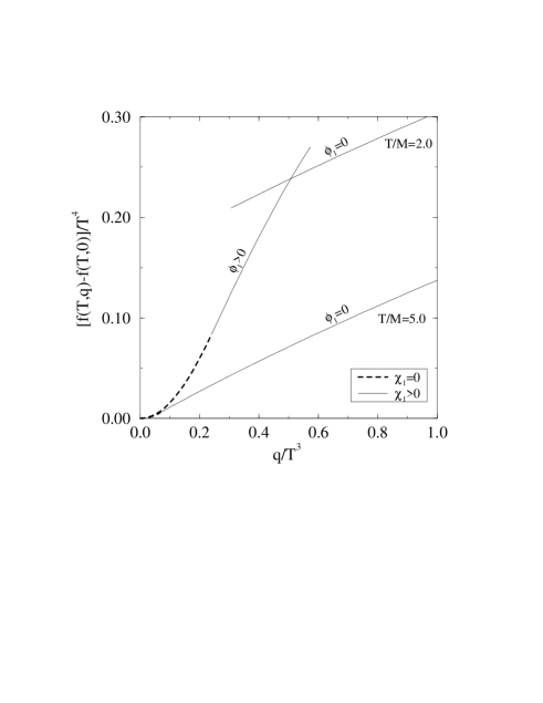
Figure 4: The free energy density as a function of the charge density for $T/\tilde{m}_{0}=2.0,5.0$. For $T/\tilde{m}_{0}\mathop{\raise 1.29167pt\hbox{$>$\kern-7.5pt\raise-4.73611pt\hbox{$\sim$}}}4$ the symmetry is always restored ($\phi_{1}=0$) and the results scale with $T$; the critical charge density below which $\chi_{1}=0$, is $(q/T^{3})_{c}\approx 0.065$. For temperatures $T/\tilde{m}_{0}\mathop{\raise 1.29167pt\hbox{$<$\kern-7.5pt\raise-4.73611pt\hbox{$\sim$}}}4$, on the other hand, the symmetry is broken ($\phi_{1}>0$) at small $\chi_{1}$, and there is more structure.

In Fig. 1, the 1-loop effective potential is shown at $\mu=0$. It is seen that for $T/\tilde{m}_{0}\mathop{\raise 1.29167pt\hbox{$>$\kern-7.5pt\raise-4.73611pt\hbox{$\sim$}}}4$, the symmetry is restored ($\phi_{1}=0$) for any $\chi_{1}$. However, irrespective of the temperature, the effective potential always displays the characteristic form allowing Q-balls: at small $\chi_{1}$, there is a thermal or vacuum mass term, but at large $\chi_{1}$, the potential flattens off and grows eventually only logarithmically.

Consider then the case of a finite charge density. In Figs. 2, 3, the potentials $V_{\mu}(\chi_{1})$ and its Legendre transform $V_{q}(\chi_{1})$ are shown at $T/\tilde{m}_{0}=5.0,2.0$, respectively. The structure is simpler at $T/\tilde{m}_{0}=5.0$, where the $\phi_{1}$-symmetry is restored everywhere and the mass scale $\tilde{m}_{0}$ does not have much effect. Nevertheless, both cases show the same general behaviour. There is a critical charge density $q_{c}>0$. For $q<q_{c}$, the minimum of $V_{q}(\chi_{1})$ is at $\chi_{1}=0$ and the charge is hence carried by particle excitations in a plasma phase. However, for $q>q_{c}$, a phenomenon analogous with Bose-Einstein condensation takes place, and $\chi_{1}>0$.

This pattern can be understood already from the tree-level potential of the effective 3d theory in eq. (A.20). Consider first the temperatures $T>T_{c}^{\phi}\approx 2\tilde{m}/f\sim 4\tilde{m}$. Then $m_{1}^{2}>0$ according to eq. (A.19), and $\phi_{1}=0$ for all $\chi_{1}$. The effective potential $V_{\mu}(\chi_{1})$ is

$$V_{\mu}(\chi_{1})\stackrel{{\scriptstyle f\chi_{1}\ll T}}{{\approx}}{\rm const.}-\frac{5}{24}\mu^{2}T^{2}+{\frac{1}{2}}\left(-\mu^{2}+\frac{f^{2}T^{2}}{8}\right)\chi_{1}^{2}.$$ (4.9)

It will be useful to consider a more general expression for the latter term in the coefficient of $\chi_{1}^{2}$, so let us replace $f^{2}T^{2}/8\to\tilde{M}^{2}$. Then the situation looks precisely like relativistic Bose-Einstein condensation in a free theory.

To proceed, let us make a Legendre transformation into $V_{q}(\chi_{1})=V_{\mu}(\chi_{1})+\mu q$, where $q=-\partial_{\mu}V_{\mu}(\chi_{1})$:

$$V_{q}\sim{\frac{1}{2}}\frac{q^{2}}{(5/12)T^{2}+\chi_{1}^{2}}+{\frac{1}{2}}\tilde{M}^{2}\chi_{1}^{2}.$$ (4.10)

What then remains is to minimize $V_{q}(\chi_{1})$ with respect to $\chi_{1}$, for different $q,T$. The main results are as follows. The global minimum is at $\chi_{1}=0$ if $\tilde{M}>(12/5)(q/T^{2})$. Hence, the critical charge density is

$$q_{c}=\frac{5}{12}\tilde{M}T^{2}.$$ (4.11)

If $q<q_{c}$, then

$$\chi_{1}=0;\quad\mu=\frac{12}{5}\frac{q}{T^{2}};\quad f(T,q)=f(T,0)+\frac{6}{5}\frac{q^{2}}{T^{2}};\quad\partial_{\chi_{1}}^{2}V_{\mu}(\chi_{1})>0.$$ (4.12)

If $q>q_{c}$, on the other hand, then

$$\chi_{1}=\sqrt{\frac{q-q_{c}}{\tilde{M}}};\quad\mu=\tilde{M};\quad f(T,q)=f(T,0)+{\frac{6}{5}}\frac{q_{c}}{T^{2}}(2q-q_{c});\quad\partial_{\chi_{1}}^{2}V_{\mu}(\chi_{1})=0.$$ (4.13)

Replacing now $\tilde{M}^{2}\to f^{2}T^{2}/8$, we see that for any given $T>T_{c}^{\phi}\sim 2\tilde{m}/f$, there is a critical charge density

$$\left(\frac{q}{T^{3}}\right)_{c}=\frac{5f}{24\sqrt{2}},$$ (4.14)

below which there is no condensate, $\chi_{1}=0$. Note that for $T>T_{c}^{\phi}$, the leading order results in eqs. (4.12), (4.13) do not depend on $\tilde{m}$ at all, and all the dimensionful quantities scale with $T$. Numerically, $(q/T^{3})_{c}\sim 0.07$, in accordance with Fig. 2.

For $T\mathop{\raise 1.29167pt\hbox{$<$\kern-7.5pt\raise-4.73611pt\hbox{$\sim$}}}T_{c}^{\phi}$, on the other hand, $m_{1}^{2}<0$ and $\phi_{1}^{2}>0$ for small $\chi_{1}$. The potential in eq. (A.20) must thus first be minimized with respect to $\phi_{1}^{2}$. After that has been done, the potential $V_{\mu}(\chi_{1})$ is again of the form in eq. (4.9) for small $\chi_{1}$, but now with $\tilde{M}^{2}=2\tilde{m}^{2}-3f^{2}T^{2}/8$. Thus the mass scale $\tilde{m}$ appears in the results. For example,

$$\left(\frac{q}{T^{3}}\right)_{c}=\frac{5}{12}\sqrt{\frac{2\tilde{m}^{2}}{T^{2}}-\frac{3f^{2}}{8}},$$ (4.15)

which gives $(q/T^{3})_{c}\sim 0.27$ for $T/\tilde{m}=2.0$, in agreement with Fig. 3.

To summarize, based on free energy considerations alone, one would say that for any temperature, there is a charge density $q_{c}$ such that for $q>q_{c}$, one has a Bose-Einstein condensate, or a “Q-matter” state. For $T\to 0$, $q_{c}\to 0$ according to eq. (4.15), and the plasma phase does not exist at all.

Let us then consider whether such a Q-matter condensate would be stable. Applying the stability conditions in eqs. (2.8), (2.9), one sees that in the tree level case, the plasma phase [eq. (4.12)] is stable while the situation in the condensate phase [eq. (4.13)] is marginal: $\partial_{q}^{2}f(T,q)=\partial_{\chi_{1}}^{2}V_{\mu}(\chi_{1})=0$. Hence the system is stabilized or destabilized through interactions. Adding an interaction of the type $\lambda(\chi^{*}\chi)^{2}$ [29, 30], in fact stabilizes the condensate. On the other hand, it is easy to see that in the present case, the interactions destabilize the condensate!

The fact that the condensate in the present system is unstable, can be observed from Figs. 2, 3. The extremum corresponding to the condensate is always a maximum of $V_{\mu}(\chi_{1})$, and thus the inequality in eq. (2.9) is violated. Equivalently, one can observe from Fig. 4 that the free energy density $f(T,q)$ has a negative curvature at $q>q_{c}$, which violates the stability condition in eq. (2.8). The negative curvature can be understood also analytically: at large charges, corresponding to large $\chi_{1}$’s,

$$V_{\mu}(\chi_{1}) \stackrel{{\scriptstyle f\chi_{1}\gg T}}{{\approx}} V_{\mu}(0)+\frac{\tilde{m}^{4}}{f^{2}}\left(1-\frac{T^{2}}{T_{c}^{\phi 2}}\right)^{2}\theta(T_{c}^{\phi}-T)$$ (4.16)

$$+ {\frac{\pi^{2}T^{4}}{24}}+\frac{\mu^{2}T^{2}}{48}-{\frac{1}{2}}\mu^{2}\chi_{1}^{2}+\frac{1}{32\pi^{2}}\tilde{m}^{4}\ln\frac{m_{\chi}^{2}}{\overline{\mu}_{T}^{2}},$$

from which it follows that

$$f(T,q) \stackrel{{\scriptstyle q\to\infty}}{{\approx}} f(T,0)+\frac{\tilde{m}^{4}}{f^{2}}\left(1-\frac{T^{2}}{T_{c}^{\phi 2}}\right)^{2}\theta(T_{c}^{\phi}-T)$$ (4.17)

$$+ \frac{\pi^{2}T^{4}}{24}+\frac{1}{16\pi^{2}}\tilde{m}^{4}\ln\left(\frac{fe^{\gamma+1/2}}{\sqrt{2}}\frac{q}{\tilde{m}^{2}T}\right).$$

Hence $\partial_{q}^{2}f(T,q)<0$. We conclude that a (meta)stable Q-matter state does not exist in the present system.

Consider then the plasma phase. That the plasma phase at $q<q_{c}$ satisfies the stability conditions in eqs. (2.8), (2.9), only proves that such a state is metastable against small perturbations. The global minimum may still be elsewhere. Consider, in particular, an arrangement where all the charge is moved into a subvolume $V^{\prime}=rV$, with $r<1$ (this of course means that there is no chemical equilibrium, but this is not essential for the argument). Let $\delta f(T,q)=f(T,q)-f(T,0)$. Then the original free energy density excess with respect to an empty space is $\delta f(T,q)$, while the final is $\delta f(T,q/r)r$. Now, for any initial $q$, $\delta f(T,q/r)r\to 0$ as $r\to 0$, since $\delta f(T,q/r)$ grows only logarithmically at small $r$, see eq. (4.17). Hence, even if $f(q/r)r$ grows at $r\mathop{\raise 1.29167pt\hbox{$<$\kern-7.5pt\raise-4.73611pt\hbox{$\sim$}}}1$ and the original state is thus metastable, $f(q/r)r$ finally starts to decrease for small enough $r$ and it is in principle favourable to clump all the charge together in one place. Of course, surface effects start to be important at very small $r$, so to be more precise, one has to inspect the possible final configurations in more detail. We thus turn to Q-balls.

4.2 The stability of Q-balls

We start by considering the limit of large temperatures, $T\gg\tilde{m}$, and small chemical potentials, $\mu\ll T$. Moreover, let us subtract the contribution of the homogeneous symmetric plasma phase, where $\chi_{1}=0$. Then it follows from eq. (A.25) that

$$\bar{V}_{\mu}(\chi_{1})\equiv V_{\mu}(\chi_{1})-V_{\mu}(0)\approx-{\frac{1}{2}}\mu^{2}\chi_{1}^{2}+\frac{T^{4}}{2\pi^{2}}\biggl{[}4J_{0}(M_{\chi}/T)-{\frac{1}{4}}J_{0}(2M_{\chi}/T)\biggr{]},$$ (4.18)

where $M_{\chi}=f\chi_{1}/\sqrt{2}$ and $J_{0}$ is from eq. (A.26). Neglecting the change in the derivative term, the extra free energy of any configuration $\chi_{1}({\bf r})$ is then given by

$$F_{\mu}=\int\!d^{3}r\left[{\frac{1}{2}}(\partial_{i}\chi_{1})^{2}+\bar{V}(\chi_{1})\right].$$ (4.19)

The properties of the saddle points of eq. (4.19) are discussed in Appendix B. It follows from eqs. (B.7), (B.8) that in the present model ($a_{V}=(\pi^{2}/24)T^{4}$), the Q-ball free energy, charge and radius at $T\gg\tilde{m}$ are given by

$$F_{Q}\approx 4.74TQ^{3/4},\quad Q\approx 160\left(\frac{\mu}{T}\right)^{-4},\quad R\approx\frac{\pi}{T}\left(\frac{\mu}{T}\right)^{-1}.$$ (4.20)

We now consider the stability of such Q-balls. The other metastable alternative is the homogeneous plasma phase, so we have to compare with $f(T,q)$ in eq. (4.12). Let us write $F_{Q}=aTQ^{3/4}$, $Q=b(\mu/T)^{-4}$.

Consider first a situation of thermal but not chemical equilibrium, in which all the charge is in the Q-ball. Then, the Q-ball does not decay into a homogeneous plasma phase, if $F_{\rm plasma}=Vf_{\rm plasma}(T,q)>F_{Q}$, or

$${\frac{6}{5}}a^{-1}Q^{5/4}>VT^{3}.$$ (4.21)

This is the analogue of eq. (3.18), and tells that in a fixed volume, Q-balls will evaporate at large enough temperatures.

On the other hand, note that what appears on the right-hand side of eq. (4.21) is a comoving volume in units of temperature, which is a constant in the cosmological context. Thus, in this case, if Q-balls are thermally stable at some high temperature, they remain stable at least as long as $T\gg\tilde{m}$. The thermal stability of a distribution of Q-balls can be seen by replacing $V$ by their inverse number density $n_{Q}^{-1}$.

Consider then a thermodynamical equilibrium situation where there is chemical equilibrium, as well. Some of the charge will now be outside the Q-ball, since there is a non-vanishing chemical potential. The stability condition becomes

$${\frac{6}{5}}\frac{Q^{2}}{VT^{3}}>{\frac{6}{5}}\frac{(Q-Q^{\prime})^{2}}{VT^{3}}+a(Q^{\prime})^{3/4},$$ (4.22)

where the Q-ball charge $Q^{\prime}$ is to be solved from an equality following from chemical equilibrium:

$$\frac{\mu}{T}\stackrel{{\scriptstyle\rm\mbox{\tiny plasma}}}{{=}}\frac{12}{5}\frac{Q-Q^{\prime}}{VT^{3}}\stackrel{{\scriptstyle\rm\mbox{\tiny Q-ball}}}{{=}}\left(\frac{Q^{\prime}}{b}\right)^{-1/4}.$$ (4.23)

However, it can easily be seen that when eq. (4.21) is strongly enough satisfied, then the fact that there is chemical equilibrium does not change the result. Indeed, it can be seen from eq. (4.23) that most of the charge resides in Q-balls in this limit,

$$\frac{Q^{\prime}}{Q}\approx 1-\frac{b^{1/4}}{2a}\left[\frac{VT^{3}}{(6/5)a^{-1}Q^{5/4}}\right]\approx 1,$$ (4.24)

and Q-balls carry most of the free energy associated with the non-zero net charge,

$$\frac{F_{\rm plasma}}{F_{Q}}\approx\frac{b^{1/2}}{4a^{2}}\left[\frac{VT^{3}}{(6/5)a^{-1}Q^{5/4}}\right]\ll 1.$$ (4.25)

Moreover, provided that the Q-ball charge is large, Q-balls are small in the sense that most of the space is in the plasma phase:

$$\frac{V_{Q}}{V_{\rm plasma}}=\frac{(4/3)\pi(R_{Q}T)^{3}}{VT^{3}}\approx\frac{10\pi^{4}a}{9b^{3/4}}\left[\frac{(6/5)a^{-1}Q^{5/4}}{VT^{3}}\right]\frac{1}{Q^{1/2}}\ll 1,$$ (4.26)

if

$$Q\gg 130\left[\frac{(6/5)a^{-1}Q^{5/4}}{VT^{3}}\right]^{2}.$$ (4.27)

Even though chemical equilibrium does not essentially change the constraint in eq. (4.21), there is an important implication following from eq. (4.23). Noting that the entropy density is $s=dp/dT=\pi^{2}T^{3}/3$, one gets a simple relation between the charge density in the plasma, and the charge residing in a Q-ball:

$$\left(\frac{q}{s}\right)_{\rm plasma}=\frac{5}{4\pi^{2}}\frac{\mu}{T}=\frac{5b^{1/4}}{4\pi^{2}}(Q^{\prime})^{-1/4}\approx 0.45(Q^{\prime})^{-1/4}.$$ (4.28)

In the cosmological context, this corresponds to a relation between the baryon asymmetry in the plasma, and the baryon number residing in Q-balls.

Finally, consider what happens at lower temperatures. The Q-ball free energy will decrease for a while as $\sim T$, until at $T\mathop{\raise 1.29167pt\hbox{$<$\kern-7.5pt\raise-4.73611pt\hbox{$\sim$}}}\tilde{m}/f$, the symmetry breaking starts to play a role: eventually $T$ gets replaced by $\tilde{m}/f^{1/2}$ in eq. (4.20). At the same time, the Q-part of the free energy of the plasma phase also decreases, initially as $F_{\rm plasma}\sim(6/5)(Q^{2}/VT^{3})T\sim T$. This behaviour is valid up to $T\sim\tilde{m}/\pi$; at smaller temperatures one gets the standard non-relativistic ideal gas behaviour $F_{\rm plasma}\sim QT[\ln Q/(VT^{3})+(3/2)\ln(T/\tilde{m})]\sim T$. Hence the plasma phase free energy decreases faster than $F_{Q}$ and a thermalized Q-ball in a comoving volume becomes more unstable at smaller temperatures.

The considerations above concern an equilibrium situation. There are also other relevant questions, such as, assuming that one is trapped in a metastable homogeneous plasma phase and Q-balls would be stable, what is the transition rate? Some progress in addressing this question has been reported in [36], but we will not consider it here. In the next Section we consider the opposite limit: taking a Q-ball which is unstable, at which rate does it decay into the plasma phase?

5 Baryon to cold dark matter ratio

Consider Q-balls in the cosmological context. In [8] it was shown that Q-balls with large charges can be produced in the Early Universe. The general idea is that in the AD scenario for baryogenesis, an uniform condensate of the scalar field, carrying baryon number, is formed as a result of inflation, CP-violation and baryon number non-conservation [12]. This AD condensate is nothing but Q-matter, described by an uniform scalar field with a time dependent phase. As we have seen, Q-matter is unstable against Q-ball formation; an analysis of the typical instability scales shows that charges of the order of magnitude $Q>10^{20}$ can be easily formed (and do not violate experimental constraints [37]). In [8] it was suggested that these stable Q-balls can play the role of the cold dark matter. The ordinary, baryonic matter appears then as a result of Q-ball evaporation. If true, baryonic and cold dark matter in the Universe come from the same source. Moreover, dark matter is in fact baryonic in this case, but baryons exist in the form of SUSY Q-balls which do not participate in nucleosynthesis. In this scenario the ratio of baryonic to cold dark matter can be computed and the aim of this Section is to make such an estimate.

We assume that after the instability has taken place, the Universe is filled with baryonic Q-balls with charge $Q$ and number density $n_{Q}$, surrounded by a hot plasma at temperature $T$. We will also assume that only a negligible part of the baryonic charge initially exists in the plasma. Some arguments if favour of this assumption were put forward in [25], but its complete check would require the solution of the non-linear problem of Q-ball formation. In the following, we completely neglect the process of merging of two Q-balls, since their concentration is so small that the probability of their collision is absolutely negligible, as can be checked a posteriori.

As a starting point, let us consider what the thermodynamical equilibrium state corresponding to these initial conditions would be. Then we will argue that in fact only thermal equilibrium can be established in practice, while chemical equilibrium with respect to baryon charge is not reached with these initial conditions.

If there is full thermodynamical equilibrium, then it follows from eq. (4.23) that already at high temperatures, the baryon to photon ratio in the plasma phase would be

$$\eta=\frac{n_{B}}{n_{\gamma}}\sim Q^{-1/4}.$$ (5.1)

In full thermal equilibrium Q-balls become more unstable at lower temperatures, see Sec. 4.2, so that with the experimental number $\eta\sim 10^{-10}$, eq. (5.1) would imply the lower bound $Q\mathop{\raise 1.29167pt\hbox{$>$\kern-7.5pt\raise-4.73611pt\hbox{$\sim$}}}10^{40}$. On the other hand, if Q-balls account for a fraction $\Omega_{\rm DM}$ of the dark matter, then their present number density is $n_{Q}^{\rm(0)}=\rho_{Q}^{\rm(0)}/M_{Q}$, where

$$\rho_{Q}^{\rm(0)}\approx 10^{-5}\Omega_{\rm DM}\,m_{p}\,{\rm cm}^{-3},$$ (5.2)

and $m_{p}$ is the proton mass. It follows that

$$n_{Q}^{-1}T^{3}\approx 3\times 10^{8}g_{*}^{-1}\frac{M}{m_{p}}\frac{Q^{3/4}}{\Omega_{\rm DM}},$$ (5.3)

where $g_{*}$ is the number of massless degrees of freedom. If, for instance, $g_{*}\sim 200,\Omega_{\rm DM}\sim 0.4,Q\sim 10^{40}$ and $M\sim(1\ldots 10)$ TeV, then $n_{Q}^{-1}T^{3}\sim 10^{39}\ldots 10^{40}$. Comparing now with the LHS of eq. (4.21), it is seen that such a density of Q-balls would indeed be thermodynamically stable against evaporation into the plasma phase. However, it is not clear how Q-balls with charges as large as $10^{40}$ could be produced, and whether they would indeed reach thermodynamical equilibrium in the cosmological environment.

Now we are going to take into account the expansion of the Universe. First of all, the intrinsic temperature of Q-balls may be different from the temperature of the surrounding plasma, if the system is not fully thermalized. Then Q-balls are heated up because of collisions with particles from the plasma. The energy transfer to the scalar particles in the condensate from which the Q-ball is built, has been estimated in [8] (we assume that all coupling constants are of order unity),

$$\frac{dF}{dt}\sim R_{Q}^{2}T^{3}\sigma n_{\phi}\delta R\delta E\sim T^{2}(\frac{T}{M})^{3}Q^{1/4}.$$ (5.4)

Here $R_{Q}^{2}T^{3}$ counts the initial flux of particles in the plasma on the Q-ball, $\delta E\sim\omega$ gives the energy transfer to a scalar particle in the condensate, $\delta R\sim T/M^{2}$ gives the thickness of the Q-ball layer in which plasma particles can penetrate (due to $m_{\phi}\sim\phi\mathop{\raise 1.29167pt\hbox{$<$\kern-7.5pt\raise-4.73611pt\hbox{$\sim$}}}T$), $n_{\phi}\sim\phi^{2}\omega\sim T^{2}MQ^{-1/4}$ is the charged scalar particle number density in this layer [eq. (3.4)], $\sigma\sim 1/(\omega T)$ is the typical cross-section of the interaction of an energetic particle from the plasma with a condensate scalar with a small energy $\sim\omega$, and we assumed $T\gg M$. The estimate in eq. (5.4) contains only the effect of particles interacting strongly (at tree-level) with the condensate, so that it should represent a lower bound of the thermalization rate.

The energy transfer is most efficient at high temperatures. Requiring that the change of Q-ball free energy is of the order of its equilibrium value $F\sim TQ^{3/4}$, we find that a zero-temperature Q-ball can be thermalized if the initial temperature of the plasma satisfies the requirement

$$T_{\rm in}>M\left(\frac{M}{M_{0}}\right)^{1/2}Q^{1/4},$$ (5.5)

where $M_{0}=(0.30/\sqrt{g_{*}})m_{\rm Pl}\sim 3\times 10^{17}$ GeV. For typical values of $M\sim 1-10$ TeV and $Q\sim 10^{20}-10^{30}$, $T_{\rm in}\mathop{\raise 1.29167pt\hbox{$>$\kern-7.5pt\raise-4.73611pt\hbox{$\sim$}}}1\ldots 10^{4}$ GeV, which is true for most inflationary models.

Next, we would like to determine the amount of baryons which evaporated from thermalized Q-balls. From the discussion in Sec. 3, we know that we can associate with Q-balls a chemical potential $\mu\sim M(T)Q^{-1/4}$. In the case that the surrounding plasma has the same chemical potential, Q-balls are in chemical equilibrium and their charge does not change. In other words, the rate of their evaporation coincides with the rate of charge accretion on the Q-ball. The upper limit on the accretion can be easily computed: the rate of accretion cannot be larger than the total baryonic flux through the Q-ball surface. So,

$$\frac{dQ}{dt}=-D(\mu_{Q}-\mu_{\rm plasma})T^{2}4\pi R_{Q}^{2}\stackrel{{\scriptstyle\mu_{\rm plasma}\ll\mu_{Q}}}{{\sim}}-D\frac{T^{2}Q^{1/4}}{M(T)},$$ (5.6)

where the coefficient $D\mathop{\raise 1.29167pt\hbox{$<$\kern-7.5pt\raise-4.73611pt\hbox{$\sim$}}}1$ shows the deviation of the real evaporation rate from the upper bound. At $T>m_{\phi}$ ($m_{\phi}$ is the mass of squarks, suppressed by some coupling constants with respect to $M$), the evaporation rate must be parametrically the same as the upper bound, since the scalar particles building up the Q-ball appear with a large number density $\sim T^{3}$ also in the plasma phase. Hence, the rate of Q-ball evaporation in a plasma with a vanishing chemical potential ($\mu_{\rm plasma}=0$) at $T>m_{\phi}$ is given by eq. (5.6) with $D\sim 1$. At $T<m_{\phi}$, the charge in the plasma sits mainly in light fermions; the probability of squark emission from a Q-ball is suppressed by the Boltzmann exponent $\exp(-m_{\phi}/T)$. Therefore, the emission of heavy squarks from the Q-ball surface can be neglected. The main process which is allowed is squark-squark transition into two quarks, $\phi\phi\rightarrow qq$. It may occur through gluino exchange with a cross-section of the order of $\sigma\sim\beta/m_{\phi}^{2}$ (see also a similar discussion in [38]), where $\beta$ is some combination of the coupling constants. Thus, we expect $D\sim\beta T^{2}/m_{\phi}^{2}$ at $T<m_{\phi}$.

By integrating eq. (5.6) (we assume a radiation dominated Universe) we find that Q-ball evaporation is negligible at $T<m_{\phi}$ ($D$ is essentially replaced by $\beta$ in eq. (5.7)). The charge $Q_{T}$ of a Q-ball at $T\sim m_{\phi}$ is related to its initial charge $Q_{0}$ as

$$Q_{T}\sim Q_{0}\left(1-D\frac{M_{0}}{MQ_{0}^{3/4}}\ln(\frac{M}{m_{\phi}})\right)^{4/3}.$$ (5.7)

Most of the charge is evaporated at low temperatures near $T\sim m_{\phi}$.

From eq. (5.7) we conclude that Q-balls survive evaporation if their initial charge is

$$Q_{0}\mathop{\raise 1.29167pt\hbox{$>$\kern-7.5pt\raise-4.73611pt\hbox{$\sim$}}}\left(D\frac{M_{0}}{M}\ln(\frac{M}{m_{\phi}})\right)^{4/3}.$$ (5.8)

If, for example, $M\sim 1$ TeV, then all Q-balls with $Q_{0}>10^{20}$ stay till the present time. It is interesting to note that these values of $Q$ are naturally produced from the decay of an AD condensate.

Now, if eq. (5.8) is satisfied, then the amount of charge evaporated from an individual Q-ball is of the order of

$$\Delta Q\sim D\frac{M_{0}}{M}\ln(\frac{M}{m_{\phi}})Q_{0}^{1/4}.$$ (5.9)

Thus, the number density of baryons $n_{B}$ in the plasma is related to the number density of Q-balls $n_{Q}$ as

$$n_{B}\sim n_{Q}\Delta Q.$$ (5.10)

Using then $n_{Q}$ from eq. (5.3) together with the entropy density $s\approx(2/45)g_{*}\pi^{2}T^{3}$, and assuming that Q-balls give all the cold dark matter in the Universe with $\Omega_{\rm DM}\sim 0.4$, the baryon to photon ratio is computable:

$$\eta=\frac{n_{B}}{n_{\gamma}}\sim 10^{-8}\frac{M_{0}m_{p}}{M^{2}Q_{0}^{1/2}}\ln(\frac{M}{m_{\phi}}).$$ (5.11)

The correct ratio $\eta\sim 10^{-10}$ appears quite naturally with the choice of, e.g., $M\sim 1-10$ TeV and a corresponding initial charge $Q_{0}\sim 10^{28}-10^{22}$. These values are quite plausible from the mechanism of Q-ball formation.

Since Q-balls interact very rarely, they should not take part in light element nucleosynthesis. From the point of view of structure formation, they are completely equivalent to weakly interacting cold dark matter. They thus behave in a somewhat similar way as quark nuggets [39].

6 Conclusions

Supersymmetric non-topological solitons in theories with flat directions of the effective potential have a number of interesting properties at high temperatures. Provided that their charge is large enough, Q-balls can exist at any temperature. Unlike for “classic” Q-balls with $M_{Q}\sim Q^{1}$, the ground state of a system with a finite density of the charge is not translationally invariant and contains Q-balls. The state of Q-matter (Bose-Einstein condensate) appears to be always unstable and it decays into Q-balls.

These properties have interesting implications for cosmology. Depending on the mechanism of Q-ball formation, thermal and chemical equilibrium may or may not be reached. If it is reached, an equilibrium distribution of Q-balls with charges $Q\mathop{\raise 1.29167pt\hbox{$>$\kern-7.5pt\raise-4.73611pt\hbox{$\sim$}}}10^{40}$ could account for both the net baryon asymmetry needed for nucleosynthesis, and for the cold dark matter. In this picture, the dark matter is in fact baryonic, with the baryon charge distributed between ordinary baryons with $n_{B}/n_{\gamma}\sim 10^{-10}$, and squarks packed inside dark matter Q-balls.

On the other hand, for charges $Q\sim 10^{22}\ldots 10^{28}$ which are more likely from the point of view of Q-ball formation, only thermal equilibrium is reached. But even then, it turns out that the right orders of magnitude for the baryon asymmetry in ordinary baryons and for the dark matter in Q-balls, can be reached provided that supersymmetry is broken at a low energy scale $M\sim 1\ldots 10$ TeV. Thus Q-balls represent an appealing candidate for the cold dark matter, offering a new picture in which the origin of ordinary baryons and the dark matter is the same.

Appendix Appendix  A: A model effective potential

In this appendix, we derive the 1-loop effective potential of the theory considered in Sec. 4 for given $\mu,T$, both at small and large values of the fields. These two cases have to be treated separately, as the theory requires a resummation for small values of the fields.

At 1-loop level, one has to consider renormalization. To be specific, the running of the fields and parameters is at 1-loop level determined by

$$\overline{\mu}\frac{d}{d\overline{\mu}}f^{2} = \frac{5}{16\pi^{2}}f^{4},\quad\quad\overline{\mu}\frac{d}{d\overline{\mu}}\tilde{m}^{2}=\frac{3}{16\pi^{2}}f^{2}\tilde{m}^{2},$$ (A.1)

$$\overline{\mu}\frac{d}{d\overline{\mu}}\phi^{*}\phi = -\frac{2}{16\pi^{2}}f^{2}\phi^{*}\phi,\quad\quad\overline{\mu}\frac{d}{d\overline{\mu}}\chi^{*}\chi=-\frac{1}{16\pi^{2}}f^{2}\chi^{*}\chi.$$ (A.2)

Here $\phi^{*}\phi$, $\chi^{*}\chi$ denote the renormalized fields squared appearing in the Lagrangian, and not any composite operators. As a result, the parameters and fields at scale $\overline{\mu}$ are

$$\phi^{*}\phi(\overline{\mu}) \approx \phi^{*}\phi(\overline{\mu}_{0})\left(\frac{\overline{\mu}}{\overline{\mu}_{0}}\right)^{-\frac{2f^{2}}{16\pi^{2}}},\quad\chi^{*}\chi(\overline{\mu})\approx\chi^{*}\chi(\overline{\mu}_{0})\left(\frac{\overline{\mu}}{\overline{\mu}_{0}}\right)^{-\frac{f^{2}}{16\pi^{2}}},$$ (A.3)

$$\tilde{m}^{2}(\overline{\mu}) \approx \tilde{m}^{2}(\overline{\mu}_{0})\left(\frac{\overline{\mu}}{\overline{\mu}_{0}}\right)^{\frac{3f^{2}}{16\pi^{2}}},\quad f^{2}(\overline{\mu})\approx\frac{16\pi^{2}}{5\ln(\Lambda/\overline{\mu})},$$ (A.4)

where $\Lambda=\overline{\mu}_{0}\exp[16\pi^{2}/5f^{2}(\overline{\mu}_{0})]$.

The theory can then be defined in terms of two parameters, the values of $\tilde{m}^{2}(\overline{\mu}_{0})$, $f(\overline{\mu}_{0})$, at some value $\overline{\mu}_{0}$ of the $\overline{\mbox{\rm MS}}$ scale parameter. We choose $\overline{\mu}_{0}\equiv\tilde{m}_{0}$, where $\tilde{m}_{0}=\tilde{m}(\tilde{m}_{0})$. Then all the dimensionful quantities, such as the temperature $T$, are measured in units of $\tilde{m}_{0}$, and the results only depend on $f(\tilde{m}_{0})$. To have a weakly coupled theory up to very high scales, we arbitrarily choose $f(\tilde{m}_{0})=0.5$.

The most convenient way to implement the resummation needed at small values of the fields, is to construct an effective 3d theory describing the thermodynamics [31]–[34]. On the other hand, for large values of $\chi$, no resummation is needed and the effective 3d theory is not valid any more. Then one can use the standard 4d finite temperature 1-loop potential. Let us discuss the 3d theory first.

A.1 The 3d effective theory and $V(\phi,\chi)$ at small $\phi,\chi$

Let us denote

$$M_{\phi}=\frac{1}{\sqrt{2}}f\phi_{1},\quad M_{\chi}=\frac{1}{\sqrt{2}}f\chi_{1}.$$ (A.5)

The effective theory constructed is valid for $M_{\phi},M_{\chi}\ll\pi T$, and implements the resummation needed in the regime $M_{\phi,\chi}\mathop{\raise 1.29167pt\hbox{$<$\kern-7.5pt\raise-4.73611pt\hbox{$\sim$}}}fT$.

The derivation of the effective theory proceeds by computing the $n$-point functions in the original theory and in the effective theory, and by matching the parameters of the effective theory such that the original results are reproduced. In the present context, one has to consider the 2-point functions of the bosonic fields at non-zero momenta to get the field normalizations, and the 2- and 4-point functions at zero momenta. The field normalizations arise from fermionic loops alone. The zero-momentum correlators arise both from bosonic and fermionic loops, and the most convenient way of deriving them is the effective potential, expanded in terms of masses to the required order. We will also expand in $\mu$, assuming $\mu\ll\pi T$, although this would not be necessary. We then assume that parametrically $f\phi,f\chi,\mu\sim fT$ and work at 1-loop level to order $f^{4}$. Thus we need the first five terms (up to $B^{4}$) from the expansion

$${\frac{1}{2}}\ln\det(A+B)={\frac{1}{2}}\ln\det A+\sum_{n=1}^{\infty}\frac{(-1)^{n+1}}{2n}{\rm Tr\,}(A^{-1}B)^{n}.$$ (A.6)

In the bosonic case, the matrices are

$$A^{-1} = \frac{1}{p^{2}}\mathop{\rm diag}(1,1,1,1),$$

$$B = \left(\begin{array}[]{cccc}\tilde{m}^{2}+{\frac{1}{2}}M_{\phi}^{2}+M_{\chi}^{2}&0&0&0\\ 0&-\tilde{m}^{2}+{\frac{3}{2}}M_{\phi}^{2}+M_{\chi}^{2}&2M_{\phi}M_{\chi}&0\\ 0&2M_{\phi}M_{\chi}&-\mu^{2}+M_{\phi}^{2}&-2\mu p_{0}\\ 0&0&2\mu p_{0}&-\mu^{2}+M_{\phi}^{2}\end{array}\right),\hskip 28.45274pt$$ (A.11)

where $p^{2}=p_{0}^{2}+{\bf p}^{2}$ and $p_{0}$ is a bosonic Matsubara frequency. In the fermionic case,

$$A^{-1}=\frac{1}{p^{2}}\left(\begin{array}[]{cc}-i/\!\!\!p&0\\ 0&-i/\!\!\!p\end{array}\right),\quad B=\left(\begin{array}[]{cc}-\frac{\mu}{2}\gamma_{0}\gamma_{5}+M_{\chi}&M_{\phi}\\ M_{\phi}&\frac{\mu}{2}\gamma_{0}\gamma_{5}\end{array}\right).$$ (A.12)

The fermionic matrices have been written in the basis of the Majorana fermions

$$\tilde{\psi}_{\phi}=\left(\begin{array}[]{c}\psi_{\phi}\\ \overline{\psi}_{\phi}\end{array}\right),\quad\tilde{\psi}_{\chi}=\left(\begin{array}[]{c}\psi_{\chi}\\ \overline{\psi}_{\chi}\end{array}\right),$$ (A.13)

where we used the standard notation of Ref. [40]. There is an overall minus sign in eq. (A.6) for fermions, and only even powers of $B$ contribute due to the momentum integration.

The basic integrals appearing in the evaluation of the traces are

$${\hbox{$\sum$}\!\!\!\!\!\!\int}_{\!\!\!\!p_{b}}^{\prime}\frac{1}{p^{2}}=\frac{T^{2}}{12},\quad{\hbox{$\sum$}\!\!\!\!\!\!\int}_{\!\!\!\!p_{b}}^{\prime}\frac{1}{(p^{2})^{2}}=\frac{1}{16\pi^{2}}\left[\frac{1}{\epsilon}+L_{b}(\overline{\mu})\right],\quad{\hbox{$\sum$}\!\!\!\!\!\!\int}_{\!\!\!\!p_{b}}^{\prime}\frac{1}{(p^{2})^{3}}=\frac{\zeta(3)}{128\pi^{4}T^{2}},$$ (A.14)

$${\hbox{$\sum$}\!\!\!\!\!\!\int}_{\!\!\!\!p_{f}}\frac{1}{p^{2}}=-\frac{T^{2}}{24},\quad{\hbox{$\sum$}\!\!\!\!\!\!\int}_{\!\!\!\!p_{f}}\frac{1}{(p^{2})^{2}}=\frac{1}{16\pi^{2}}\left[\frac{1}{\epsilon}+L_{f}(\overline{\mu})\right],\quad{\hbox{$\sum$}\!\!\!\!\!\!\int}_{\!\!\!\!p_{f}}\frac{1}{(p^{2})^{3}}=\frac{7\zeta(3)}{128\pi^{4}T^{2}},\hskip 14.22636pt$$ (A.15)

where $p_{b},p_{f}$ are the bosonic and fermionic Matsubara momenta, a prime means that the zero Matsubara mode is omitted, and

$$L_{b}(\overline{\mu})=2\ln\frac{\overline{\mu}}{\overline{\mu}_{T}},\quad L_{f}(\overline{\mu})=2\ln\frac{4\overline{\mu}}{\overline{\mu}_{T}},\quad\overline{\mu}_{T}=4\pi e^{-\gamma}T.$$ (A.16)

The other integrals appearing, of the form $\int\!\!\!\!\!\raise-0.86108pt\hbox{$\Sigma$}\,(p_{0}^{2})^{n}/(p^{2})^{m}$, can be derived from those in eq. (A.15) by taking derivatives with respect to $T$.

As a result, the 3d finite temperature effective theory describing the thermodynamics of the original 4d theory is defined by the action

$$S_{\rm 3d} = \frac{V}{T}\left[-\frac{\pi^{2}}{12}T^{4}-\frac{5}{24}\mu^{2}T^{2}+\frac{7}{192\pi^{2}}\mu^{4}+\frac{\tilde{m}^{4}(\overline{\mu}_{T})}{f^{2}(\overline{\mu}_{T})}\right]$$ (A.17)

$$+ \int\!d^{3}x\,\biggl{[}{\frac{1}{2}}(\nabla\phi_{1})^{2}+{\frac{1}{2}}(\nabla\phi_{2})^{2}+(\nabla\chi)^{*}(\nabla\chi)$$

$$+{\frac{1}{2}}m_{1}^{2}\phi_{1}^{2}+{\frac{1}{2}}m_{2}^{2}\phi_{2}^{2}+m_{\chi}^{2}\chi^{*}\chi$$

$$+{\frac{1}{4}}\lambda_{\phi}(\phi_{1}^{2}+\phi_{2}^{2})^{2}+{\frac{1}{2}}\lambda_{m}(\phi_{1}^{2}+\phi_{2}^{2})\chi^{*}\chi+\lambda_{\chi}(\chi^{*}\chi)^{2}\biggr{]}.$$

Here the fields are related to the 4d fields by

$$(\phi\phi)_{\rm 3d}=\frac{1}{T}(\phi\phi)_{\rm 4d}\Bigl{(}{\frac{1}{4}}\overline{\mu}_{T}\Bigr{)},\quad(\chi\chi)_{\rm 3d}=\frac{1}{T}(\chi\chi)_{\rm 4d}\Bigl{(}{\frac{1}{4}}\overline{\mu}_{T}\Bigr{)}.$$ (A.18)

The parameters are given by

$$m_{1}^{2} = -\tilde{m}^{2}\left(2^{-4/3}\overline{\mu}_{T}\right)-\frac{f^{2}\mu^{2}}{16\pi^{2}}+\frac{f^{2}T^{2}}{4},$$

$$m_{2}^{2} = \tilde{m}^{2}\left(2^{-4/3}\overline{\mu}_{T}\right)-\frac{f^{2}\mu^{2}}{16\pi^{2}}+\frac{f^{2}T^{2}}{4},$$

$$m_{\chi}^{2} = -\mu^{2}\left(1-\frac{f^{2}}{16\pi^{2}}\right)+\frac{f^{2}T^{2}}{8},$$

$$\lambda_{\phi} = {\frac{1}{4}}Tf^{2}\left(2^{8/5}\overline{\mu}_{T}\right),\quad\lambda_{m}=Tf^{2}\left(2^{2/5}\overline{\mu}_{T}\right),\quad\lambda_{\chi}=T\frac{f^{4}}{8\pi^{2}}\ln 2.$$ (A.19)

Note, in particular, that around the two “symmetry restoring” temperatures [$T_{c}^{\phi}=2\tilde{m}/f$ where $m_{1}^{2}\sim 0$, and $T_{c}^{\chi}=2\sqrt{2}\mu/f$ where $m_{\chi}^{2}\sim 0$], one has $\pi T\gg\{\tilde{m},\mu\}$ for a small coupling $f$, so that the construction of the effective theory is well convergent.

To go further with resummed perturbation theory, one can compute the effective potential in the theory defined by the action in eq. (A.17). The general pattern can be seen already from the tree-level potential,

$$V_{\rm tree}={\rm const.}+{\frac{1}{2}}m_{1}^{2}\phi_{1}^{2}+{\frac{1}{2}}m_{\chi}^{2}\chi_{1}^{2}+{\frac{1}{4}}\lambda_{\phi}\phi_{1}^{4}+{\frac{1}{4}}\lambda_{m}\phi_{1}^{2}\chi_{1}^{2}+{\frac{1}{4}}\lambda_{\chi}\chi_{1}^{4}.$$ (A.20)

This tree-level potential of the 3d theory corresponds to the dominant thermal screening contributions in the 4d 1-loop potential. The 3d 1-loop correction is

$$V_{\rm 1-loop}=-\frac{1}{12\pi}\sum_{i=\phi_{2},\chi_{2},\pm}m_{i}^{3},$$ (A.21)

where

$$m_{\phi_{2}}^{2} = m_{2}^{2}+\lambda_{\phi}\phi_{1}^{2}+{\frac{1}{2}}\lambda_{m}\chi_{1}^{2},\quad m_{\chi_{2}}^{2}=m_{\chi}^{2}+\lambda_{\chi}\chi_{1}^{2}+{\frac{1}{2}}\lambda_{m}\phi_{1}^{2},$$

$$m_{\pm}^{2} = {\frac{1}{2}}\left[m_{\phi_{1}}^{2}+m_{\chi_{1}}^{2}\pm\sqrt{(m_{\phi_{1}}^{2}-m_{\chi_{1}}^{2})^{2}+4m_{\phi\chi}^{2}}\right],$$

$$m_{\phi_{1}}^{2} = m_{1}^{2}+3\lambda_{\phi}\phi_{1}^{2}+{\frac{1}{2}}\lambda_{m}\chi_{1}^{2},\quad m_{\chi_{1}}^{2}=m_{\chi}^{2}+3\lambda_{\chi}\chi_{1}^{2}+{\frac{1}{2}}\lambda_{m}\phi_{1}^{2},$$

$$m_{\phi\chi}^{2} = \lambda_{m}\phi_{1}\chi_{1}.$$ (A.22)

The 2-loop corrections can also be readily computed, but they do not affect our conclusions.

A.2 The effective potential $V(\phi,\chi)$ at large $\chi$

At large field values, $M_{\chi}\mathop{\raise 1.29167pt\hbox{$>$\kern-7.5pt\raise-4.73611pt\hbox{$\sim$}}}\pi T$, the 3d effective theory breaks down. Then one needs the full finite temperature 1-loop effective potential, but on the other hand resummation is not needed. Moreover, the $\phi_{1}$-symmetry is restored, $M_{\phi}=0$. We assume also that the chemical potential is small, $\mu\ll M_{\chi}$, which is well justified in the region considered.

The tree-level potential for $M_{\phi}=0$ is

$$V_{\rm tree}=\frac{\tilde{m}^{4}(\overline{\mu})}{f^{2}(\overline{\mu})}-{\frac{1}{2}}\mu^{2}\chi_{1}^{2}.$$ (A.23)

The mass spectrum entering the 1-loop potential consists of two massless scalar degrees of freedom $\chi_{1},\chi_{2}$ and one massless Majorana spinor $\tilde{\psi}_{\chi}$, together with the massive scalar particles $\phi_{1},\phi_{2}$ and the Majorana fermion $\tilde{\psi}_{\phi}$. The masses are

$$m_{\psi_{\phi}}=M_{\chi},\quad m_{\phi_{1}}^{2}=-\tilde{m}^{2}+m_{\psi_{\phi}}^{2},\quad m_{\phi_{2}}^{2}=\tilde{m}^{2}+m_{\psi_{\phi}}^{2}.$$ (A.24)

To order $(\mu/M_{\chi})^{2}$, the renormalized 1-loop contribution is then

$$V_{\rm 1-loop} = \left[-2\left(1+{\frac{7}{8}}\right)\frac{\pi^{2}T^{4}}{90}-\frac{9}{48}\mu^{2}T^{2}\right]$$ (A.25)

$$+ \sum_{i=1,2}\left[-\frac{m_{\phi_{i}}^{4}}{64\pi^{2}}\left(\ln\frac{\overline{\mu}^{2}}{m_{\phi_{i}}^{2}}+{\frac{3}{2}}\right)+\frac{T^{4}}{2\pi^{2}}J_{0}(m_{\phi_{i}}/T)\right]$$

$$+ (-2)\left[-\frac{m_{\psi_{\phi}}^{4}}{64\pi^{2}}\left(\ln\frac{\overline{\mu}^{2}}{m_{\psi_{\phi}}^{2}}+{\frac{3}{2}}\right)+\frac{T^{4}}{2\pi^{2}}\left({\frac{1}{8}}J_{0}(2m_{\psi_{\phi}}/T)-J_{0}(m_{\psi_{\phi}}/T)\right)\right]$$

$$+ \frac{\mu^{2}}{2}\left[-\frac{m_{\psi_{\phi}}^{2}}{16\pi^{2}}\ln\frac{\overline{\mu}^{2}}{m_{\psi_{\phi}}^{2}}+\frac{T^{2}}{2\pi^{2}}\left({\frac{1}{2}}I_{0}(2m_{\psi_{\phi}}/T)-I_{0}(m_{\psi_{\phi}}/T)\right)\right].$$

The integrals appearing here are

$$J_{0}(y) = \int_{0}^{\infty}\!dx\,x^{2}\ln\left(1-e^{-\sqrt{x^{2}+y^{2}}}\right),$$ (A.26)

$$I_{0}(y) = \int_{0}^{\infty}\!dx\frac{x^{2}}{\sqrt{x^{2}+y^{2}}}\frac{1}{e^{\sqrt{x^{2}+y^{2}}}-1}.$$ (A.27)

In the regime $M_{\chi}\mathop{\raise 1.29167pt\hbox{$<$\kern-7.5pt\raise-4.73611pt\hbox{$\sim$}}}T$, the convergence of the 1-loop potential can be improved by a resummation:

$$V^{\prime}_{\rm 1-loop}=V_{\rm 1-loop}+\sum_{i=1,2}\frac{T}{12\pi}\left(m_{\phi_{i}}^{3}-\overline{m}_{\phi_{i}}^{3}\right),$$ (A.28)

where $\overline{m}_{\phi_{i}}^{2}=m_{\phi_{i}}^{2}+f^{2}T^{2}/4$.

Appendix Appendix  B: Q-ball properties

In this appendix, we briefly review the properties of Q-balls in theories with flat directions. The high temperature limit of Q-balls in the theory considered in Sec. 4 follows as a special case.

Consider the action for the length $\chi_{1}$ of the complex U(1) scalar field $\chi$ (the extremum solutions considered do not depend on the phase of $\chi$),

$$F_{\mu}=\int\!d^{3}r\left[{\frac{1}{2}}(\partial_{i}\chi_{1})^{2}-{\frac{1}{2}}\mu^{2}\chi_{1}^{2}+V(\chi_{1})\right].$$ (B.1)

Here it has been assumed that the derivative part of the effective action remains the same as at tree-level and only the potential changes. The potential is assumed to be normalized such that $V(0)=0$. Let us scale eq. (B.1) into a dimensionless form by $V(\chi_{1})=a_{V}g(\tilde{\chi})$, $\chi_{1}=a_{\chi}\tilde{\chi},\mu=a_{\mu}\tilde{\mu},r=a_{R}\tilde{r},F=a_{F}\tilde{F},Q=a_{Q}\tilde{Q}$, with $a_{\mu}=\sqrt{a_{V}}/a_{\chi},a_{R}=a_{\chi}/\sqrt{a_{V}},a_{F}=a_{\chi}^{3}/\sqrt{a_{V}},a_{Q}=a_{\chi}^{4}/a_{V}$. The scaling of $V(\chi_{1})$ is chosen so that $g(0)=0,g(\infty)=1$. It then follows that the spherically symmetric extrema of the action in eq. (B.1), required by eq. (2.5), satisfy

$$\frac{d^{2}\tilde{\chi}}{d\tilde{r}^{2}}+\frac{2}{\tilde{r}}\frac{d\tilde{\chi}}{d\tilde{r}}=-\tilde{\mu}^{2}\tilde{\chi}+g^{\prime}(\tilde{\chi});\quad\tilde{\chi}^{\prime}(0)=0;\quad\tilde{\chi}(\infty)=0.$$ (B.2)

The main properties of the solution of eq. (B.2) for small $\tilde{\mu}$ are familiar from the zero temperature context, and do not depend at all on the functional form of $g(\tilde{\chi})$ at small $\tilde{\chi}$. To see this, assume that the solution scales so that $\tilde{F}_{\mu}=C\tilde{\mu}^{-\alpha}$. Then

$$\tilde{Q}=\tilde{\mu}\int\!d^{3}\tilde{r}\tilde{\chi}^{2}\ =-\frac{\partial\tilde{F}_{\mu}}{\partial\tilde{\mu}}=C\alpha\tilde{\mu}^{-\alpha-1},$$ (B.3)

and

$$\tilde{F}_{Q}=\tilde{F}_{\mu}+\tilde{\mu}\tilde{Q}=(1+\alpha^{-1})(\alpha C)^{\frac{1}{1+\alpha}}\tilde{Q}^{\frac{\alpha}{1+\alpha}}.$$ (B.4)

The parameters $\alpha,C$ can now be easily derived. At large $\tilde{\chi}$ (small $\tilde{r}$), the potential $g(\tilde{\chi})$ equals unity, and the equations of motion can be solved analytically:

$$\tilde{\chi}(\tilde{r})=\tilde{\chi}_{0}\frac{\sin\!\tilde{\mu}\tilde{r}}{\tilde{\mu}\tilde{r}}.$$ (B.5)

The scale of $\tilde{\chi}_{0}$ is determined by when $-(1/2)\tilde{\mu}^{2}\tilde{\chi}^{2}$ compensates for the unity in $g(\tilde{\chi})$. It follows that $\tilde{\chi}_{0}\sim\tilde{\mu}^{-1}$. The radius of the Q-ball is determined by $\tilde{\chi}(\tilde{R})\sim 1$, i.e. $\tilde{R}\sim\pi\tilde{\mu}^{-1}$. Thus

$$\tilde{Q}=\tilde{\mu}\int\!d^{3}\tilde{r}\tilde{\chi}^{2}\sim\tilde{\mu}\tilde{R}^{3}\tilde{\chi}_{0}^{2}\sim\tilde{\mu}^{-4},$$ (B.6)

and it follows from eq. (B.3) that $\alpha=3$. To determine the constant $C$, note that $g(\kappa/\tilde{\mu})\to\theta(\kappa)$ with $\theta(0)=0$, when $\tilde{\mu}\to 0$. Eq. (B.2) can then be integrated from $\tilde{R}-\epsilon$ to $\tilde{R}+\epsilon$, and one finds $\tilde{\chi}_{0}=\sqrt{2}\pi/\tilde{\mu}$. One then gets from eqs. (B.3), (B.5) that $C=4\pi^{4}/3$.

We can now go back to the original dimensionful units, to find that

$$R=(1/\sqrt{2})a_{V}^{-1/4}Q^{1/4},\quad\chi_{1}^{\rm max}=a_{V}^{1/4}Q^{1/4},\quad R\mu=\pi,$$ (B.7)

$$F_{Q}=(4\pi\sqrt{2}/3)a_{V}^{1/4}Q^{3/4},\quad Q=4\pi^{4}a_{V}\mu^{-4}.$$ (B.8)

These are in accordance with eqs. (3.11), (3.12), where $a_{V}=M^{4}$. In the model of Sec. 4 at very high temperatures, $a_{V}=(\pi^{2}/24)T^{4}$.

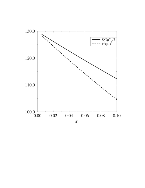
Figure 5: The free energy $\tilde{F}_{\mu}$ and the charge $\tilde{Q}$ as a function of the scaled chemical potential $\tilde{\mu}$ (denoted by $F^{\prime},Q^{\prime},\mu^{\prime}$ in this figure) for the Q-ball solution, in the limit of high temperatures and a small chemical potential. The extrapolated constant at $\tilde{\mu}\to 0$ is $C\approx 129.87(1)$, in accordance with the analytic result $C=4\pi^{4}/3$. The slopes are such that $\tilde{F}_{\mu}=C\tilde{\mu}^{-3}(1-2.1\tilde{\mu})$, $\tilde{Q}=3C\tilde{\mu}^{-4}(1-1.4\tilde{\mu})$.

Finally, note that in contrast to the leading terms, the first corrections to the asymptotic behaviour in eqs. (B.7), (B.8) depend on the detailed form of the potential $g(\tilde{\chi})$. As an example, consider the model in Sec. 4. With $a_{V}=(\pi^{2}/24)T^{4}$ and choosing $\tilde{\chi}=M_{\chi}/T=f\chi_{1}/(\sqrt{2}T)\equiv a_{\chi}^{-1}\chi_{1}$, we get

$$g(\tilde{\chi})=1+\frac{48}{\pi^{4}}J_{0}(\tilde{\chi})-\frac{3}{\pi^{4}}J_{0}(2\tilde{\chi}).$$ (B.9)

Here $J_{0}$ is from eq. (A.26). The numerical values following from the solution of eq. (B.2) with this $g(\tilde{\chi})$ are shown in Fig. 5. Since $\tilde{\mu}=(a_{\chi}/\sqrt{a_{V}})\mu=(4\sqrt{3}/f\pi)(\mu/T)$, it is seen from Fig. 5 that the asymptotic estimates in eqs. (B.7), (B.8) are reliable within $\sim 10$% at least up to $\tilde{\mu}\mathop{\raise 1.29167pt\hbox{$<$\kern-7.5pt\raise-4.73611pt\hbox{$\sim$}}}0.05$, or $\mu/T\mathop{\raise 1.29167pt\hbox{$<$\kern-7.5pt\raise-4.73611pt\hbox{$\sim$}}}0.02f$. This corresponds to charges $Q\mathop{\raise 1.29167pt\hbox{$>$\kern-7.5pt\raise-4.73611pt\hbox{$\sim$}}}10^{9}f^{-4}$.

References

• [1] R. Friedberg, T.D. Lee and A. Sirlin, Phys. Rev. D 13 (1976) 2739.
• [2] G. Rosen, J. Math. Phys. 9 (1968) 996; ibid. 9 (1968) 999.
• [3] S. Coleman, Nucl. Phys. B 262 (1985) 263.
• [4] F. Buccella, J.P. Derendinger, S. Ferrara and C.A. Savoy, Phys. Lett. B 115 (1982) 375; I. Affleck, M. Dine and N. Seiberg, Nucl. Phys. B 241 (1984) 493; Nucl. Phys. B 256 (1985) 557; M.A. Luty and W. Taylor, Phys. Rev. D 53 (1996) 3399; M. Dine, L. Randall and S. Thomas, Nucl. Phys. B 458 (1996) 291; T. Gherghetta, C. Kolda and S.P. Martin, Nucl. Phys. B 468 (1996) 37.
• [5] S. Dimopoulos, M. Dine, S. Raby, S. Thomas and J.D. Wells, Nucl. Phys. A (Proc. Suppl.) 52 (1997) 38; G.F. Giudice and R. Rattazzi, CERN-TH-97-380 [hep-ph/9801271]; and references therein.
• [6] G. Dvali, Q. Shafi and R. Schaefer, Phys. Rev. Lett. 73 (1994) 1886; G. Dvali, Phys. Lett. B 387 (1996) 471.
• [7] A. de Gouvêa, T. Moroi and H. Murayama, Phys. Rev. D 56 (1997) 1281.
• [8] A. Kusenko and M. Shaposhnikov, Phys. Lett. B 418 (1998) 46 [hep-ph/9709492].
• [9] A. Kusenko, Phys. Lett. B 405 (1997) 108 [hep-ph/9704273].
• [10] A. Kusenko, Phys. Lett. B 404 (1997) 285 [hep-th/9704073].
• [11] G. Dvali, A. Kusenko and M. Shaposhnikov, Phys. Lett. B 417 (1998) 99 [hep-ph/9707423].
• [12] I. Affleck and M. Dine, Nucl. Phys. B 249 (1985) 361.
• [13] A. Kusenko, V. Kuzmin, M. Shaposhnikov and P.G. Tinyakov, CERN-TH-97-346 [hep-ph/9712212].
• [14] A. Cohen, S. Coleman, H. Georgi and A. Manohar, Nucl. Phys. B 272 (1986) 301.
• [15] A.M. Safian, S. Coleman and M. Axenides, Nucl. Phys. B 297 (1988) 498.
• [16] T.D. Lee and Y. Pang, Phys. Rept. 221 (1992) 251, and references therein.
• [17] J.A. Frieman, G.B. Gelmini, M. Gleiser and E.W. Kolb, Phys. Rev. Lett. 60 (1988) 2101; K. Griest, E.W. Kolb and A. Massarotti, Phys. Rev. D 40 (1989) 3529.
• [18] J. Ellis, K. Enqvist, D.V. Nanopoulos and K.A. Olive, Phys. Lett. B 225 (1989) 313.
• [19] K. Griest and E.W. Kolb, Phys. Rev. D 40 (1989) 3231.
• [20] J.A. Frieman, A.V. Olinto, M. Gleiser and C. Alcock, Phys. Rev. D 40 (1989) 3241.
• [21] K.M. Benson and L.M. Widrow, Nucl. Phys. B 353 (1991) 187.
• [22] M. Axenides, Int. J. Mod. Phys. A 7 (1992) 7169.
• [23] A. Kusenko, Phys. Lett. B 406 (1997) 26 [hep-ph/9705361].
• [24] K. Enqvist and J. McDonald, hep-ph/9711514.
• [25] K. Enqvist and J. McDonald, hep-ph/9803380.
• [26] J.I. Kapusta, Finite-temperature Field Theory (Cambridge University Press, 1989).
• [27] A. Kusenko, M. Shaposhnikov and P.G. Tinyakov, JETP Lett. 67 (1998) 229 [hep-th/9801041].
• [28] A.D. Linde, Phys. Rev. D 14 (1976) 3345.
• [29] J.I. Kapusta, Phys. Rev. D 24 (1981) 426; H.E. Haber and H.A. Weldon, Phys. Rev. Lett. 46 (1981) 1497; Phys. Rev. D 25 (1982) 502.
• [30] J. Bernstein and S. Dodelson, Phys. Rev. Lett. 66 (1991) 683; K.M. Benson, J. Bernstein and S. Dodelson, Phys. Rev. D 44 (1991) 2480.
• [31] K. Farakos, K. Kajantie, K. Rummukainen and M. Shaposhnikov, Nucl. Phys. B 425 (1994) 67 [hep-ph/9404201]; K. Kajantie, M. Laine, K. Rummukainen and M. Shaposhnikov, Nucl. Phys. B 458 (1996) 90 [hep-ph/9508379].
• [32] A. Jakovác, K. Kajantie and A. Patkós, Phys. Rev. D 49 (1994) 6810; A. Jakovác and A. Patkós, Nucl. Phys. B 494 (1997) 54.
• [33] E. Braaten and A. Nieto, Phys. Rev. D 51 (1995) 6990; Phys. Rev. D 53 (1996) 3421.
• [34] M.E. Shaposhnikov, in Proceedings of the Summer School on Effective Theories and Fundamental Interactions, Erice, 1996, p. 360 [hep-ph/9610247].
• [35] D. Bödeker, W. Buchmüller, Z. Fodor and T. Helbig, Nucl. Phys. B 423 (1994) 171; J. Kripfganz, A. Laser and M.G. Schmidt, Z. Phys. C 73 (1997) 353.
• [36] K. Lee, Phys. Rev. D 50 (1994) 5333.
• [37] I.A. Belolaptikov et al, astro-ph/9802223.
• [38] A. Kusenko, M. Shaposhnikov, P.G. Tinyakov and I.I. Tkachev, Phys. Lett. B 423 (1998) 104 [hep-ph/9801212].
• [39] R. Schaeffer, Astron. Astrophys. 157 (1985) 13; R. Schaeffer, P. Delbourgo-Salvador and J. Audouze, Nature 317 (1985) 407.
• [40] H.E. Haber and G.L. Kane, Phys. Rep. 117 (1985) 75.