Bremsstrahlung and photon production
in thermal QCD

In this paper, we extend the study of bremsstrahlung photon production in a quark-gluon plasma to the cases of soft static photons $({\tenimbf q}={\tenimbf 0})$ and hard real photons. The general framework of this study is the effective perturbative expansion based on the resummation of hard thermal loops. Despite the fact that bremsstrahlung only comes at two loops, we find that in both cases it generates contributions of the same order of magnitude as those already calculated by several other groups at one loop. Furthermore, a new process contained in the two-loop diagrams dominate the emission of a very hard real photon. In all cases, the rate of real or virtual photon production in the plasma is appreciably increased compared to the one-loop predictions.

LAPTH–678/98, WIN–98-05, hep-ph/9804224

1 Introduction

We consider the production of a real photon or of a lepton pair in a quark-gluon plasma. The plasma is assumed to be in equilibrium at temperature $T$. The theoretical framework used in the calculation is that of thermal field theory improved by the hard loop resummation [1, 2, 3, 4, 5, 6] of Braaten and Pisarski: in this approach one distinguishes hard momenta, of order $T$, from soft momenta, of order $gT$, where $g$ is the Quantum Chromodynamics (QCD) coupling constant assumed to be small ($g\ll 1$). After resummation of hard thermal loops, one is led to an effective field theory from which observables can be evaluated perturbatively.

The production rates of real or virtual photons have already been evaluated, at the one loop level, in the effective theory [7, 8, 9, 10, 11]. Concerning soft virtual photons, it was found that the rate of production is considerably modified and enhanced compared to the result of the bare theory. Besides the usual quark-antiquark annihilation process, there appear many production mechanisms, in particular processes where the photon is radiated off a (hard) quark in a scattering process where the quark is backward scattered in the plasma via soft quark exchange. This is to be contrasted to the result obtained in a semi-classical approximation [12, 13, 14, 15, 16] where the photon is radiated off fast quarks in scattering processes mediated by a gluon exchange: we call such processes bremsstrahlung emission of a photon. In this study we reconcile the two approaches and show that the bremsstrahlung processes favored by the semi-classical approximation appear at the two-loop level in the effective theory and that, in fact, they contribute at the same order in $gT$ as the processes in the one-loop effective theory. Such a result should not be a surprise.

Consider the case of a soft virtual photon. The rate of production is related to the imaginary part of the vacuum polarization diagram [17, 18]. In the one-loop approximation of the effective field theory, it involves only effective fermion propagators and effective vertices [7]. A dominant contribution to the rate arises when the internal fermion momentum is soft and, therefore, all effective propagators and effective vertices have the same order of magnitude as their bare counterparts. A close examination of the final result shows, however, that it has a logarithmic sensitivity to scales of order $T$ (see section 3.3.2): this means that such a diagram also receives a dominant contribution from hard fermion momenta. When the momentum becomes large, the hard thermal loop (HTL) corrections to propagators and vertices are suppressed by, at least, a factor $g$ with respect to their bare counterparts. This suppression factor $g$ can easily be compensated by the larger phase space available to a hard fermion (${\cal O}(T)$) compared to soft fermion (${\cal O}(gT)$), thereby leading to a contribution of the same order of magnitude from the soft region and the hard region of phase-space. Now, when an observable is sensitive to the thermal corrections of hard vertices and propagators, it is obvious that all such corrections should be taken into account for the calculation to be complete. Some of these thermal corrections are naturally included in the lowest order of the effective theory via the resummation of hard thermal loops. But, even if the HTL approximation is correct for soft external particles, it does not account for all thermal corrections to hard vertices and hard propagators. For instance, neglecting the external momenta as one does in the calculation of the hard thermal loops is no longer justified when these momenta are not soft. Besides, equally important may be the contribution arising from soft gluons in the loop giving the HTL when the external momenta are hard, due to the Bose enhancement of the soft gluon term. Within the effective theory, both types of additional thermal corrections to a hard propagator or vertex are taken into account by considering a one-loop correction to this propagator or vertex.

In the calculation of the virtual photon production rate in the effective theory, soft gluon exchange appears in two-loop diagrams. It will be seen that the bremsstrahlung production mechanism is precisely given by these diagrams when the exchanged gluon is space-like. The evaluation of these diagrams is discussed below. These contributions are clearly not included in the effective one-loop diagram. This is obvious when looking at the corresponding physical processes and it manifests itself in the result by the calculated rate being proportional to the square of the thermal gluon mass $m_{\rm g}$, in contrast to the one-loop result where only the thermal quark mass appears [7]. Another important contribution of the two-loop diagrams is associated with time-like gluon exchanges: physically this represents QCD Compton scattering and quark-antiquark annihilation to produce a gluon and a photon. To evaluate this properly requires care since the two-loop diagrams with a hard time-like gluon exchanged are already part of the one-loop diagram with effective propagators and vertices. Taking into account the contribution of the appropriate counterterms in the effective lagrangian will prevent double-counting and allow the correct evaluation of the soft, time-like, gluon contribution.

The case of soft real photon production follows essentially the same pattern, except for the crucial fact that, the external line in the vacuum polarization diagram being massless, collinear divergences appear when evaluating the two-loop diagrams: the quasi-overlap of two such divergences, associated with the fermion propagators, leads to an enhancement factor of ${\cal O}(1/g^{2})$ [19, 20]. The paradoxical result then follows that the one-loop contribution is relatively suppressed by a factor $g^{2}$ compared to the two-loop one! The latter is entirely dominated by the bremsstrahlung process since the kinematical constraints require the gluon to be space like for the enhancement factor to occur. The Compton and annihilation mechanisms are sub-dominant.

The case of a hard real photon, of momentum of ${\cal O}(T)$, shares features with both cases above. The one-loop approximation has a logarithmic sensitivity to the hard fermion momentum in the loop [10, 11]. The two-loop bremsstrahlung has a $1/g^{2}$ collinear enhancement, as in the real soft photon case, which however is compensated by a factor $m_{\rm g}^{2}/q^{2}\sim g^{2}$, where $q$ is the photon momentum, leaving the bremsstrahlung contribution at the same order in $gT$ as the one-loop contribution.

In the following we are concerned mainly with the bremsstrahlung part of the two-loop diagrams, and leave the discussion of the Compton and annihilation processes and their interplay with the counterterms of the effective theory to future work. We do not discuss the production of soft real photons since this has already been studied in detail in [19].

In the next section we derive the general expression for the (real or virtual) photon production rate at the two loop level. Then we consider the case of soft virtual photons produced at rest in the plasma and derive the leading behavior analytically. We compare to the one-loop results and show that the bremsstrahlung contribution is numerically dominant although both contributions are technically of the same order in $g$. The semi-classical approach is then discussed and it is shown that even though the approximations inherent in the semi-classical approach are not really justified in the case of soft photon production in a quark-gluon plasma, it leads to a result quite comparable to that obtained in thermal field theory. Turning to the case of hard real photons, it is shown that the bremsstrahlung mechanism is of the same order as the already calculated one-loop result. Carrying out a more detailed comparison with the latter approach, it is found that the bremsstrahlung process dominates over the one-loop result for photon momentum of ${\cal O}(T)$ but is relatively suppressed by a logarithmic factor for hard enough photons. For very hard energies, we find that the photon production is in fact dominated by a new process consisting of a $q\bar{q}$ annihilation where the quark or antiquark undergoes a scattering in the medium. We summarize all the thermal field theory results concerning real and virtual photon production in a concluding section.

The role of counterterms in the application of the effective theory up to two-loops is discussed in a first appendix where the problem is also illustrated in a simple example. In a second appendix, the importance of phase space factors in thermal calculations is emphasized and the difference with the zero temperature phase space is made clear.

2 Bremsstrahlung in thermal field theory

2.1 Topologies involving bremsstrahlung

Let us first recall the relationship between the photon production rate and the imaginary part of the retarded polarization tensor of the photon, as given by thermal field theory (we follow the notations of [21]). For real photons, this relation gives the number of photon emitted per unit time and per unit volume of the plasma as [17, 18]:

$${{dN}\over{dtd{\tenimbf x}}}=-{{d{\tenimbf q}}\over{(2\pi)^{3}2q_{o}}}\;2n_{{}_{B}}(q_{o})\,{\rm Im}\,\Pi^{{}^{RA}}{}_{\mu}{}^{\mu}(q_{o},{\tenimbf q})\;,$$ (1)

whereas for the production of a photon of invariant mass $Q^{2}$ decaying into a lepton pair we have:

$${{dN}\over{dtd{\tenimbf x}}}=-{{dq_{o}d{\tenimbf q}}\over{12\pi^{4}}}\;{\alpha\over{Q^{2}}}\,n_{{}_{B}}(q_{o})\,{\rm Im}\,\Pi^{{}^{RA}}{}_{\mu}{}^{\mu}(q_{o},{\tenimbf q})\;.$$ (2)

Basically, the above two formulae differ only by the allowed phase space for the photon, by an extra QED coupling constant when the photon decays into a lepton pair, and by the propagator of a heavy photon. It is worth recalling that these relations are valid only at first order in the QED coupling $\alpha$ since they do not take into account the possible re-interactions of the photon on its way out of the plasma nor the simultaneous emission of more than one photon. Nevertheless, they are true to all orders in the strong coupling constant $\alpha_{{}_{S}}$. This should not be a serious limitation from a practical point of view since $\alpha\ll\alpha_{{}_{S}}$.

Let us now examine in which topologies the bremsstrahlung can appear. It is worth recalling at this point that the retarded imaginary part in Eqs. (1) and (2) can be expressed as a sum over possible cuts through the diagram [22, 23, 24]. Therefore, we need to look for diagrams that will give bremsstrahlung processes once cut. A simple inspection of the processes involved in one-loop contributions (see [7, 19] for instance) shows that bremsstrahlung does not appear at this order. To see bremsstrahlung processes, one should consider the two-loop contributions of Fig. 1.

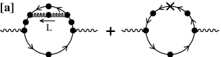
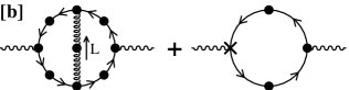
Figure 1: Two-loop contributions involving bremsstrahlung processes. A black dot denotes an effective propagator or vertex. Crosses are HTL counterterms.

The diagrams have been obtained via a strict application of the Feynman rules of the effective theory [3, 5], giving a priori effective vertices and propagators and diagrams with counterterms in order to avoid any double counting of thermal corrections already included at the one-loop level via the resummation of hard thermal loops, as outlined in appendix A. To make the connection with previous works [19, 20] easier, we mention that looking at two loop diagrams in the effective theory is just a more rigorous way of doing what we might call “calculating one-loop diagrams beyond the HTL approximation”. Our present formulation is indeed more rigorous since it takes care of the counterterms, and also more positive since it does not assume a priori that one needs to go beyond the effective theory. Among all the possible cuts through the diagrams, those that correspond to bremsstrahlung necessarily cut the gluon propagator. Moreover, if $L$ is the gluon 4-momentum, only the Landau damping part $(L^{2}<0)$ gives bremsstrahlung, the $L^{2}>0$ part rather giving Compton effect or $q\bar{q}$-like annihilations [25]. There is another reason why the region $L^{2}>0$ deserves a separate treatment: in the $L^{2}<0$ kinematical domain, it is obvious that we cannot have contributions coming from the HTL counterterms since these counterterms involve only bare gluon propagators that don’t have any imaginary part in the space-like region. On the contrary, in the $L^{2}>0$ region, one should pay special attention to the counterterm diagrams in order to avoid any double-counting. Indeed, when the gluon becomes hard, we have a hard loop that may reproduce what is already included in the one-loop diagram via the effective vertices and propagators. From now on, we limit ourselves to the region where $L^{2}<0$ and only to the true two-loop diagrams, leaving the $L^{2}>0$ region and the discussion of counterterms to future work.

Moreover, since our main focus is on bremsstrahlung, we must retain from the cut quark propagators only the pole part and reject the Landau damping part, which would correspond to a different physical process. For the same reason, the cut should avoid going through an effective vertex.

2.2 General expression of two-loop contributions

In order to obtain a bremsstrahlung contribution of the same order of magnitude as the already calculated one-loop contributions, we need a hard phase space for the quark circulating in the loop, as explained in appendix B. We will see later that we have such contributions in the diagrams depicted in Fig. 1. Therefore, at leading order, we can use “bare” vertices and propagators everywhere except for the gluon propagator since the gluon can be soft. The diagrams we have to consider are therefore the simplified versions of the previous ones represented on Fig. 2.

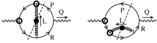
Figure 2: Simplified two-loop contributions involving bremsstrahlung processes. The circled vertices correspond to the framework of the cutting rules.

In the same figure, we have depicted the relevant cuts as well as the arrangement of circlings that enables one to calculate the corresponding contribution in the framework of the thermal cutting rules. We have checked that the two cuts represented form a gauge independent set of terms, to which one should add the symmetric cut for the vertex diagram and a third diagram with the self-energy correction on the upper quark line. Since these two other terms give the same contribution as the previous two, we simply take them into account by multiplying the final result by an overall factor of 2.

A straightforward application of the cutting rules valid for the “R/A” formalism, with the notations of [24], gives for the vertex correction:

$$\halign to=0.0pt{\@eqnsel\hskip\@centering$\displaystyle{#}$&\global\@eqcnt\@ne\hskip 2\arraycolsep\hfil${#}$\hfil&\global\@eqcnt\tw@\hskip 2\arraycolsep$\displaystyle{#}$\hfil&\llap{#}\cr 0.0pt plus 1000.0pt$\displaystyle{&10.0pt\hfil${&10.0pt$\displaystyle{\!\!\! {\rm Im}\,\Pi^{{}^{RA}} {}_{\mu}{}^{\mu}(q_{o},{\tenimbf q})_{|_{\rm vertex}}\!\!\!=- {\rm Im}\,\Pi^{{}^{AR}} {}_{\mu}{}^{\mu}(q_{o},{\tenimbf q})_{|_{\rm vertex}}= {{NC_{{}_{F}}}\over 2} \int{{d^{4}P}\over{(2\pi)^{4}}}\int{{d^{4}L}\over{(2\pi)^{4}}} \\ &\hbox to0.0pt{\hss&\times\;e^{{}^{\underline{ARR}}}(Q,P+L,-R-L)g^{{}^{\underline{ARR}}}(-P-L,P,L)\\&&\times\;g^{{}^{{AAR}}}(R+L,-L,-R)e^{{}^{{AAR}}}(R,-P,-Q)\\&&\times\;{\rm Tr}\,\left[\gamma^{\mu}{\cal S}^{{}^{\underline{AR}}}(P+L)\gamma^{\rho}{\cal S}^{{}^{A\underline{R}}}(P)\gamma_{\mu}\right.\left.{\cal S}^{{}^{RA}}(R)\gamma^{\sigma}{\cal S}^{{}^{\underline{R}A}}(R+L)\right]D^{{}^{A\underline{R}}}_{\rho\sigma}(L)\\&&=-{{NC_{{}_{F}}}\over 2}e^{2}g^{2}\int{{d^{4}P}\over{(2\pi)^{4}}}\!\!\!\int{{d^{4}L}\over{(2\pi)^{4}}}\left[\Delta^{{}^{R}}_{{}_{T,L}}(L)\!-\!\Delta^{{}^{A}}_{{}_{T,L}}(L)\right]\\&&\times\;\left[S^{{}^{R}}(P)-S^{{}^{A}}(P)\right]\left[S^{{}^{R}}(R+L)-S^{{}^{A}}(R+L)\right]\\&&\times\;\left(n_{{}_{F}}(r_{o})-n_{{}_{F}}(p_{o})\right)\left(n_{{}_{B}}(l_{o})+n_{{}_{F}}(r_{o}+l_{o})\right)\\&&\times\;S(R)S(P+L)P_{\rho\sigma}^{{}^{T,L}}(L)\;{\rm Trace}^{\rho\sigma}{}_{|_{\rm vertex}}\;,&(3)\cr}}}}}$$

where, following [19], we denote the fermion propagator:

$${\cal S}^{{}^{R,A}}(P)\equiv{\overline{\raise 0.6458pt\hbox{$/$}\kern-5.29999pt\hbox{$P$}}}S^{{}^{R,A}}(P){\ \rm with\ }{\overline{P}}\equiv(p_{o},\sqrt{p^{2}+M^{2}_{\infty}}\,\hat{\tenimbf p})$$ (4)

$$S(P)^{{}^{R,A}}\equiv{i\over{{\overline{P}}^{2}\pm ip_{o}\varepsilon}}={i\over{P^{2}-M^{2}_{\infty}\pm ip_{o}\varepsilon}}\;,$$ (5)

and the effective gluon propagator in a linear covariant gauge:

$$-D_{\rho\sigma}^{{}^{R,A}}(L)\equiv P^{{}^{T}}_{\rho\sigma}(L)\Delta^{{}^{R,A}}_{{}_{T}}(L)+P^{{}^{L}}_{\rho\sigma}(L)\Delta^{{}^{R,A}}_{{}_{L}}(L)+\xi L_{\rho}L_{\sigma}/L^{2}$$ (6)

$$\Delta^{{}^{R,A}}_{{}_{T,L}}(L)\equiv\left.{i\over{L^{2}-\Pi_{{}_{T,L}}(L)}}\right|_{{}_{R,A}}{\ \rm and\ \ }\rho_{{}_{T,L}}(L)\equiv{\rm Disc}\Delta^{{}^{R}}_{{}_{T,L}}(L)$$ (7)

$$\Pi_{{}_{T}}(L)\equiv 3m_{\rm g}^{2}\left[{{x^{2}}\over 2}+{{x(1-x^{2})}\over{4}}\ln\left({{x+1}\over{x-1}}\right)\right]$$ (8)

$$\Pi_{{}_{L}}(L)\equiv 3m_{\rm g}^{2}(1-x^{2})\left[1-{{x}\over{2}}\ln\left({{x+1}\over{x-1}}\right)\right]\;,$$ (9)

with $P^{{}^{T,L}}_{\rho\sigma}$ the usual transverse and longitudinal projectors in linear covariant gauges [2, 27, 28, 29, 30], $M^{2}_{\infty}\equiv g^{2}C_{{}_{F}}T^{2}/4$ [26] the asymptotic thermal mass of the quark, and $m_{\rm g}^{2}\equiv g^{2}T^{2}[N+N_{{}_{F}}/2]/9$ the soft gluon thermal mass. In this formula, $e$ is the electric charge of the quark and therefore depends on its flavor. Likewise, we obtain for the second diagram:

$$\halign to=0.0pt{\@eqnsel\hskip\@centering$\displaystyle{#}$&\global\@eqcnt\@ne\hskip 2\arraycolsep\hfil${#}$\hfil&\global\@eqcnt\tw@\hskip 2\arraycolsep$\displaystyle{#}$\hfil&\llap{#}\cr 0.0pt plus 1000.0pt$\displaystyle{&10.0pt\hfil${&10.0pt$\displaystyle{\!\!\!{\rm Im}\,\Pi^{{}^{RA}} {}_{\mu}{}^{\mu}(q_{o},{\tenimbf q})_{|_{\rm self}}=- {\rm Im}\,\Pi^{{}^{AR}} {}_{\mu}{}^{\mu}(q_{o},{\tenimbf q})_{|_{\rm self}}= {{NC_{{}_{F}}}\over 2} \int{{d^{4}P}\over{(2\pi)^{4}}}\int{{d^{4}L}\over{(2\pi)^{4}}} \\ &\hbox to0.0pt{\hss&\times\;e^{{}^{\underline{ARR}}}(Q,P,-R)g^{{}^{\underline{ARR}}}(R,L,-R-L)\\&&\times\;g^{{}^{{AAR}}}(R+L,-L,-R)e^{{}^{{AAR}}}(R,-P,-Q)\\&&\times\;{\rm Tr}\,\left[\gamma^{\mu}{\cal S}^{{}^{A\underline{R}}}(P)\gamma_{\mu}{\cal S}^{{}^{{RA}}}(R)\gamma^{\rho}\right.\left.{\cal S}^{{}^{\underline{R}A}}(R+L)\gamma^{\sigma}{\cal S}^{{}^{\underline{RA}}}(R)\right]D^{{}^{A\underline{R}}}_{\rho\sigma}(L)\\&&=-{{NC_{{}_{F}}}\over 2}e^{2}g^{2}\int{{d^{4}P}\over{(2\pi)^{4}}}\int{{d^{4}L}\over{(2\pi)^{4}}}\left[\Delta^{{}^{R}}_{{}_{T,L}}(L)-\Delta^{{}^{A}}_{{}_{T,L}}(L)\right]\\&&\times\;\left[S^{{}^{R}}(P)-S^{{}^{A}}(P)\right]\left[S^{{}^{R}}(R+L)-S^{{}^{A}}(R+L)\right]P_{\rho\sigma}^{{}^{T,L}}(L)\;{\rm Trace}^{\rho\sigma}{}_{|_{\rm self}}\\&&\times\;\left(S(R)\right)^{2}\left(n_{{}_{F}}(r_{o})-n_{{}_{F}}(p_{o})\right)\left(n_{{}_{B}}(l_{o})+n_{{}_{F}}(r_{o}+l_{o})\right)\;.&(10)\cr}}}}}$$

In the previous formulae, a factor $S(R)$ without any $R$ or $A$ superscript simply denotes the principal part of the propagator. In other words, for these factors, the $R$ or $A$ prescription is irrelevant because the corresponding delta function is incompatible with the other delta functions present and therefore vanishes.

We may notice the similarity between Eqs. (2.2) and (2.2). In particular, the same combination of statistical weights appear in both formulae, while the expressions in the square brackets simply express the cuts on internal lines. Moreover, when plugged into Eq. (1) in order to obtain the production rate, the sum of Eqs. (2.2) and (2.2) gives the more intuitive Eq. (B) in appendix B (to which one should add similar terms to take into account all the processes included in our diagrams). Therefore, the “R/A” formalism appears just as an efficient method to reorder the factors of the integrand in order to make it more compact and more convenient for the subsequent integrations. The drawback of this formalism is that it generates less intuitive expressions.

2.3 Common part of the calculation

The calculation of the Dirac’s traces is of course common to both cases. We obtain for the self-energy insertion:

$$\halign to=0.0pt{\@eqnsel\hskip\@centering$\displaystyle{#}$&\global\@eqcnt\@ne\hskip 2\arraycolsep\hfil${#}$\hfil&\global\@eqcnt\tw@\hskip 2\arraycolsep$\displaystyle{#}$\hfil&\llap{#}\cr 0.0pt plus 1000.0pt$\displaystyle{&10.0pt\hfil${&10.0pt$\displaystyle{{\rm Trace}{}^{\rho\sigma}{}_{|_{\rm self}} \approx-4\left[ 4{\overline{R}}{}^{2}Q{}^{\rho}{\overline{R}}{}^{\sigma}-4Q{}^{2}{\overline{R}}{}^{\rho}{\overline{R}}{}^{\sigma}\right. \\ &\hbox to0.0pt{\hss&\qquad\qquad\left.-g{}^{\rho\sigma}\left({\overline{R}}{}^{2}({\overline{R}}{}^{2}-Q{}^{2})+2{\overline{R}}{}^{2}Q\cdot L-2Q{}^{2}{\overline{R}}\cdot L\right)\right]\;,&(11)\cr}}}}}$$

and for the vertex correction:

$$\halign to=0.0pt{\@eqnsel\hskip\@centering$\displaystyle{#}$&\global\@eqcnt\@ne\hskip 2\arraycolsep\hfil${#}$\hfil&\global\@eqcnt\tw@\hskip 2\arraycolsep$\displaystyle{#}$\hfil&\llap{#}\cr 0.0pt plus 1000.0pt$\displaystyle{&10.0pt\hfil${&10.0pt$\displaystyle{{\rm Trace}{}^{\rho\sigma}{}_{|_{\rm vertex}} \approx-4\left[2{\overline{R}}{}^{2}{\overline{P}}{}^{\rho}Q{}^{\sigma}-2({\overline{P+L}}){}^{2}{\overline{R}}{}^{\rho}Q{}^{\sigma}\right. \\ &\hbox to0.0pt{\hss&\qquad+2L{}^{2}({\overline{R}}{}^{\rho}{\overline{R}}{}^{\sigma}+{\overline{P}}{}^{\rho}{\overline{P}}{}^{\sigma})-4Q{}^{2}{\overline{R}}{}^{\rho}{\overline{P}}{}^{\sigma}\\&&\qquad+g{}^{\rho\sigma}\left(\left.-L{}^{2}({\overline{R}}{}^{2}+({\overline{P+L}}){}^{2}-Q{}^{2}-L{}^{2})\right)\right]\;.&(12)\cr}}}}}$$

It is worth recalling that these expressions are obtained by anticipating the use of the relation

$$L^{\rho}P^{{}^{T,L}}_{\rho\sigma}(L)=0$$ (13)

in order to drop any $L^{\rho}$ or $L^{\sigma}$ in the expression of the Dirac’s traces. Since this identity is not true for the gauge dependent part of the gluon propagator, one should not use these expressions of the traces to check the independence of the rate with respect to the gauge parameter $\xi$. Moreover, we discarded terms that will be killed later by the delta functions such as the one contained in $S^{{}^{R}}(P)-S^{{}^{A}}(P)=2\pi\epsilon(p_{o})\delta(P^{2}-M^{2}_{\infty})$. Since a 4-vector like ${\overline{P}}=(p_{o},\sqrt{p^{2}+M^{2}_{\infty}}\,\hat{\tenimbf p})$ is not a linear function of the momentum $P$, we used some approximations to simplify the calculations, the effect of which is to neglect only terms that are always subdominant.

We also notice that the statistical weights and delta functions present in Eqs. (2.2) and (2.2) are invariant under the change of variables $P\to-R-L$, $L\to L$. Therefore, in the remaining factors of the integrand, we are allowed to drop the parts which are antisymmetric under this transformation. Collecting contributions from the two topologies, this symmetrization gives:

$$\halign to=0.0pt{\@eqnsel\hskip\@centering$\displaystyle{#}$&\global\@eqcnt\@ne\hskip 2\arraycolsep\hfil${#}$\hfil&\global\@eqcnt\tw@\hskip 2\arraycolsep$\displaystyle{#}$\hfil&\llap{#}\cr 0.0pt plus 1000.0pt$\displaystyle{&10.0pt\hfil${&10.0pt$\displaystyle{\left[{{{\rm Trace}{}^{\rho\sigma}{}_{|_{\rm vertex}}} \over{\overline{R}{}^{2}(\overline{P+L}){}^{2}}} +{{{\rm Trace}{}^{\rho\sigma}{}_{|_{\rm self}}} \over{\overline{R}{}^{2}\overline{R}{}^{2}}}\right]_{\rm sym}\approx-4\left[ 2L{}^{2}{{\overline{R}{}^{\rho}\overline{R}{}^{\sigma}+ \overline{P}{}^{\rho}\overline{P}{}^{\sigma}} \over{\overline{R}{}^{2}(\overline{P+L}){}^{2}}} \right.\\ &\hbox to0.0pt{\hss&\qquad-2{Q{}^{2}}\left({{\overline{R}{}^{\rho}}\over{\overline{R}{}^{2}}}+{{\overline{P}{}^{\rho}}\over{(\overline{P+L}){}^{2}}}\right)\left({{\overline{R}{}^{\sigma}}\over{\overline{R}{}^{2}}}+{{\overline{P}{}^{\sigma}}\over{(\overline{P+L}){}^{2}}}\right)\\&&\qquad-g{}^{\rho\sigma}\left(1-{{L{}^{2}(L{}^{2}+Q{}^{2})}\over{\overline{R}{}^{2}(\overline{P+L}){}^{2}}}+({{L^{2}+Q\cdot L}})\left({1\over{\overline{R}{}^{2}}}+{1\over{(\overline{P+L}){}^{2}}}\right)\right.\\&&\qquad\left.\left.+{{Q{}^{2}L{}^{2}}\over{2}}\left({{1}\over{(\overline{R}{}^{2})^{2}}}+{{1}\over{((\overline{P+L}){}^{2})^{2}}}\right)\right)\right]\;,&(15)\cr}}}}}$$

which will be our starting point in the following sections.

3 Contribution to soft static photons

3.1 Kinematics

When the 3-momentum ${\tenimbf q}$ of the emitted photon is zero, a lot of simplifications occur. First of all, since there is one 3-vector less in the problem, we need only one angular variable which simplifies considerably the angular integrations. Moreover, as shown in [19], the non vanishing invariant mass of the emitted photon regulates all the potential collinear divergences when $Q^{2}/q_{o}^{2}\sim 1$. Therefore, one can simply forget about the quark asymptotic thermal mass since the purpose of such a mass is precisely to regularize collinear singularities. This means that we can everywhere identify $P$ and $\overline{P}$ at this level of approximation, since furthermore $P$ is hard.

From the identity $S^{{}^{R}}(P)-S^{{}^{A}}(P)=2\pi\epsilon(p_{o})\delta(P^{2})$, we extract the values $p_{o}=\pm p$ and $r_{o}=q_{o}\pm p$. For the second cut quark propagator, we have the identity $S^{{}^{R}}(R+L)-S^{{}^{A}}(R+L)=2\pi\epsilon(r_{o}+l_{o})\delta((R+L)^{2})$ from which we extract the cosine of the angle $\theta^{\prime}$ between ${\tenimbf p}$ and ${\tenimbf l}$:

$$\cos\theta^{\prime}={{(r_{o}+l_{o})^{2}-p^{2}-l^{2}}\over{2pl}}\;.$$ (16)

Of course, we must require that this value be in $[-1,+1]$, which will reduce the available phase space.

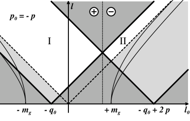
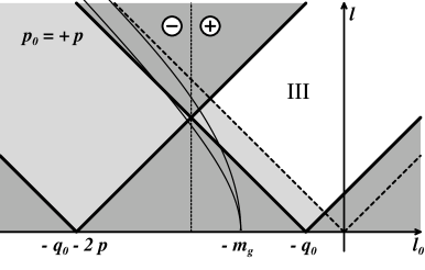
Figure 3: Allowed domains in the $(l_{o},l)$ plane for $p_{o}=\pm p$. The area shaded in dark gray is excluded by the delta functions. The region shaded in light gray is above the light–cone (dotted lines). The solid curves are the transverse and longitudinal dispersion curves of the thermalized gluon. The vertical dotted line is the separation between $\epsilon(p_{o})\epsilon(r_{o}+l_{o})=+1$ and $\epsilon(p_{o})\epsilon(r_{o}+l_{o})=-1$. The value of the thermal mass has been exaggerated in order to make the figure more readable.

This requirement leads to the following two inequalities:

$$(l_{o}-l+p_{o}+q_{o}-p)(l_{o}+l+p_{o}+q_{o}+p)\leq 0$$ (17)

$$(l_{o}-l+p_{o}+q_{o}+p)(l_{o}+l+p_{o}+q_{o}-p)\geq 0\;,$$ (18)

which lead to a phase space reduction that can be seen in Fig. 3, where the region excluded by the requirement $\cos\theta^{\prime}\in[-1,+1]$ has been shaded in dark gray. Other regions are excluded also by our choice of looking only at bremsstrahlung, i.e. excluding areas where $L^{2}>0$ [25]. Finally, the only regions we have to consider are the unshaded ones.

Having taken these constraints into account, the independent variables we are left with are for instance (the choice is not unique) $r=p$, $l_{o}$ and $l$, everything else being a function of these three. In particular, the denominators appearing in the calculations are

$$R^{2}=q_{o}(q_{o}\pm 2p)$$ (19)

$$(P+L)^{2}=-q_{o}(q_{o}+2l_{o}\pm 2p)\;,$$ (20)

the $+$ sign corresponding to $p_{o}=+p$ and the $-$ sign to $p_{o}=-p$.

It is worth examining more closely to which physical processes the regions I, II and III correspond. This is done just by looking at the signs of $p_{o}$ and $r_{o}+l_{o}$. Examples are shown in Fig. 4.

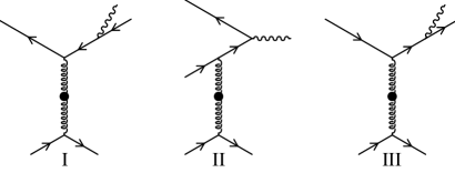
Figure 4: Physical processes included in the diagrams of Fig. 2, in the region $L^{2}<0$. Region I: $p_{o}<0$, $r_{o}+l_{o}<0$: bremsstrahlung with an antiquark. Region II: $p_{o}<0$, $r_{o}+l_{o}>0$: $q\bar{q}$ annihilation with scattering. Region III: $p_{o}>0$, $r_{o}+l_{o}>0$: bremsstrahlung with a quark. The particle on which the quark is scattered can also be a gluon.

Besides the bremsstrahlung present in regions I and III, we see a new process in region II. This process corresponds to an annihilation of a quark-antiquark pair, one of the particles having previously undergone a scattering in the medium. Since the scale for the quark momentum is given by the temperature $(p={\cal O}(T))$, and since we are looking here at soft photons, it is obvious from Fig. 3 that processes I and III have support of order $T^{2}$ in the $(l_{o},l)$ plane while process II has only support of order $q_{o}T$, the integrand being the same. Therefore, we expect and we have checked that process II is suppressed by a factor of order $q_{o}/T\ll 1$ compared to bremsstrahlung. As a consequence, bremsstrahlung appears to be the dominant contribution as far as the $L^{2}<0$ domain is concerned. In the remaining part of this section, we limit our study to the regions I and III. We can obtain a further reduction of the phase space by noticing that regions I and III give the same contribution since they are equivalent by a change of variables (indeed, after the symmetrization in Eq. (2.3), the integrands are invariant under the change of variables $P\to-R-L$ and $L\to L$). Physically, this means that photons are produced equally by quarks and by antiquarks. Therefore, we just consider region III (i.e. $p_{o}>0$ and $r_{o}+l_{o}>0$) and multiply the result by an extra factor $2$. Hence, the contribution of bremsstrahlung is given by

$$\halign to=0.0pt{\@eqnsel\hskip\@centering$\displaystyle{#}$&\global\@eqcnt\@ne\hskip 2\arraycolsep\hfil${#}$\hfil&\global\@eqcnt\tw@\hskip 2\arraycolsep$\displaystyle{#}$\hfil&\llap{#}\cr 0.0pt plus 1000.0pt$\displaystyle{&10.0pt\hfil${&10.0pt$\displaystyle{{\rm Im}\,\Pi^{{}^{AR}}{}_{\mu}{}^{\mu}(q_{o},{\tenimbf 0})\approx{{NC_{{}_{F}}}\over{(2\pi)^{4}}} e^{2}g^{2}\int dp\int ldl \int dl_{o} \\ &\hbox to0.0pt{\hss&\qquad\times\;\left[n_{{}_{F}}(r_{o})-n_{{}_{F}}(p_{o})\right]\left[n_{{}_{B}}(l_{o})+n_{{}_{F}}(r_{o}+l_{o})\right]\\&&\qquad\times\sum\limits_{a=T,L}\rho_{a}(L)P^{a}_{\rho\sigma}(L)\left[{{{\rm Trace}{}^{\rho\sigma}{}_{|_{\rm vertex}}}\over{\overline{R}{}^{2}(\overline{P+L}){}^{2}}}+{{{\rm Trace}{}^{\rho\sigma}{}_{|_{\rm self}}}\over{\overline{R}{}^{2}\overline{R}{}^{2}}}\right]_{{\rm sym\ \ \ \ }\atop{{p_{o}=p\ \ \ }\atop{\cos\theta^{\prime}}=\cdots}}\!\!\!.&(21)\cr}}}}}$$

3.2 Extraction of the dominant terms

3.2.1 General considerations

Let us now concentrate on the matrix element to be integrated over the phase space depicted above. In order to perform the contraction of the Dirac’s trace obtained in Eq. (2.3) with the longitudinal projectors, we use the following expressions [27, 28]

$$P^{{}^{T}}_{\rho\sigma}(L)=g_{\rho\sigma}-U_{\rho}U_{\sigma}+{{(L_{\rho}-l_{o}U_{\rho})(L_{\sigma}-l_{o}U_{\sigma})}\over{l^{2}}}$$ (22)

$$P^{{}^{L}}_{\rho\sigma}(L)=-P^{{}^{T}}_{\rho\sigma}(L)+g_{\rho\sigma}-{{L_{\rho}L_{\sigma}}\over{L^{2}}}\;,$$ (23)

where $U\equiv(1,{\tenimbf 0})$ is the 4-velocity of the plasma in its rest frame. An important simplification is obtained in the case of static photons since we have

$$Q^{\rho}P^{{}^{T}}_{\rho\sigma}=0\;.$$ (24)

Taking into account this simplification, we obtain after some algebra:

$$\halign to=0.0pt{\@eqnsel\hskip\@centering$\displaystyle{#}$&\global\@eqcnt\@ne\hskip 2\arraycolsep\hfil${#}$\hfil&\global\@eqcnt\tw@\hskip 2\arraycolsep$\displaystyle{#}$\hfil&\llap{#}\cr 0.0pt plus 1000.0pt$\displaystyle{&10.0pt\hfil${&10.0pt$\displaystyle{\sum\limits_{a=T,L}\rho_{a}(L) P^{a}_{\rho\sigma}(L) \left[{{{\rm Trace}{}^{\rho\sigma}{}_{|_{\rm vertex}}} \over{\overline{R}{}^{2}(\overline{P+L}){}^{2}}} +{{{\rm Trace}{}^{\rho\sigma}{}_{|_{\rm self}}} \over{\overline{R}{}^{2}\overline{R}{}^{2}}}\right]_{\rm sym} \approx\\ &\hbox to0.0pt{\hss&\qquad-4\left[\left(\rho_{{}_{T}}(L)-\rho_{{}_{L}}(L)\right){{4p^{2}(\cos^{2}\theta^{\prime}-1)}\over{R^{2}(P+L)^{2}}}\left(L^{2}-2{{Q^{2}(Q\cdot L)^{2}}\over{R^{2}(P+L)^{2}}}\right)\right.\\&&\qquad+2{{(Q+L)^{2}}\over{R^{2}(P+L)^{2}}}\left(Q^{2}\rho_{{}_{L}}(L)+L^{2}\rho_{{}_{T}}(L)\right)\\&&\qquad-2\rho_{{}_{T}}(L)\left(1-2{{(Q\cdot L)^{2}}\over{R^{2}(P+L)^{2}}}\right.\\&&\qquad\qquad\qquad\left.\left.+{{Q^{2}L^{2}}\over 2}\left[{1\over{(R^{2})^{2}}}+{1\over{((P+L)^{2})^{2}}}\right]\right)\right]\;.&(25)\cr}}}}}$$

It is worth noticing that all the potential poles in $1/L^{2}$ (see Eq. (23-b)) have disappeared in this formula. This is nothing but a consequence of the gauge invariance of the set of diagrams we are looking at.

Now, in order to extract the order of magnitude of each term in Eq. (3.2.1), we can use the following very rough rules:

$\bullet$ $R^{2}\sim(P+L)^{2}\sim 2pq_{o}$ which is correct for our purpose even if $l$ is hard since $l$ is bounded by a quantity proportional to $p$ (see the previous paragraph on kinematics).

$\bullet$ $n_{{}_{B}}(l_{o})\sim T/l_{o}$ which always gives the correct order of magnitude, even when $l_{o}$ is hard.

$\bullet$ $n_{{}_{F}}(r_{o}+l_{o})={\cal O}(1)$.

$\bullet$ $n_{{}_{F}}(r_{o})-n_{{}_{F}}(p_{o})\approx q_{o}n^{\prime}_{{}_{F}}(p)$.

$\bullet$ $1-\cos^{2}\theta^{\prime}={\cal O}(1)$.

$\bullet$ The details of the $x$ dependence are irrelevant to obtain the correct order of magnitude.

$\bullet$ $\rho_{{}_{T,L}}(l,x)$ behaves like $m_{\rm g}^{2}/(l^{2}+m_{\rm g}^{2})^{2}$ if one neglects its $x$ dependence.

Moreover, using the variable $x\equiv l_{o}/l$, we can see ${\rm Im}\,\Pi^{{}^{AR}}{}_{\mu}{}^{\mu}(q_{o},{\tenimbf 0})$ is a sum of terms like

$$e^{2}g^{2}q_{o}^{\alpha}\int dp\,n^{\prime}_{{}_{F}}(p)p^{\beta}\int dl\,l^{\gamma}\int dx\,F(x)\rho_{{}_{T,L}}(l,x)\left({{T}\over{l}}+{\cal O}(1)\right)\;,$$ (26)

where $F(x)$ is a dimensionless function and where $\alpha+\beta+\gamma=3$ in order to give the correct overall dimension. A close inspection of Eq. (3.2.1) shows that $\alpha$ ranges from $\alpha=-1$ to $\alpha=3$, taking all the integer values between these bounds. Eq. (3.2.1) shows also that $\beta\leq 0$. From the previous structure and since we can factorize a factor $m_{\rm g}^{2}$ out of the spectral functions $\rho_{{}_{T,L}}$, it is obvious that we can write the result as

$${\rm Im}\,\Pi^{{}^{AR}}{}_{\mu}{}^{\mu}(q_{o},{\tenimbf 0})\approx e^{2}g^{2}{{m^{2}_{\rm g}T}\over{q_{o}}}P\left({{q_{o}}\over{m_{\rm g}}},{{q_{o}}\over{T}}\right)\;,$$ (27)

where $P(\cdot)$ is a polynomial of two variables, of total degree $4$. Under the assumption that $q_{o}\ll T$, we are allowed to truncate this polynomial and keep only terms of degree $0$ in the variable $q_{o}/T$, leaving a polynomial of $q_{o}/m_{\rm g}$ only. Moreover, the above rules show that the term of Eq. (3.2.1) proportional to $p^{2}(\cos^{2}\theta^{\prime}-1)L^{2}$ contributes to the constant term of this polynomial, and gives an integral that behaves like $\int dl/l$ for hard $l$. This means that a logarithm of order $\ln(1/g)$ shows up in this coefficient. The argument of this logarithm can be written as $T^{2}/f(m^{2}_{\rm g},q_{o}^{2})$ where $f(\cdot)$ is a function of dimension two. This function depends on both $q_{o}$ and $m_{\rm g}$ since there can be a competition between $q_{o}$ which appears as a kinematical infrared cut-off in the integral over $dl$ and $m_{\rm g}$ which appears in $\rho_{{}_{T,L}}$ and can also play the role of an infrared cut-off for the same integral. Using the same tools, it is quite easy to check that all the other coefficients of this polynomial are of order $1$ (i.e. do not contain any large logarithm).

Therefore, under the assumption that $q_{o},m_{\rm g}\ll T$, we can formally put the result into the compact form:

$${\rm Im}\,\Pi^{{}^{AR}}{}_{\mu}{}^{\mu}(q_{o},{\tenimbf 0})\approx Ce^{2}g^{2}{{m^{2}_{\rm g}T}\over{q_{o}}}\left[\ln\left({{T^{2}}\over{f(m^{2}_{\rm g},q^{2}_{o})}}\right)+Q\left({{q_{o}}\over{m_{\rm g}}}\right)\right]\;,$$ (28)

where $C$ is a numerical constant and $Q(\cdot)$ is a polynomial.

3.2.2 Extraction of the logarithmic behavior

Under some more restrictive assumptions, we can go further analytically. More precisely, it is possible to extract analytically the constant $C$ in front of the logarithm of Eq. (28), as well as the function $f(m^{2}_{\rm g},q_{o}^{2})$ in the limit $q_{o}\ll m_{\rm g}$. The assumption $q_{o},m_{\rm g}\ll T$ (i.e. $g\ll 1$ and $q_{o}\ll T$) ensures that the argument of the logarithm is large, so that the logarithmic term should be a fairly good approximation of the whole expression.

As mentioned before, the logarithm we are looking at comes from the term in $p^{2}(\cos^{2}\theta^{\prime}-1)L^{2}$ in Eq. (3.2.1). Using Eq. (16), we obtain the following expression for the imaginary part of the photon polarization tensor:

$$\halign to=0.0pt{\@eqnsel\hskip\@centering$\displaystyle{#}$&\global\@eqcnt\@ne\hskip 2\arraycolsep\hfil${#}$\hfil&\global\@eqcnt\tw@\hskip 2\arraycolsep$\displaystyle{#}$\hfil&\llap{#}\cr 0.0pt plus 1000.0pt$\displaystyle{&10.0pt\hfil${&10.0pt$\displaystyle{{\rm Im}\,\Pi^{{}^{AR}}{}_{\mu}{}^{\mu}(q_{o},{\tenimbf 0})\approx-{{4NC_{{}_{F}}e^{2}g^{2}}\over{(2\pi)^{4}}} {T\over{q_{o}}} \int\limits_{0}^{+\infty}dp\, n^{\prime}_{{}_{F}}(p)\; \int\limits_{-1}^{+1}{{dx}\over{x}} (1-x^{2})^{2}\\ &\hbox to0.0pt{\hss&\qquad\times\int\limits_{{q_{o}}\over{1-x}}^{{2p}\over{1-x}}dl\,l^{3}(\rho_{{}_{T}}(l,x)-\rho_{{}_{L}}(l,x))\;,&(29)\cr}}}}}$$

where

$$\rho_{{}_{T,L}}(l,x)\equiv{{-2\,{\rm Im}\,\Pi_{{}_{T,L}}(x)}\over{(l^{2}(1-x^{2})+{\rm Re}\,\Pi_{{}_{T,L}}(x))^{2}+({\rm Im}\,\Pi_{{}_{T,L}}(x))^{2}}}$$ (30)

is the spectral function in the space-like region. This is the place where the condition $q_{o}\ll m_{\rm g}$ enters the picture. Indeed, if we don’t make this assumption, the infrared regulator of the integral over $dl$ will be a complicated combination of $q_{o}$ contained in the lower bound and $m_{\rm g}$ contained in the spectral functions. On the contrary, when $q_{o}\ll m_{\rm g}$, only the largest regulator (i.e. $m_{\rm g}$) plays a role, and the argument of the logarithm is quite simple. The integral over $dl$ is elementary and yields an $\arctan$ function and a logarithm. Keeping only the latter, we obtain:

$$\halign to=0.0pt{\@eqnsel\hskip\@centering$\displaystyle{#}$&\global\@eqcnt\@ne\hskip 2\arraycolsep\hfil${#}$\hfil&\global\@eqcnt\tw@\hskip 2\arraycolsep$\displaystyle{#}$\hfil&\llap{#}\cr 0.0pt plus 1000.0pt$\displaystyle{&10.0pt\hfil${&10.0pt$\displaystyle{{\rm Im}\,\Pi^{{}^{AR}}{}_{\mu}{}^{\mu}(q_{o},{\tenimbf 0})\approx{{NC_{{}_{F}}e^{2}g^{2}}\over{(2\pi)^{4}}} {T\over{q_{o}}} \int\limits_{0}^{+\infty}dp\, n^{\prime}_{{}_{F}}(p) \int\limits_{-1}^{+1}{{dx}\over{x}} \\ &\hbox to0.0pt{\hss&\quad\quad\times\left({\rm Im}\,\Pi_{{}_{L}}(x)-{\rm Im}\,\Pi_{{}_{T}}(x)\right)\ln\left({{p^{4}}\over{m^{4}_{\rm g}}}\right)\;,&(31)\cr}}}}}$$

The terms neglected in that procedure show up only in the polynomial that would accompany the $\ln(1/g)$ in a more complete calculation, and are not tractable analytically. Moreover, for the same reason and because of the statistical weight in the $dp$ integral that will cut off everything above $p\sim T$, we can replace the remaining logarithm by $\ln(T^{4}/m^{4}_{\rm g})$. Now, the $dx$ and $dp$ integrals are trivial and give:

$${\rm Im}\,\Pi^{{}^{AR}}{}_{\mu}{}^{\mu}(q_{o},{\tenimbf 0})\approx{{3NC_{{}_{F}}e^{2}g^{2}}\over{8\pi^{3}}}{{m^{2}_{\rm g}T}\over{q_{o}}}\ln\left({{T^{2}}\over{m^{2}_{\rm g}}}\right)\;.$$ (32)

The production rate is then given by (see Eq. (2)):

$$\left.{{dN}\over{dtd{\tenimbf x}}}\right|_{\rm bremss}\approx{{dq_{o}d{\tenimbf q}}\over{8\pi^{6}}}NC_{{}_{F}}\alpha^{2}\Big{(}\sum_{f}e^{2}_{f}\Big{)}\left({{m_{\rm g}\over{q_{o}}}}\right)^{2}\left({{gT}\over{q_{o}}}\right)^{2}\ln\left({{T^{2}}\over{m^{2}_{\rm g}}}\right)\;,$$ (33)

where the sum runs over the flavor of the quarks in the loop ($e_{f}$ is the electric charge of the quark of flavor $f$, in units of the electron electric charge).

A comment is relevant concerning the sensitivity of the exchanged gluon to the hard scale. Indeed, the discontinuity of the effective propagator is used here in the space-like region, and the HTL approximation used to obtain this propagator may inaccurately reflect the phenomenon of Landau damping for a hard gluon. The consequence of this remark is that a loop correction on the gluon propagator may lead to an important three-loop correction to the photon emission-rate.

Before comparing this analytical result with numerical estimates of the unapproximated expression, let us recall the domain in which this expression is expected to be valid. Firstly, we need the logarithm to be large in order to be dominant, which requires $q_{o},m_{\rm g}\ll T$, i.e. $g\ll 1$ and $q_{o}\ll T$. The additional purely technical condition is that $q_{o}\ll m_{\rm g}$, in order to keep simple the argument of the logarithm. On the plots of the figure 5, we show the ratio “numerical/theoretical”, where “theoretical” is the formula given in Eq. (33) while “numerical” denotes a numerical evaluation of the contribution to bremsstrahlung of the complete matrix element as given in Eq. (3.2.1).

Figure 5: Comparison of numerical estimates of the complete matrix element with the simple theoretical expression obtained in Eq. (33). Both plots show the ratio “Numerical/Theoretical”. On the left plot, $q_{o}/T$ is fixed at $10^{-4}$ and we look at the variations with $m_{\rm g}/T$ (i.e.  with $g$). On the right plot, $m_{\rm g}/T$ is fixed at $10^{-2}$ and the photon energy varies from ultra-soft energies to hard ones.

The left plot shows that $m_{\rm g}/T$ must be smaller than $0.1$ in order to have an agreement between our approximations and the complete expression with an accuracy better than 5%. If $m_{\rm g}/T$ is not small enough, then the polynomial that comes with the $\ln(1/g)$ cannot be neglected anymore. On the second plot, we see that the approximations we performed inside the logarithm by assuming the smallness of $q_{o}/m_{\rm g}$ are in fact valid far outside their expected domain of validity, since we still have a reasonable accuracy with $q_{o}/m_{\rm g}\sim 10$.

3.3 Comparison with other approaches

3.3.1 Extrapolation of the quasi-real soft photons results

In a previous paper, we gave asymptotic formulae for the same quantity in the case where the photon invariant mass satisfies $M^{2}_{\infty}/T^{2}\ll Q^{2}/q_{o}^{2}\ll 1$ (see Eqs. (89),(90) and (93) of [19]). By extrapolating these estimates outside of their apparent range of validity towards the case of static photons for which $Q^{2}/q_{o}^{2}=1$, we obtain exactly the formula of Eq. (33). Such an agreement means that, for a given energy $q_{o}$, the formulae established for the production of low invariant mass photons are very robust since they remain valid when extrapolated to the case of heavy photons at rest.

From a technical point of view, this is made possible by the fact that the term that contains the collinear singularity in which we were interested for low mass photons and the term that develops the logarithm we extracted analytically for heavy photons are the same.

3.3.2 Braaten et al. results

At the one loop level in the effective perturbative expansion, the production rate of soft static photons has been evaluated by Braaten, Pisarski and Yuan in [7]. The purpose of this paragraph is to present an analytic comparison of their final result (Eq. (11) of [7]) with Eq. (33), in the domain $q_{o}\ll m_{\rm g}\sim gT\ll T$ for which our expression has been justified. In this domain, we can retain from the result of [7] only the terms having the most singular behavior in $q_{o}$. Such terms are found only in the “cut-cut” part. Moreover, some of these terms develop a large logarithm $\ln(1/g)$ which is simple to extract analytically, in a way very similar to the method leading to Eq. (33). Applying these approximations to BPY’s result leads to the following estimate for the one-loop production rate:

$$\left.{{dN}\over{dtd{\tenimbf x}}}\right|_{\rm 1-loop}\approx{{dq_{o}d{\tenimbf q}}\over{12\pi^{4}}}N\alpha^{2}\Big{(}\sum_{f}e^{2}_{f}\Big{)}\left({{m_{{}_{F}}\over{q_{o}}}}\right)^{4}\ln\left({{T^{2}}\over{m^{2}_{{}_{F}}}}\right)\;,$$ (34)

where $m^{2}_{{}_{F}}=M^{2}_{\infty}/2$ is the soft quark thermal mass. Therefore, comparing with Eq. (33), we obtain the ratio:

$${{\left.{{dN}}\right|_{\rm bremss}}\over{\left.{{dN}}\right|_{\rm 1-loop}}}\approx{{32}\over{3\pi^{2}}}{{N+N_{{}_{F}}/2}\over{C_{{}_{F}}}}\;,$$ (35)

which for 2 light flavors and 3 colors becomes

$${{\left.{{dN}}\right|_{\rm bremss}}\over{\left.{{dN}}\right|_{\rm 1-loop}}}\approx{{32}\over{\pi^{2}}}\sim 3.2\;.$$ (36)

This ratio is rather large, which means that bremsstrahlung is definitely an essential contribution to the soft static photon production rate by a hot plasma.

3.3.3 Cleymans et al. results

The bremsstrahlung production of a soft virtual photon has been considered in the context of the semi-classical approximation by Cleymans et al.. In their approach[12], they took into account the effect of the multiple scattering of the quark in the plasma (Landau-Pomeranchuck-Migdal effect). In order to compare with our thermal field theory result we need to “undo” the effect of rescattering and consider only one collision of the (photon emitting) quark in the plasma. Cleymans et al. use several simplifying hypotheses: the energy of quarks or gluons is much larger than the temperature so that Boltzmann distributions are used for particles entering the interaction region and a factor 1 is assigned to those leaving it. The scattering of quark in the plasma is treated as in the vacuum, the only modification being the introduction of a phenomenological Debye mass $m_{{}_{D}}$ to screen the forward singularity of the quark scattering amplitude. Neglecting furthermore the virtual photon momentum compared to the momenta of the constituents in the plasma the production rate can be factorized into a quark scattering term and a photon emission term so that the lepton pair rate can be written (see [19] for a similar expression in the case of a real photon)

$$\halign to=0.0pt{\@eqnsel\hskip\@centering$\displaystyle{#}$&\global\@eqcnt\@ne\hskip 2\arraycolsep\hfil${#}$\hfil&\global\@eqcnt\tw@\hskip 2\arraycolsep$\displaystyle{#}$\hfil&\llap{#}\cr 0.0pt plus 1000.0pt$\displaystyle{\openup 42.67912pt\displaystyle{{{dN}\over{dtd{\tenimbf x}}}} &10.0pt\hfil${&10.0pt$\displaystyle{\approx{d q_{o} d{\tenimbf q}\over{24\pi^{4} }}{\alpha\over Q^{2}} \int\prod\limits_{i=1,2} e^{-p_{i}/T} {d{\tenimbf p}_{i} \over{(2\pi)^{3}} 2 p_{i}} \prod\limits_{i=1,2} {d{\tenimbf p'}_{i} \over{(2\pi)^{3}} 2 p'_{i}} \\ &\hbox to0.0pt{\hss&\times(2\pi)^{4}\delta(P_{1}+P_{2}-P^{\prime}_{1}-P^{\prime}_{2})\\&&\times|{\cal M}|^{2}(P_{1},P_{2};P^{\prime}_{1};P^{\prime}_{2})\ e^{2}\sum\limits_{\hbox{\rm pol.}\ \varepsilon}\left({{P_{1}\cdot\varepsilon}\over{P_{1}\cdot Q}}-{{P^{\prime}_{1}\cdot\varepsilon}\over{P^{\prime}_{1}\cdot Q}}\right)^{2},&(37)\cr}}}}}$$

where $|{\cal M}|^{2}$ is the square of the matrix element of the quark scattering process. We have folded in the above expression the appropriate factor describing the decay of the virtual photon of mass $Q$ into the lepton pair. With the above mentioned approximations and keeping the most singular term in the $t-$channel [12] we have

$$|{\cal M}|^{2}(P_{1},P_{2};P^{\prime}_{1},P^{\prime}_{2})=C_{ab}\ 2g^{4}\ \left({2P_{1}\cdot P_{2}\over 2P_{1}\cdot P^{\prime}_{1}}\right)^{2}$$ (38)

with $C_{ab}=4/9$ for quark-quark scattering and $C_{ab}=1$ for quark-gluon scattering. We then find for the rate of production of the pair at rest the following expression:

$${{{dN}\over{dtd{\tenimbf x}}}}\approx{dq_{o}d{\tenimbf q}\over{3\pi^{6}}}{\alpha^{2}\alpha_{s}^{2}}{d_{f}d}\Big{(}\sum_{f}e^{2}_{f}\Big{)}{T^{4}\over q_{o}^{4}}\ln\left({{T^{2}}\over{m^{2}_{{}_{D}}}}\right)\;,$$ (39)

where $d_{f}=2_{s}\times 3_{c}=6$ and $d=\frac{4}{9}\ 2\times 2_{f}\times 2_{s}\times 3_{c}+2_{s}\times 8_{c}=26+{2\over 3}$ are the degeneneracy factors introduced in [12]. Comparing with Eq. (33) we find for two light flavors

$${\left.{dN}\right|_{\rm semi-class}\over\left.{dN}\right|_{\rm bremss}}\approx{15\over\pi^{2}}\;,$$ (40)

i.e. the semi-classical result agrees with the thermal field theory result in its functional dependence but over-estimates the rate of production by about $50\%$. This difference appears to be due to the very approximate treatment of thermal effects of the dynamics of the plasma: for example, the ratio of quark-gluon scattering to quark-quark scattering is estimated to be $N/.5N_{{}_{F}}=3$ in thermal field theory (this is the ratio of the gluon contribution to the quark contribution in a hard thermal loop) compared to $1.5$ (taking account of the multiplicity factors associated to the quarks and the gluons) in the semi-classical approach.

4 Contribution to hard real photons

4.1 Kinematics

Let us now concentrate on the case of hard real photons ($T\mathchar 5166\relax q_{o}=q$). The kinematics for this situation is much more complicated than for static soft photons for two reasons. First, since $Q$ is hard, we are no longer allowed to neglect $Q$ in front of $P$ or $R$. Moreover, since we are looking this time at real photons, we may encounter collinear divergences (like in the case of soft real photons [19]), and we must carefully keep the quark asymptotic thermal mass $M_{\infty}$ in the expressions.

Now, from the identity $S^{{}^{R}}(P)-S^{{}^{A}}(P)=2\pi\epsilon(p_{o})\delta(P^{2}-M^{2}_{\infty})$, we extract the value $p_{o}=\pm\omega_{p}$, where we denote $\omega_{p}\equiv\surd{({\tenimbf p}^{2}+M^{2}_{\infty})}$ and $r_{o}=q_{o}\pm\omega_{p}$. The second delta function constraint provides us with the angle $\theta^{\prime}$ between the 3-vectors ${\tenimbf r}$ and ${\tenimbf l}$, via the relation:

$$\cos\theta^{\prime}={{R^{2}-M^{2}_{\infty}+2r_{o}l_{o}+L^{2}}\over{2rl}}\;.$$ (41)

Again, we must enforce the requirement $-1\leq\cos\theta^{\prime}\leq 1$, which implies the following set of inequalities:

$$(r_{o}-r+l_{o}+l)(r_{o}+r+l_{o}-l)\geq M^{2}_{\infty}$$ (42)

$$(r_{o}-r+l_{o}-l)(r_{o}+r+l_{o}+l)\leq M^{2}_{\infty}\;,$$ (43)

and leads to a reduction of the allowed domain in the $(l_{o},l)$ plane.

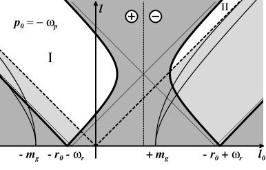
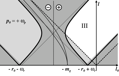
Figure 6: Allowed domains in the $(l_{o},l)$ plane for $p_{o}=\pm\omega_{p}$. The area shaded in dark gray is excluded by the delta function constraints. The areas shaded in light gray are above the light-cone (dotted lines). The light curves are the transverse and longitudinal mass shells of the thermalized gluon. The vertical dotted line is the separation between $\epsilon(p_{o})\epsilon(r_{o}+l_{o})=+1$ and $\epsilon(p_{o})\epsilon(r_{o}+l_{o})=-1$.

The above two inequalities may be rewritten as

$$\sqrt{(r-l)^{2}+M^{2}_{\infty}}\leq l_{o}+r_{o}{\rm\ \ or\ \ }l_{o}+r_{o}\leq-\sqrt{(r-l)^{2}+M^{2}_{\infty}}\qquad\qquad$$ (44)

$$-\sqrt{(r+l)^{2}+M^{2}_{\infty}}\leq l_{o}+r_{o}\leq\sqrt{(r+l)^{2}+M^{2}_{\infty}}$$ (45)

The result of these inequalities is shown in Fig. 6, where the regions excluded by the requirement $\cos\theta^{\prime}\in[-1,+1]$ are shaded in dark gray. In order to make the comparison easier with the case of static photons, we have also reproduced the boundaries of the allowed region for that case (i.e. the frontiers that one obtains in the limit $M_{\infty}\to 0$). One can see that the old boundaries are asymptotes for the news ones. Again, we have three regions allowed by the above two inequalities for $L^{2}\leq 0$. Again, regions I and III give the same contribution, as can be seen by the change of variables $P\to-R-L$ performed at an earlier stage of the calculation. From now on, we will drop region I and multiply by a factor $2$ the contribution of region III. We start the discussion with the study of region III (bremsstrahlung processes) and then turn to region II ($q\bar{q}$ annihilation with scattering in the plasma, see Fig. 4). As will be seen, this region can no longer be neglected, contrary to the case of soft photon production.

4.2 Bremsstrahlung

Since the delta function $\delta(P^{2}-M^{2}_{\infty})$ makes more convenient the choice of $p\equiv||{\tenimbf p}||$ as an independent variable (instead of $r$), the quantities $-r_{o}\pm\omega_{r}$ that appear on the previous figure are to be understood as functions of $p$ and the angle $\theta$ between ${\tenimbf p}$ and ${\tenimbf q}$. Therefore, this restriction of the allowed phase space is in fact a constraint that relates the independent variables $p$,$\theta$,$l$ and $l_{o}$. In the following, doing the integration over $\theta$ first will prove to be convenient since, due to collinear divergences, the result of this angular integral controls the order of magnitude of the result. If $u\equiv 1-\cos\theta$ is the variable over which we integrate first, then the bounds on $u$ depend on the other variables $l,l_{o}$ and $p$ because of the identities of Eqs. (45-a) and (45-b). In particular, the inequality Eq. (45-a) can be written in terms of $u\equiv 1-\cos\theta$:

$$u\leq{{(p+q)^{2}-(\sqrt{(r_{o}+l_{o})^{2}-M^{2}_{\infty}}-l)^{2}}\over{2pq}}\;,$$ (46)

which gives if one assumes that $l_{o}$ and $l$ are soft

$$u\leq\left({{l}\over{p}}+{{l}\over{q}}\right)(1-x)\;,$$ (47)

where we denote $x\equiv l_{o}/l$. As a consequence, since the relevant values of the momentum $l$ are controlled by thermal masses of order $gT$, this upper bound is of order $g$.

It is now worth giving expressions for the denominators that enter in the rate, since they are potentially dangerous when the photon is emitted collinearly to the quark. To that purpose, we need also another angular variable, which is left unconstrained by the previous considerations. This variable can be the azimuthal angle $\phi$ between ${\tenimbf q}$ and ${\tenimbf l}$ when projected on a plane orthogonal to ${\tenimbf r}$. Therefore, if we denote $\theta^{\prime\prime}$ the angle between ${\tenimbf q}$ and ${\tenimbf l}$, we can calculate this angle by

$$\cos\theta^{\prime\prime}=\cos\theta_{r}\cos\theta^{\prime}+\sin\theta_{r}\sin\theta^{\prime}\cos\phi\;,$$ (48)

where $\theta_{r}$ is the angle between ${\tenimbf r}$ and ${\tenimbf q}$. This last angle is not independent of $\theta$, to which it can be related by

$$r\sin\theta_{r}=p\sin\theta$$ (49)

$$r\cos\theta_{r}=p\cos\theta+q\;;$$ (50)

so that Eq. (48) can be rewritten as

$$\cos\theta^{\prime\prime}={p\over{r}}\left(\cos\theta\cos\theta^{\prime}+\sin\theta\sin\theta^{\prime}\cos\phi\right)+{q\over r}\cos\theta^{\prime}\;.$$ (51)

Using only the variables $u=1-\cos\theta$, $p$, $l$ and $x=l_{o}/l$, we can write[19]

$$R^{2}-M^{2}_{\infty}\approx 2pq\left[u+{{M^{2}_{\infty}}\over{2p^{2}}}\right]\;,$$ (52)

and

$$\int\limits_{0}^{2\pi}{{d\phi}\over{(P+L)^{2}-M^{2}_{\infty}}}\approx{{2\pi(p+q)}\over{2qp^{2}\left[\left(u+{{M^{2}_{\infty}}\over{2p^{2}}}+{{L^{2}}\over{2p^{2}}}\right)^{2}-{{L^{2}}\over{p^{2}}}{{M^{2}_{\infty}}\over{p^{2}}}\right]^{1/2}}}\;,$$ (53)

where we performed the integration over $\phi$ at this stage since this denominator is the only place where $\phi$ appears at the dominant order. As one can see, the first formula remains exactly the same as in the case of soft real photons [19], while the second one is only slightly modified by an extra $(p+q)/p$ factor. As a consequence, the discussion made in [19] concerning the enhancement that one gets when performing the $u$ integral is still valid. In particular, the terms where both denominators are present are enhanced by a factor of order $p^{2}/M^{2}_{\infty}$, while those where only one of them appear will get only a logarithm of this quantity.

Again, our starting point is Eq. (2.3). The order of magnitude of each term is evaluated by taking into account the fact that the momentum $Q$ is now hard, as well as the quark momentum. Moreover, we must take into account the enhancement by a factor of order $1/g^{2}$ for terms having two denominators. Since the emitted photon is assumed to be real, we have $Q^{2}=0$. Therefore, one can check that only one term dominates in this matrix element:

$$-8L^{2}{{\overline{R}{}^{\rho}\overline{R}{}^{\sigma}+\overline{P}{}^{\rho}\overline{P}{}^{\sigma}}\over{\overline{R}{}^{2}(\overline{P+L}){}^{2}}}\;,$$ (54)

which is again the same as in the case of soft real photons.

Since the relevant values of $u$ are of order $M^{2}_{\infty}/p^{2}\sim g^{2}$, we have

$$r_{o}-\omega_{r}\approx{{pq}\over{p+q}}\left[u+{{M^{2}_{\infty}}\over{2p^{2}}}\right]{\rm\ \ for\ }{p_{o}=+\omega_{p}}\;.$$ (55)

Therefore, one can see in Fig. 6 that the extra requirement $L^{2}\leq 0$ does not restrict significantly region III due to Eq. (55) (this is a result already obtained in [19] according to which the kinematics confines the phase space to the $L^{2}\leq 0$ region in the collinear limit if $L$ is soft).

Since the term to consider is the same, and since the denominators have very similar expressions, it is completely straightforward to reproduce the calculation that has been performed in [19]. The only minor difference lies in the contraction of $\overline{R}{}^{\rho}\overline{R}{}^{\sigma}+\overline{P}{}^{\rho}\overline{P}{}^{\sigma}$ with the projectors, which gives a factor $p^{2}+r^{2}$ approximated by $p^{2}+(p+q_{o})^{2}$ in the collinear limit. Introducing the dimensionless quantities:

$$w\equiv{{-L^{2}}\over{M^{2}_{\infty}}}$$ (56)

$$\widetilde{I}_{{}_{T,L}}(x)\equiv{{{\rm Im}\,\Pi_{{}_{T,L}}(x)}\over{M^{2}_{\infty}}}\;,\qquad\widetilde{R}_{{}_{T,L}}(x)\equiv{{{\rm Re}\,\Pi_{{}_{T,L}}(x)}\over{M^{2}_{\infty}}}\;,$$ (57)

we find

$$\halign to=0.0pt{\@eqnsel\hskip\@centering$\displaystyle{#}$&\global\@eqcnt\@ne\hskip 2\arraycolsep\hfil${#}$\hfil&\global\@eqcnt\tw@\hskip 2\arraycolsep$\displaystyle{#}$\hfil&\llap{#}\cr 0.0pt plus 1000.0pt$\displaystyle{&10.0pt\hfil${&10.0pt$\displaystyle{{\rm Im}\,\Pi^{{}^{AR}}{}_{\mu}{}^{\mu}(Q)\approx{{e^{2} g^{2} N C_{{}_{F}}}\over{\pi^{4}}}(J_{{}_{T}}-J_{{}_{L}}) {{T}\over{q_{o}^{2}}}\;\\ &\hbox to0.0pt{\hss&\qquad\times\int\limits_{0}^{+\infty}dp\;(p^{2}+(p+q_{o})^{2})\left[n_{{}_{F}}(p)-n_{{}_{F}}(p+q_{o})\right]\;,&(58)\cr}}}}}$$

where we denote

$$J_{{}_{T,L}}\equiv\int\limits_{0}^{1}{{dx}\over{x}}\;\widetilde{I}_{{}_{T,L}}(x)\;\int\limits_{0}^{+\infty}dw\;{{\sqrt{w/{w+4}}\,{\rm tanh}^{-1}\sqrt{w/{w+4}}}\over{(w+\widetilde{R}_{{}_{T,L}}(x))^{2}+(\widetilde{I}_{{}_{T,L}}(x))^{2}}}\;.$$ (59)

As one can see, the integral over $x$ and $w$ can be factorized out of the expression and is the same as in the case of soft real photons [19]. In this previous work, we noticed that the integral over the gluon momentum could potentially be singular when the gluon is transverse, but is regularized by the quark thermal mass instead of the gluon thermal mass as one might expect. The interpretation of this result is in fact rather simple. Indeed, a close look at kinematics shows that the delta functions $\delta(P^{2}-M^{2}_{\infty})$ and $\delta((R+L)^{2}-M^{2}_{\infty})$ become incompatible in the limit $L\to 0$ if $M^{2}_{\infty}>0$. Therefore, the quark thermal mass prevents an infrared divergence by reducing to zero the region of phase space where this divergence can occur. The only major difference with [19] concerns the integral over $p$, because of the fact that $q_{o}$ is now hard. Nevertheless, we can still give a rather compact expression for this integral in terms of poly-logarithms:

$$\halign to=0.0pt{\@eqnsel\hskip\@centering$\displaystyle{#}$&\global\@eqcnt\@ne\hskip 2\arraycolsep\hfil${#}$\hfil&\global\@eqcnt\tw@\hskip 2\arraycolsep$\displaystyle{#}$\hfil&\llap{#}\cr 0.0pt plus 1000.0pt$\displaystyle{&10.0pt\hfil${&10.0pt$\displaystyle{\int_{0}^{\infty}dp (p^{2}+(p+q_{o})^{2}) [n_{F}(p) - n_{F}(p+q_{0})] \\ &\hbox to0.0pt{\hss&\qquad=T^{3}\left[3\zeta(3)+{{\pi^{2}}\over{6}}{{q_{o}}\over{T}}+\left({{q_{o}}\over{T}}\right)^{2}\ln(2)\right.\\&&\qquad\qquad+4\,{\rm Li\kern 1.0pt}_{3}(-e^{-|q_{o}|/T})+2{{q_{o}}\over{T}}\,{\rm Li\kern 1.0pt}_{2}(-e^{-|q_{o}|/T})\\&&\qquad\qquad\left.-\left({{q_{o}}\over{T}}\right)^{2}\ln(1+e^{-|q_{o}|/T})\right]\;,&(60)\cr}}}}}$$

where the poly-logarithm functions are defined via

$${\rm Li\kern 1.0pt}_{a}(z)\equiv\sum\limits_{n=1}^{+\infty}{{z^{n}}\over{n^{a}}}\;.$$ (61)

Eq. (4.2) simplifies in the limit of extremely hard photons $q_{o}\gg T$:

$$\int\limits_{0}^{+\infty}dp\;(p^{2}+(p+q_{o})^{2})\left[n_{{}_{F}}(p)-n_{{}_{F}}(p+q_{o})\right]\mathrel{\mathop{\kern 0.0pt\approx}\limits_{q_{o}\gg T}}q_{o}^{2}T\ln(2)\;.$$ (62)

Therefore, in this asymptotic regime, we find for the production rate of hard real photons:

$$\left.{{dN}\over{dtd{\tenimbf x}}}\right|_{\rm bremss}\mathrel{\mathop{\kern 0.0pt\approx}\limits_{q_{o}\gg T}}2{{d{\tenimbf q}}\over{\pi^{5}}}NC_{{}_{F}}\alpha{{\alpha_{{}_{S}}}}\Big{(}\sum_{f}e_{f}^{2}\Big{)}{{T^{2}}\over{q_{o}}}e^{-q_{o}/T}(J_{{}_{T}}-J_{{}_{L}})\ln(2)\;,$$ (63)

where $e_{f}$ is the electric charge of the quark of flavor $f$ expressed in units of the electron charge.

Besides this simple asymptotic result, it is worth adding that Eqs. (4.2) and (4.2) provide a generalization of the analogous formula of [19]. Indeed, the result we provide in the present paper for the bremsstrahlung contribution to real photon production is valid over the whole range of photon energies, and in particular reduces to Eq. (55) of [19] in the limit of soft $q_{o}$.

4.3 $q\bar{q}$ annihilation with scattering

The discussion of the contribution of region II can be carried out in a similar way. We recall that $p_{o}=-\omega_{p}<0$ so that Eq. (52) becomes

$$R^{2}-M^{2}_{\infty}\approx-2pq\left[v+{{M^{2}_{\infty}}\over{2p^{2}}}\right]\;,$$ (64)

with the notation $v\equiv 1+\cos\theta$. For hard enough $q_{o}$, the statistical weight $n_{{}_{F}}(p_{o})-n_{{}_{F}}(p_{o}+q_{o})$ is equal to $1$ for $-q_{o}\leq p_{o}\leq 0$ and equals $0$ everywhere else. Therefore, we can restrict to the range $0\leq p\leq q_{o}$ and we check that Eq. (53) remains valid except for the changes $u\to v$ and $q+p\to q-p$. The enhancement mechanism in the terms that contain the two denominators goes through as before due to their behavior near $v\sim g^{2}$.

Such terms are dominated by the region where $v\sim g^{2}$, which enables us to obtain $-r_{o}-\omega_{r}\approx-2(q_{o}-p)$ and $-r_{o}+\omega_{r}\sim{\cal O}(g^{2}T)$. As a consequence, the boundaries in the $(l_{o},l)$ plane are $-1\leq x\leq 1$ and $0\leq l\leq 2(q-p)/(1-x)$, where $x\equiv l_{o}/l$. Therefore, the integral over $l$ and $x$ gives the same factor $J_{{}_{T}}-J_{{}_{L}}$ as before. The integral over $p$ in Eq. (4.2) is now to be replaced by

$$\int\limits_{0}^{q_{o}}dp\,(p^{2}+(q_{o}-p)^{2})={{2q_{o}^{3}}\over{3}}\;,$$ (65)

which leads to the following asymptotic contribution for the region II:

$$\left.{{dN}\over{dtd{\tenimbf x}}}\right|_{\rm II}\mathrel{\mathop{\kern 0.0pt\approx}\limits_{q_{o}\gg T}}{2\over 3}{{d{\tenimbf q}}\over{\pi^{5}}}NC_{{}_{F}}\alpha{{\alpha_{{}_{S}}}}\Big{(}\sum_{f}e_{f}^{2}\Big{)}{{q_{o}T}\over{q_{o}}}e^{-q_{o}/T}(J_{{}_{T}}-J_{{}_{L}})\;.$$ (66)

Therefore, it appears that region II dominates over bremsstrahlung in the asymptotic regime.

4.4 Comparison with previous results

The production rate of hard real photons has already been calculated at the one-loop order in [10, 11] as an application of the effective theory based on the resummation of hard thermal loops. We now compare the contribution of bremsstrahlung obtained above with their result. For hard real photons, the predictions of [10] are

$$\left.{{dN}\over{dtd{\tenimbf x}}}\right|_{\rm 1-loop}\mathrel{\mathop{\kern 0.0pt\approx}\limits_{q_{o}\gg T}}{{d{\tenimbf q}}\over{8\pi^{2}}}NC_{{}_{F}}\alpha{{\alpha_{{}_{S}}}}\Big{(}\sum_{f}e_{f}^{2}\Big{)}{{T^{2}}\over{q_{o}}}e^{-q_{o}/T}\ln\left({{cq_{o}}\over{\alpha_{{}_{S}}T}}\right)\;,$$ (67)

with the constant $c\approx 0.23$.

It is worth recalling here that the quantities $J_{{}_{T,L}}$ that appear in Eqs. (63) and (66) are functions of the ratio $M_{\infty}/m_{\rm g}$ when $Q^{2}=0$, i.e. depend only on $N$ and $N_{{}_{F}}$. For $N=3$ colors and $N_{{}_{F}}=2$ light flavors, we can evaluate numerically $J_{{}_{T}}\approx 4.45$ and $J_{{}_{L}}\approx-4.26$. The following plot shows a comparison of bremsstrahlung, $q\bar{q}$ annihilation with scattering, and one-loop contributions.

Figure 7: Comparison of various contributions to ${\rm Im}\,\Pi{}^{\mu}_{\mu}(Q)$ for a hard real photon. The comparison is made for $N=3$ colors and $N_{{}_{F}}=2$ flavors. The value taken for the coupling constant is $g=0.5$.

In this figure, the bremsstrahlung contribution is taken from Eq. (4.2); for the region II, we use the asymptotic result obtained for large $q_{o}$ , and the one-loop result is a numerical evaluation of the diagrams considered in [10]. The value used here for the coupling constant is $g=0.5$. We can see that the bremsstrahlung is the dominant contribution for the smaller values $q_{o}$, whereas the region II becomes dominant for hard enough $q_{o}$. For intermediate photon energies (around $T$), the three contributions have equivalent orders of magnitude. For higher values of the coupling constant $g$, the relative importance of the one-loop contribution tends to decrease. We can also see that the sum of the three contributions is significantly above the one-loop contribution considered alone.

5 Conclusions and perspectives

We have discussed the production of a real photon or of a lepton pair in a hot quark-gluon plasma in thermal equilibrium. We assumed that the plasma is described by thermal Quantum Chromodynamics and we worked in the framework of the effective theory obtained after resummation of hard thermal loops. We have shown that, at leading order in $gT$, it is necessary to include the one-loop as well as the two-loop diagrams. The one-loop diagrams of the effective theory correctly account for the contribution of soft fermion momenta in the loop, whereas in the two-loop diagrams hard momenta play a dominant role.

Many physical processes are contained in the effective theory calculated up to two-loop order. To simplify, it can be said that, at one-loop, scattering processes mediated by (soft) fermion exchanges are of paramount importance for the emission of the photon. The corresponding photon production rate consequently strongly depends on the soft fermion thermal mass $m_{{}_{F}}$. On the other hand, the two-loop topologies account, among other possibilities, for bremsstrahlung processes where the photon is emitted by a hard quark scattering in the plasma via a (space-like) gluon exchange: in that case the rate is proportional to the square of the gluon mass $m_{\rm g}$. We have calculated the contribution of such processes.

For the production a soft virtual photon ($q_{o}\sim gT$, ${\tenimbf q}={\tenimbf 0}$) the bremsstrahlung processes largely dominate over the one-loop result in the range $q_{o}\mathchar 5166\relax m_{{}_{F}}$. For the case of real photon production an interesting enhancement phenomenon occurs in the bremsstrahlung processes. Because of the vanishing photon mass, the fermion propagators become infinite when a quasi forward-scattered quark emits a collinear photon: the singularities are regularized by an interplay between the thermal masses of the fermion and the gluon. It was seen before that this leads to an enhancement by a factor $1/g^{2}$ of the bremsstrahlung contributions to the real soft photon rate so that the two-loop diagrams entirely dominate over the one-loop contribution. On the other hand, the bremsstrahlung production of a hard real photon occurs at the same order in $g$ as the one-loop result. A rather simple analytic expression, valid for soft, hard and ultra-hard photon has been derived. For ultra-hard photons, another process becomes dominant, consisting of $q\bar{q}$ annihilation where one of the fermions undergoes a scattering in the medium. In all cases, the calculated two-loop contributions considerably increase the rate of photon or lepton pair emission. Our results can easily be numerically extended to cover, on the one hand, the case of a soft lepton pair at non-vanishing momentum, and on the other hand, the case of lepton pairs produced at large momentum with a small invariant mass. All the features of the present results should survive in these more general situations.

A word of caution should be given concerning the bremsstrahlung contribution to the soft virtual photon rate. The result shows a sensitivity to a hard space-like gluon and therefore one may suspect that the extrapolation of the effective gluon propagator in the hard region is not complete: to be consistent may require taking into account three-loop diagrams in very much the same way two-loop diagrams were needed besides the one-loop diagram with a hard space-like fermion propagator. On the contrary, for the case of a real photon emission, the bremsstrahlung rate is sensitive only to soft gluon momenta, and the calculation is therefore expected to be complete.

Our study does not cover all the physical processes included in the two-loop diagrams. In particular, the contribution with a time-like gluon should be added. However such processes when the gluon is hard are already contained in the one-loop diagram: counterterms should therefore be included. To do this will be a very interesting practical exercise in the use of the effective theory up to two-loop.

Appendix A Hard thermal loops and counterterms

When using effective theories based on the summation of hard thermal loops at higher orders, there is potentially a possibility to have multiple counting of thermal corrections that should be there only once.

As a first illustration of this problem in a trivial context, let us use the example of a massless real scalar field with a $\lambda^{2}\phi^{4}$ interaction in $4$ dimensions. The Lagrangian of such a model is

$${\cal L}\equiv{1\over 2}\partial_{\mu}\phi\partial^{\mu}\phi-{{\lambda^{2}}\over{4!}}\phi^{4}\;.$$ (68)

After the calculation of the one-loop tadpole, one realizes that this diagram – a hard thermal loop in the terminology of [3] – generates a thermal mass $m=\lambda T\surd 24$ that can be important for the phenomenology of soft modes. Therefore, the idea of the HTL resummation is to include this thermal mass in an effective Lagrangian

$${\cal L}_{\rm eff}\equiv{1\over 2}\partial_{\mu}\phi\partial^{\mu}\phi-{1\over 2}m^{2}\phi^{2}-{{\lambda^{2}}\over{4!}}\phi^{4}\;,$$ (69)

which is the Lagrangian of a real scalar field of mass $m$.

Let us assume now that one uses this effective theory instead of the bare one to calculate the same tadpole diagram. The result would be

$$\Pi={{\lambda^{2}T^{2}}\over{24}}\left(1-{3\over\pi}{m\over T}-{3\over{2\pi^{2}}}\left({m\over T}\right)^{2}\ln\left({m\over T}\right)+\cdots\right)=m^{2}(1+{\cal O}(\lambda))\;,$$ (70)

and since we start now from a propagator with squared mass $m^{2}$, the resummation of the self-energy $\Pi$ would lead us to a propagator with a squared mass $2m^{2}(1+{\cal O}(\lambda))$, approximately twice larger than the correct thermal mass. Obviously, the above result arises due to multiple countings of the same thermal correction. Stated differently, this is a consequence of the fact that this effective theory is more than a mere reordering of the perturbative expansion of the bare theory since its Lagrangian is different. To solve this problem, one must write

$${\cal L}={\cal L}_{\rm eff}+{\cal L}_{\rm ct}{\ \ \rm with\ \ }{\cal L}_{\rm ct}\equiv{1\over 2}m^{2}\phi^{2}\;,$$ (71)

and treat the counterterm ${\cal L}_{\rm ct}$ as an interaction term, just like $\lambda^{2}\phi^{4}/4!$. The effect of this counterterm is of course to subtract at higher order the thermal corrections that had already been included at the tree level via the effective Lagrangian, in order to avoid multiple countings. For instance, in the above example, the correct answer for the tadpole $\Pi$ when one takes care of the counterterm is

$$\Pi={{\lambda^{2}T^{2}}\over{24}}\left(1-{3\over\pi}{m\over T}-{3\over{2\pi^{2}}}\left({m\over T}\right)^{2}\ln\left({m\over T}\right)+\cdots\right)-m^{2}={\cal O}(\lambda m^{2})$$ (72)

which is a perturbative correction to the thermal mass found at the previous step, as it should be. When this counterterm is taken properly into account, the effective theory is nothing more than a reordering of the perturbative expansion, since the overall Lagrangian remains unmodified.

This problem also arises in effective gauge theories, where the situation is a bit more complicated since we need there an infinite series – one for each hard thermal loop – of non-local counterterms. These counterterms are defined to be the opposite of the HTL contribution to the corresponding function. Then, to a given diagram obtained in the effective theory, one should add the diagrams obtained by collapsing each loop in turn and replacing it by the corresponding counterterm. In order to be more definite, let us consider the example of the two-loop diagram of figure 1-[b]. In the figure 8, we have represented next to the one-loop contribution to the polarization tensor of the photon some of its two-loop corrections.

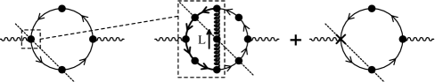
Figure 8: Some corrections to the one-loop contribution (left diagram) to the photon polarization tensor. A black dot denotes an effective propagator or vertex. Crosses are HTL counterterms. The boldface loop may reproduce what is already included in the one-loop diagram when its momentum is hard.

It should be clear from the figure that when the boldface loop of the second diagram carries a hard momentum, then this loop reproduces the HTL part of the effective vertex in the dotted box already included at one-loop, plus new sub-dominant perturbative corrections. The purpose of the third diagram is precisely to subtract a quantity equal to the HTL contribution to this vertex, so that what remains constitutes only new contributions. The net effect of this procedure is thus to reorder the terms of the perturbative expansion.

Let us now explain why, despite their conceptual importance, the counterterms do not contribute in the case of bremsstrahlung. As said in section 2, the contributions of bremsstrahlung to photon production come from two-loop diagrams in which the gluon propagator is cut, and where one retains only the Landau damping part ($L^{2}<0$) of the cut gluon propagator. Technically, the gluon included in the 3-point HTL that appears on the third diagram of Figure 8 is a bare one, and therefore its discontinuity has support totally included in the time-like region. As a consequence, the diagram with counterterms contributes only in the region of phase-space where $L^{2}\geq 0$, and cannot contribute to bremsstrahlung. Even if they are not a worry in the case of bremsstrahlung, it was important to discuss the potential effect of counterterms since, having shown that the second diagram gives an important contribution, it is not enough to conclude that the two-loop order is important, as it may be canceled by counterterms.

Appendix B Phase space considerations

The purpose of this appendix is to emphasize the importance of being in a thermal bath in order to have a hard phase space for the quark loop. This is indeed crucial in the calculations performed in the previous sections since this feature of the diagrams considered in this paper enables them to be of the same order of magnitude as one-loop diagrams. In order to make the following discussion more intuitive, let us first transform the bremsstrahlung photon production rate in a way that separates more clearly the phase space from the amplitude of the process producing the photon. The tools to do that have already been presented in [19] (see the section devoted to the comparison with semi-classical methods), so that we only give the result here:

$$\halign to=0.0pt{\@eqnsel\hskip\@centering$\displaystyle{#}$&\global\@eqcnt\@ne\hskip 2\arraycolsep\hfil${#}$\hfil&\global\@eqcnt\tw@\hskip 2\arraycolsep$\displaystyle{#}$\hfil&\llap{#}\cr 0.0pt plus 1000.0pt$\displaystyle{&10.0pt\hfil${&10.0pt$\displaystyle{\left.{{dN}\over{dtd{\tenimbf x}}}\right|_{\rm bremss}={{d{\tenimbf q}}\over{(2\pi)^{3}2q_{o}}}\int{{d^{4}P}\over{(2\pi)^{4}}} \int{{d^{4}K}\over{(2\pi)^{4}}} \int{{d^{4}L}\over{(2\pi)^{4}}}\\ &\hbox to0.0pt{\hss&\qquad\times\raise-19.91692pt\hbox to142.26378pt{{\leavevmode\resizebox{142.26378pt}{}{\includegraphics{fig09.ps}}}}\\&&\qquad\times 2\pi\delta(P^{2}-M^{2}_{\infty})\,2\pi\delta((R+L)^{2}-M^{2}_{\infty})\\&&\qquad\times 2\pi\delta(K^{2}-M^{2}_{\infty})\,2\pi\delta((K+L)^{2}-M^{2}_{\infty})\\&&\qquad\times n_{{}_{F}}(r_{o}+l_{o})n_{{}_{F}}(k_{o})[1-n_{{}_{F}}(p_{o})][1-n_{{}_{F}}(k_{o}+l_{o})]\;,&(73)\cr}}}}}$$

where $R\equiv P+Q$. This formula tells us that in order to calculate the contribution of some process to the photon production rate, we just have to integrate the amplitude squared of this process over the phase space of unobserved particles (here, the incoming and outgoing quarks). When doing this integration, the external particles are put on their mass shells, and accompanied by the appropriate statistical weight. The main advantage of this formula is that it exhibits a clear separation in two factors: the amplitude squared of the process producing the photon, and the phase space of the quarks. Therefore, this formula can be used to separate the estimation of the order of magnitude of the diagram in two steps: the order of magnitude of the amplitude, and the size of the phase space over which it must be integrated.

Looking at this formula, it is clear that the effect of the thermal bath appears only in the phase space. Indeed, the amplitude that appears in Eq. (B) is nothing but a zero temperature one (it does not contain any statistical weight). Stated differently, if, instead of looking at photon production by a thermal bath, we were looking at bremsstrahlung photon production in p-p collisions (i.e. the two scattering quarks come from protons in colliding beams), the statistical factors of incoming quarks would have to be replaced by structure functions of a quark inside a proton, and the statistical weights of outgoing quarks would be replaced by 1. This difference is precisely the point which makes the thermal bath dramatically different from the p-p collision. Indeed, in the case of the thermal bath, the statistical functions have a support which is 3-dimensional since the plasma is an isotropic medium. On the other hand, the structure function of the quark inside protons of the beam is vanishing if the quark has a direction different from that of the beam. This will make a difference when one performs the integral over the momentum $p$. Indeed, if one has something like $\int dpp^{n}f(p)$ in the case of the thermal bath, the integral would be $\int dpp^{n-2}f(p)$ for the case of p-p collisions. As a consequence, the integral over the quark momentum is more likely to be sensitive to hard momenta in the case of the thermal bath. Therefore, even if it is not a rigorous proof, these considerations show why some higher order processes which are not dominant at zero temperature may become dominant in a plasma, due to a bigger size for their phase space.

Moreover, Eq. (B) may help to understand why two-loop contributions may be as important as one-loop ones. Indeed, it shows that the final order of magnitude of a contribution results from a competition between two effects. The first one is the order of magnitude of the amplitude, which usually becomes smaller when the number of loops increases since the number of coupling constants increases also. The second aspect of the problem is the size of the phase space, since it may happen that due to kinematical constraints, the one-loop phase space is much smaller than the two-loop one. Both effects can compensate so that two-loop diagrams contribute also at the dominant level. This is precisely what happens in the case of photon production by a plasma: the one-loop phase space is soft due to kinematical constraints, while the two-loop thermal phase space can be hard (as explained above, this is possible because we are in an isotropic medium). Therefore, the smallness of the two-loop amplitude is compensated by the size of the two-loop phase space.

References

- [1] R.D. Pisarski, Phys. Rev. Let. 63, 1129 ().
- [2] R.D. Pisarski, Physica A 158, 146 ().
- [3] E. Braaten, R.D. Pisarski, Nucl. Phys. B 337, 569 ().
- [4] E. Braaten, R.D. Pisarski, Nucl. Phys. B 339, 310 ().
- [5] J. Frenkel, J.C. Taylor, Nucl. Phys. B 334, 199 ().
- [6] J. Frenkel, J.C. Taylor, Nucl. Phys. B 374, 156 ().
- [7] E. Braaten, R.D. Pisarski, T.C. Yuan, Phys. Rev. Lett. 64, 2242 ().
- [8] R. Baier, S. Peigné, D. Schiff, Z. Phys. C 62, 337 ().
- [9] P. Aurenche, T. Becherrawy, E. Petitgirard, Preprint ENSLAPP-A-452/93, hep-ph/9403320.
- [10] R. Baier, H. Nakkagawa, A. Niegawa, K. Redlich, Z. Phys. C 53, 433 ().
- [11] J.I. Kapusta, P. Lichard, D. Seibert, Phys. Rev. D 44, 2774 ().
- [12] J. Cleymans, V.V. Goloviznin, K. Redlich, Phys. Rev. D 47, 989 ().
- [13] J. Cleymans, V.V. Goloviznin, K. Redlich, Z. Phys. C 59, 495 ().
- [14] V.V. Goloviznin, K. Redlich, Phys. Lett. B 319, 520 ().
- [15] R. Baier, Y.L. Dokshitzer, A.H. Mueller, S. Peigné, D. Schiff, Nucl. Phys. B 478, 577 ().
- [16] R. Baier, Y.L. Dokshitzer, A.H. Mueller, S. Peigné, D. Schiff, Nucl. Phys. B 483, 291 ().
- [17] H.A. Weldon, Phys. Rev. D 28, 2007 ().
- [18] C. Gale, J.I. Kapusta, Nucl. Phys. B 357, 65 ().
- [19] P. Aurenche, F. Gelis, R. Kobes, E. Petitgirard, Z. Phys. C 75, 315 ().
- [20] P. Aurenche, F. Gelis, R. Kobes, E. Petitgirard, Phys. Rev. D 54, 5274 ().
- [21] M.A. van Eijck, R. Kobes, Ch.G. van Weert, Phys. Rev. D 50, 4097 ().
- [22] R.L. Kobes, G.W. Semenoff, Nucl. Phys. B 260, 714 ().
- [23] R.L. Kobes, G.W. Semenoff, Nucl. Phys. B 272, 329 ().
- [24] F. Gelis, Nucl. Phys. B 508, 483 ().
- [25] Work in progress.
- [26] F. Flechsig, A.K. Rebhan, Nucl. Phys. B 464, 279 ().
- [27] H.A. Weldon, Phys. Rev. D 26, 1394 ().
- [28] N.P. Landsman, Ch.G. van Weert, Phys. Rep. 145, 141 ().
- [29] V.V. Klimov, Sov. Phys. JETP 55, 199 ().
- [30] V.V. Klimov, Sov. J. Nucl. Phys. 33, 934 ().