Constraints for hypothetical interactions from
a recent demonstration of the Casimir force
and some possible improvements

Abstract

The Casimir force is calculated in the configuration of a spherical lens and a disc of finite radius covered by $Cu$ and $Au$ thin layers which was used in a recent experiment. The correction to the Casimir force due to finiteness of the disc radius is shown to be negligible. Also the corrections are discussed due to the finite conductivity, large-scale and short-scale deviations from the perfect shape of the bounding surfaces and the temperature correction. They were found to be essential when confronting the theoretical results with experimental data. Both Yukawa-type and power-law hypothetical forces are computed which may act in the configuration under consideration due to the exchange of light and/or massless elementary particles between the atoms of the lens and the disc. New constraints on the constants of these forces are determined which follow from the fact that they were not observed within the limits of experimental errors. For Yukawa-type forces the new constraints are up to 30 times stronger than the best ones known up today. A possible improvement of experimental parameters is proposed which gives the possibility to strengthen constraints on Yukawa-type interactions up to $10^{4}$ times and on power-law interactions up to several hundred times.

I INTRODUCTION

During the past decades the Casimir effect [1] found a large number of applications in different branches of physics (see monograph [2] and references therein). Among them the applications should be mentioned in statistical physics, in elementary particle physics (e.g. in the bag model in QCD or in Kaluza-Klein theories) and in the cosmology of the early Universe. From the point of view of quantum field theory the Casimir effect is a specific type of vacuum polarization which appears by quantizing the theory in restricted volumes or in spaces with non-trivial topology. This polarization results from a change of the spectrum of zero-point oscillations in the presence of nontrivial boundary conditions. For the case of the electromagnetic vacuum between two uncharged metallic boundaries, separated by a small gap $a$, the Casimir effect leads to the appearance of an attractive force acting on them depending on $a$ and on the fundamental constants $\hbar$ and $c$ only. Such attractive force may be alternatively explained as a retarded van der Waals force between the two bodies whose conducting surfaces are responsible for the Casimir force.

The Casimir force was firstly measured by Sparnaay [3] for metallic surfaces. For dielectric bodies the corresponding forces had been measured more frequently, see [4–7]. The relative error in the force measurements was about 100% in [3] and in the range of $(10-20)\%$ in [4–7].

As it was shown in Refs. [8,9] the Casimir force between macroscopic bodies is very sensitive to the presence of additional hypothetical interactions predicted by unified gauge theories, supersymmetry and supergravity. According to these theories interactions of two atoms arise due to the exchange of light or massless elementary particles between them (for example, scalar axions, graviphotons, dilatons, arions and others). Their effective interatomic potentials may be described by Yukawa- and power-laws. After the integration over the volume of two macro-bodies one obtains more complicated laws for their interaction potentials. It was rather unexpected that quite strong constraints for the characteristic constants of these laws may be found from the experiments on Casimir force measurements.

The constraints under consideration may be found also from other precision experiments, e.g., from Eötvös-, Galileo- and Cavendish-type experiments, from the measurements of the van der Waals forces, transition probabilities in exotic atoms etc (for a collection of references on long-range hypothetical forces see [10]).

According to the results of [8,11,12] the Casimir force measurements of [4–7] lead to the strongest constraints on the constants of Yukawa-type hypothetical interactions with a range of action of $10^{-8}{\,\mbox{\rm m}}<\lambda<10^{-4}{\,\mbox{\rm m}}$. For $\lambda<10^{-8}{\,\mbox{\rm m}}$ the best constraints follow from the measurements of van der Waals forces in atomic force microscopy and of transition probabilities in exotic atoms [13]. For $\lambda>10^{-4}{\,\mbox{\rm m}}$, as it was shown in [11,12], they follow from Cavendish- and Eötvös-type experiments [14–17].

In [9] the constraints were obtained from the Casimir effect on the constants of power-law potentials decreasing with distance as $r^{-n}$. For $n$ = 2, 3 and 4 they turn out to be the best ones up to 1987 (compare [18]). In [19] a bit stronger constraints on the power-law interaction were obtained from the Cavendish-type experiment of Ref. [14].

Recently, a new experiment was performed [20] on the measurement of the Casimir force between two metallized surfaces of a flat disc and a spherical lens. The absolute error of the force measurements in [20] was $\Delta F\approx 10^{-11}N$ for distances $a$ between the disc and the lens in the range $1{\,\mu{\mbox{\rm m}}}\leq a\leq 6{\,\mu{\mbox{\rm m}}}$. This was the first measurement of the Casimir force between metallic surfaces after [3]. For the distance $a\approx 1{\,\mu{\mbox{\rm m}}}$ the value of the Casimir force in the configuration under consideration is $F_{C}\approx-3.1\times 10^{-10}\,$N. This means that the relative error of the force measurement at $1{\,\mu{\mbox{\rm m}}}$ in [20] is about $\delta\approx 3\%$ (note that with increasing $a$ the value of $\delta$ increases quickly). In [20] the active surfaces of the disc and the lens were covered by thin layers of copper and gold. The use of heavier metals for the test bodies is preferable for obtaining stronger constraints on hypothetical interactions. This follows from the fact that the value of the hypothetical forces increases proportionally to the square of the density.

The aim of the present paper is to give an accurate calculation of different hypothetical forces which might appear in the configuration used in the experiment [20]. Also, the corrections to the Casimir force due to distortions of the surfaces, to edge effects, finite conductivity and non-zero temperature will be analysed. On this base new constraints on the hypothetical interactions will be reliably calculated, which follow from the results of [20], as well as their possible improvement. The corresponding constraints which result for the masses of light elementary particles are also discussed. Some preliminary results of this kind were obtained in [21] for Yukawa-type interactions and in [22] for power-law forces. However, in [21,22] the corrections to the Casimir force were not discussed and different possibilities suggested by experiment [20] were not accounted for in full detail.

The paper is organized as follows. In Sec. II we discuss the expression for the Casimir force in a configuration of a plane disc and a lens and different corrections to it are considered taking into account the finiteness of the diameter of the disc. Sec. III is devoted to the calculation of Yukawa-type forces in this configuration. In Sec. IV analogous results are obtained for the case of power-law hypothetical forces. Sec. V contains a careful derivation of the new constraints on the constants of Yukawa- and power-law interactions which follow from the experiment performed in [20]. The possible improvement of the experiment [20] is considered in Sec. VI. For Yukawa-type interactions it gives the possibility to make the constraints about several thousand times stronger. This considerable strengthening of constraints may be achieved also for the power-law hypothetical interactions. Sec. VII contains the conclusions and some discussions. In the Appendix the reader will find a number of mathematical details concerning the calculation of the Casimir and hypothetical forces.

II THE CASIMIR FORCE BETWEEN
A DISC AND A LENS INCLUDING
CORRECTIONS

The scheme of the configuration used in the recent demonstration of the Casimir force [20] is shown in Fig. 1. The Casimir force was measured between the metallized surfaces of a flat disc (with radius $L=1.27{\,\mbox{\rm cm}}$ and thickness $D=0.5{\,\mbox{\rm cm}}$) and a spherical lens (with curvature radius $R=11.3{\,\mbox{\rm cm}}$ and height $H=0.18{\,\mbox{\rm cm}}$). The separation between them was varied from $a=0.6{\,\mu{\mbox{\rm m}}}$ up to $6{\,\mu{\mbox{\rm m}}}$. Both bodies were made out of quartz and covered by a continuous layer of copper with $\Delta=0.5{\,\mu{\mbox{\rm m}}}$ thickness. The surfaces which faces each other were covered additionally with a layer of gold of the same thickness. Note that the penetration depth of the electromagnetic field into gold is approximately $\delta_{0}\approx 0.08{\,\mu{\mbox{\rm m}}}\ll\Delta$. By this reason when calculating the Casimir force one may consider the interacting bodies as being made of gold as a whole.

The experimental data obtained in [20] has been confronted with the theoretical result

$$F_{C}^{(0)}(a)=-\frac{\pi^{3}}{360}\,R\,\frac{\hbar c}{a^{3}}.$$ (1)

This formula is valid for the configuration of a small lens situated near the center of a large (strictly speaking, infinite) disc at zero temperature. It was first derived in [4] and reobtained by different methods afterwards (see, e.g., [2, 23]). In Ref. [20], (1) was derived from the well known result for two infinite plane parallel plates using the Proximity Force Theorem [24]. Note, that according to our notations the attractive forces are negative and repulsive ones are positive.

Actually, in the experiment [20] the diameter of the disc was not much larger, but even smaller than the size of the lens. Therefore it is of great interest to calculate corrections to Eq. (1) due to the finite disc size. For this purpose we use the approximation method developed earlier for the calculation of the Casimir force and which may be applied to the case of two bodies with arbitrarily shaped surfaces [2, 23, 25, 26]. According to this method the potential of the Casimir force can be obtained by summation of the retarded van der Waals interatomic potentials over all pairs of atoms in the bodies under consideration with a subsequent multiplicative renormalization (the latter takes into account a large amount of the non-additivity of these forces). The method was tested and successfully applied in the above cited papers. As a result the Casimir force may be calculated according to:

$$F_{C}(a)=-\frac{\partial U_{C}(a)}{\partial a},$$ (2)

$$U_{C}(a)=-\Psi(\varepsilon_{1},\varepsilon_{2})\int\limits_{V_{1}}d^{3}r_{1}\int\limits_{V_{2}}d^{3}r_{2}\,\frac{1}{r_{12}^{7}},$$ (3)

where $r_{12}$ is the distance between the atoms belonging to the first and to the second body, $\Psi(\varepsilon_{1},\varepsilon_{2})$ is a tabulated function depending on the static dielectric permittivities of the test bodies (for its explicit form see [2, 26, 27]). In the limit of perfectly conducting surfaces (which is of interest here) $\varepsilon_{1},\varepsilon_{2}\to\infty$ and $\Psi(\varepsilon_{1},\varepsilon_{2})\to\pi\hbar c/24$. In [26] the relative error of the values given by (2) was examined. It was shown to be of the order of $0,01\%$ for configurations which do not much differ from that of two plane parallel plates. This is just the case in the experiment [20], because only the top of the lens and its vicinity contribute essentially to the Casimir force.

The integration in (2) for the configuration of a lens and a disc (Fig. 1) may be performed analytically. For this reason we introduce a spherical system of coordinates with the origin in the curvature center of the lens. The angle $\theta$ is counted from the horizontal axis directed out of the origin to the left (see Fig. 1). Then Eq. (2) for $U_{C}$ takes the form

$$U_{C}(a)=-\Psi(\varepsilon_{1},\varepsilon_{2})\int\limits_{0}^{2\pi}\!d\varphi_{1}\!\int\limits_{0}^{\theta_{1}}\!\sin\vartheta_{1}\,d\vartheta_{1}\!\!\!\int\limits_{R_{\min}^{\prime}(\vartheta_{1})}^{R}\!\!\!r_{1}^{2}\,dr_{1}$$ (4)

$$\phantom{aaaaaa}\times\int\limits_{0}^{2\pi}\!d\varphi_{2}\!\int\limits_{0}^{\theta_{2}}\!\sin\vartheta_{2}\,d\vartheta_{2}\!\!\!\int\limits_{R_{\min}(\vartheta_{2})}^{R_{\max}(\vartheta_{2})}\!\!\!r_{2}^{2}\,dr_{2}\,\frac{1}{r_{12}^{7}},$$ (5)

where the integration limits are defined as follows (prime is used for the lens)

$$R_{\min}^{\prime}(\vartheta_{1})=\frac{R-H}{\cos\vartheta_{1}},\quad\theta_{1}=\arccos\frac{R-H}{R},$$ (6)

$$R_{\min}(\vartheta_{2})=\frac{R+a}{\cos\vartheta_{2}},\quad R_{\max}(\vartheta_{2})=\frac{R+a+D}{\cos\vartheta_{2}},$$ (7)

$$\theta_{2}=\arccos\frac{R+a}{\sqrt{(R+a)^{2}+L^{2}}}\approx\arccos\frac{R}{\sqrt{R^{2}+L^{2}}}.$$ (8)

Using the potential energy in the form of (5) with the integration limits (6) we slightly change the experimental configuration converting the disc into a part of a truncated cone (the corresponding addition to the disc volume is $\Delta V/V\approx D/R\approx 4\%$). This increasing takes place, however, near the outer boundary of the disc and practically does not influence the result for the Casimir force.

The integrals in (3) may be calculated along the lines presented in Appendix. Putting $k=3$ in (A11) we obtain the result for the power-law interaction with a power equal to $2k+1=7$:

$$U_{C}(a)=-\Psi(\varepsilon_{1},\varepsilon_{2})\frac{16\pi^{2}}{5}\int\limits_{0}^{\theta}\!\sin\vartheta\,d\vartheta$$ (9)

$$\phantom{aaaaaaaa}\times\int\limits_{R_{\min}^{\prime}(\vartheta)}^{R}\!\!\!\!dr_{1}\!\!\!\!\int\limits_{R_{\min}(\vartheta)}^{R_{\max}(\vartheta)}\!\!\!\!dr_{2}\,\frac{r_{1}^{2}\,r_{2}^{2}}{(r_{1}+r_{2})^{2}(r_{2}-r_{1})^{5}},$$ (10)

where $\theta=\min(\theta_{1},\theta_{2})$.

We rewrite (5) in a more convenient form by introducing the new variables $t=\cos\vartheta$, $x_{1}=tr_{1}$, $x_{2}=tr_{2}$ and using Eq. (A6) for $r_{1}r_{2}$:

$$U_{C}(a)=-\Psi(\varepsilon_{1},\varepsilon_{2})\frac{\pi^{2}}{5}\int\limits_{t_{0}}^{1}\!tdt\!\int\limits_{R-H}^{Rt}\!\!dx_{1}\!\!\int\limits_{R+a}^{R+a+D}\!\!dx_{2}\,\frac{(x_{1}+x_{2})^{2}}{(x_{2}-x_{1})^{5}},$$ (11)

where $t_{0}=\max(R/\sqrt{R^{2}+L^{2}},(R-H)/R)$. It is seen that the value of $t_{0}$ depends on the relative sizes of the lens and of the disc. If $L\leq\sqrt{2RH}$ one has $t_{0}\approx 1-L^{2}/(2R^{2})$. But if $L>\sqrt{2RH}$, then $t_{0}=(R-H)/R$ and the Casimir force does not depend on a further increase of $L$ due to the quick decreasing of the retarded van der Waals potential with distance.

Calculating the Casimir force by the first equation of (2) the integration with respect to $x_{2}$ is removed resulting in the expression

$$F_{C}(a)=-\Psi(\varepsilon_{1},\varepsilon_{2})\frac{\pi^{2}}{5}\int\limits_{t_{0}}^{1}\!t\,dt\!\int\limits_{R-H}^{Rt}\!\!dx_{1}\left[\frac{(x_{1}+R+a)^{2}}{(R+a-x_{1})^{5}}\right.$$ (12)

$$\phantom{aaaaaaa}-\left.\frac{(x_{1}+R+a+D)^{2}}{(R+a+D-x_{1})^{5}}\right].$$ (13)

This result coincides with (1) if we consider the limit $L,\varepsilon_{1,2}\to\infty$ (infinite disc made of a perfect metal) keeping the lowest order in the small parameter $a/R$. Integrating eq. (7) explicitly we find that the main contribution to the result, depending on the size of the disc, appears at the third order in $a/R$ [28]

$$F_{C}(a)\approx F_{C}^{(0)}(a)\left[1-\frac{a^{3}}{R^{3}}\frac{1}{(1-t_{0})^{3}}\right].$$ (14)

For the parameters of experiment [20] the inequality $L\leq\sqrt{2RH}$ holds. In this case it follows from (8)

$$F_{C}(a)\approx F_{C}^{(0)}(a)\left(1-8\frac{a^{3}R^{3}}{L^{6}}\right).$$ (15)

It is easily seen from (15) that the correction to the Casimir force due to the finite size of the disc does not exceed its maximal value $6\times 10^{-7}$ which is achieved for $a=6{\,\mu{\mbox{\rm m}}}$. That is why one actually may neglect this correction when confronting the measurements of the Casimir force with the theory.

Let us discuss the corrections to the Casimir force (1) which are significant for a small spatial separation of the lens and the disc, $a\approx 1{\,\mu{\mbox{\rm m}}}$. It is reasonable to start with the corrections due to the finite conductivity of the metal covering the test bodies [2,29–31]. It is well known that for $a$ in the micrometer range the penetration depth of the electromagnetic field into the metal is frequency independent and inversely proportional to the effective plasma frequency of the electrons: $\delta_{0}=c/\omega_{p}$. For two plane parallel metallic plates the corrections for the Casimir force due to the finite conductivity were found in [29–31] (see also [2]). Up to the first two orders in the relative penetration depth $\delta_{0}/a$ the result is:

$$F_{C}(a)\approx F_{C}^{(0)}(a)\left(1-\frac{16}{3}\,\frac{\delta_{0}}{a}+24\,\frac{\delta_{0}^{2}}{a^{2}}\right).$$ (16)

Using the Force Proximity Theorem [24] it is not difficult to modify (10) for the configuration of a lens and a disc:

$$F_{C}(a)\equiv F_{C}^{(0)}(a)+\Delta_{\delta_{0}}F_{C}^{(0)}(a)$$ (17)

$$\phantom{aaaaaa}\approx F_{C}^{(0)}(a)\left(1-4\,\frac{\delta_{0}}{a}+\frac{72}{5}\,\frac{\delta_{0}^{2}}{a^{2}}\right).$$ (18)

Note that the first order correction in (17) was found firstly in [20]. The plus sign in front of it in [20] is a misprint (this is also clear from general considerations according to which $F_{C}(a)$ is constant in sign for all $\delta_{0}$ and tends to zero in the formal limit $\delta_{0}\to\infty$ so that the correction should be negative [2]).

For gold, as it was mentioned above, $\delta_{0}\approx 0.08{\,\mu{\mbox{\rm m}}}$ and for $a=1{\,\mu{\mbox{\rm m}}}$ the correction to the Casimir force $F_{C}^{(0)}$ due to the finite conductivity achieves $23\%$ of $F_{C}^{(0)}$. The behaviour of this correction (in relative units) with increasing $a$ is shown in Fig. 2 (curve 1). The experimental data in [20] do not support the presence of corrections of the result (1) being so large (let us remind that the relative error of the force measurements at $1{\,\mu{\mbox{\rm m}}}$ was about $3\%$ and with such an accuracy Eq. (1) was confirmed).

According to [20] the reason of this contradiction is the inapplicability of (16), (17) for gold (in more detail, the approximation for the effective dielectric permittivity which was used in [30] to derive the first order correction in (16) does not take into account the large imaginary part of the refraction index for gold [20]). On the other hand the corrections due to the finite conductivity (which are in agreement with [30]) were found in [31] (see also [2]) in a more general impedance approach without use of the dielectric permittivity. Consequently, Eqs. (16) and (17) are still valid for gold covered surfaces and the contradiction with the experimental data is still present. The most reasonable way to resolve this problem is to take into account the corrections of the Casimir force due to the deviations of the surfaces from the perfect shape (in [20] such corrections were not discussed).

Let us now assume that the surfaces of the lens and of the disc are covered by some distortions with characteristic amplitudes $A_{1}$ and $A_{2}$, correspondingly. Then the general result for the Casimir force up to second order in the relative amplitudes of the distortions takes the form

$$F_{C}(a)\approx F_{C}^{(0)}(a)\left[1+C_{10}\frac{A_{1}}{a}+C_{01}\frac{A_{2}}{a}\right.$$ (19)

$$\phantom{aaaaaaaa}\left.+C_{20}\left(\frac{A_{1}}{a}\right)^{2}+C_{02}\left(\frac{A_{2}}{a}\right)^{2}+C_{11}\frac{A_{1}A_{2}}{a^{2}}\right],$$ (20)

where the explicit expressions for the coefficients in terms of the functions describing the shape of distortions were found in [23].

For small stochastic distortions, instead of (12), one has [23]

$$F_{C}(a)\equiv F_{C}^{(0)}(a)+\Delta_{d}F_{C}^{(0)}(a)$$ (21)

$$\phantom{aaaaaa}\approx F_{C}^{(0)}(a)\left[1+6\left(\frac{\delta_{1}}{a}\right)^{2}+6\left(\frac{\delta_{2}}{a}\right)^{2}\right],$$ (22)

where $\delta_{1,2}$ are the dispersions of the stochastic perturbations on the surfaces. The same result is valid for the non-stochastic short-scale distortions regardless of the specific shape of the functions describing them. Here $\delta_{1,2}$ should be substituted by $A_{1,2}/\sqrt{2}$. Note that the result (21) can be obtained using the Proximity Force Theorem [24] from the corresponding result for two plane parallel plates [32].

Speculating that the characteristic values of the dispersion is of order $\delta_{i}\approx 0.1{\,\mu{\mbox{\rm m}}}$ we get from (21) a positive correction to the Casimir force which is equal to $12\%$ of $F_{C}^{(0)}(a)$ for $a=1{\,\mu{\mbox{\rm m}}}$. In Fig. 2 (curve 2) the dependence of this correction on $a$ is shown in relative units.

Note that the first order correction resulting from (19) appears only in the case when there are some large-scale deviations of boundary surfaces from the perfect shape for which the non-perturbed force is calculated. Using a realistic estimation of $A_{i}/a\approx 0.1$ for $a\approx 1{\,\mu{\mbox{\rm m}}}$ the first order correction in (19) may amount as much as $30\%$ of $F_{C}^{(0)}$ [23]. In the experiment [20] the radius of the lens $R=(11.3\pm 0.1){\,\mbox{\rm cm}}$ was determined with a rather large absolute error. Consequently, a large-scale deviation of the surface of the lens from the perfect shape could have taken place. A special inspection of the lens used in [20], which was not done, is required to determine the actual size (and shape) of the large-scale deviations. After that it would be possible to calculate the coefficients $C_{10}$ and $C_{01}$ and the corresponding correction to the Casimir force.

Together with the correction $\Delta_{d}F_{C}^{(0)}(a)$ due to the short-scale distortions it may easily compensate the negative correction to the Casimir force due to the finite conductivity of gold. This is possibly the reason why in [20] neither corrections to the finite conductivity nor to the surface distortions were observed at $a\approx 1{\,\mu{\mbox{\rm m}}}$.

One more correction to the Casimir force (1) is due to the non-zero temperature $T$. It is calculated, e.g., in [33] for two plane parallel metallic plates (see also [2]). For a lens and a disc the corresponding result may be obtained by the use of the Proximity Force Theorem and has the form

$$F_{C}(a)\equiv F_{C}^{(0)}(a)+\Delta_{T}F_{C}^{(0)}(a)$$ (23)

$$=F_{C}^{(0)}(a)\left[1+\frac{720}{\pi^{2}}f(\xi)\right].$$ (24)

Here $\xi=k_{B}Ta/(\hbar c)$, $k_{B}$ is Boltzmann’s constant and

$$f(\xi)=\frac{1}{4\pi^{2}}\sum\limits_{l,m=1}^{\infty}\frac{(2\xi)^{4}}{\left[l^{2}+m^{2}(2\xi)^{2}\right]^{2}}$$ (25)

$$\phantom{a}=\frac{1}{4\pi^{2}}\left\{\sum\limits_{l=1}^{\infty}\left[\frac{2\pi\xi^{3}}{l^{3}}\frac{\cosh\frac{\pi l}{2\xi}}{\sinh\frac{\pi l}{2\xi}}+\frac{(\pi\xi)^{2}}{l^{2}}\sinh^{-2}\left(\frac{\pi l}{2\xi}\right)\right]\right.$$ (26)

$$\phantom{aaaaaaaaaaaa}\left.-\frac{4\pi^{4}}{45}\xi^{4}\vphantom{\left[\frac{\cosh\frac{\pi l}{2\xi}}{\sinh\frac{\pi l}{2\xi}}\right]}\right\}.$$ (27)

The relative value of the temperature corrections, calculated with (23), (25) is shown in Fig. 2 (curve 3) in dependence on $a$. It is seen that for $a=1{\,\mu{\mbox{\rm m}}}$ it is approximately $2.7\%$ of $F_{C}^{(0)}$. But for $a=6{\,\mu{\mbox{\rm m}}}$ the temperature correction is $\Delta_{T}F_{C}^{(0)}=1.74F_{C}^{(0)}$.

Fig. 2 will be used in Secs. V, VI which are devoted to obtain stronger constraints on the constants of hypothetical interactions from the Casimir force measurements (the other forces which may contribute in the experiment, i.e. electric one should be subtracted to get the result for the Casimir force with possible corrections discussed above, see [20]).

III THE YUKAWA-TYPE HYPOTHETICAL
INTERACTION BETWEEN A DISC
AND A LENS

The Yukawa potential between two atoms of the interacting bodies may be represented in the form

$$V_{Yu}=-\alpha\,N_{1}\,N_{2}\,\hbar\,c\,\frac{1}{r_{12}}{e}^{-r_{12}/\lambda},$$ (28)

where $\alpha$ is a dimensionless interaction constant, $\lambda=\hbar/(mc)$ is the Compton wavelength of a hypothetical particle which is responsible for the rise of new interactions, and $N_{i}$ are the numbers of nucleons in the atomic nuclei; they are introduced in (16) to make $\alpha$ independent on the sort of atoms.

The potential energy of hypothetical interaction in the configuration of experiment [20] (see Fig. 1) may be obtained as the additive sum of the potentials (16) with appropriate atomic densities of the lens and the disc materials

$$U_{Yu}(a)=-\alpha\,\frac{\hbar c}{m_{p}^{2}}\sum\limits_{i,j=1}^{3}\rho_{i}^{\prime}\rho_{j}U_{Yu}^{(i,j)}(a),$$ (29)

$$U_{Yu}^{(i,j)}(a)=\int\limits_{V_{i}^{\prime}}d^{3}r_{1}\int\limits_{V_{j}}d^{3}r_{2}\,\frac{1}{r_{12}}\,{e}^{-r_{12/\lambda}}.$$ (30)

Here $\rho_{i}^{\prime}$, $V_{i}^{\prime}$ ($i=1,2,3$) are the densities and volumes of the lens and the covering metallic layers ($\rho_{j}$, $V_{j}$ are the same for the disc). The proton mass $m_{p}$ appeared due to the use of usual densities instead of the atomic ones. In numerical calculations of Sec. V the values $\rho_{1}^{\prime}=2.23\,$g/cm³, $\rho_{1}=2.4\,$g/cm³, $\rho_{2}^{\prime}=\rho_{2}=8.96\,$g/cm³, $\rho_{3}^{\prime}=\rho_{3}=19.32\,$g/cm³ [20] will be used.

The hypothetical force between lens and disc can be computed as the derivative

$$F_{Yu}(a)=-\frac{\partial U_{Yu}(a)}{\partial a}.$$ (31)

The integration (17) can be performed most simply in a spherical coordinate system described in Sec. II (see Fig. 1). In these coordinates the multiple integral from (17) takes the form

$$U_{Yu}^{(i,j)}(a)=\int\limits_{0}^{2\pi}\!d\varphi_{1}\!\int\limits_{0}^{\theta_{1}}\!\sin\vartheta_{1}\,d\vartheta_{1}\!\!\int\limits_{R_{i,\min}^{\prime}}^{R_{i,\max}^{\prime}}\!\!\!r_{1}^{2}\,dr_{1}$$ (32)

$$\phantom{aaaaaa}\times\int\limits_{0}^{2\pi}\!d\varphi_{2}\!\int\limits_{0}^{\theta_{2}}\!\sin\vartheta_{2}\,d\vartheta_{2}\!\!\int\limits_{R_{j,\min}}^{R_{j,\max}}\!\!\!r_{2}^{2}\,dr_{2}\,\frac{1}{r_{12}}\,{e}^{-r_{12}/\lambda}.$$ (33)

The quantities $\theta_{1}$, $\theta_{2}$ were defined in (4), the other integration limits are (as above by the prime the lens parameters are notated)

$$R_{1,\min}^{\prime}=\frac{R-H}{\cos\vartheta_{1}},\quad R_{1,\max}^{\prime}=R_{2,\min}^{\prime}=R-\Delta_{1}^{\prime}-\Delta_{2}^{\prime},$$ (34)

$$R_{2,\max}^{\prime}=R_{3,\min}^{\prime}=R-\Delta_{2}^{\prime},\qquad R_{3,\max}^{\prime}=R,$$ (35)

$$R_{1,\min}=R_{2,\max}=\frac{R+a+\Delta_{1}+\Delta_{2}}{\cos\vartheta_{2}},$$ (36)

$$R_{1,\max}=\frac{R+a+D}{\cos\vartheta_{2}},\qquad R_{3,\min}=\frac{R+a}{\cos\vartheta_{2}},$$ (37)

$$R_{2,\min}=R_{3,\max}=\frac{R+a+\Delta_{2}}{\cos\vartheta_{2}}.$$ (38)

For generality the thicknesses of metallic layers on the lens and on the disc are permitted to be different.

To calculate the integrals in (19) it is convenient to use the expansion into a series of spherical harmonics [34]

$$\frac{{e}^{-r_{12}/\lambda}}{r_{12}}=\frac{4\pi}{\sqrt{r_{1}r_{2}}}\sum\limits_{l=0}^{\infty}{I}_{l+\frac{1}{2}}\left(\frac{r_{1}}{\lambda}\right)\,{K}_{l+\frac{1}{2}}\left(\frac{r_{2}}{\lambda}\right)\,$$ (39)

$$\phantom{aaaaaa}\times\sum\limits_{m=-l}^{l}{Y}_{lm}^{\ast}(\vartheta_{1},\varphi_{1})\,{Y}_{lm}(\vartheta_{2},\varphi_{2}),$$ (40)

where ${I}_{\nu}(z)$, ${K}_{\nu}(z)$ are Bessel functions of imaginary argument. For large arguments ($z\gg 1$) one has

$${I}_{l+\frac{1}{2}}(z)\approx\frac{1}{\sqrt{2\pi z}}\,{e}^{z},\qquad{K}_{l+\frac{1}{2}}(z)\approx\sqrt{\frac{\pi}{2z}}\,{e}^{-z}.$$ (41)

Let us consider separately the cases of small and large parameter $\lambda$. In (21) the condition $z\gg 1$ corresponds to $\lambda\ll r_{1},r_{2}$ which is valid when $\lambda\ll R$ (actually $\lambda$ must be less than the lowest size of the interacting bodies, i.e. $\lambda<H$ in the configuration under consideration). Substituting the asymptotics (22) into the right-hand side of (21) and taking into account the completeness relation for spherical harmonics (A9) we obtain for $\lambda<H$:

$$\frac{{e}^{-r_{12}/\lambda}}{r_{12}}\approx\frac{2\pi\lambda}{r_{1}\,r_{2}}\,{e}^{r_{1}/\lambda}\,{e}^{-r_{2}/\lambda}$$ (42)

$$\phantom{aaaaaaa}\times\delta(\varphi_{1}-\varphi_{2})\,\delta(\cos\vartheta_{1}-\cos\vartheta_{2}).$$ (43)

Substituting (23) into (19) we get two different situations depending on the value of index $i$. If $i=2,3$ (the integration is over the layers covering the lens) the integration limits in $r_{1}$ do not depend on $\vartheta$:

$$U_{Yu}^{(i,j)}(a)=4\pi^{2}\lambda\int\limits_{0}^{\theta}\!\sin\vartheta\,d\vartheta\!\!$$ (44)

$$\phantom{aaaaaaaaa}\times\int\limits_{R_{i,\min}^{\prime}}^{R_{i,\max}^{\prime}}\!\!\!r_{1}\,dr_{1}\,{e}^{r_{1}/\lambda}\!\!\!\!\int\limits_{R_{j,\min}(\vartheta)}^{R_{j,\max}(\vartheta)}\!\!\!\!r_{2}\,dr_{2}\,{e}^{-r_{2}/\lambda},$$ (45)

where $\theta=\min(\theta_{1},\theta_{2})$.

It is convenient to consider the force $f_{Yu}^{(i,j)}(a)=-\partial U_{Yu}^{(i,j)}(a)/\partial a$ instead of the potential energy (24). This gives the possibility to remove the integration with respect to $r_{2}$. Integrating with respect to the variables $r_{1}$ and $\vartheta$ in a standard way [35] one gets for $i=2,3$ and $j=1,2,3$:

$$f_{Yu}^{(i,j)}(a)=4\pi^{2}\lambda^{3}{e}^{-a_{ij}/\lambda}(R-\lambda)\left(1-{e}^{-\Delta_{i-1}^{\prime}/\lambda}\right)$$ (46)

$$\phantom{aaaaa}\times\left\{1-{e}^{-BR/\lambda}-{e}^{-d_{j}/\lambda}\left[1-{e}^{-(R+d_{j})B/\lambda}\right]\right\}.$$ (47)

Here the following notations are used:

$$a_{33}=a,\qquad a_{32}=a+\Delta_{1},\qquad a_{31}=a+\Delta_{1}+\Delta_{2},$$ (48)

$$a_{23}=a+\Delta_{2}^{\prime},\qquad a_{22}=a+\Delta_{2}+\Delta_{2}^{\prime},$$ (49)

$$a_{21}=a+\Delta_{2}+\Delta_{1}^{\prime}+\Delta_{2}^{\prime},$$ (50)

$$d_{1}=D-\Delta_{1}-\Delta_{2}\approx D,\qquad d_{2}=\Delta_{1},\qquad d_{3}=\Delta_{2},$$ (51)

$$B=\min\left(\frac{L^{2}}{2R^{2}},\frac{H}{R}\right).$$ (52)

Now we consider the second situation where the integration in (19) is over the lens itself ($i=1$). Here the quantity $U_{Yu}^{(1,j)}(a)$ has the same form as in (24) but with integration limit $R_{1,\min}^{\prime}$ depending on $\vartheta$. Considering the force instead of potential energy and performing the integration by the use of tabulated formulas [35] we find the result:

$$f_{Yu}^{(1,j)}(a)=4\pi^{2}\lambda^{3}{e}^{-a_{1j}/\lambda}\left\{(R-\lambda)\vphantom{\left[{e}^{-(H+d_{j})B/\lambda}\right]}\right.$$ (53)

$$\phantom{aaaa}\times\left[1-{e}^{-BR/\lambda}-{e}^{-d_{j}/\lambda}\left(1-{e}^{-(R+d_{j})B/\lambda}\right)\right]$$ (54)

$$\phantom{aaaa}-{e}^{-H/\lambda}\left[A_{1}-A_{2}{e}^{-BH/\lambda}-A_{3}^{(j)}{e}^{-d_{j}/\lambda}\vphantom{{e}^{-(H+d_{j})B/\lambda}}\right.$$ (55)

$$\phantom{aaaaaaaaa}\left.\left.+A_{4}^{(j)}{e}^{-d_{j}/\lambda}{e}^{-(H+d_{j})B/\lambda}\right]\right\}.$$ (56)

Here the following notations are introduced:

$$a_{11}=a+\Delta_{1}+\Delta_{2}+\Delta_{1}^{\prime}+\Delta_{2}^{\prime},$$ (57)

$$a_{12}=a+\Delta_{2}+\Delta_{1}^{\prime}+\Delta_{2}^{\prime},$$ (58)

$$a_{13}=a+\Delta_{1}^{\prime}+\Delta_{2}^{\prime},$$ (59)

$$A_{1}=\frac{R}{H}\left[\frac{(R-H)(H+\lambda)}{H}-\lambda\right],$$ (60)

$$A_{2}=\frac{R}{H}\left[\frac{(R-H)(H+\lambda t_{0})}{H}-\lambda\right],$$ (61)

$$A_{3}^{(j)}=\frac{R+d_{j}}{H+d_{j}}\left[\frac{(R-H)(H+d_{j}+\lambda)}{H}-\lambda\right],$$ (62)

$$A_{4}^{(j)}=\frac{R+d_{j}}{H+d_{j}}\left[\frac{(R-H)(H+d_{j}+\lambda t_{0})}{H}-\lambda\right],$$ (63)

$t_{0}$ is defined in explanations to (6).

The complete value of the hypothetical force, according to (17), (18), may be presented in the form:

$$F_{Yu}=-\alpha\,\frac{\hbar c}{m_{p}^{2}}\sum\limits_{i,j=1}^{3}\rho_{i}^{\prime}\,\rho_{j}\,f_{Yu}^{(i,j)},$$ (64)

where $f_{Yu}^{(i,j)}$ are defined in (25), (27). The expressions (25), (27), (29) will be used in Secs. V,VI for calculating constraints on Yukawa-type hypothetical interactions.

Note that for the extremely small $\lambda{\,{\scriptscriptstyle{\stackrel{{\scriptstyle<}}{{\sim}}}}\,}a$ the expression (29) may be additionally simplified:

$$F_{Yu}=-\alpha\frac{\hbar c}{m_{p}^{2}}4\pi^{2}\lambda^{3}{e}^{-a/\lambda}R$$ (65)

$$\phantom{aaaa}\times\left[\rho_{1}^{\prime}{e}^{-(\Delta_{1}^{\prime}+\Delta_{2}^{\prime})/\lambda}+\rho_{2}^{\prime}{e}^{-\Delta_{2}^{\prime}/\lambda}+\rho_{3}^{\prime}\right]$$ (66)

$$\phantom{aaaaaa}\times\left[\rho_{1}{e}^{-(\Delta_{1}+\Delta_{2})/\lambda}+\rho_{2}{e}^{-\Delta_{2}/\lambda}+\rho_{3}\right].$$ (67)

Exactly this result (for equal thicknesses of the covering metallic layers) follows in the limit of small $\lambda$ from the formula derived in [21] for the configuration of a lens and an infinite disc. Thus for $\lambda{\,{\scriptscriptstyle{\stackrel{{\scriptstyle<}}{{\sim}}}}\,}a$ the finiteness of the disc size does not influence the value of the hypothetical force. At the same time for larger $\lambda$ it is necessary to take into account the finite sizes of the disc (unlike the case when we calculated the Casimir force in Sec. II).

Let us start with the case of large $\lambda$ ($\lambda\gg R$). Now we may neglect the exponent in Eq. (16). As a result the interatomic potential does not depend on $\lambda$ any more and behaves as $1/r_{12}$. For this potential the hypothetical force between a lens and a disc was calculated in [9] under the assumption that the disc area is infinitely large. Such suggestion is not reliable for the potential under consideration due to its slow decrease with the distance. The general method developed in the Appendix for the potentials of the form $r_{12}^{-(2k+1)}$ with $k\geq 1$ also should be modified to include the case $k=0$. We will take into account that for large $\lambda$ the covering metallic layers practically do not contribute to the result. By this reasoning one may integrate directly over the lens and the disc volumes. As a result in a spherical coordinate system used above the expression for the hypothetical force is:

$$F_{Yu}\approx-\alpha\,\frac{\hbar c}{m_{p}^{2}}\,\rho_{1}^{\prime}\,\rho_{1}\int\limits_{0}^{2\pi}\!d\varphi_{1}\int\limits_{0}^{2\pi}\!d\varphi_{2}\int\limits_{0}^{\theta_{1}}\!\sin\vartheta_{1}\,d\vartheta_{1}$$ (68)

$$\phantom{aa}\times\int\limits_{0}^{\theta_{2}}\!\sin\vartheta_{2}\,d\vartheta_{2}\!\!\int\limits_{R_{\min}^{\prime}}^{R}\!\!\!r_{1}^{2}\,dr_{1}\!\!\!\int\limits_{R_{\min}}^{R_{\max}}\!\!\!r_{2}^{2}\,dr_{2}\,\frac{r_{2}\cos\vartheta_{2}-r_{1}\cos\vartheta_{1}}{r_{12}^{3}}.$$ (69)

The calculational details for integration in (31) are given in Appendix. The result is:

$$F_{Yu}\approx-\alpha\frac{\hbar c}{m_{p}^{2}}\rho_{1}^{\prime}\rho_{1}2\pi^{2}L^{2}DH$$ (70)

$$\phantom{aaaa}\times\left[1-\frac{L^{2}}{4RH}\left(\ln\frac{D+H}{D}+\frac{H}{D}\ln\frac{D+H}{H}\right)\right].$$ (71)

In the intermediate range between $\lambda<H$ and $\lambda\gg R$ the integration in (17) was performed numerically. For this purpose algorithm 698 from netlib [36] was used. It is an adaptive multidimensional integration, the FORTRAN program is called DCUHRE. A large number of function calls (about $5\times 10^{6}$) for $\lambda\geq 2.3\times 10^{-4}\,$m was necessary in order to obtain reliable results. For smaller values $\lambda$ the program does not work. The results of numerical calculations are in good agreement with the analytical ones (see Secs. V,VI).

IV CALCULATION OF A POWER-LAW
INTERACTION

In this Section the force is calculated which may act in the configuration of experiment [20] due to power-law hypothetical interactions. The power-law potential between two atoms belonging to a lens and a disc is

$$V_{n}=-\lambda_{n}\,N_{1}\,N_{2}\,\hbar\,c\,\frac{1}{r_{12}}\left(\frac{r_{0}}{r_{12}}\right)^{n-1}.$$ (72)

Here $\lambda_{n}$ is a dimensionless constant and $r_{0}=1$F$\,=10^{-15}\,$m is introduced for the proper dimensionality of potentials with different $n$ [18].

The potential energy of the lens and the disc (see Fig. 1) due to a hypothetical interaction is an additive sum of the potentials (33) with appropriate atomic densities. It can be written in a form analogous to (17)

$$U_{n}(a)=-\lambda_{n}\frac{\hbar\,c\,r_{0}^{n-1}}{m_{p}^{2}}\sum\limits_{i,j=1}^{3}\rho_{i}^{\prime}\rho_{j}U_{n}^{(i,j)}(a),$$ (73)

$$F_{n}(a)=-\frac{\partial U_{n}(a)}{\partial a}.$$ (74)

The quantities $U_{n}^{(i,j)}$ here are defined by the same integrals as in (17) where instead of $\exp(-r_{12}/\lambda)$ the function $1/r_{12}^{n-1}$ should be substituted.

At first we consider the case $n=3$. Here the result for $U_{3}^{(i,j)}$ is given by (A11) with $k=1$. We rewrite it by using (A6) for $r_{1}r_{2}$ and introducing the new variables $t=\cos\vartheta$, $x_{1}=tr_{1}$, $x_{2}=tr_{2}$

$$U_{3}^{(i,j)}(a)=\pi^{2}\int\limits_{t_{0}}^{1}\frac{dt}{t^{3}}\int\limits_{tR_{i,\min}^{\prime}}^{tR_{i,\max}^{\prime}}\!\!dx_{1}\!\!\int\limits_{tR_{j,\min}}^{tR_{j,\max}}\!\!dx_{2}\,\frac{(x_{1}+x_{2})^{2}}{x_{2}-x_{1}},$$ (75)

where $t_{0}$ is defined in the explanation to (6).

Calculating the force, one can eliminate the integration with respect to $x_{2}$:

$$F_{3}^{(i,j)}(a)=-\frac{\partial U_{3}^{(i,j)}(a)}{\partial a}$$ (76)

$$\phantom{a}=\pi^{2}\!\int\limits_{t_{0}}^{1}\frac{dt}{t^{3}}\!\int\limits_{tR_{i,\min}^{\prime}}^{tR_{i,\max}^{\prime}}\!\!\!\!dx_{1}\left[\frac{(x_{1}+tR_{j,\max})^{2}}{tR_{j,\max}-x_{1}}-\frac{(x_{1}+tR_{j,\min})^{2}}{tR_{j,\min}-x_{1}}\right].$$ (77)

Performing the integration in (36) for different values of $i,j$ to lowest order in the small parameters $H/R$, $L^{2}/(2R^{2})$, $D/R$, $\Delta_{i}^{\prime}/H$, $\Delta_{j}/D$, $a/H$, $a/D$ and $a/L$, and substituting the results into (34), we obtain:

$$F_{3}(a)=-4\pi^{2}\lambda_{3}\frac{\hbar\,c\,r_{0}^{2}}{m_{p}^{2}}\,R$$ (78)

$$\phantom{aa}\times\left\{\rho_{1}^{\prime}\rho_{1}\left[D\ln\frac{2RD+\tilde{L}^{2}}{2RD}+\frac{\tilde{L}^{2}}{2R}\ln\frac{(2RD+\tilde{L}^{2})H}{\tilde{L}^{2}(H+D)}\right]\right.$$ (79)

$$\phantom{aaaa}+\rho_{1}^{\prime}\left[\rho_{2}\Delta_{1}\ln\frac{\tilde{L}^{2}}{2R(a+\Delta_{1}+\Delta_{2}+\Delta_{1}^{\prime}+\Delta_{2}^{\prime})}\right.$$ (80)

$$\phantom{aaaaaaaaaaaaaa}\left.+\rho_{3}\Delta_{2}\ln\frac{\tilde{L}^{2}}{2R(a+\Delta_{2}+\Delta_{1}^{\prime}+\Delta_{2}^{\prime})}\right]$$ (81)

$$\phantom{aaaa}+\rho_{1}\left(\rho_{2}^{\prime}\Delta_{1}^{\prime}\ln\frac{D}{a+\Delta_{1}+\Delta_{2}+\Delta_{2}^{\prime}}\right.$$ (82)

$$\phantom{aaaaaaaaaaaaaa}\left.+\rho_{3}^{\prime}\Delta_{2}^{\prime}\ln\frac{D}{a+\Delta_{1}+\Delta_{2}}\right)$$ (83)

$$\phantom{aaaa}+\rho_{2}\left(\rho_{2}^{\prime}\Delta_{1}^{\prime}\ln\frac{a+\Delta_{1}+\Delta_{2}+\Delta_{2}^{\prime}}{a+\Delta_{2}+\Delta_{2}^{\prime}}\right.$$ (84)

$$\phantom{aaaaaaaaaaaaaa}\left.+\rho_{3}^{\prime}\Delta_{2}^{\prime}\ln\frac{a+\Delta_{1}+\Delta_{2}}{a+\Delta_{2}}\right)$$ (85)

$$\phantom{aaaa}\left.+\rho_{3}\left(\rho_{2}^{\prime}\Delta_{1}^{\prime}\ln\frac{a+\Delta_{2}+\Delta_{2}^{\prime}}{a+\Delta_{2}^{\prime}}+\rho_{3}^{\prime}\Delta_{2}^{\prime}\ln\frac{a+\Delta_{2}}{a}\right)\vphantom{\left[\frac{\tilde{L}^{2}}{2R}\right]}\right\}.$$ (86)

Here $\tilde{L}^{2}\equiv\min(L^{2},2RH)$. Note that in the specific case $\Delta_{1}=\Delta_{2}=\Delta_{1}^{\prime}=\Delta_{2}^{\prime}=\Delta$, $\rho_{2}^{\prime}=\rho_{2}$, $\rho_{3}^{\prime}=\rho_{3}$, and $\tilde{L}=L$ Eq. (37) coincides with Eq. (16) of Ref. [22].

Let us discuss now the power-law potentials with the even powers $n=2,4$. In this case the corresponding quantities $U_{2k}^{(i,j)}$ ($k=1,2$) from Eq. (34) are most conveniently represented in cylindrical coordinates ($\tau,\,\varphi,\,z$) with the origin at the lens top and the $z$-axis orthogonal to the disc surface. Then the quantities $U_{2k}^{(1,j)}$ describing the interaction energy of the lens atoms with the atoms of the disc and its covering layers take the form

$$U_{2k}^{(1,j)}(a)=4\pi\!\int\limits_{\Delta_{1}^{\prime}+\Delta_{2}^{\prime}}^{H}\!\!\!\!dz_{1}\!\int\limits_{0}^{f(z_{1})}\!\!d\tau_{1}\!\!\!\int\limits_{-a_{j}-d_{j}}^{-a_{j}}\!\!\!\!dz_{2}\int\limits_{0}^{L}\!d\tau_{2}$$ (87)

$$\phantom{aaaaaaaa}\times\int\limits_{0}^{\pi}\frac{\tau_{1}\,\tau_{2}\,d\varphi}{\left[\tau_{1}^{2}+\tau_{2}^{2}-2\tau_{1}\tau_{2}\cos\varphi+(z_{1}-z_{2})^{2}\right]^{k}}.$$ (88)

In (38) the following notations are introduced

$$f(z_{1})=\left[2(R-\Delta_{1}^{\prime}-\Delta_{2}^{\prime})z_{1}-z_{1}^{2}\right]^{\frac{1}{2}},$$ (89)

$$a_{1}=a+\Delta_{1}+\Delta_{2},\qquad a_{2}=a+\Delta_{2},\qquad a_{3}=a,$$ (90)

the thicknesses $d_{j}$ were defined in (26).

The quantities $U_{2k}^{(i,j)}$ with $i=2,3$ describe the interaction energy of the lens covering layers with the disc and its layers. They are expressed by

$$U_{2k}^{(1,j)}(a)=4\pi\int\limits_{0}^{\theta_{1}}\sin\vartheta_{1}\,d\vartheta_{1}\!\!\int\limits_{R_{i,\min}^{\prime}}^{R_{i,\max}^{\prime}}\!\!\!\!dr_{1}\!\!\int\limits_{-a_{j}-d_{j}}^{-a_{j}}\!\!\!\!dz_{2}\int\limits_{0}^{L}\!d\tau_{2}$$ (91)

$$\phantom{aaaaaaaa}\times\int\limits_{0}^{\pi}\frac{r_{1}^{2}\,\tau_{2}\,d\varphi}{\left[\tau_{1}^{2}+\tau_{2}^{2}-2\tau_{1}\tau_{2}\cos\varphi+(z_{1}-z_{2})^{2}\right]^{k}}.$$ (92)

Here the layers covering the lens are described in spherical coordinates used above, so that $\tau_{1}=r_{1}\sin\vartheta_{1}$, $z_{1}=R-r_{1}\cos\vartheta_{1}$.

To perform the integration with respect to $\varphi$ in (38), (40) it is helpful to use the integral representation of Legendre polynomials [35]. Also the integration with respect to $z_{2}$ can be removed when calculating the force instead of the potential energy. The result for $i=1$ is

$$F_{2k}^{(1,j)}(a)=\int\limits_{\Delta_{1}^{\prime}+\Delta_{2}^{\prime}}^{H}\!\!\!dz_{1}\!\int\limits_{0}^{f(z_{1})}\!\!\tau_{1}\,d\tau_{1}\int\limits_{0}^{L}\tau_{2}\,d\tau_{2}$$ (93)

$$\phantom{aaaaaaaaaa}\times\sum\limits_{p=1}^{2}\frac{(-1)^{p}}{(A_{1j}^{(p)})^{k}}\,P_{k-1}(z_{1j}^{(p)}).$$ (94)

In the same way for $i=2,3$ the result is

$$F_{2k}^{(i,j)}(a)=\int\limits_{0}^{\theta_{1}}\!\sin\vartheta_{1}\,d\vartheta_{1}\!\!\int\limits_{R_{i,\min}^{\prime}}^{R_{i,\max}^{\prime}}\!\!\!r_{1}^{2}\,dr_{1}\!\int\limits_{0}^{L}\!\tau_{2}\,d\tau_{2}$$ (95)

$$\phantom{aaaaaaaaaa}\times\sum\limits_{p=1}^{2}\frac{(-1)^{p}}{(A_{ij}^{(p)})^{k}}\,P_{k-1}(z_{ij}^{(p)}).$$ (96)

In (41), (42) the following notations are introduced

$$A_{1j}^{(p)}=\left\{\left[\tau_{1}^{2}+\tau_{2}^{2}+(z_{1}+h_{j}^{(p)})^{2}\right]^{2}-4\tau_{1}^{2}\tau_{2}^{2}\right\}^{\frac{1}{2}},$$ (97)

$$z_{1j}^{(p)}=\frac{1}{A_{1j}^{(p)}}\left[\tau_{1}^{2}+\tau_{2}^{2}+(z_{1}+h_{j}^{(p)})^{2}\right],$$ (98)

$$h_{j}^{(1)}=a_{j},\qquad h_{j}^{(2)}=a_{j}+d_{j}.$$ (99)

The quantities $A_{ij}^{(p)},z_{ij}^{(p)}$ with $i=2,3$ are obtained from $A_{1j}^{(p)},z_{1j}^{(p)}$ by substitution of $\tau_{1},z_{1}$ according to explanations after Eq. (40).

Eqs. (41), (42) with the notations (43) look rather cumbersome. In spite of this all involved integrals can be calculated explicitly by the use of Ref. [35]. As a result the hypothetical force $F_{4}(a)$ computed according (34), (41), (42) in the lowest order in small parameters mentioned above is:

$$F_{4}(a)=-2\pi^{2}\lambda_{4}\frac{\hbar\,c\,r_{0}^{3}}{m_{p}^{2}}\,R$$ (100)

$$\phantom{aaa}\times\left\{\rho_{1}^{\prime}\rho_{1}\left[\ln\frac{{L}^{2}}{2R(a+\Delta_{1}+\Delta_{2}+\Delta_{1}^{\prime}+\Delta_{2}^{\prime})}-\frac{{L}^{2}}{2RH}\right]\right.$$ (101)

$$\phantom{aaaaa}+\rho_{1}^{\prime}\left(\rho_{2}\ln\frac{a+\Delta_{1}+\Delta_{2}+\Delta_{1}^{\prime}+\Delta_{2}^{\prime}}{a+\Delta_{2}+\Delta_{1}^{\prime}+\Delta_{2}^{\prime}}\right.$$ (102)

$$\phantom{aaaaaaaaaaaa}\left.+\rho_{3}\ln\frac{a+\Delta_{2}+\Delta_{1}^{\prime}+\Delta_{2}^{\prime}}{a+\Delta_{1}^{\prime}+\Delta_{2}^{\prime}}\right)$$ (103)

$$\phantom{aaaaa}+\rho_{1}\left(\rho_{2}^{\prime}\frac{\Delta_{1}^{\prime}}{a+\Delta_{1}+\Delta_{2}+\Delta_{2}^{\prime}}+\rho_{3}^{\prime}\frac{\Delta_{2}^{\prime}}{a+\Delta_{1}+\Delta_{2}}\right)$$ (104)

$$\phantom{aaaaa}+\rho_{2}^{\prime}\frac{\Delta_{1}^{\prime}}{a+\Delta_{2}+\Delta_{2}^{\prime}}\left(\rho_{2}\frac{\Delta_{1}}{a+\Delta_{1}+\Delta_{2}+\Delta_{2}^{\prime}}\right.$$ (105)

$$\phantom{aaaaaaaaaaaaaaa}\left.+\rho_{3}\frac{\Delta_{2}}{a+\Delta_{2}^{\prime}}\right)$$ (106)

$$\phantom{aaaaa}\left.+\rho_{3}^{\prime}\frac{\Delta_{2}^{\prime}}{a+\Delta_{2}}\left(\rho_{2}\frac{\Delta_{1}}{a+\Delta_{1}+\Delta_{2}}+\rho_{3}\frac{\Delta_{2}}{a}\right)\vphantom{\left[\frac{{L}^{2}}{2R}\right]}\right\}.$$ (107)

The hypothetical force $F_{2}(a)$ calculated by (34), (41), (42) in the lowest order of the same small parameters is:

$$F_{2}(a)=-2\pi^{2}\lambda_{2}\frac{\hbar\,c\,r_{0}}{m_{p}^{2}}\,\rho_{1}^{\prime}\rho_{1}\left[\frac{D\,{L}^{2}}{2}-D^{2}\,R\ln\frac{2R\,D+{L}^{2}}{2R\,D}\right.$$ (108)

$$\phantom{aaaa=}-\frac{{L}^{2}}{2R^{2}}(L^{2}\,R-D^{2}\,R-DL^{2})\ln\frac{2R\,D+{L}^{2}}{L^{2}}$$ (109)

$$\phantom{aaaa=}+L^{2}\,H\ln\frac{D+H}{H}+L^{2}\,D\ln\frac{2R(D+H)}{2D\,R+L^{2}}$$ (110)

$$\phantom{aaaa=}\left.+\frac{{L}^{2}\,D}{4R^{2}}(L^{2}+D\,R)\ln\frac{L^{4}}{2R^{2}(2R\,H-{L}^{2})}\right].$$ (111)

Note, that here only the contribution of the lens and the disc materials is written out. The covering metallic layers practically do not contribute to the value of the force for the power-law potentials with $n=2$ [22].

V CONSTRAINTS FOR HYPOTHETICAL
INTERACTIONS FROM THE RECENT
EXPERIMENT

The results of Secs. II–IV are used here for obtaining stronger constraints on the constants of hypothetical Yukawa- and power-type interactions which follow from the measurements of experiment [20]. The absolute error of the force measurements in [20] was $\Delta F=1\,\mu$dyn$\,=10^{-11}\,$N in a range of distance between the lens and the disc from $a=1\,\mu$m till $a=6\,\mu$m. With this error the expression (1) for the Casimir force was confirmed and no corrections to it or unexpected interactions were observed.

We now discuss the values of $a$ for which the most strong and reliable constraints on hypothetical interactions can be obtained from the above mentioned result. Thereby the corrections to the Casimir force considered in Sec. II have to be taken into account. Evidently, because all kinds of hypothetical forces decrease with distance the smallest values of $a$ are to be prefered. From this point of view, e.g., $a=1\,\mu$m should be chosen. But for these values of $a$, as it follows from Sec. II, the theoretical value of the force under measuring is not strictly defined. Although the Casimir force itself is rather large ($F_{C}^{(0)}\approx-3.1\times 10^{-10}\,$N) and the temperature correction to it is rather small ($\Delta_{T}F_{C}^{(0)}\approx-0.8\times 10^{-11}\,$N) the corrections due to finite conductivity and due to surface distortions are large. According to Fig. 2 (curve 1) the corrections to finite conductivity $\Delta_{\delta_{0}}F_{C}^{(0)}$ at $a=1\,\mu$m is of order $-0.23F_{C}^{(0)}\approx 7.1\times 10^{-11}\,$N. The correction due to short-scale distortions $\Delta_{d}F_{C}^{(0)}$ (curve 2) is of order $0.12F_{C}^{(0)}\approx-3.7\times 10^{-11}\,$N. At the same time the correction due to large-scale deviations of boundary surfaces from the perfect shape $\Delta_{l}F_{C}^{(0)}$ may achieve $\pm 0.3F_{C}^{(0)}\approx\mp 9.3\times 10^{-11}\,$N. All these corrections are of the same order or much larger than the absolute error of force measurements $\Delta F$. Moreover, the largest correction due to large-scale deviations can not be estimated theoretically because the actual shape of interacting bodies was not investigated in experiment [20]. In this situation the cancellation of contributions from different corrections to the force value occurs very likely.

The constraints on the parameters of hypothetical interactions $\alpha$, $\lambda$, $\lambda_{n}$ may be calculated from the inequality

$$|F_{C}^{th}(a)+F_{h}(a)-F_{C}^{(0)}(a)|\leq\Delta F,$$ (112)

where $F_{C}^{th}$ is the theoretical Casimir force value with account of all corrections, $F_{h}$ is the hypothetical force $F_{Yu}$ or $F_{n}$ calculated in Secs. III, IV.

Substituting the general expression for $F_{C}^{th}$ into (46) one obtaines

$$|F_{h}(a)+\Delta_{\Sigma}(a)+\Delta_{l}F_{C}^{(0)}(a)|\leq\Delta F,$$ (113)

where

$$\Delta_{\Sigma}(a)\equiv\Delta_{T}F_{C}^{(0)}(a)+\Delta_{\delta_{0}}F_{C}^{(0)}(a)+\Delta_{d}F_{C}^{(0)}(a)$$ (114)

is the sum of corrections whose values for different values of $a$ are accessible.

Although the values of the correction due to large-scale deviations are unknown its dependence on $a$ is given by Eq. (12). Thus for two different values of $a$ it holds

$$\Delta_{l}F_{C}^{(0)}(a_{2})=\frac{1}{k_{21}}\Delta_{l}F_{C}^{(0)}(a_{1}),\qquad k_{21}=\left(\frac{a_{2}}{a_{1}}\right)^{4}.$$ (115)

According to the results of Sec. III the value of the hypothetical force is proportional to interaction constant $F_{h}(a_{i})\equiv\alpha G_{\lambda}(a_{i})$, or to $\lambda_{n}$ for power-law interactions (see Sec. IV), with some known functions $G_{\lambda}$ ($G_{n}$). Considering (47) for two different values of distance $a_{1},a_{2}$ with account of (49) and excluding the unknown quantity $\Delta_{l}F_{C}^{(0)}(a_{1})$ we obtain the desired constraints for $\alpha$ ($\lambda_{n}$)

$$-(k_{21}+1)\Delta F-\Delta_{\Sigma}(a_{1})+k_{21}\Delta_{\Sigma}(a_{2})$$ (116)

$$\phantom{aaaaa}\leq\alpha\left[G_{\lambda}(a_{1})-k_{21}G_{\lambda}(a_{2})\right]$$ (117)

$$\phantom{aaaaaaaaaa}\leq(k_{21}+1)\Delta F-\Delta_{\Sigma}(a_{1})+k_{21}\Delta_{\Sigma}(a_{2}).$$ (118)

The specific values of $a_{1},a_{2}$ in (50) should be chosen in the interval $1\,\mu$m$\,\leq a\leq 6\,\mu$m in order to obtain the strongest constraints on $\alpha,\lambda_{n}$. For the upper limit of the distance interval ($a\approx 6\,\mu$m) the Casimir force $F_{C}(a)$ from (14), i.e. together with the temperature correction, should be considered as a force under measuring. All corrections to it are much smaller than $\Delta F=10^{-11}\,$N. By this reason for such values $a$ the constraints on the hypothetical interaction may be obtained, instead of (47), from a simplified inequality:

$$|F_{h}(a)|=|\alpha G_{\lambda}(a)|\leq\Delta F.$$ (119)

Now let us turn to numerical calculations of constraints starting with the Yukawa-type potential. The constraints on $\alpha$ were obtained from Eq. (50). For every $\lambda$ some pair of distances $a_{1},a_{2}$ was selected which provides us with the strongest constraints. The hypothetical force $\alpha G_{\lambda}(a_{i})$ was calculated by Eqs. (29) for small $\lambda$, (32) for large $\lambda$ and numerically in the intermediate region according to Sec. III. The results are presented in Fig. 3 by the solid curve 1 which corresponds to attractive hypothetical force ($\alpha>0$) and by the dotted curve 2 corresponding to repulsion ($\alpha<0$). In the ($\lambda,\alpha$)-plane the region above the curves is prohibited and the region below the curves is permitted. Let us consider firstly the case $\alpha>0$. Here the constraints for $\lambda\sim 10^{-7}$m were obtained by using $a_{1}=1\,\mu$m, $a_{2}=1.5\,\mu$m. With increase of $\lambda$ the best constraints follow from $a_{1}=1\,\mu$m, $a_{2}=2\,\mu$m. For $\lambda>8\times 10^{-6}$m the values $a_{1}=1\,\mu$m, $a_{2}=3\,\mu$m were used. Now let us turn to the case $\alpha<0$. Considering $\lambda\approx 10^{-7}$m, we have chosen $a_{1}=1\,\mu$m, $a_{2}=1.5\,\mu$m once more. Then in the range till $\lambda\approx 10^{-5}\,$m the values $a_{2}=2\,\mu$m or $a_{2}=1.5\,\mu$m were used ($a_{1}=1\,\mu$m). For $\lambda>10^{-5}\,$m the system of inequalities (50) does not lead to better results than the single inequality (51) used with $a=6\,\mu$m. The complicated character of curves 1,2 in Fig. 3 (non-monotonic behaviour of their first derivatives) is explained by the flaky structure of test bodies. For $\lambda>10^{-5}\,$m the metallic layers do not contribute essentially to the value of the force and it is determined mostly by quartz. But for $\lambda\,{\scriptscriptstyle{\stackrel{{\scriptstyle<}}{{\sim}}}}\,10^{-5}\,$m the contribution of the layers becomes the main one.

In Fig. 3 the known constraints are shown also following from the former Casimir force measurements between dielectrics [4–7] (curve 3), Cavendish-type experiments (curve 4 [16], curve 5 [14], curve 6, $\alpha>0$ [14], curve 7, $\alpha<0$ [15]) and Eötvös-type experiment [17] (curve 8). It is seen that the new constraints following from [20] are the best ones within a wide range $2.2\times 10^{-7}$m$\,\leq\lambda\leq 1.6\times 10^{-4}$m. They surpass the old ones up to a factor of 30. For $\lambda<2.2\times 10^{-7}$m the old Casimir force measurements lead to better constraints than the new one. This is caused by the smallness of the Casimir force between dielectrics comparing the case of metals and also by the fact that there the force was measured for smaller values of $a$.

Now let us obtain constraints for the constants $\lambda_{n}$ of power-law hypothetical interactions which follow from the experiment [20]. Here the inequalities (50) should be used once more, where $\alpha$ has to be replaced by $\lambda_{n}$ and $G_{\lambda}(a_{i})$ by $G_{n}(a_{i})$. For the power-law interactions the hypothetical force $\lambda_{n}G_{n}(a_{i})$ is calculated by Eqs. (37), (44), (45) of Sec. IV. The strongest constraints are obtained for $a_{1}=1\,\mu$m, $a_{2}=3\,\mu$m. Thus for the potential (33) with $n=2,~{}3,~{}4$ the new constraints are: $\lambda_{2}\leq 1.1\times 10^{-26}$, $\lambda_{3}\leq 1.6\times 10^{-14}$, $\lambda_{4}\leq 3.6\times 10^{-3}$. Note that these constraints are not so strong as the ones obtained from the old Casimir force measurements ($\lambda_{2}\leq 5\times 10^{-28}$, $\lambda_{3}\leq 5\times 10^{-15}$, $\lambda_{4}\leq 3\times 10^{-3}$ [9]) or as the best ones obtained up to day from the Cavendish-type experiment ($\lambda_{2}\leq 7\times 10^{-30}$, $\lambda_{3}\leq 7\times 10^{-17}$, $\lambda_{4}\leq 1\times 10^{-3}$ [19]). The reasons for this are the same as for Yukawa-type interactions with small $\lambda$. Actually, the power-law potential with $n=2$ leads to the force (45) between a lens and a disc which does not depend on $a$. The dependence of $F_{3}$ on $a$ is also very week (see (37)). By this reason the covering metallic layers do not contribute to the value of the hypothetical force and can not compensate the factors mentioned above. For $n=4$ there is the noticeable dependence on $a$ in (44). By this reason the constraints obtained from the new experiment is almost of the same strength as from the old one.

As it is shown in the next Section the new constraints obtained from the experiment [20] can be considerably strengthened owing to some modification of its parameters.

VI POSSIBLE IMPROVEMENT OF THE
OBTAINED RESULTS

The experiment [20] was designed to demonstrate the Casimir force between metallic surfaces. The strengthening of the constraints on the constants of hypothetical interactions was derived from its results afterwards. Therefore it is likely that modifications of the design would allow to get much stronger constraints. The simplest suggestion follows from the fact that the hypothetical forces are proportional to the product of the densities of the lens and the disc (see Secs. III, IV). The value of the Casimir force measured in [20] was determined by the thin covering gold layers only. For the hypothetical forces which decrease with distance not so fast this is not the case. By this reason the contribution of the hypothetical forces may be increased by the use of some high density metals as material for the lens and the disc instead of quartz. As such material iridium ($\tilde{\rho}=22.4\,$g/cm³) looks very promising. The gold cover of $0.5{\,\mu{\mbox{\rm m}}}$ thickness should be preserved due to its good conductivity. With a lens and a disc made of iridium the values of the hypothetical forces (if any) are increased approximately by a factor of $10^{2}$. An increase of the lens and the disc geometrical parameters ($R$, $H$, $L$, $D$) to become larger than the values used in the experiment [20] is not required. According to our estimates this would not lead to an essential further strengthening of the constraints (because the additional volume is situated too far from the nearest points of the bodies).

In Fig. 3 (curve 9 for $\alpha<0$, curve 10 for $\alpha>0$) the constraints for Yukawa-type interactions are shown which would follow from an experiment like [20] with the lens and the disc made out of iridium covered by a gold layer. The constraints were obtained using the inequality (117) in the same way as in Sec. V for quartz test bodies. The hypothetical force was calculated according to Sec. III with $\rho_{1}=\rho^{\prime}_{1}=\tilde{\rho}$. It is seen that the prospective constraints of curves 9,10 are about 100 times stronger than that obtained actually (curves 1,2) in the range $\lambda>10^{-3}{\,\mbox{\rm m}}$. For smaller $\lambda$ the strengthening is not so high because the gold covering layers contributed hypothetical forces essentially in this range in [20]. For $\lambda\,{\scriptscriptstyle{\stackrel{{\scriptstyle<}}{{\sim}}}}\,10^{-6}{\,\mbox{\rm m}}$ the prospective constraints are approximately the same as the actually obtained from [20] (here the gold layers themselves determine the result). It is noticeable that with iridium test bodies the Casimir effect would give the best constraints for the wider $\lambda$-range $2.2\times 10^{-7}{\,\mbox{\rm m}}\leq\lambda\leq 3.2\times 10^{-3}{\,\mbox{\rm m}}$ and would exceed the constraints following from the Cavendish-type experiment of Ref. [16] (curve 4).

Better constraints may also be obtained on the constants of power-law hypothetical forces by use of iridium test bodies. Performing the calculations using the inequalities (117) with $a_{1}=1{\,\mu{\mbox{\rm m}}}$, $a_{2}=3{\,\mu{\mbox{\rm m}}}$ and Eqs. (78), (110) for the hypothetical forces one obtains $\lambda_{2}\leq 1.2\times 10^{-28}$, $\lambda_{3}\leq 1.8\times 10^{-16}$. In the same way for $n=4$ with $a_{1}=1{\,\mu{\mbox{\rm m}}}$, $a_{2}=2.5{\,\mu{\mbox{\rm m}}}$ one has $\lambda_{4}\leq 8.4\times 10^{-5}$. All these constraints are stronger than those obtained before from the Casimir force measurements between dielectrics (see Sec. V). For $n=4$ the prospective constraint is stronger than the best one obtained up today from the Cavendish-type experiment ($\lambda_{4}\leq 1\times 10^{-3}$).

Now let us consider one more modification of the experiment [20] which causes a further strengthening of the constraints. The experiment [20] was not so sensitive as it might be. This was because of the missing vibration isolation from the surrounding building. Using an appropriate isolation and larger distances between the test bodies the absolute sensitivity might reach the $0.01$ microdyne level [37].

Here we estimate the prospective constraints which might follow from the Casimir force measurements between the iridium lens and disc covered by gold layers, assuming $\Delta F=10^{-13}\,$N. We consider the upper limit of the $a$-interval, $a=6{\,\mu{\mbox{\rm m}}}$, and suggest that the theoretical value of the Casimir force (23) including the temperature part is confirmed with the absolute error $\Delta F$. (Note that for $a=6{\,\mu{\mbox{\rm m}}}$ we have $F_{C}^{(0)}\approx-1.43\times 10^{-12}\,$N and $\Delta_{T}F_{C}^{(0)}\approx-2.48\times 10^{-12}\,$N, so that the temperature part can not be considered as a correction any more.) The modulus of corrections to the Casimir force due to the finite conductivity and surface distortions are less than $\Delta F$ at $a=6{\,\mu{\mbox{\rm m}}}$ (the largest of them would be $\Delta_{\delta_{0}}F_{c}\approx 0.36\times 10^{-13}\,$N, see Fig. 2). That is why, as the first approximation, it is possible to get the prospective constraints on the hypothetical force from the inequality (119).

The calculational results are shown in Fig. 3 by the curve 11. It is seen that the new prospective constraints overcome almost all results following from the different Cavendish-type experiments (except of a small part of the curve 7 for $\alpha<0$). They may become the best ones in a wide $\lambda$-range $5\times 10^{-7}{\,\mbox{\rm m}}\leq\lambda\leq 5{\,\mbox{\rm m}}$. The maximal strengthening comparing the results following from [20] achieves $10^{4}$ times. For the intermediate $\lambda$-range the strengthening achieves several thousand times. For extremely small $\lambda$ the promised results are weeker; this is caused by the use of inequality (119) instead of the more exact one, Eq. (117). Strictly speaking, the special investigation of large-scale deviations of the surface from the ideal shape and short-scale distortions is needed to obtain the most strong constraints on the constants of hypothetical interactions from the Casimir force measurements.

The prospective constraints of curve 11 would give the possibility to restrict the masses of the spin-one antigraviton (graviphoton) and dilaton. The interaction constants of Yukawa-type interaction due to exchange by these particles are predicted by the theory: $\alpha_{a}\approx 10^{-40}$, $\alpha_{d}\approx 2\times 10^{-39}$ [12]. As it is seen from curve 11 of Fig. 3, e.g., for graviphotons the permitted values of $\lambda$ are $\lambda_{a}\leq 4\times 10^{-4}{\,\mbox{\rm m}}$ or for its mass $m_{a}\geq\hbar/(\lambda_{a}^{\max}c)\approx 5\times 10^{-4}\,$eV. These constraints are stronger than those known up to date ($\lambda_{a}<3\times 10^{-3}{\,\mbox{\rm m}}$, $m_{a}\geq 6\times 10^{-5}\,$eV [12]) obtained from Cavendish-type experiment. Note that obtaining much stronger constraints for the parameters of the graviphoton is of special interest in connection with the recently claimed experimental evidence for the existence of this particle from geophysical data [38].

Decreasing of the absolute error of force measurements till $\Delta F=10^{-13}\,$N will give the possibility to strengthen the constraints on power-law interactions as well. For a lens and a disc made of iridium and covered by gold layers the results are obtained from the inequality (119) with $a=6{\,\mu{\mbox{\rm m}}}$: $\lambda_{2}\leq 2.13\times 10^{-30}$, $\lambda_{3}\leq 3.25\times 10^{-18}$, $\lambda_{4}\leq 1.8\times 10^{-6}$. These constraints overcome essentially the current results following from the Cavendish-type experiment (see Sec. V). The greatest strengthening by several hundred times takes place for $n=4$. That is why the realization of the experiment on demonstration of the Casimir force with improved parameters is of great interest for the problem of hypothetical interactions.

VII CONCLUSION AND DISCUSSION

In this paper we performed a careful calculation of the Casimir and hypothetical forces according to the configuration of experiment [20], i.e. between a spherical lens and a disc made of quartz whose surfaces were covered by thin layers of copper and gold. The finiteness of the disc area was taken into account and the corrections were calculated to the Casimir force between a lens and a disc of the infinite area (Sec. II). These corrections were shown to be negligible. That is why the use of the theoretical result for infinite disc in [20] for confronting with experimental data is justified.

Different corrections to the Casimir force were discussed, e.g., due to the finite conductivity of the boundary surfaces, deviations of their geometry from the perfect shape and due to non-zero temperature (Sec. II). It was shown that the corrections due to finite conductivity and to short-scale distortions have the opposite sign and may partly compensate each other. At the same time the global deviations of the boundary surface geometry from the perfect shape lead to both positive and negative corrections (which may reach $30\%$ of the Casimir force acting in a perfect configuration with space separation $a=1{\,\mu{\mbox{\rm m}}}$). By this reason a detailed investigation of the boundary surface geometry is required when confronting experimental and theoretical results for configurations with a small space separation. As to the temperature contribution to the Casimir force it may be considered as a correction for the small space separation only and should be included into the force under measuring starting from $a\approx 3{\,\mu{\mbox{\rm m}}}$.

The calculation of the Yukawa-type hypothetical force has shown that for large values of $\lambda\,{\scriptscriptstyle{\stackrel{{\scriptstyle>}}{{\sim}}}}\,10^{-3}{\,\mbox{\rm m}}$ it practically does not depend on $a$, for $\lambda\,{\scriptscriptstyle{\stackrel{{\scriptstyle>}}{{\sim}}}}\,10^{-5}{\,\mbox{\rm m}}$ the covering metallic layers do not contribute to its value essentially, but for smaller $\lambda$ the contribution of the layers becomes the main one (Sec. III). For the power-law interactions the strongest dependence of the force on $a$ was obtained for $n=4$ (Sec. IV). For $n=2$ it is practically absent and for $n=3$ there is only a weak dependence of the force on $a$. As a result the covering metallic layers practically do not contribute the value of force for $n=2,3$.

The careful calculation of the Casimir and hypothetical forces in the configuration of experiment [20] gave the possibility to obtain reliable constraints on the parameters of hypothetical interactions (Sec. V). In the case of Yukawa-type hypothetical interactions the new constraints surpass the old ones following from the Casimir force measurements between dielectrics by a factor of 30 in a wide range $2.2\times 10^{-7}{\,\mbox{\rm m}}\leq\lambda\leq 1.6\times 10^{-4}{\,\mbox{\rm m}}$ (curves 1,2 in Fig. 3). In this $\lambda$-range the obtained constraints are the best ones on the Yukawa-type interactions following from laboratory experiments. For the power-law interactions the experiment [20] does not lead to new constraints which would be better than the ones known up to date.

According to the analysis presented above, by some modification of parameters of the experiment [20] the related constraints on the constants of hypothetical interactions may be essentially improved (Sec. VI). With the use of iridium test bodies (instead of quartz ones) the possible improvement is shown by the curves 9, 10 in Fig. 3 and achieves two orders of magnitude. If in addition the accuracy will be improved due to the use of vibrational isolation from the surrounding building the resulting constraints are given by the curve 11 in Fig.3. In this case the improvement will achieve four orders of magnitude for large $\lambda$ and several thousand times for intermediate $\lambda$. It is notable that the improved Casimir force measurement promises more strong constraints for the range $1.6\times 10^{-4}{\,\mbox{\rm m}}\leq\lambda\leq 5{\,\mbox{\rm m}}$ than the ones known up to date from the Cavendish-type experiments. Obtaining such constraints would supply us with new information about light hypothetical particles, e.g., graviphoton, dilaton, scalar axion etc. The experiment with iridium test bodies and improved accuracy will give the possibility to strengthen constraints on power-law interactions as well. Comparing the current constraints following from the Cavendish-type experiment the prospective strengthening is by a factor of 3.3, 21.5 and 555 for $n=2,3,4$, respectively.

To conclude, we would like to emphasize that the new measurements of the Casimir force are interesting not only as the confirmation of one of the most interesting predictions of quantum field theory (there are also other experiments on Casimir effect in preparation, see, e.g., [39]). The additional interest arises from the hope that it may well become a new method for the search of hypothetical forces and associated light and massless elementary particles.

APPENDIX

In this Appendix we present the derivation of several mathematical expressions used in Secs. II–IV. Let us start with the calculation of the multiple integrals

$$I_{2k+1}\equiv\int\limits_{0}^{2\pi}\!d\varphi_{1}\!\int\limits_{0}^{\theta_{1}}\!\sin\vartheta_{1}\,d\vartheta_{1}\!\!\!\int\limits_{R_{\min}^{\prime}(\vartheta_{1})}^{R_{\max}^{\prime}(\vartheta_{1})}\!\!\!r_{1}^{2}\,dr_{1}$$ (A1)

$$\phantom{aaaaaa}\times\int\limits_{0}^{2\pi}\!d\varphi_{2}\!\int\limits_{0}^{\theta_{2}}\!\sin\vartheta_{2}\,d\vartheta_{2}\!\!\!\int\limits_{R_{\min}(\vartheta_{2})}^{R_{\max}(\vartheta_{2})}\!\!\!r_{2}^{2}\,dr_{2}\,r_{12}^{-2k-1},$$ (A2)

whose integration limits satisfy the conditions

$$R_{\min}>R_{\max}^{\prime},\qquad\sin\theta_{1}\ll 1,\qquad\sin\theta_{2}\ll 1,$$ (A3)

$$R_{\max}-R_{\min}^{\prime}\ll R_{\min}^{\prime}.$$ (A4)

Integrals of that type were essential in Sec. II (for $k=3$) and in Sec. IV (for $k=1$).

To calculate $I_{2k+1}$ it is convenient to use the following expansion into a series of spherical harmonics [34]

$$r_{12}^{-2k-1}=4\pi\sum\limits_{l=0}^{\infty}\frac{1}{2l+1}\,{a}_{l}^{[-(2k+1)]}(r_{1},r_{2})\,$$ (A5)

$$\phantom{aaaaaa}\times\sum\limits_{m=-l}^{l}{Y}_{lm}^{\ast}(\vartheta_{1},\varphi_{1})\,{Y}_{lm}(\vartheta_{2},\varphi_{2}),$$ (A6)

where the radial part may be represented in the form

$${a}_{l}^{[-(2k+1)]}(r_{1},r_{2})=\frac{\left(\frac{2k+1}{2}\right)_{l}}{\left(\frac{1}{2}\right)_{l}}\,\frac{(r_{1}\,r_{2})^{l}}{(r_{1}+r_{2})^{2l+2k+1}}$$ (A7)

$$\phantom{aaaaaa}\times F\!\left(l+\frac{2k+1}{2},l+1;2l+2;\frac{4\,r_{1}\,r_{2}}{(r_{1}+r_{2})^{2}}\right).$$ (A8)

Here $F(\alpha,\beta;\gamma;z)$ is the hypergeometric function, $(n)_{l}\equiv\Gamma(l+n)/\Gamma(n)$, $\Gamma(z)$ is the gamma function, and in accordance with inequalities (A2) $r_{2}>r_{1}$.

It is readily seen that due to (A2) the argument $z\equiv 4r_{1}r_{2}/(r_{1}+r_{2})^{2}$ of the hypergeometric function in (A4) is of order of unity. So according to [35] it is profitable to use the hypergeometric function of the argument $z_{1}=1-z$:

$$F\!\left(l+\frac{2k+1}{2},l+1;2l+2;z\right)=\frac{\Gamma(2l+2)\,\Gamma\left(\frac{1-2k}{2}\right)}{\Gamma\left(l+\frac{3-2k}{2}\right)\,\Gamma(l+1)}$$ (A9)

$$\phantom{aaaaaaa}\times F\!\left(l+\frac{2k+1}{2},l+1;\frac{2k+1}{2};z_{1}\right)$$ (A10)

$$\phantom{aa}+\left(\frac{r_{2}+r_{1}}{r_{2}-r_{1}}\right)^{2k-1}\frac{\Gamma(2l+2)\,\Gamma\left(\frac{2k-1}{2}\right)}{\Gamma\left(l+\frac{2k+1}{2}\right)\,\Gamma(l+1)}$$ (A11)

$$\phantom{aaaaaaa}\times F\!\left(l+\frac{3-2k}{2},l+1;\frac{3-2k}{2};z_{1}\right).$$ (A12)

Note that due to inequalities (A2) it holds $z_{1}\ll 1$. On account of this the first contribution on the right-hand side of (A5) is of order $z_{1}^{k-\frac{1}{2}}$ relatively the second one and it is possible to omit it for $k\geq 1$. One can also substitute the hypergeometric function of the small argument $z_{1}$ in the second contribution to (A5) by unity. In addition the product of radiuses in (A4) may be expressed in terms of their sum with the same accuracy

$$r_{1}\,r_{2}=\frac{1}{4}\left[(r_{1}+r_{2})^{2}-(r_{1}-r_{2})^{2}\right]\approx\frac{1}{4}\,(r_{1}+r_{2})^{2}.$$ (A13)

Substituting (A5) and (A6) into (A4) and using the properties of gamma function we obtain

$${a}_{l}^{[-(2k+1)]}(r_{1},r_{2})\approx\frac{2\,(2l+1)}{(2k-1)\,(r_{1}+r_{2})^{2}\,(r_{2}-r_{1})^{2k-1}}.$$ (A14)

As a result expansion (A3) with the condition $k\geq 1$ takes the form

$$r_{12}^{-2k-1}=\frac{8\pi}{2k-1}\,\frac{(r_{2}-r_{1})^{1-2k}}{(r_{1}+r_{2})^{2}}$$ (A15)

$$\phantom{aaaaaa}\times\sum\limits_{l=0}^{\infty}\sum\limits_{m=-l}^{l}{Y}_{lm}^{\ast}(\vartheta_{1},\varphi_{1})\,{Y}_{lm}(\vartheta_{2},\varphi_{2}).$$ (A16)

After the substitution of (A8) with the use of completeness relation for the spherical harmonics [34]

$$\sum\limits_{l=0}^{\infty}\sum\limits_{m=-l}^{l}{Y}_{lm}^{\ast}(\vartheta_{1},\varphi_{1})\,{Y}_{lm}(\vartheta_{2},\varphi_{2})=\delta(\varphi_{1}-\varphi_{2})\,$$ (A17)

$$\phantom{aaaaaa}\times\delta(\cos\vartheta_{1}-\cos\vartheta_{2})$$ (A18)

Eq. (A1) may be represented as

$$I_{2k+1}=\frac{8\pi}{2k-1}\int\limits_{0}^{2\pi}\!d\varphi_{1}\!\int\limits_{0}^{2\pi}\!d\varphi_{2}\,\delta(\varphi_{1}-\varphi_{2})\!\int\limits_{0}^{\theta_{1}}\!\sin\vartheta_{1}\,d\vartheta_{1}\!\!$$ (A19)

$$\phantom{aa}\times\int\limits_{0}^{\theta_{2}}\!\sin\vartheta_{2}\,d\vartheta_{2}\delta(\cos\vartheta_{1}-\cos\vartheta_{2})$$ (A20)

$$\phantom{aaaa}\times\int\limits_{R_{\min}^{\prime}(\vartheta_{1})}^{R_{\max}^{\prime}(\vartheta_{1})}\!\!dr_{1}\!\int\limits_{R_{\min}(\vartheta_{2})}^{R_{\max}(\vartheta_{2})}\!\!dr_{2}\,\frac{r_{1}^{2}\,r_{2}^{2}}{(r_{1}+r_{2})^{2}\,(r_{2}-r_{1})^{2k-1}}.$$ (A21)

After the integration with $\delta$-functions in (A10) the result is

$$I_{2k+1}=\frac{16\pi^{2}}{2k-1}\int\limits_{0}^{\min(\theta_{1},\theta_{2})}\!\!\!\sin\vartheta\,d\vartheta$$ (A22)

$$\phantom{aaaa}\times\int\limits_{R_{\min}^{\prime}(\vartheta)}^{R_{\max}^{\prime}(\vartheta)}\!\!dr_{1}\!\int\limits_{R_{\min}(\vartheta)}^{R_{\max}(\vartheta)}\!\!dr_{2}\,\frac{r_{1}^{2}\,r_{2}^{2}}{(r_{1}+r_{2})^{2}\,(r_{2}-r_{1})^{2k-1}}.$$ (A23)

Eq. (A11) is useful for the calculation of the Casimir force (Sec. II) and power-law hypothetical interaction decreasing as the third power of distance (Sec. IV).

Now let us calculate the integral (31) which expresses the asymptotic behaviour of Yukawa-type interaction for large $\lambda$ (Sec. III). We use once more the expansion (A3) into the spherical harmonics with $k=1$. For the radial part, instead of (A4), it is more convenient to apply the equivalent representation [34]

$${a}_{l}^{(-3)}(r_{1},r_{2})=\frac{2l+1}{r_{2}^{2}-r_{1}^{2}}\frac{r_{1}^{l}}{r_{2}^{l+1}}=\frac{2l+1}{r_{2}(r_{2}^{2}-r_{1}^{2})}\left(\frac{r_{1}}{r_{2}}\right)^{l}.$$ (A24)

To lowest order in the small parameters $H/R$, $D/R$ it holds $r_{1}/r_{2}\approx\cos\vartheta_{2}$. Note also that only the term with $m=0$ from (A3) gives non-zero contribution when integrating with respect of $\varphi_{1,2}$ in (31). As a result (31) may be rewritten as

$$F_{Yu}\approx-\alpha\,\frac{\hbar c}{m_{p}^{2}}\,\rho_{1}^{\prime}\,\rho_{1}\int\limits_{0}^{\theta_{2}}\sin\vartheta_{2}\,d\vartheta_{2}\,\Phi(\cos\vartheta_{2}),$$ (A25)

where the following notation is introduced

$$\Phi(\cos\vartheta_{2})=4\pi^{2}\int\limits_{0}^{\theta_{1}}\sin\vartheta_{1}\,d\vartheta_{1}\int\limits_{\frac{R-H}{\cos\vartheta_{1}}}^{R}\!\!r_{1}^{2}\,dr_{1}$$ (A26)

$$\phantom{aaaaaa}\times\int\limits_{\frac{R+a}{\cos\vartheta_{2}}}^{\frac{R+a+D}{\cos\vartheta_{2}}}\!\!r_{2}\,dr_{2}\,\frac{r_{2}\cos\vartheta_{2}-r_{1}\cos\vartheta_{1}}{r_{2}^{2}-r_{1}^{2}}$$ (A27)

$$\phantom{aaaaaa}\times\sum\limits_{l=0}^{\infty}(\cos\vartheta_{2})^{l}\,(2l+1)\,P_{l}(\cos\vartheta_{1})\,P_{l}(\cos\vartheta_{2}),$$ (A28)

and $P_{l}(z)$ are Legendre polynomials.

Now it is useful to change variables in (A13), (A14) according to $t_{1}=\cos\vartheta_{1}$, $t_{2}=\cos\vartheta_{2}$, $x_{2}=t_{2}r_{2}$. After that (A13), (A14) take the form

$$F_{Yu}\approx-\alpha\,\frac{\hbar c}{m_{p}^{2}}\,\rho_{1}^{\prime}\,\rho_{1}\int\limits_{\cos\theta_{2}}^{1}\!dt_{2}\,\Phi(t_{2}),$$ (A29)

where $\cos\theta_{2}=R/\sqrt{R^{2}+L^{2}}\approx 1-L^{2}/(2R^{2})$ and

$$\Phi(t_{2})=4\pi^{2}\int\limits_{\cos\theta_{1}}^{1}\!\!dt_{1}\!\int\limits_{\frac{R-H}{t_{1}}}^{R}\!\!\!r_{1}^{2}\,dr_{1}\!\!\!\int\limits_{R+a}^{R+a+D}\!\!\!\!x_{2}\,dx_{2}\,\frac{x_{2}-r_{1}\,t_{1}}{x_{2}^{2}-r_{1}^{2}\,t_{2}^{2}}$$ (A30)

$$\phantom{aaaaaa}\times\sum\limits_{l=0}^{\infty}t_{2}^{l}\,(2l+1)\,P_{l}(t_{1})\,P_{l}(t_{2}),$$ (A31)

with $\cos\theta_{1}=(R-H)/R$.

It is not difficult to calculate the integral (A15) approximately taking into account that $L^{2}/(2R^{2})\ll 1$ and expanding $\Phi(t_{2})$ into a Taylor series near the point $t_{2}=1$:

$$F_{Yu}\approx-\alpha\,\frac{\hbar\,c}{m_{p}^{2}}\,\rho_{1}^{\prime}\,\rho_{1}\,\frac{1}{2}[\Phi(1)+\Phi(\cos\theta_{2})]\frac{L^{2}}{2R^{2}}$$ (A32)

$$\phantom{aaa}\approx-\alpha\,\frac{\hbar c}{m_{p}^{2}}\,\rho_{1}^{\prime}\,\rho_{1}\,\left[\Phi(1)-\frac{1}{2}\Phi^{\prime}(1)\frac{L^{2}}{2R^{2}}\right]\frac{L^{2}}{2R^{2}},$$ (A33)

where $\Phi^{\prime}(1)=(d\Phi(t_{2})/dt_{2})|_{t_{2}=1}$.

The value $\Phi(1)$ can be calculated with account of equality

$$\sum\limits_{l=0}^{\infty}(2l+1)\,P_{l}(t_{1})\,P_{l}(t_{2})=2\,\delta(t_{1}-t_{2}),$$ (A34)

which follows from the completeness relation (A9). The result for the lowest order in small parameters $H/R$, $D/R$ is

$$\Phi(1)=4\,\pi^{2}\,R^{2}\,D\,H.$$ (A35)

Now let us find the contribution of the second term from the right-hand side of (A17). For this purpose we differentiate (A16)

$$\Phi^{\prime}(1)=4\pi^{2}\!\!\int\limits_{\cos\theta_{1}}^{1}\!\!dt_{1}\!\int\limits_{\frac{R-H}{t_{1}}}^{R}\!\!\!r_{1}^{2}\,dr_{1}\!\!\!\int\limits_{R+a}^{R+a+D}\!\!\!\!x_{2}\,dx_{2}\,$$ (A36)

$$\phantom{a}\times\left[\vphantom{\left(\sum\limits_{l=0}^{\infty}\right)_{t-2=1}}\frac{2(x_{2}-r_{1}\,t_{1})r_{1}^{2}}{(x_{2}^{2}-r_{1}^{2})^{2}}\sum\limits_{l=0}^{\infty}(2l+1)\,P_{l}(t_{1})\,P_{l}(1)\right.$$ (A37)

$$\phantom{aa}+\left.\frac{x_{2}-r_{1}\,t_{1}}{x_{2}^{2}-r_{1}^{2}}\left(\frac{d}{dt_{2}}\sum\limits_{l=0}^{\infty}t_{2}^{l}\,(2l+1)\,P_{l}(t_{1})\,P_{l}(t_{2})\right)_{t_{2}=1}\right].$$ (A38)

The first contribution on the right-hand side of (A20) can be calculated by the use of the completeness relation (A18) and for the lowest order in $H/R$ and $D/R$ this results in

$$\Phi^{\prime}(1)\approx 4\pi^{2}\,R^{3}\,D\,\left(\ln\frac{D+H}{D}+\frac{H}{D}\ln\frac{D+H}{H}\right).$$ (A39)

It is easily seen that in the lowest order in $H/R$ and $D/R$ the second contribution to (A20) is proportional to $2\pi^{2}H^{2}\,D\,R$, i.e. is a quantity of the order $H^{2}/R^{2}$ comparing the first one (A21). By this reason the second contribution on the right-hand side of (A20) may be neglected.

Substituting (A19) and (A21) into (A17) we come to the result (32) for the asymptotic behaviour of the Yukawa-type hypothetical interaction in the limit of large value of $\lambda$.

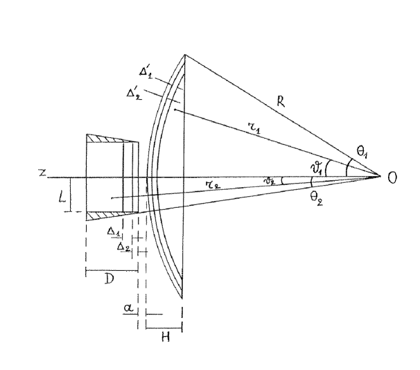
FIG. 1.: Configuration of a spherical lens and a disc. Point $O$ is the center of curvature of the lens with height $H$ and curvature radius $R$. The thickness of the disc is $D$ and its radius is $L$, $a$ being the distance between the disc and the lens. The thicknesses of $Cu$ and $Au$ layers on the lens are $\Delta_{1}^{\prime},\Delta_{2}^{\prime}$ and on the disc — $\Delta_{1},\Delta_{2}$ respectively. The small volume added to the disc in calculations is shown by hatching.

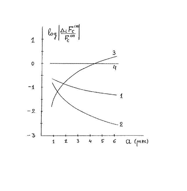
FIG. 2.: The relative role of different corrections to the Casimir force in configuration of a lens and a disc. Curve 1 shows the correction due to the finite conductivity ($\Delta_{\delta_{0}}F_{C}^{(0)}$), curve 2 shows the correction due to short-scale distortions ($\Delta_{d}F_{C}^{(0)}$), curve 3 shows the temperature correction ($\Delta_{T}F_{C}^{(0)}$). By the curve 4 the Casimir force itself is shown.

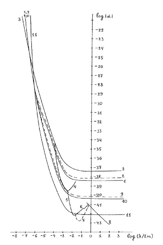
FIG. 3.: Constraints for the constants of hypothetical Yukawa-type interactions following from the force measurements. Curve 1 follows from the new measurement of the Casimir force ($\alpha>0$), curve 2 shows the same with $\alpha<0$, curve 3 results from the old Casimir force measurements between dielectric bodies [4]. Constraints from Cavendish-type experiments are shown by curve 4 [16], curve 5 [14], curve 6, $\alpha>0$ [14], curve 7, $\alpha<0$ [15]. Curve 8 follows from the Eötvös-type experiment [17]. Prospective constraints are shown by the curves 9–11: from the Casimir force measurements with iridium test bodies (curve 9, $\alpha>0$ and curve 10, $\alpha<0$), with iridium test bodies and the improved accuracy (curve 11). The regions of ($\lambda,\alpha$)-plane below the curves are permitted and above the curves are prohibited.

REFERENCES

• [1] H.B.G. Casimir, Proc. Kon. Nederl. Akad. Wet. 51, 793 (1948).
• [2] V.M. Mostepanenko and N.N. Trunov, The Casimir Effect and Its Applications (Clarendon Press, Oxford, 1997).
• [3] M.J. Sparnaay, Physica 24, 751 (1958).
• [4] B.V. Derjaguin, I.I. Abrikosova, and E.M. Lifshitz, Quart. Rev. 10, 295 (1956).
• [5] D. Tabor and R.H.S. Winterton, Proc. Roy. Soc. Lond. A 312, 435 (1969).
• [6] Y.N. Israelachvili and D. Tabor, Proc. Roy. Soc. Lond. A 331, 19 (1972).
• [7] S. Hunklinger, H. Geisselmann, and W. Arnold, Rev. Sci. Instr. 43, 584 (1972).
• [8] V.A. Kuz’min, I.I. Tkachev, and M.E. Shaposhnikov, JETP Letters (USA) 36, 59 (1982).
• [9] V.M. Mostepanenko and I.Yu. Sokolov, Phys. Lett. A 125, 405 (1987).
• [10] E. Fischbach et al, Metrologia 29, 215 (1992).
• [11] V.M. Mostepanenko and I.Yu. Sokolov, Phys. Lett. A 132, 313 (1988).
• [12] V.M. Mostepanenko and I.Yu. Sokolov, Phys. Rev. D 47, 2882 (1993).
• [13] M. Bordag, V.M. Mostepanenko, and I.Yu. Sokolov, Phys. Lett. A 187, 35 (1994).
• [14] J.K. Hoskins et al, Phys. Rev. D 32, 3084 (1985).
• [15] Y.T. Chen, A.H. Cook, and A.J.F. Metherell, Proc. Roy. Soc. Lond. A 394, 47 (1984).
• [16] V.P. Mitrofanov and O.I. Pononareva, Sov. Phys. JETP 67, 1963 (1988).
• [17] B.R. Heckel et al, Phys. Rev. Lett. 63, 2705 (1989).
• [18] G. Feinberg and J. Sucher, Phys. Rev. D 20, 1717 (1979).
• [19] V.M. Mostepanenko and I.Yu. Sokolov, Phys. Lett. A 146, 373 (1990).
• [20] S.K. Lamoreaux, Phys. Rev. Lett. 78, 5 (1997).
• [21] M. Bordag, G.T. Gillies, and V.M. Mostepanenko, Phys. Rev. D 56, R6 (1997); D 57, 2024 (1998).
• [22] G.L. Klimchitskaya, E.R. Bezerra de Mello, and V.M. Mostepanenko, Phys. Lett. A 236, 280 (1997).
• [23] G.L. Klimchitskaya and Yu.V. Pavlov, Int. J. Mod. Phys. A 11, 3723 (1996).
• [24] J. Blocki, J. Randrup, W.J. Swiatecki, and C.F. Tsang, Ann. Phys. (N.Y.) 115, 1 (1978).
• [25] V.M. Mostepanenko and I.Yu. Sokolov, Sov. Phys. Dokl. (USA) 33, 140 (1988).
• [26] M. Bordag, G.L. Klimchitskaya, and V.M. Mostepanenko, Int. J. Mod. Phys. A 10, 2661 (1995).
• [27] E.M. Lifshitz and L.P. Pitaevskii, Statistical Physics, Part 2, (Pergamon Press, Oxford, 1980).
• [28] V.B. Bezerra, G.L. Klimchitskaya, and C. Romero, Mod. Phys. Lett. A 12, 2613 (1997).
• [29] C.M. Hargreaves, Proc. Kon. Ned. Akad. Wet. B 68, 231 (1965).
• [30] J. Schwinger, L.L. DeRaad, and K.A. Milton, Ann. Phys. (N.Y.) 115, 1 (1978).
• [31] V.M. Mostepanenko and N.N. Trunov, Sov. J. Nucl. Phys. (USA) 42 812 (1985).
• [32] M. Bordag, G.L. Klimchitskaya, and V.M. Mostepanenko, Phys. Lett. A 20, 95 (1995).
• [33] L.S. Brown and G.J. Maclay, Phys. Rev. 184, 1272 (1969).
• [34] D.A. Varshalovich, A.N. Moskalev, and V.K. Khersonskii, Quantum Theory of Angular Momentum (World Scientific, Singapore, 1988).
• [35] I.S. Gradshteyn and I.M. Ryzhik, Table of Integrals, Series and Products (Academic, New York, 1980).
• [36] URL: http://www.netlib.org
• [37] S.K. Lamoreaux, Private communication.
• [38] V. Achilli, P. Baldi, G. Casula et al, Nuovo Cim. B 112, 775 (1997).
• [39] R. Onofrio and G. Carugno, Phys. Lett. A 198, 365 (1995).
Refer to caption