A new ${\cal O}(\alpha)$ correction to the decay rate of pionium

Abstract

Recently, much work has been devoted to the calculation of ${\cal O}(\alpha)$ corrections to the decay rate of pionium, the $\pi^{+}\pi^{-}$ bound state. In previous calculations, nonrelativistic QED corrections were neglected since they start at order $\alpha^{2}$ in hydrogen and positronium. In this note, we point out that there is one correction which is actually of order $\alpha$ times a function of the ratio $\mu_{r}\alpha/m_{e}$, where $\mu_{r}$ is the reduced mass of the system. When $\mu_{r}\alpha\ll m_{e}$, this function can be Taylor expanded and leads to higher order corrections. When $\mu_{r}\alpha\approx m_{e}$, as is the case in pionium, the function is of order one and the correction is of order $\alpha$. We use an effective field theory approach to calculate this correction and find it equal to $0.4298\,\alpha\Gamma_{0}$. We also calculate the corresponding contribution to the dimuonium ($\mu^{+}\mu^{-}$ bound state) decay rate and find a result in agreement with calculations by Jentschura et al.

I Introduction

The decay rate of pionium ($\pi^{+}\pi^{-}$ bound state) has generated much interest recently, because of the possibility of extracting from a future experiment at CERN [1] [2] precise values of the pion scattering lengths which can, in turn, be related to the quark condensate parameter, a fundamental ingredient of ChPT. In order to do so, however, all corrections of order $\alpha$ times the lowest order decay rate must be evaluated. These fall in several categories and have been the subject of several recent papers [3] [4] [5].

One can distinguish between pure QED corrections and corrections which arise from the interplay of strong and QED effects. The former are associated with an expansion in $\alpha$ whereas the latter contains an expansion in powers of $\alpha$ and other ChPT coefficients, such as scattering lengths, the pion mass difference, etc.

The pure QED corrections can be subdivided in relativistic and nonrelativistic contributions. This separation of scales is used, in one form or another, in all nonrelativistic bound state calculations but is the most transparent in the effective field theory (eft) formalism. The eft appropriate to the study of nonrelativistic QED bound states, NRQED, was developed by Caswell and Lepage more than ten years ago [6]. NRQED has since been used to calculate high order corrections to the hyperfine splitting of both muonium [7] and positronium [8]. Using NRQED, it is easy to convince oneself that in hydrogen and positronium, the ${\cal O}(\alpha)$ QED corrections are purely relativistic in nature whereas the nonrelativistic corrections start at order $\alpha^{2}$. This argument was used in [3] to dismiss the nonrelativistic corrections.

In this note, we want to point out that the vacuum polarization correction to the Coulomb interaction (referred to as the “VPC” correction in the following) is actually of order $\alpha$ times a function of the dimensionless ratio $\mu_{r}\alpha/m_{e}$, where $\mu_{r}$ is the reduced mass of the bound state. In hydrogen and positronium, this ratio is very small ($\approx\alpha$ and $\alpha/2$, respectively) and the function can be Taylor expanded, leading to a correction of higher order. In pionium, however, the ratio is equal to $0.997$ and the function turns out to be of order one. This means that the VPC correction represents an ${\cal O}(\alpha)$ correction to the lowest order rate. We want to emphasize that the observation that the VPC correction is enhanced in atoms with large reduced mass is not new; it is, for example, discussed in the Landau and Lifshitz textbook on quantum electrodynamics [9], in the context of energy levels.

Another system in which this type of correction is large is dimuonium, the $\mu^{+}\mu^{-}$ bound state. In that system, the ratio $\mu_{r}\alpha/m_{e}$ is about $0.754$ and the VPC correction is also of order $\alpha$ times the lowest order decay rate. This contribution was evaluated, among several other corrections, in a recent paper by Jentschura et al [10]. In this note, we use effective field theories to calculate the VPC contributions to both dimuonium and pionium. Our dimuonium result, $0.337\alpha\Gamma_{0}$, agrees with [10] Our result for pionium is equal to $0.430\,\alpha\Gamma_{0}$, which is as large as the other corrections evaluated in [3] [4].

We first consider the VPC corrections to the decay rate of dimuonium. For the present calculation, the only relevant interactions of the NRQED Lagrangian are

$${\cal L}_{fermions}~{} = {\psi^{\dagger}}\bigg{\{}i\partial_{t}+{\vec{D}^{2}\over 2m_{\mu}}-eA_{0})\biggr{\}}\psi~{}+~{}{\rm same~{}terms~{}with~{}}\psi\rightarrow\chi$$ (1)

$$- c_{4}~{}\psi^{\dagger}{\vec{\sigma}\,}\sigma_{2}\chi^{*}\,\cdot\,\chi^{T}\sigma_{2}{\vec{\sigma}\,}\psi-~{}c_{5}~{}\psi^{\dagger}\sigma_{2}\chi^{*}\,\cdot\,\chi^{T}\sigma_{2}\psi$$ (2)

where $\psi$ refers to the muon field, $\chi$ refers to the antimuon field and $m_{\mu}$ is the muon mass. Our sign convention for the coefficients $c_{4}$ and $c_{5}$ differs from [11] in order to avoid minus signs in the Feynman rules. To the order of interest, we can approximate the gauge derivative $\vec{D}$ by $\vec{p}$ since the correction due to transverse photons are suppressed (see [12]). The Feynman rules of the relevant interactions are presented in Fig.[1]. We work in Coulomb gauge in which the Coulomb photon propagator is simply given by $-1/\vec{k}^{2}$. The vacuum correction to the Coulomb propagator is also illustrated in Fig.[1]. We consider only the VPC because it is the only interaction which contributes at order $\alpha$ times a function of $\mu_{r}\alpha/m_{e}$. The vacuum polarization correction to the transverse propagator can be neglected because the vertices connecting transverse photons to fermions are suppressed by at least one power of the muon mass, which translates into additional factors of $\alpha$ in the bound state calculation (the interested reader is referred to [12] for more details on NRQED power counting rules).

The four-fermion operator proportional to $c_{4}$ leads to the decay rate of orthodimuonium (dimuonium with no angular momentum and a total spin equal to 1) whereas the other four-Fermi operator contributes to the decay of paradimuonium ($L=0,S=1$). In a nonrelativistic system, the Coulomb interaction is nonperturbative and must be summed up to all orders, which is equivalent to solving the Schrödinger equation. We will focus on the decay rate of the ground state ($n=1$), for which the wavefunction is given by

$$\Psi(\vec{p})={8\pi^{1/2}\gamma^{5/2}\over(\vec{p}^{2}+\gamma^{2})}\otimes\xi_{\mu^{+}}\otimes\xi_{\mu^{-}}$$ (3)

where the $\xi$’s are the two component Pauli spinors of the muon and antimuon and $\gamma\equiv\mu_{r}\alpha$ represents the typical bound state momentum (the ground state energy is given by $-\gamma^{2}/(2\mu_{r})$).

In NRQED, bound state properties are computed in two steps. First, one fixes the NQRED coefficients by matching QED and NRQED scattering amplitudes, and then one computes the bound state energy by applying time ordered perturbation theory to the NRQED vertices (with the Coulomb interaction defining the unperturbed problem). The decay rate is given in terms of the imaginary part of the energy by $\Gamma=$ -2 Im (E) .

To illustrate the use of NRQED, we now focus on the decay rate of orthodimuonium. To simplify the following discussion, we define the operator

$${\cal O}(\,^{3}S_{1})\equiv{\rm Im}(c_{4})\vec{S}^{2}$$ (4)

where the spectroscopic notation $\,{}^{2S+1}L_{J}$ is used to indicate the quantum numbers of a state annihilated by this operator. In terms of this operator, the decay rate is given by

$$\Gamma(1^{3}S_{1})=-2~{}{\langle{\Psi}|{{\cal O}(\,^{3}S_{1})}|{\Psi}\rangle}=-4|\Psi(\vec{r}=0)|^{2}{\rm Im}(c_{4})~{}=~{}-{m_{\mu}^{3}\alpha^{3}\over 2\pi}{\rm Im}(c_{4})$$ (5)

where a factor of 2 comes from the spin average of $\vec{S}^{2}$ and $|\Psi(\vec{r}=0)|^{2}=\gamma^{3}/\pi$. The imaginary part of the coefficient $c_{4}$ contains an infinite expansion in powers of $\alpha$, the lowest order contribution being found by performing the matching illustrated in Fig.[2]. All diagrams are computed exactly at threshold (no external momenta), in the center of mass frame of the particles, and a nonrelativistic normalization is used for the QED diagram (i.e. a factor of $1/\sqrt{2E}=1/\sqrt{2m}$ is provided for each external particle). Also, we match the amplitude matrix ${\cal M}$ and not $-i{\cal M}$. The superscript 1 on $c_{4}$ indicates that this is a contribution coming from a one-loop QED diagram. The NRQED diagram is simply $2\,{\rm Im}(c_{4}^{(1)})$ whereas the imaginary part of the QED diagram is $-2\pi\alpha^{2}/(3m_{\mu}^{2})$. Solving for the NRQED coefficient, we get

$${\rm Im}(c_{4}^{(1)})=-{\pi\alpha^{2}\over 3m_{\mu}^{2}}$$ (6)

which, after putting in Eq.(5) gives the lowest order rate,

$$\Gamma_{0}(1^{3}S_{1})={m_{\mu}\alpha^{5}\over 6}.$$ (7)

We now turn to the contribution from the vacuum polarization correction to the Coulomb photon. The first thing to do is to revise the matching of ${\rm Im}(c_{4})$ beyond one-loop. At first, this might seem unnecessary since we are interested in ${\cal O}(\alpha\Gamma_{0})$ corrections only, but we must be careful about factors of $m_{\mu}/m_{e}$ which might compensate for factors of $\alpha$. Indeed, this situation occurs in the matching illustrated in Fig.[3]. The result for the imaginary part of the QED diagram can be found from [13]:

$$2\times({\alpha\over\pi})^{2}\biggl{(}{9\zeta(2)\over 16}{m_{\mu}\over m_{e}}+{4\over 3}\ln({m_{\mu}\over m_{e}})+{22\over 36}+{\cal O}({m_{e}\over m_{\mu}})\biggr{)}\bigl{\{}-{2\pi\over 3}{\alpha^{2}\over m_{\mu}^{2}}\bigr{\}}$$ (8)

where the term in curly brackets is simply the lowest order result and the overall factor of 2 takes into account the two permutations of the diagram. The term proportional to $m_{\mu}/m_{e}$ represents a correction equal to $0.283\,\alpha$ and should therefore be treated as an ${\cal O}(\alpha)$ correction instead of an $\alpha^{2}$ correction. To the precision of interest in this work, we can neglect the log term, which comes from the running of the coupling constant, and all the other terms not enhanced by a factor of $m_{\mu}/m_{e}$. The calculation of the NRQED one-loop scattering diagram in Fig.[3] is straightforward:

$$\bigl{\{}-{2\pi\over 3}{\alpha^{2}\over m_{\mu}}\bigr{\}}~{}\int{d^{3}k\over(2\pi)^{3}}{-2\mu_{r}\over\vec{k}^{2}}~{}\int dv~{}{-4\alpha^{2}v^{2}(1-v^{2}/3)\over\vec{k}^{2}(1-v^{2})+4m_{e}^{2}}~{}=~{}{3\over 16}{m_{\mu}\over m_{e}}\alpha^{2}\bigl{\{}-{2\pi\over 3}{\alpha^{2}\over m_{\mu}^{2}}\bigr{\}}$$ (9)

which is seen to cancel exactly the $m_{\mu}/m_{e}$ term in the QED diagram. This is not a coincidence. The $m_{\mu}/m_{e}$ term is associated to the low energy behavior of the QED diagram, and since NRQED is designed to reproduce QED in the nonrelativistic limit, this term had to be present in the NRQED diagram. This will hold for higher order loop diagrams as well. The end result is that the coefficient ${\rm Im}(c_{4})$ does not receive any correction of order $\alpha(\alpha m_{\mu}/m_{e})^{n}\approx\alpha$ from the matching to QED. Therefore, we can simply use the lowest order coefficient ${\rm Im}(c_{4}^{(1)})$ given in Eq.(6) in the bound state calculation.

The bound state contribution of the VPC interaction is found by applying second order perturbation theory:

$$\delta\Gamma_{vpc}(\,^{3}S_{1})=2~{}\langle\,n\,|{\cal O}(\,^{3}S_{1})\sum_{m\neq n}\int{|\,m\,\rangle\,\langle\,m\,|\over E_{n}-E_{m}}\,V_{vpc}\,|\,n\,\rangle$$ (10)

where $V_{vpc}$ is the potential corresponding to the vacuum polarization correction to the Coulomb interaction:

$$V_{vpc}~{}=~{}\int_{0}^{1}dv{-4\alpha^{2}v^{2}(1-v^{2}/3)\over\vec{k}^{2}(1-v^{2})+4m_{e}^{2}}.$$ (11)

For the sum over intermediate states, we must include the full Coulomb Green’s function $G(\vec{p},\vec{q})$ in terms of which the previous expression can be written as

$$\delta\Gamma_{vpc}(\,^{3}S_{1})=-8\times \int{d^{3}p^{\prime}\over(2\pi)^{3}}{8\pi^{1/2}\gamma^{5/2}\over(\vec{p}^{\prime 2}+\gamma^{2})}{-\pi\alpha^{2}\over 3m_{\mu}^{2}}$$ (14)

$$\int{d^{3}p\,d^{3}q\,d^{3}k\over(2\pi)^{9}}~{}G(\vec{p},\vec{q})$$

$$~{}\biggl{(}\int_{0}^{1}dv{-4\alpha^{2}v^{2}(1-v^{2}/3)\over\vec{k}^{2}(1-v^{2})+4m_{e}^{2}}\biggr{)}{8\pi^{1/2}\gamma^{5/2}\over(\vec{p}-\vec{k})^{2}+\gamma^{2}}$$

$$=2\int{d^{3}p\,d^{3}q\,d^{3}k\over(2\pi)^{9}}~{}G(\vec{p},\vec{q})~{}\biggl{(}\int_{0}^{1}dv{-4\alpha^{2}v^{2}(1-v^{2}/3)\over\vec{k}^{2}(1-v^{2})+4m_{e}^{2}}\biggr{)}{8\pi\gamma\over(\vec{p}-\vec{k})^{2}+\gamma^{2}}~{}\Gamma_{0}$$ (15)

where, in the first expression, a factor of -2 comes from the relation $\Gamma=-2$ Im(E), a factor of 2 comes from the spin average, and another one comes from the two sides on which the interaction can take place. The second expression gives the correction in terms of the lowest order rate, $\Gamma_{0}$. For the Coulomb Green’s function, we use the following expression derived by Schwinger [14]:

$$G(\vec{p},\vec{q})~{}=~{}-{2\mu_{r}\over\vec{p}^{2}+\gamma^{2}}(2\pi)^{3}\delta^{3}(\vec{q})-{16\pi\mu_{r}^{2}\alpha\over(\vec{p}^{2}+\gamma^{2})(\vec{p}-\vec{q})^{2}(\vec{q}^{2}+\gamma^{2})}-{64\pi\over\alpha\gamma^{4}}R(\vec{p},\vec{q})$$ (16)

where the first term corresponds to no Coulomb interaction in the intermediate state, the second term corresponds to one Coulomb line and the third term corresponds to the the exchange of two or more Coulomb photons. We will refer to these three terms as the $0-C$, $1-C$ and $R$ contributions, respectively. A graphical representation of Eq.(15) is presented in Fig.[4]. An explicit expression for $R(\vec{p},\vec{q})$ can be found in [14]. All we need for the present work is the following integral [15]

$$\int(d^{3}pd^{3}q)f(p)R(\vec{p},\vec{q})~{}=~{}-4\pi^{3}\gamma^{7}~{}\int_{0}^{\infty}\,dp~{}{p^{2}\,f(p)\over(\vec{p}^{2}+\gamma^{2})^{2}}\biggl{(}\ln(2)-{5\over 2}+{\gamma\over p}{\rm Arctan}({p\over\gamma})-{1\over 2}\ln(1+{\vec{p}^{2}\over\gamma^{2}})+{4\gamma^{2}\over\vec{p}^{2}+\gamma^{2}}\biggr{)}$$ (17)

where $f(p)$ is an arbitary function of the magnitude of the three-momentum $\vec{p}$.

We now calculate the correction to the decay rate of orthodimuonium. The no Coulomb correction to Eq.(15) can be integrated analytically and is found to be

$$\Delta E_{0-C}~{}=~{}{2\over\pi^{3}}\,I_{0}(r)~{}\alpha\Gamma_{0}$$ (18)

where $I_{0}$ is a function of the dimensionless ratio $r\equiv\gamma/m_{e}=\mu_{r}\alpha/m_{e}$ which is $0.754$ in dimuonium. For the sake of completeness, we give $I_{0}(r)$ for arbitrary values of r:

$$I_{0} = \pi^{2}\biggl{(}-{5\over 9}-{1\over 3r^{2}}+{\pi\over r}\bigl{(}{1\over 4}+{1\over 6r^{2}}\bigr{)}+{\bigl{(}-2r+1/r+1/r^{3}\bigr{)}\over 3{\sqrt{1-r^{2}}}}\biggl{\{}{\rm ArcTan}\bigl{(}{r\over{\sqrt{1-r^{2}}}}\bigr{)}-{\pi\over 2}\biggr{\}}\biggr{)}~{}~{}~{}(r<1)$$ (19)

$$= {\pi^{2}\over 36}\bigl{(}-32+15\pi\bigr{)}~{}~{}~{}(r=1)$$ (20)

$$= \pi^{2}\biggl{(}-{5\over 9}-{1\over 3r^{2}}+{\pi\over r}\bigl{(}{1\over 4}+{1\over 6r^{2}}\bigr{)}-{\bigl{(}-2r+1/r+1/r^{3}\bigr{)}\over 6{\sqrt{r^{2}-1}}}\biggl{\{}{\rm ln}\bigl{(}{{\sqrt{r^{2}-1}}+r\over r-{\sqrt{r^{2}-1}}}\bigr{)}\biggr{\}}\biggr{)}~{}~{}~{}(r>1).$$ (21)

Using Eq.(18) with $r=0.754$, the no Coulomb contribution to the dimuonium decay rate is found to be

$$\Delta E_{0-C}({\rm dimuonium})~{}=~{}0.216\alpha\Gamma_{0}~{}~{}.$$ (22)

We have reduced the one Coulomb and R term contributions of Eq.(15) to two dimensional integrals (using the identity (17)) which were evaluated using the adaptive Monte-Carlo integration routine Vegas [16]. The results are respectively

$$\Delta E_{1-C}({\rm dimuonium})~{}=~{}0.08674\,\alpha\Gamma_{0}$$ (23)

$$\Delta E_{R}({\rm dimuonium})~{}=~{}0.0344\,\alpha\Gamma_{0}$$ (24)

leading to a total equal to (sum of Eqs.(18), (23) and (24)) $0.337\alpha\Gamma_{0}$. This result agrees with Ref.[10] which gives $(1.06/\pi)\alpha\Gamma_{0}=0.337\alpha\Gamma_{0}$. Notice that the lowest order decay rate of paradimuonium is also given in terms of a four-Fermi interaction (the interaction proportional to $c_{5}$ in the Lagrangian) so that the VPC correction is also $0.337\,\alpha\Gamma_{0}$ where $\Gamma_{0}$ is now the lowest order paradimuonium decay rate.

The calculation of the VPC correction to the pionium decay rate is very similar to the dimuonium calculation. This is the most apparent by using a nonrelativistic field theory reproducing ChPT at low energy, which we will refer to as “NRChPT”. The only NRChPT interactions relevant to the present calculation are the Coulomb interaction (for the charged pions) and the four-pion vertex of the form $\pi^{+}\pi^{-}\pi^{0}\pi^{0}$ (a more detailed presentation of NRChPT and calculations of the other ${\cal O}(\alpha)$ corrections will be presented elsewhere).

The matching of the four pions interaction is presented in Fig.[5]. At threshold, the ChPT amplitude for the $\pi^{+}\pi^{-}\pi^{0}\pi^{0}$ vertex is equal to $32\pi(a_{0}^{0}-a_{0}^{2})/3$, where $a_{0}^{i}$ is the scattering amplitude in the isospin channel $i$. Using a nonrelativistic normalization for the external states, we divide by a factor

$$({\sqrt{2E_{\pi^{0}}}})^{2}{\sqrt{2E_{\pi^{+}}}}{\sqrt{2E_{\pi^{-}}}}\approx 4m_{\pi^{0}}m_{\pi^{+}}\approx 4m_{\pi^{+}}^{2}$$ (25)

where we have set $\Delta m_{\pi}\equiv m_{\pi^{+}}-m_{\pi^{0}}=0$. As we will see below, this is possible because we are interested in the decay reate to leading order in $\Delta m_{\pi}$ (the ${\cal O}(\Delta m_{\pi})$ corrections will be treated in a future publication). The end result of the matching is that the coefficient of the NRChPT four-pion interaction is

$$C_{4-pions}~{}=~{}{8\pi\over 3}{(a_{0}^{0}-a_{0}^{2})\over m_{\pi^{+}}^{2}}.$$ (26)

For the coulomb photon and the VPC interaction, we use the same Feynman rules as in the dimuonium calculation. As before, the Coulomb interaction must be summed up to all orders, which means that the $\pi^{+}\pi^{-}$ state will be described by the same ground state Schrödinger wavefunction as before. The lowest order rate is trivially computed by considering the NRChPT interaction sandwiched between wavefunctions:

$$\Delta{\rm E}~{}=~{}{1\over 2}\int{d^{3}p\over(2\pi)^{3}}\Psi(\vec{p})~{}C_{4pions}\int{d^{3}q\over(2\pi)^{3}}~{}G_{\pi^{0}\pi^{0}}(\vec{q}^{2})~{}C_{4pions}\int{d^{3}p^{\prime}\over(2\pi)^{3}}\Psi(\vec{p}^{\prime})$$ (27)

where the overall factor of $1/2$ is a symmetry factor and $G_{\pi^{0}\pi^{0}}(\vec{q}^{2})$ is the free propagator of the $\pi^{0}\pi^{0}$ pair, given by

$$G_{\pi^{0}\pi^{0}}(\vec{q}^{2})={1\over E_{0}-E_{intermediate}}\approx{1\over 2m_{\pi^{+}}-2m_{\pi^{0}}-\vec{q}^{2}/m_{\pi^{0}}+i\epsilon}$$ (28)

where we have neglected the binding energy in $E_{0}$ (the full expression is $E_{0}=2m_{\pi^{+}}(1-\alpha^{2}/8)$) since it leads to a correction of order $\alpha^{2}\Gamma_{0}$. The difference $2m_{\pi^{+}}-2m_{\pi^{0}}=2\Delta m_{\pi}$ appearing in Eq.(28) cannot be set to zero since it leads to the imaginary part of the integral and, therefore, to the first order decay rate. A trivial integration gives, for the integral Eq.(27)

$$\Delta E~{}=~{}-|\Psi(0)|^{2}{16m_{\pi^{0}}\over 9}{(a_{0}^{0}-a_{0}^{2})^{2}\over m_{\pi^{+}}^{4}}\bigl{(}\Lambda+i{\pi\over 2}{\sqrt{m_{\pi^{0}}}}{\sqrt{2\Delta m_{\pi}}}\bigr{)}$$ (29)

where $\Lambda$ is an ultraviolet cutoff on the $|\vec{q}|$ integration which would be canceled by a counterterm in a calculation of the bound state energy [17]. Since we are only interested in the decay rate, we need only to concentrate on the imaginary part of the energy. Working in first order in $\Delta m_{\pi}$, Eq.(29) finally leads to a decay rate equal to the well-known result

$$\Gamma_{0}=-2{\rm Im}(E)={16\pi\over 9}{\sqrt{2\Delta m_{\pi}\over m_{\pi^{+}}}}{(a_{0}^{0}-a_{0}^{2})^{2}\over m_{\pi^{+}}^{2}}~{}|\Psi(0)|^{2}.$$ (30)

Turning now to the VPC correction, we have to carry out the integral given in Eq.(15), using the reduced mass of pionium, $\mu_{r}=m_{\pi^{+}}/2$. The no-Coulomb term is clearly given by Eq.(18), with $r=m_{\pi^{+}}\alpha/(2m_{e})\approx 0.997$. We find a result equal to

$$\Delta E_{0-C}({\rm pionium})~{}=~{}0.26677\,\alpha\Gamma_{0}.$$ (31)

We have also computed the one Coulomb and R term contributions to the pionium decay rate using VEGAS and found

$$\Delta E_{1-C}({\rm pionium})~{}=~{}0.1193\,\alpha\Gamma_{0}~{}$$ (32)

$$\Delta E_{R}({\rm pionium})~{}=~{}0.04372\,\alpha\Gamma_{0}.$$ (33)

Our final result is the sum of Eqs.(31), (32) and (33):

$$\Delta E_{vpc}({\rm pionium})~{}=~{}0.4298\,\alpha\Gamma_{0}$$ (34)

which is of the same order of magnitude as the other corrections calculated in [3] and [4].

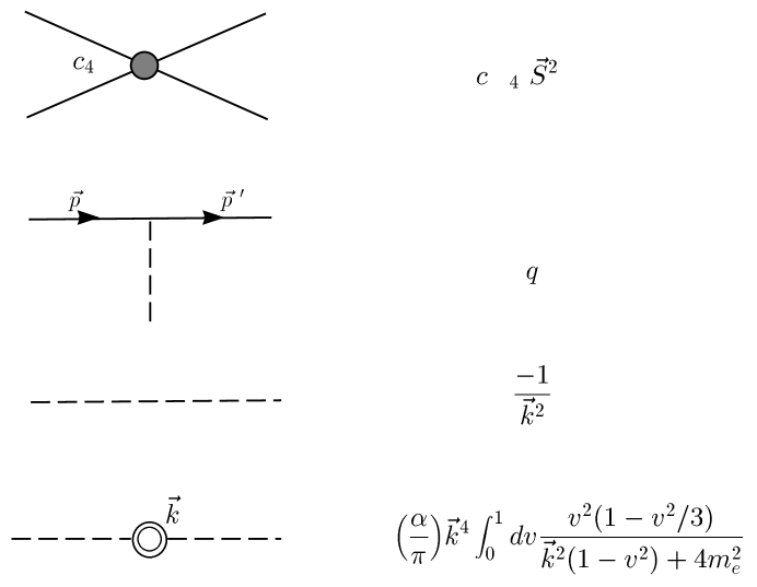
FIG. 1.: NRQED Feynman rules (q represents the charge of the particle). The last three rules can also be applied to NRChPT.

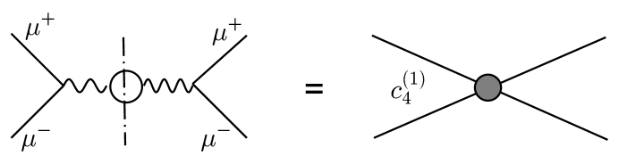
FIG. 2.: Lowest order matching of ${\rm Im}(c_{4})$ (the imaginary part is implicit in the figure).

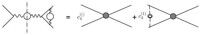
FIG. 3.: Vacuum polarization correction to the coefficient ${\rm Im}(c_{4})$ (the imaginary part of the coefficients is implicit in the figures).

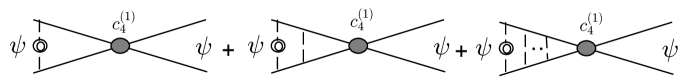
FIG. 4.: VPC correction to the dimuonium decay rate. The three diagrams represent the no Coulomb, one Coulomb and R contributions (the imaginary part of the coefficients is implicit in the figures).

FIG. 5.: Lowest order matching of the ChPT and NRChPT $\pi^{+}\pi^{-}\pi^{0}\pi^{0}$ interaction.

- [1] G. Czapek et al, letter of intent, CERN/SPSLC 92-44.
- [2] L.L. Nemenov, Sov. J. Nucl. Phys. 41, 629 (1985).
- [3] H. Jallouli and H. Sazdjan, preprint hep-ph/9706450.
- [4] V.E. Lyubovitskij, E.Z. Lipartia and A.G. Rusetskii, Pisma Zh.Eksp.Teor.Fiz. 66, 747 (1997); JETP Lett. 66, 783 (1997).
- [5] M. Knecht and R. Urech, preprint hep-ph/9709348.
- [6] W.E. Caswell and G.P. Lepage, Phys. Lett. B167, 437 (1985).
- [7] M. Nio and T. Kinoshita, Phys. Rev. D53, 4909 (1996); Phys. Rev. D55, 7267 (1997).
- [8] A.H. Hoang, P. Labelle and S.M. Zerbarjad, Phys. Rev. Lett. 79, 3387 (1997).
- [9] V.B. Berestetskii, E.M. Lifshitz and L.P. Pitaevskii, Landau and Lifshitz Course of Theoretical Physics, Quantum Electrodynamics, Pergamon Press, 1980.
- [10] U.D. Jentschura, G. Soff, V.G. Ivanov and S.G. Karshenboǐm, hep-ph/9706026.
- [11] P. Labelle, S.M. Zebarjad and C. Burgess, Phys. Rev. D56, 8053 (1997).
- [12] P. Labelle, preprint hep-ph/9608491.
- [13] A.H. Hoang, Karlsruhe University PhD thesis, Dec. 1995.
- [14] J. Schwinger, J. Math. Phys., 5, 1606 (1964).
- [15] W.E. Caswell and G.P. Lepage, Phys. Rev. A18, 810 (1978).
- [16] G.P. Lepage, J. Comput. Phys. 27, 192 (1978).
- [17] P. Labelle, Cornell University PhD thesis, UMI-94-16736-mc (microfiche), Jan. 1994.