Abstract

We investigate the critical behaviour of a three-dimensional lattice $\chi U\phi_{3}$ model in the chiral limit. The model consists of a staggered fermion field, a $U(1)$ gauge field (with coupling parameter $\beta$) and a complex scalar field (with hopping parameter $\kappa$). Two different methods are used: 1) fits of the chiral condensate and the mass of the neutral unconfined composite fermion to an equation of state and 2) finite size scaling investigations of the Lee-Yang zeros of the partition function in the complex fermion mass plane. For strong gauge coupling ($\beta<1$) the critical exponents for the chiral phase transition are determined. We find strong indications that the chiral phase transition is in one universality class in this $\beta$ interval: that of the three-dimensional Gross-Neveu model with two fermions. Thus the continuum limit of the $\chi U\phi_{3}$ model defines here a nonperturbatively renormalizable gauge theory with dynamical mass generation. At weak gauge coupling and small $\kappa$, we explore a region in which the mass in the neutral fermion channel is large but the chiral condensate on finite lattices very small. If it does not vanish in the infinite volume limit, then a continuum limit with massive unconfined fermion might be possible in this region, too.

PACS numbers: 11.15.Ha, 11.30.Qc, 12.60.Rc, 11.10.Kk

${}^{*})$ UKQCD Collaboration

1 Introduction

Strongly coupled gauge theories are interesting candidates for new mass generating mechanisms because they tend to break chiral symmetry dynamically. However, the fermions which acquire mass through this mechanism usually get confined. It was pointed out [1] that this can be avoided in a class of chiral symmetric strongly coupled gauge theories on the lattice in which the gauge charge of the fermion is shielded by a scalar field of the same charge. The question is, whether these models are nonperturbatively renormalizable at strong gauge coupling such that the lattice cutoff can be removed. If so, the resulting theory might be applicable in continuum and constitute a possible alternative to the Higgs mechanism [1].

In this work we investigate such a lattice model in three dimensions with a vectorlike U(1) gauge symmetry, which we call $\chi U\phi_{3}$ model. It consists of a staggered fermion field $\chi$ with a global U(1) chiral symmetry, a gauge field $U\in\mbox{U(1)}$ living on the lattice links of length $a$ and a complex scalar field $\phi$ with frozen length $|\phi|=1$. It is characterized by the dimensionless gauge coupling parameter $\beta$ (proportional to the inverse squared coupling constant), the hopping parameter $\kappa$ of the scalar field and the bare fermion mass $am_{0}$. The unconfined fermion is the composite state $F=\phi^{\dagger}\chi$. In a phase with broken chiral symmetry, it has nonvanishing mass $am_{F}$ in the chiral limit $m_{0}=0$. The $\chi U\phi_{3}$ model can be seen either as a generalization of three-dimensional compact QED with a charged scalar field added or as three-dimensional U(1) Higgs model with added fermions.

The same model has also been investigated in two and four dimensions. In two dimensions it seems to be in the universality class of the Gross-Neveu model [2] at least for strong gauge coupling, thus being renormalizable. Therefore the shielded gauge-charge mechanism of dynamical mass generation suggested in [1] works in two dimensions and its long range behaviour is equivalent to the four fermion theory. In four dimensions there is also a region in $\beta$ ($0\leq\beta<0.64$) in which the model behaves in a very similar manner to the corresponding four-fermion theory, the Nambu–Jona-Lasinio model with a massive fermion whose mass scales at the critical point [3]. Here both models belong to the same universality class and have the same renormalizability properties. But for intermediate coupling there evidently exists a special point. It is a tricritical point at which, together with the composite fermion $F$, scaling of a particular scalar state was found. This composite scalar can be interpreted as a gauge ball mixing with a $\phi^{\dagger}$-$\phi$ state. Thus the gauge degrees of freedom play an important dynamical role and the model belongs to a new universality class of models with dynamical mass generation, whose renormalizability is of much interest [4, 5].

In this paper we investigate the phase diagram and the critical behaviour of the model in three dimensions. We find that in the chiral limit $m_{0}=0$ the $\chi U\phi_{3}$ model has three regions in the $\beta-\kappa$ plane with different properties with respect to the chiral symmetry. They are indicated in Fig. 1. The region at strong gauge coupling (small $\beta$) and small $\kappa$ is the Nambu phase where the chiral symmetry is broken and the neutral fermion $F$ is massive. At large $\kappa$ chiral symmetry is restored and the fermion $F$ is massless. This phase is labelled the Higgs phase because of its properties in the weak coupling limit. The third is the X region at large $\beta$ and small $\kappa$. It is conceivable that this region is analytically connected with either the Nambu or Higgs phase but it may well be a separate phase. In this region the mass measured in the fermion channel is large, but the chiral condensate is very small (within our numerical accuracy consistent with zero).

Figure 1: Phase diagram of the $\chi U\phi_{3}$ model for $m_{0}=0$. For $\beta<1$ a clear phase transition between the Nambu and Higgs phases can be observed. Whether the region X at large $\beta$ and small $\kappa$ forms a third phase or belongs to one of the other phases, separated from it only by a crossover, is discussed in the text. All phase transitions seem to be 2^nd order.

The main result of our paper is the determination of the critical behaviour at strong gauge coupling. We find strong indications that the chiral phase transition between the Nambu and Higgs phases is in one universality class for all $\beta\lesssim 1$. It is the class of the three-dimensional Gross-Neveu model which is known to be (nonpertubatively) renormalizable [6]. That model is the $\beta=0$ limit of the $\chi U\phi_{3}$ model [7]. This universality means that the continuum limit of the $\chi U\phi_{3}$ model defines a nonperturbatively renormalisable gauge theory in which the fermion mass is generated dynamically by the shielded gauge-charge mechanism. However, it also means that in this $\beta$ region the gauge field is auxiliary and the $\chi U\phi_{3}$ model does not represent a new class of field theories.

The chiral properties of the region X are elusive and their determination would require substantial effort and resources. This is beyond the scope of the present work and we made only an exploratory investigation. But we point out that, provided the chiral symmetry is broken there, the phase transition between the region X and the Higgs phase gives rise to another possible construction for a continuum theory containing an unconfined fermion with dynamically generated mass. It could continue to be in the universality class of the three-dimensional Gross-Neveu model. But experience [4, 5] with the four-dimensional model in the vicinity of the tricritical point suggests that at larger $\beta$ the gauge degrees of freedom are dynamical and a new universality class may be present. This interesting possibility, and the possible existence of a tricritical point in three dimensions, deserves further study.

Our investigation is mainly based on two methods: firstly, via fits to an equation of state and, secondly, via a finite size scaling investigation of the Lee-Yang zeros in the complex fermion mass plane. The investigation of a phase transition via fits to an equation of state is quite reliable because the finite size effects we find close to the phase transition are usually small. Therefore we expect a simple finite size scaling, describe it by an empirical formula and extrapolate observables to the infinite volume. Then we do a simultaneous fit to the fermion mass $am_{F}$ and the chiral condensate $\langle\overline{\chi}\chi\rangle$.

As first pointed out by Lee and Yang [8, 9], the determination of the finite size scaling behaviour of the complex zeros of a partition function could be a direct method for the determination of the critical properties of the associated theory. In this paper we investigate these zeros of the canonical partition function in the complex bare fermion mass plane. These zeros control the fermion condensate and its associated susceptibilities [10, 11], physical quantities which are often measured directly on the lattice and used, via finite size scaling, to determine the critical behaviour.

In the region X, where the chiral condensate is very small, both methods fail to provide reliable results. A small condensate suggests that the Lee-Yang zeros cannot be near to the physical region. Nevertheless, it is of interest to investigate if the closest zeros can be determined with sufficient accuracy to ascertain their finite size scaling (and hence that of the condensate).

The paper is organized as follows. In the next section we introduce the model in detail, define the observables we use and briefly summarize the method of the Lee-Yang zeros. In section 3 we present evidence for the universality at strong gauge coupling. In section 4 we present the results obtained at weak coupling and discuss their possible interpretations. In the last section our results are summarized.

2 The model

The $\chi U\phi_{3}$ model is defined on a 3-dimensional cubic lattice with periodic boundary conditions except for antiperiodic boundary conditions for the fermion field in the “time” direction. The action reads:

$$S_{\chi U\phi}=S_{\chi}+S_{U}+S_{\phi},$$ (1)

with

$$S_{\chi} = \frac{1}{2}\sum_{x}\overline{\chi}_{x}\sum_{\mu=1}^{3}\eta_{\mu x}(U_{x,\mu}\chi_{x+\mu}-U^{\dagger}_{x-\mu,\mu}\chi_{x-\mu})+am_{0}\sum_{x}\overline{\chi}_{x}\chi_{x}\;,$$

$$S_{U} = \beta\sum_{x,\mu<\nu}(1-{\rm Re}\,{U_{x,\mu\nu}})\;,$$

$$S_{\phi} = -\kappa\sum_{x}\sum_{\mu=1}^{3}(\phi^{\dagger}_{x}U_{x,\mu}\phi_{x+\mu}+{\rm h.\,c.})\;.$$

Here $\chi_{x}$ are the Kogut-Susskind fermion fields with $\eta_{\mu x}=(-1)^{x_{1}+\cdots+x_{\mu-1}}$. Because of doubling our model describes two four-component fermions ($N_{f}=2$). The bare mass $am_{0}$ of the fermion is introduced for technical reasons. We are interested in the chiral limit $m_{0}=0$. The $a$ in front of $m_{0}$ indicates that we have to distinguish between the chiral limit in the continuum ($m_{0}=0$) and the continuum limit of the lattice model, where $am_{0}\rightarrow 0$ can also be achieved by $a\rightarrow 0$ at nonzero $m_{0}$.

$U_{x,\mu}$ represents the compact link variable and $U_{x,\mu\nu}$ is the plaquette product of the link variables $U_{x,\mu}$.

The hopping parameter $\kappa$ vanishes, if the square of the bare mass of the scalar field is $+\infty$, and is infinite if the bare mass squared is $-\infty$. The scalar field $\phi$ has frozen length $|\phi|=1$. This choice is made in order to restrict the number of parameters of the model. Without that, symmetries and dimensionality of couplings would allow several other terms in the action.

We stress that the charges of the fundamental fields exclude a direct Yukawa coupling between the fundamental fields.

The model has some interesting limiting cases. For $\kappa=0$ the scalar field decouples and the model is equivalent to three-dimensional compact QED with fermions. It is known [12, 13, 14, 15] that pure compact QED has no phase transition and, as $\beta\rightarrow\infty$, it is confining via a linear potential with an exponentially decreasing string tension. There is an indication that, with fermions, chiral symmetry is broken at large coupling, but at weak coupling results are inconclusive [16]. It has been suggested that, in noncompact QED with fermions, the phase diagram is dependent on the number of flavors and that, at weak coupling, chiral symmetry is broken only for a small number (less than about 3.5) of fermions [17, 18, 19, 20]. (A recent description of the status of three-dimensional QED can be found in [21, 22].) It is quite probable that, at weak coupling, both the compact and non-compact formulations have quite similar properties. If so, then these (uncertain) features suggest that the chiral symmetry is broken in the $\kappa=0$ limit of the phase X and thus presumably in the whole phase X.

In the weak gauge coupling limit, $\beta=\infty$, the fermions are free with mass $am_{0}$, and $S_{\phi}$ reduces to the XY₃ model. It has a phase transition at $\kappa\approx 0.27$.

At $am_{0}=\infty$ the model reduces to the three-dimensional compact U(1) Higgs model. For its recent investigation with numerous references see [23].

For $\beta=0$ the gauge and scalar fields can be integrated out exactly [7] and one ends up with a lattice version of the three-dimensional four-fermion model

$$S_{4f}=-\sum_{x}\sum_{\mu=1}^{3}[G\overline{\chi}_{x}\chi_{x}\overline{\chi}_{x+\mu}\chi_{x+\mu}-\frac{1}{2}\eta_{\mu x}(\overline{\chi}_{x}\chi_{x+\mu}-\overline{\chi}_{x+\mu}\chi_{x})]+\frac{am_{0}}{r}\sum_{x}\overline{\chi}_{x}\chi_{x},$$ (2)

the parameters $G$ and $r$ being related to $\kappa$ [7, 1].

We refer to this model as the Gross-Neveu model. Some caution is in place, however. There is some uncertainty whether the four-fermion model (2) is a lattice version of the Gross-Neveu model or of the Thirring model. The four-fermion action (2) was used in four dimensions for the study of the Nambu–Jona-Lasinio model e.g. in [24, 25], which would correspond to the Gross-Neveu model in three dimensions. Recently in [26, 27] the four-fermion action (2) in three dimensions is interpreted as the Thirring model and similar interpretation is implied by K.-I. Kondo [28]. For our number of fermions, $N_{f}=2$, the distinction might be unimportant and both models might actually coincide. The Gross-Neveu model has a chiral phase transition and is nonperturbatively renormalisable (see [6, 29] and references therein). The properties of the $N_{f}=2$ Thirring model appear to be similar [28, 26, 27]. For our purposes the important property of the three-dimensional four-fermion model obtained in the $\beta=0$ limit of the $\chi U\phi_{3}$ model is its renormalisability, which presumably holds for both interpretations.

2.1 Observables

Because we are interested in the chiral properties of the model we concentrate on the chiral condensate and the fermion mass.

The chiral condensate is defined by

$$\langle\overline{\chi}\chi\rangle=\left\langle{\rm Tr}\,M^{-1}\right\rangle$$ (3)

where $M$ is the fermion matrix. The trace is measured with a gaussian estimator.

The physical fermion of the $\chi U\phi_{3}$ model is the gauge invariant composite fermion $F=\phi^{\dagger}\chi$. We measure its mass $am_{F}$ in momentum space with the usual procedure, as described (for the model in 4 dimensions) in [3]. We checked that the results are in good agreement with the fits done in configuration space. In the three-dimensional model we find the fits to $G^{1\!\!1}$ to be the most stable, so we use them for the data shown in this paper.

Both observables need to be extrapolated to infinite volume. This procedure is described in section 3.1.

We remark that the required numerical effort for the study of the $\chi U\phi_{3}$ model was very high. We needed significantly more matrix inversions than for the four-dimensional case [5] at the same volume and $am_{0}$. Their number also depends significantly on $\beta$: The simulation at $\beta=0$ required about O(1000) conjugate-gradient steps, about 2-5 times more than at larger $\beta$-values. Surprisingly, the number of required steps scattered in a very broad interval. The maximal step-number was at least a factor of 2-3 above the average. This might be connected with the observation, that the chiral condensate has a very asymmetric distribution.

2.2 Equation of State

A standard way to analyse the critical exponents of a chiral phase transition is via the use of an equation of state (EOS). Normally data close to the phase transition can be well described by such an ansatz. In our model for fixed $\beta$ this equation reads

$$am_{0}=\langle\overline{\chi}\chi\rangle^{\delta}F\left((\kappa-\kappa_{c})\langle\overline{\chi}\chi\rangle^{-1/\beta_{\chi}}\right)\;,\quad F(x)=Rx+S\,.$$ (4)

Here $\langle\overline{\chi}\chi\rangle$ is the infinite volume value of the chiral condensate for given $am_{0}$, $\kappa$ and $\beta$. $\beta_{\chi}$ and $\delta$ are the exponents defined in analogy to a magnetic transition. The index $\chi$ is added to distinguish the exponent and the coupling. The scaling function $F$ is used in its linear approximation and $R$ and $S$ are free constants. We apply this equation in the region for which $\kappa\approx\kappa_{c}$ and where we might expect the scaling deviations to be small.

It is also useful to assume the corresponding scaling equation for the fermion mass:

$$am_{0}=(am_{F})^{1/\tilde{\nu}}G\left((\kappa-\kappa_{c})(am_{F})^{-1/\nu}\right)\;,\quad G(x)=Ax+B\,.$$ (5)

The exponent $\nu$ is the correlation length critical exponent in the chiral plane ($am_{0}=0$). $\tilde{\nu}$ is an analogous exponent obtained if one approaches the critical point from outside the chiral plane. The two exponents have to be distinguished. At fixed $\beta$ in the chiral plane ($am_{0}=0$) the fermion mass scales with $\nu$: $am_{F}\propto(\kappa-\kappa_{c})^{\nu}|_{am_{0}=0}$, whereas for all other straight paths into the critical point (for example $\kappa=\kappa_{c}$) it scales with $am_{0}$ as: $am_{F}\propto{am_{0}}^{\tilde{\nu}}|_{\kappa-\kappa_{c}\propto am_{0}}$. This is indicated in figure 2 in the plane $\beta=const$.

Figure 2 also illustrates that for $\kappa<\kappa_{c}$ the chiral condensate changes sign and makes a jump if one crosses the line $am_{0}=0$. This means that it is a line of first order phase transitions. For $\kappa>\kappa_{c}$ the line becomes a line of second order phase transitions on which the fermion mass gets critical. In between there is a critical point ($\kappa=\kappa_{c}$).

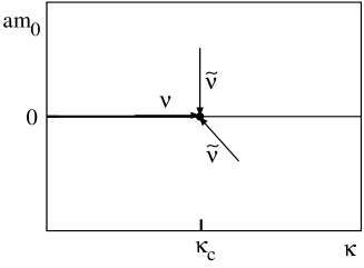
Figure 2: First order chiral phase transition line (bold line) and the critical point in a plane $\beta=const$. The fermion mass $am_{F}$ scales with exponent $\nu$ in the direction tangential to the transition line and with exponent $\tilde{\nu}$ in any other direction.

If hyperscaling holds, only two of the four exponents defined by the equations of state are independent. The corresponding scaling relations are:

$$\delta=\frac{1}{d\tilde{\nu}-1}\quad\mbox{and}\quad\beta_{\chi}=\nu\left(d-\frac{1}{\tilde{\nu}}\right)\,,$$ (6)

where $d=3$ is the space-time dimension.

2.3 Lee-Yang zeros

The canonical partition function, after integration over the Grassmann variables and using the irrelevance of overall multiplicative factors, can be defined as:

$$Z(\beta,\kappa,am_{0})=\frac{\int dUd\phi\det M[am_{0},U]e^{S_{U\phi}}}{\int dUd\phi\det M[a\hat{m}_{0},U]e^{S_{U\phi}}}.$$ (7)

Here $S_{U\phi}=S_{U}+S_{\phi}$, $M$ is the usual fermionic matrix for Kogut-Susskind fermions and $a\hat{m}_{0}$ is some (arbitrary) “updating” fermion mass at which the ensemble of gauge fields is generated.

Since the mass dependence of $M$ is purely diagonal, the partition function can be written as the average over the ensemble of the characteristic polynomials of $M$, i. e.:

$$Z(\beta,\kappa,am_{0}) = \left\langle\frac{\sum_{n=0}^{V\over 2}C_{n}[U[\beta,\kappa]](am_{0})^{2n}}{\det M[a\hat{m}_{0},U[\beta,\kappa]]}\right\rangle_{a\hat{m}_{0}}$$ (8)

$$= \sum_{n=0}^{V\over 2}A_{n}[\beta,\kappa](am_{0})^{2n}.$$ (9)

The coefficients $C_{n}$ of the characteristic polynomial are obtained from the eigenvalues of $M[0,U]$ which are imaginary and appear in complex conjugate pairs. In the simulations described below they were obtained using the Lanczos algorithm.

The Lee-Yang zeros are the zeros of this polynomial representation of the partition function. The zeros were found by using a standard root finding algorithm on the equivalent sets of polynomials generated as in Eq. ($8$):

$$\sum_{n=0}^{V\over 2}A_{n}^{i}(am_{0}^{2}-a\bar{m}_{i}^{2})^{n}$$ (10)

for a set of $a\bar{m}_{i}$ in the region where we expect the lowest zeros to occur. This allowed us to avoid the problems associated with rounding errors in the root-finder. We required that a zero be found consistently for the subset of the $a\bar{m}_{i}$ closest to it. These zeros in the bare mass we label as $y_{i}$ in the following.

The errors in the Lee-Yang zeros are estimated by a Jacknife method. The coefficents for each lattice size were averaged to produce $6$ subsets of averaged coefficients, each taking into account $5/6$ of the measurements. These $6$ different sets of coefficients give $6$ different results for the Lee-Yang zeros from which the variance was calculated.

The critical properties of the system are determined by the zeros lying closest to the real axis. The zero with the smallest imaginary part we label $y_{1}$. It is also called edge singularity. With increasing finite volume it converges to the critical point. For a continuous phase transition the position of the zeros closest to the real axis in the complex plane is ruled by the scaling law

$$y_{i}(\beta,\kappa,L)-y_{R}(\beta,\kappa,\infty)=A_{i}L^{-1/s},$$ (11)

where the $A_{i}$’s are complex numbers. The exponent $s=s(\beta,\kappa)$ describes the finite size scaling of the correlation length. For our model $y_{R}(\beta,\kappa,\infty)=0$ and we ignore it in the following.

It immediately follows that the real and the imaginary parts of the zeros should scale independently with the same exponent. In particular, for the zero $y_{1}$ closest to the chiral phase transition (at $am_{0}=0$)

$${\rm Im}\,y_{1}(\beta,\kappa,L)=A_{I}L^{-1/s},$$ (12)

with a similar scaling behaviour for ${\rm Re}\,y_{1}(\beta,\kappa,L)$ via $A_{R}$. In practice the real part of the zero is much smaller than its imaginary part or is identically zero. So eq. (12) usually provides a more reliable measure of the exponent than the scaling of the real part.

Although the above scaling law was originally established for the case of a continuous phase transition, it can also be extended to that of a first order phase transition. Since there is no divergent correlation length, the exponent is determined only by the actual dimension of the system. In this case, for a three-dimensional model we expect $s=\frac{1}{3}$.

At the critical point ($\kappa=\kappa_{c}$) we expect $s$ to be equal to $\tilde{\nu}$, because the fermion correlation length should be the relevant one. In the symmetric phase ($\kappa>\kappa_{c}$) we expect scaling with $s=1$, because $am_{F}\propto am_{0}$. This behaviour is indicated in Fig. 3 by the full lines and the dot.

Figure 3: Schematic plot of the exponent $s$ in infinite volume (full lines and dot) and the effective $s$ in finite volume (dashed line).

Figure 4: Expected finite size scaling of the zero $y_{1}$ with lattice size.

In practice it is important to understand the scaling deviations on a finite lattice. The expected behaviour is shown schematically in Fig. 4. Far away from the critical point we expect linear scaling in the log-log plot with $s=1/3$ in the broken phase, and $s=1$ in the symmetric phase. At the critical point we expect linear scaling and the exponent should be $s=\tilde{\nu}$. These expectations are indicated by the full lines. Close to the phase transition, we expect a crossover. For small lattice sizes the exponent should be close to $\tilde{\nu}$ and then change to $1/3$ and $1$, respectively, if the lattice size is increased and the true scaling shows up. This is indicated in Fig. 4 by the dashed lines. For a set of lattice sizes this defines an effective $s$ which smoothly goes through $\tilde{\nu}$ at the critical point. Such an effective $s$ is represented in Fig. 3 by a dashed line.

Therefore, in order that the critical exponent can be determined, we must either know the position of the critical point accurately or have many simulations on large lattices so that the scaling deviations can be measured accurately. In practice the limited knowledge of the position of the critical point leads to the largest uncertainty in the determination of $\tilde{\nu}$ by this method.

3 Universality at Strong Coupling

At strong coupling the chiral phase transition can be seen clearly and we investigate the scaling behaviour and the universality along this line.

We determined the Lee-Yang zeros, the chiral condensate and the fermion mass for various values of $\kappa$ at $\beta=0.00$ and 0.80. In this section we want to investigate how the transition changes as $\beta$ increases from zero. Therefore we have investigated the scaling of the data at $\beta=0$, i.e. the four-fermion model, as a reference and compare it with the scaling found at $\beta=0.80$.

3.1 Equation of State

Here we determine the critical exponents of the chiral phase transition by using the EOS for $am_{F}$ and $\langle\overline{\chi}\chi\rangle$. Although we did simulations on lattices up to $24^{3}$, our conclusions still depend to some extent on our choice of ansatz for the extrapolation of $am_{F}$ and $\langle\overline{\chi}\chi\rangle$ to infinite volume. Fig. 5 shows, as an example, our data for $am_{F}$ at $\beta=0.80$ and $am_{0}=0.01$ plotted against $1/L^{2}$.

Figure 5: Data for $am_{F}$ at $\beta=0.80$ and $am_{0}=0.01$ plotted against $1/L^{2}$. The dotted lines are a fit with eq. (13) to the data with $L\geq 16$.

For the extrapolation we tried three approaches:

$$am_{F}(L) = am_{F}(\infty)+A\frac{1}{L^{2}}\,,$$ (13)

$$am_{F}(L) = am_{F}(\infty)+A\frac{1}{L}\,,$$ (14)

$$am_{F}(L) = am_{F}(\infty)+A\frac{1}{L}\exp(-am_{F}(\infty)\,L)\,.$$ (15)

Each has two free parameters: $am_{F}(\infty)$ and $A$. To judge the quality of the fits we first compared the $\chi^{2}$ per degree of freedom using our data on $16^{3}$, $20^{3}$ and $24^{3}$ lattices. This was done at the values of $\beta$ and $\kappa$ at which we have good statistics. Our results are shown in table 1. It turned out that the results for these lattice sizes are not conclusive as to which extrapolation formula should be used, because, for each ansatz, all $\chi^{2}$ per degree of freedom are usually below 1.

			Fit 1		Fit 2		Fit 3
$\beta$	$\kappa$	$am_{0}$	$am_{F}$	$\chi^{2}$	$am_{F}$	$\chi^{2}$	$am_{F}$	$\chi^{2}$
0.00	0.95	0.01	0.269(3)	0.30	0.256(7)	0.53	0.278(2)	0.01
0.00	1.00	0.01	0.194(4)	0.22	0.180(9)	0.45	0.202(2)	0.01
0.00	1.05	0.01	0.132(5)	0.23	0.111(10)	0.04	0.142(3)	0.62
0.00	0.95	0.02	0.337(3)	0.41	0.327(6)	0.22	0.343(1)	2.07
0.80	0.40	0.01	0.441(8)	0.12	0.437(2)	0.15	0.445(3)	0.03
0.80	0.42	0.01	0.276(8)	0.01	0.247(16)	0.08	0.295(4)	0.31
0.80	0.43	0.01	0.215(5)	0.07	0.191(9)	0.01	0.230(2)	1.33
0.80	0.45	0.01	0.122(2)	0.01	0.087(1)	0.14	0.137(3)	0.36

Table 1: Results of the fits to the finite size behaviour at different couplings and masses on $16^{3}$, $20^{3}$, $24^{3}$ lattices. The extrapolated infinite volume mass $am_{F}=am_{F}(\infty)$ and the $\chi^{2}$ per degree of freedom for the three fits are given: with eq. (13) (Fit 1), eq. (14) (Fit 2) and eq. (15) (Fit 3).

However, the fit with eq. (13) is significantly prefered if compared with the $12^{3}$ data. We therefore adopted this fit for our extrapolations, but data from the $12^{3}$ lattice was not included. Such an extrapolation is indicated in Fig. 5 by the dotted lines.

For the chiral condensate the finite size effects are in general smaller and with opposite sign. Again, consideration of the $12^{3}$ lattices favoured a fit ansatz analogous to eq. (13).

We describe in detail the analysis in which we used the ansatz of eq. (13) to extrapolate all our data for $am_{F}$ and $\langle\overline{\chi}\chi\rangle$, obtained on $16^{3}$ and larger lattices, to infinite volume. The error was calculated with the MINOS routine from the MINUIT library. All results presented in the following change somewhat quantitatively, but not qualitatively, if a different extrapolation formula is used.

The data at different $\kappa$ and $am_{0}$, extrapolated to the infinite volume, were analyzed by means of the EOS. We included only the data at $am_{0}=0.01$ and $am_{0}=0.02$. The chosen $\kappa$ range was 0.80 … 1.05 for $\beta=0.00$ and 0.38 … 0.47 for $\beta=0.80$.

As a first step we analyzed the data for $am_{F}$ and $\langle\overline{\chi}\chi\rangle$ independently and fitted to their corresponding EOS (5) and (4). The results are given in table 2. As can be seen, for both $\beta$’s the critical $\kappa$ values $\kappa_{c}$ are identical within the error bars.

	$\beta$	$\kappa_{c}$	$\nu$	$\tilde{\nu}$	$A$	$B$	$\chi^{2}$
$am_{F}$:	0.00	0.987(33)	0.91(22)	0.43(8)	1.1(3)	0.38(8)	0.72
	0.80	0.425(5)	0.78(14)	0.40(5)	3.6(6)	0.33(5)	0.82
	$\beta$	$\kappa_{c}$	$\beta_{\chi}$	$\delta$	$R$	$S$	$\chi^{2}$
$\langle\overline{\chi}\chi\rangle$:	0.00	0.983(12)	0.56(5)	3.1(3)	1.3(2)	1.1(3)	0.84
	0.80	0.429(7)	0.56(10)	3.0(5)	4.4(12)	2.4(13)	0.58

Table 2: Results of fits at $\beta=0.00$ and 0.80 using the equations of state. The upper table shows the results of the fit of $am_{F}$ based on eq. (5), the lower table those of $\langle\overline{\chi}\chi\rangle$ based on eq. (4).

As a next step we performed a simultaneous fit with one common $\kappa_{c}$ for $am_{F}$ and $\langle\overline{\chi}\chi\rangle$ (table 3). A very good fit to all the data was obtained.

Then we checked the scaling relations (6). Calculating $\beta$ and $\delta$ with $\nu$ and $\tilde{\nu}$ gives $\beta_{\chi}=0.54(20)$ and $\delta=3.8(15)$ for $\beta=0.00$ and $\beta_{\chi}=0.39(25)$ and $\delta=5(3)$ for $\beta=0.80$. The agreement with the fit is quite good. Note that in (6), $d\tilde{\nu}=3\tilde{\nu}$ is close to 1 and hence the statistical errors are increased.

$\beta$	$\kappa_{c}$	$\nu$	$\tilde{\nu}$	$\beta_{\chi}$	$\delta$	$\chi^{2}$
0.00	0.983(12)	0.88(8)	0.42(3)	0.56(5)	3.1(3)	0.71
0.80	0.425(4)	0.78(11)	0.40(4)	0.47(5)	3.4(3)	0.71

Table 3: Results of fits of $am_{F}$ and $\langle\overline{\chi}\chi\rangle$ at $\beta=0.00$ and 0.80, using both equations of state with a common $\kappa_{c}$.

We also tried a third fit in which we assumed the validity of the scaling relations (6). The result is shown in Figs. 7 and 7 and summarized in table 4. As one can see, the quality of the fit is still good and $\chi^{2}$ are reasonable. The figures also show the prediction of our fit for the fermion mass and chiral condensate at $am_{0}=0.04$ and 0.06. Only small deviations are visible. We therefore conclude that (6) is consistent with our data.

$\beta$	$\kappa_{c}$	$\nu$	$\tilde{\nu}$	$\chi^{2}$	$\beta_{\chi}$	$\delta$
0.00	0.981(6)	0.79(2)	0.437(5)	2.2	0.56(4)	3.2(2)
0.80	0.425(2)	0.75(2)	0.431(6)	2.3	0.51(4)	3.4(2)

Table 4: Results of our fits using the equations of state at $\beta=0.00$ and 0.80 with one $\kappa_{c}$ and the scaling relations (6) at $\beta=0.00$ and 0.80.

Figure 6: (a) Fermion mass and (b) chiral condensate for $\beta=0.00$. The data are our extrapolation into the infinite volume. The fit assumes the validity of the scaling relations and is described in the text. The parameters are given in table 4. The dashed line shows the extrapolation into the chiral limit.

Figure 7: (a) Fermion mass and (b) chiral condensate for $\beta=0.80$.

The values of the exponents $\nu$, $\tilde{\nu}$, and $\beta_{\chi}$ in table 2 and table 3 agree with those in table 4. Thus all three fitting procedures gave consistent results at each $\beta$.

Furthermore, the exponents obtained at $\beta=0.00$ and $\beta=0.80$ agree within errors. This is a strong signal that the chiral phase transition is in one universality class at these $\beta$’s and probably also for those in between. The difference in the exponents of the last fit, which is somewhat larger than the pure statistical errors may for example be the result of small scaling deviations.

To estimate the uncertainty due to the choice of the extrapolation formula, we repeated the above procedures using the extrapolation (14). The results are given in table 5. The $\chi^{2}$’s are even smaller and the exponents differ by a little more than one standard deviation. Although the agreement for the two $\beta$’s is less good, it is still compatible with universality if one takes into account that the error bars only reflect the statistical errors and not the uncertainty due to scaling deviations.

$\beta$	$\kappa_{c}$	$\nu$	$\tilde{\nu}$	$\chi^{2}$	$\beta_{\chi}$	$\delta$
0.00	0.968(9)	0.76(3)	0.426(8)	0.89	0.50(6)	3.6(3)
0.80	0.419(3)	0.66(4)	0.409(10)	0.64	0.37(6)	4.4(6)

Table 5: Results of fits, when we use eq. (14) for the extrapolation to infinite volume. As in table 4, the equations of state with common $\kappa_{c}$ and the scaling relations (6) are used.

3.2 The Finite Size Scaling of the Lee-Yang Zeros

The Lee-Yang zeros were found to be purely imaginary at all values of $\kappa$ in the strong coupling region. For small $\kappa$ they are equally spaced, consistent with a strong first order transition in the condensate as the bare mass $am_{0}$ goes through zero.

Figs. 8 and 9 show the finite size scaling behaviour of the edge singularity at various $\kappa$ for $\beta=0.00$ and $0.80$, respectively. Our data confirm the expectations presented in section 2.3 and Fig. 4. Close to the critical point we see the expected crossover: for small lattices the exponent is close to $\tilde{\nu}$ and shifts for increasing lattice size to the exponent $1/3$ or $1$.

Figure 8: Imaginary part of zero $y_{1}$ as function of the lattice size for different $\kappa$ at $\beta=0.00$. The different straight lines should help to investigate the linearity and claim only for $\kappa=0.975\approx\kappa_{c}$ (full line) to describe the data well.

Figure 9: Imaginary part of zero $y_{1}$ as function of the lattice size for different $\kappa$ at $\beta=0.80$.

At small $\kappa$ the exponent $s$ is consistent with a first order phase transition, $s\lower 3.01385pt\hbox{$\;\stackrel{{\scriptstyle\textstyle>}}{{\sim}}\;$}\frac{1}{3}$. At large $\kappa$ is $s\lesssim 1$. Close to the critical point, determined in the previous section and given in table 4, the data scale linearly on the log-log plot allowing determination of $\tilde{\nu}$.

At the $\kappa$ points closest to $\kappa_{c}$ we expect $s\simeq\tilde{\nu}$. At $\beta=0.00$ we find at $\kappa=0.975\simeq\kappa_{c}=0.981(6)$ the exponent $s=0.440(4)$ in excellent agreement with $\tilde{\nu}=0.437(5)$, as determined in the previous section. For $\beta=0.80$ we did the simulations at $\kappa=0.43$ slightly larger than the $\kappa_{c}=0.425(2)$ obtained from the EOS. Not unexpectedly we found $s=0.447(5)$, slightly larger than $\tilde{\nu}=0.431(6)$ from the EOS. This shows the great importance of the knowledge of the critical point for a precision measurement of $\tilde{\nu}$. Within these uncertainties the agreement is very good and again confirms the independence of $\tilde{\nu}$ from $\beta$ and hence the universality.

If one analyses these plots without the knowledge of the critical point determined with the EOS, the critical point can also be determined by looking for linearity of $\ln[Im(y_{1})]$ as a function of $\ln L$. For this purpose we show in Figs. 10 and 11 the quantity $\ln[Im(y_{1})]+1/\tilde{\nu}\ln L$. The addition of the second term makes the plots approximately horizontal and so allows us to enhance the vertical scale making the error bars clearer. In the figures we have used $\tilde{\nu}=0.440$ and $0.501$, respectively. The dashed lines are a linear extrapolation of the data points at the two lowest $L$-values. They provide a guide as to the linearity of the data.

Figure 10: $\ln[Im(y_{1})]+1/\tilde{\nu}\ln L$ with $\tilde{\nu}=0.440$ as a function of the lattice size for different $\kappa$’s at $\beta=0.00$. The dashed straight lines are linear extrapolations to the data points at the lowest two values of $L$.

Figure 11: As in the previous figure but at $\beta=0.80$ with $\tilde{\nu}=0.501$.

Figs. 10 and 11 suggest a larger $\kappa_{c}$ and $s(\kappa_{c})$ than those obtained from the EOS analysis. For example, at $\beta=0.80$, Fig. 11 would suggest $\kappa=0.45$ as the point closest to $\kappa_{c}$, with $\tilde{\nu}\simeq s(0.45)=0.501(6)$. However, the difference between the two methods of analysis is about 10% which is the same size as the statistical error.

All in all, this demonstrates the reliability of the methods we have used. Both (very different) methods agree rather well and their combination is very useful.

3.3 Universality at strong coupling

Our data are a good indication that the chiral phase transition of the $\chi U\phi_{3}$ model is in the same universality class at $\beta=0.00$ and $\beta=0.80$. Assuming this universality we combine the results for exponents at both $\beta$ values and determine the exponents of this chiral phase transition to be $\nu=0.75(10)$ and $\tilde{\nu}=0.43(2)$. The errors take into account the uncertainties discussed above. These values of $\nu$ and $\tilde{\nu}$ correspond to $\beta_{\chi}=0.51(11)$ and $\delta=3.45(71)$. We note that the position of the critical point at $\beta=0$, as well as the results for $\delta$ and $\beta$ are compatible with those obtained for the $N_{f}=2$ case in [27] ($\beta_{\chi}=0.57(2)$ and $\delta=2.75(9)$). In that work the same action (2) has been simulated, though in a somewhat different representation by means of auxiliary fields than the $\beta=0$ limit of the $\chi U\phi_{3}$ model.

It is very likely that the chiral phase transition is in the same universality class for $\beta$ between 0 and the onset of the X region around $\beta\simeq 1$. The universality might be expected at small $\beta$ because of the convergence of the strong coupling expansion. But our data are (to our knowledge) the first indication that this is true for a large $\beta$ interval.

This result indicates that the $\chi U\phi_{3}$ model is renormalizable in this region of $\beta$. So it is a nontrivial example in three dimensions for the shielded gauge-charge mechanism of fermion mass generation proposed in [1].

We note that, in the scaling investigation, the chiral condensate, which is a pure fermionic operator, and the mass of the fermion $F$, which is a combination of the fermion and the scalar field, have been used. Both seem to scale in a way which can be well described by the usual scaling relations.

The universality on the other hand also means that, with respect to the three-dimensional Gross-Neveu model, nothing substantially new happens at small and intermediate $\beta$ and no new physics arises on scales much below the cutoff. The scalar field shields the fermion $\chi$ giving rise to the fermion $F$ equivalent to the fermion of the four-fermion theory. We find no indication that composite states consisting only of fundamental scalars or gauge fields, which would not fit into the Gross-Neveu model, scale at the chiral phase transition.

The bosonic fields appear to be auxiliary at strong gauge coupling, as they are in a rigorous sense [7] at $\beta=0$. As indicated by the results in four dimensions [4, 5], this may change as the gauge coupling gets weaker. We therefore performed some studies at larger values of $\beta$. The results are described in the next section.

4 Explorative study of the weak coupling region

4.1 Condensate and fermion mass

We should point out again that the compact three-dimensional QED with fermions is not fully understood at large $\beta$. It is not clear, at large $\beta$, if there is chiral symmetry breaking and confinement via a linear potential. This uncertainty extends also to our model with $\kappa$ small. A clarification of these difficult questions would require a substantial effort far beyond the scope of this paper. Thus our aim is to perform an explorative study only and to get some insight into this as yet unexplored region. Also we want to see how far the methods applied successfully at strong coupling can be of use also at weaker coupling. The physical interpretation of our results will leave room for several scenarios.

Fig. 12 shows the fermion mass and condensate at $\kappa=0.25$ as a function of $\beta$, at three values of the bare fermion mass.

Figure 12: (a) fermion mass and (b) chiral condensate for different small $am_{0}$ as function of $\beta$ at $\kappa=0.25$ on the $8^{2}16$ lattice.

The neutral fermion mass decreases for increaing $\beta$ but then stabilizes with $am_{F}>1$. So it is clearly nonzero at all $\beta$ and again only weakly dependent on the bare fermion mass. The condensate is large at small $\beta$ (the Nambu phase) but rapidly decreases with $\beta$ and becomes very small (zero?) in the chiral limit for $\beta>\beta_{X}\simeq 1.3$. Thus here a new, weakly coupled region is encountered.

In order to see how this region is related to the Higgs phase at large $\kappa$, the fermion mass and condensate are shown in Fig. 13 at $\beta=2.0$ and three values of the bare fermion mass. For nonvanishing bare mass, where the simulations have been performed, the mass of the neutral fermion is large for $\kappa<\kappa_{X}\simeq 0.27$ whereas it is small for larger $\kappa$. It is only very weakly dependent on the bare fermion mass and therefore we expect this behaviour to persist in the chiral limit. For $\kappa>\kappa_{X}$ its small nonzero value probably vanishes in the infinite lattice size limit.

The condensate, as expected, does depend strongly on the bare mass $am_{0}$ but does show a crossover behaviour at $\kappa=\kappa_{X}$ with $\langle\overline{\chi}\chi\rangle(am_{0})_{\kappa<\kappa_{X}}<\langle\overline{\chi}\chi\rangle(am_{0})_{\kappa>\kappa_{X}}$. However, at large $\kappa$ we believe that we are in the Higgs phase where the condensate is zero in the chiral limit. It is therefore conceivable that, in this limit, it is zero at $\beta=2.0$ for all $\kappa$. It is very surprising, however, that, at fixed bare fermion mass and lattice size, the condensate tends to slightly increase with increasing $\kappa$, quite in contrast from its behaviour in the strong coupling region. Of course, this can change in the infinite volume and chiral limit.

Figure 13: (a) fermion mass and (b) chiral condensate for different small $am_{0}$ as function of $\kappa$ at $\beta=2.00$ on the $8^{2}16$ lattice.

At the coupling $\kappa=\kappa_{X}$, where the fermion mass shows a possible crossover behaviour, there is also a peak in the susceptibility of the link energy which increases with increasing lattice volume. However, a careful finite size scaling analysis would be needed to determine if it indicates a phase transition or a crossover.

Fig. 14a confirms the weak dependence of the fermion mass $am_{F}$ on the bare mass. At $\kappa=0.22$ below $\kappa_{X}$, the fermion mass is large and stays clearly nonzero at $am_{0}$. Above $\kappa_{X}$, at $\kappa=0.34$, the fermion mass is too small for the lattice size used and might vanish in the infinite volume limit.

Figure 14: (a) Fermion mass and (b) chiral condensate for different $\kappa$ as function of $am_{0}$ at $\beta=2.00$ on the $8^{2}16$ lattice.

Fig. 14b shows that, at $\beta=2.0$ and $\kappa$ just below or above $\kappa_{X}$, the condensate extrapolates linearly in $am_{0}$ to a very small value or zero. As we shall see below, this is due to the Lee-Yang edge singularity in this region being relatively distant from the real axis.

A naive extrapolation to the chiral limit would thus classify the region at small $\kappa$ ($\kappa<\kappa_{X}$) and large $\beta$ ($\beta>\beta_{X}$) as a phase with zero chiral condensate and nonvanishing fermion mass. But the condensate could also remain very small but nonvanishing. Because of this uncertainty we label this region X. Its boundaries $\beta_{X}$ and $\kappa_{X}$ may slightly depend on $\kappa$ and $\beta$, respectively.

It would be surprising if in the region X the fermion mass was different from zero with unbroken chiral symmetry. There are essentially two scenarios avoiding such a paradox.

1) Chiral symmetry breaking persists at small $\kappa$ also for $\beta>\beta_{X}$. $\chi$ is light, because the chiral condensate is very small, though nonzero. $F$ is a bound state of $\phi$ and $\chi$. The binding might be quite loose, presumably by a weak linear confining potential, which one expects in pure U(1) in 3d [13, 14, 15]. $F$ is heavy essentially because $\phi$ is heavy. The transition at $\beta=\beta_{X}$ is probably a cross-over, but a genuine phase transition is not excluded.

In this scenario the region X must be separated by a chiral phase transition at $\kappa_{X}(\beta)$ from the Higgs phase. As our data around $\kappa_{X}$ do not indicate any metastability, it would be a higher order transition and a continuum limit should be possible. Thus an interesting continuum limit with massive unconfined fermion might exist.

2) Chiral symmetry is restored at $\beta=\beta_{X}$ and the chiral condensate thus vanishes identically and $\chi$ is massless in X. The $F$ channel gets contribution from the two-particle state $\phi$ and $\chi$. This contribution appears as a massive state because $\phi$ is heavy. This state presumably cannot be a bound state in the chiral limit because of the old argument of Banks and Casher [30]: fermion on a closed orbit must be able to flip its helicity, i.e. existence of the bound state implies chiral symmetry breaking. We cannot distinguish between a bound state $F$ and a two-particle state $\phi$ + $\chi$ looking at the $F$ channel only (as we did). X could be connected to the Higgs phase, where we expect the same spectrum.

Which of these scenarios is true might be investigated in the limit case $\kappa=0$, i.e. in the three-dimensional compact QED. The results in the noncompact case [17, 18, 19, 20] might be applicable at weak coupling also to the compact one. As the number of fermions in our case is below the critical number $\simeq 3.5$ of fermions in the noncompact model, the more interesting scenario 1) seems to be preferred.

4.2 The Lee-Yang zeros at Weak Coupling

In an attempt to clarify the situation at weak coupling we have also investigated the Lee-Yang zeros in the region X. The edge singularity $y_{1}$ has a nonzero real part in this region. The finite size scaling of the lowest zeros is shown in Fig. 15 for $\beta=2.00$, $\kappa=0.15$, a point in the middle of the region X. The real part of the low lying zeros is clearly nonvanishing. Then the first two zeros have within the numerical precision identical imaginary part but their real parts differ by a factor of about 3.5.

The first two zeros have imaginary parts so close as to be indistinguishable within statistical error. We have assumed continuity in the behaviour of their real parts as a function of lattice size when plotting Fig. 15.

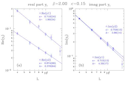
Figure 15: (a) Real and (b) imaginary part of the first two Lee Yang zeros (sorted by their positive imaginary part) for $\beta=2.00$, $\kappa=0.15$ as function of lattice size.

These imaginary parts scale linearly in the log-log plot with an exponent $s=0.73(4)$ where the error is given by the difference between the two zeros. Their real part has somewhat larger errors but scales within the numerical precision with the same exponent. This pattern for the edge singularity is found throughout the region X. Note that this behaviour is only observed in the edge singularity.

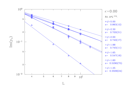
Figure 16: Imaginary part of zero $y_{1}$ as function of the lattice size for different $\beta$ at $\kappa=0$.

Fig. 16 shows the behaviour of the imaginary part of the edge as a function of lattice size at $\kappa=0$ for various $\beta$. There is a crossover between $\beta=1.25$ and $\beta=1.88$, i. e. from the Nambu phase, where the imaginary part of the edge zero is small and the transition first order, to a region where the imaginary part is large (with nonzero real part) again consistent with a vanishing condensate. No scaling deviations can be observed for $\beta\geq 1.88$. In the region X the critical exponent has a very weak dependence on $\beta$ and increases only very slowly on further increase of $\kappa$.

If the scaling in the region X is different from that in the other regions, the most naive expectation would be that the exponent $s$ is universal. This is compatible with our data at $\beta\approx 2$ but not at $\beta=5$. Further simulations on larger lattice are necessary to confirm this difference.

It is to our knowledge the first model in which scaling of the real part of the edge singularity to zero has been observed. We do not understand the implications of this behaviour. It may well be a key point in understanding the critical nature of region X.

Summarizing, the region X can be distinguished from the Nambu and Higgs phase by the edge singularity having a real part (on a finite lattice) and a scaling which cannot be described by either an exponent $s=1/3$ or $s=1$. If the exponent $s$ is different from those in Nambu and Higgs phases then the region X is presumably a new phase. We have been unable to determine if the chiral symmetry is broken or not in this region.

5 Conclusions

We have presented an extensive analysis of the phase structure of the three-dimensional fermion-gauge-scalar model. The analysis has been made possible by the application of two different methods: $1$)fits to an equation of state of the chiral condensate and the mass of the physical neutral fermion and $2$)finite size scaling investigations of the Lee-Yang zeros of the partition function in the complex fermion mass plane.

Our investigations showed that there are three regions in the $\beta$-$\kappa$ plane with possibly different critical behaviour in the chiral limit:

a) The region at small $\kappa$ and strong gauge coupling, where the chiral symmetry is broken and the neutral physical fermion is massive, called the Nambu phase.

b) The region at large $\kappa$, where the chiral symmetry is restored and the physical fermion is massless, called the Higgs phase.

c) A third region at weak coupling and small $\kappa$, where the chiral condensate is zero within our numerical accuracy but the neutral fermion mass is large, called the X region. This region can analytically be connected with either the Nambu or Higgs phase but it may well be a separate phase. If chiral symmetry is not broken in this region, then the mass observed in the fermion channel is presumably the energy of a two-particle state. Otherwise this region might be an interesting example of dynamical mass generation of unconfined fermions. If the continuum limit is taken at the Higgs phase transition, the gauge fields should play an important dynamical role and the model would not fall into the universality class of the three-dimensional Gross-Neveu model. A further investigation of this possibility is highly desirable.

At strong gauge coupling, the chiral phase transition can be clearly localized, and there are strong indications that it is in one universality class for all $\beta<1$: that of the three-dimensional Gross-Neveu model, which is known to be non-pertubatively renormalizable. This demonstrates that the three-dimensional lattice $\chi U\phi_{3}$ model is a nonperturbatively renormalizable quantum field theory and the shielded gauge-charge mechanism of fermion mass generation [1] works in three dimensions.

Acknowledgements

We thank M. Göckeler, S. J. Hands, and K.-I. Kondo for discussions, and J. Paul for valuable contributions in the early stage of this work. The computations have been performed on the Fujitsu computers at RWTH Aachen, and on the CRAY-YMP and T90 of HLRZ Jülich. E.F., W.F., and J.J. acknowledge the hospitality of HLRZ.

The work was supported in part by DFG. I.B. was supported in part by the TMR-network ”Finite temperature phase transitions in particle physics”, EU-contract ERBFMRX-CT97-0122.

References

- [1] C. Frick and J. Jersák, Phys. Rev. D52 (1995) 340.
- [2] W. Franzki, J. Jersák, and R. Welters, Phys. Rev. D54 (1996) 7741.
- [3] W. Franzki, C. Frick, J. Jersák, and X. Q. Luo, Nucl. Phys. B453 (1995) 355.
- [4] W. Franzki and J. Jersák, Strongly coupled U(1) lattice gauge theory as a microscopic model of Yukawa theory, PITHA 97/42, HLRZ1997_65, hep-lat/9711038, submitted to Phys. Rev. D.
- [5] W. Franzki and J. Jersák, Dynamical fermion mass generation at a tricritical point in strongly coupled U(1) lattice gauge theory, PITHA 97/43, HLRZ1997_66, hep-lat/9711039, to appear in Phys. Rev. D.
- [6] B. Rosenstein, B. J. Warr, and S. H. Park, Phys. Rev. Lett. 62 (1989) 1433.
- [7] I.-H. Lee and R. E. Shrock, Phys. Rev. Lett. 59 (1987) 14.
- [8] C. N. Yang and T. D. Lee, Phys. Rev. 87 (1952) 410.
- [9] T. D. Lee and C. N. Yang, Phys. Rev. 87 (1952) 410.
- [10] I. M. Barbour, A. J. Bell, and E. G. Klepfish, Nucl. Phys. B389 (1993) 285.
- [11] I. M. Barbour, R. Burioni, and G. Salina, Phys. Lett. 341B (1995) 355.
- [12] A. M. Polyakov, Phys. Lett. 59B (1975) 82.
- [13] A. M. Polyakov, Nucl. Phys. B120 (1977) 429.
- [14] T. Banks, R. Myerson, and J. Kogut, Nucl. Phys. B129 (1977) 493.
- [15] M. Göpfert and G. Mack, Commun. Math. Phys. 82 (1982) 545.
- [16] A. N. Burkitt and A. C. Irving, Nucl. Phys. B295 [FS21] (1988) 525.
- [17] T. Appelquist, D. Nash, and L. C. R. Wijewardhana, Phys. Rev. Lett. 60 (1988) 2575.
- [18] E. Dagotto, J. B. Kogut, and A. Kocic, Phys. Rev. Lett. 62 (1989) 1083.
- [19] E. Dagotto, J. B. Kogut, and A. Kocic, Nucl. Phys. B334 (1990) 279.
- [20] S. Hands and J. B. Kogut, Nucl. Phys. B335 (1990) 455.
- [21] V. P. Gusynin, A. H. Hams, and M. Reenders, Phys. Rev. D53 (1996) 2227.
- [22] C. J. Hamer, J. Oitmaa, and W. H. Zheng, Series expansions for three-dimensional QED, hep-lat/9710008.
- [23] K. Kajantie, M. Karjalainen, M. Laine, and J. Peisa, Three-dimensional U(1) gauge+Higgs theory as an effective theory for finite temperature phase transition, CERN-TH/97-332, hep-lat/9711048.
- [24] S. P. Booth, R. D. Kenway, and B. J. Pendleton, Phys. Lett. 228B (1989) 115.
- [25] A. Ali Khan, M. Göckeler, R. Horsley, P. E. L. Rakow, G. Schierholz, and H. Stüben, Phys. Rev. D51 (1995) 3751.
- [26] L. D. Debbio and S. J. Hands, Phys. Lett. 373B (1996) 171.
- [27] L. D. Debbio, S. J. Hands, and J. C. Mehegan, Nucl. Phys. B502 (1997) 269.
- [28] K.-I. Kondo, Nucl. Phys. B450 (1995) 251.
- [29] B. Rosenstein, B. J. Warr, and S. H. Park.
- [30] T. Banks and A. Casher, Nucl. Phys. B169 (1980) 103.