TWO–LOOP CALCULATIONS IN THE MSSM

Abstract

Recent results on two–loop calculations in the MSSM are reviewed. The computation of the QCD corrections to $\Delta\rho$, $\Delta r$ and to the mass of the lightest Higgs boson in the MSSM are presented.

Recent results on two–loop calculations in the MSSM are reviewed. The computation of the QCD corrections to $\Delta\rho$, $\Delta r$ and to the mass of the lightest Higgs boson in the MSSM are presented.

1 Introduction

1.1 Motivation

Supersymmetry (SUSY), in particular the Minimal Supersymmetric Standard Model (MSSM), $\!{}^{{\bf?}}$ is widely considered as the theoretically most appealing extension of the Standard Model (SM). It predicts the existence of scalar partners $\tilde{f}_{L},\tilde{f}_{R}$ to each SM chiral fermion, and spin-1/2 partners to the gauge bosons and to the scalar Higgs bosons. So far, the direct search for SUSY particles has not been successful. One can only set lower bounds of ${\cal O}(100)$ GeV on their masses $\!{}^{{\bf?}}$.

An alternative way to probe the MSSM is to search for virtual effects of the additional particles by means of precision observables. Here most of the one–loop calculations are already available $\!{}^{{\bf?},{\bf?}}$. In order to reach the same standard of theoretical predictions as in the SM, two–loop calculations are required.

Another way to test the MSSM is to search for the lightest Higgs boson, which is at tree–level predicted to be lighter than the Z boson. The one–loop corrections are known to be huge $\!{}^{{\bf?}}$. Hence a two–loop calculation is inevitable to have the mass predictions under control.

Since the dominant two–loop contributions for electroweak precision observables as well as for the Higgs sector are expected to originate from the QCD corrections, we concentrate on ${\cal O}(\alpha_{s})$ calculations in this article.

1.2 Notations

Contrary to the SM, in the MSSM two Higgs doublets are needed. The Higgs potential is given by $\!{}^{{\bf?}}$

$$V= m_{1}^{2}H_{1}\bar{H}_{1}+m_{2}^{2}H_{2}\bar{H}_{2}-m_{12}^{2}(\epsilon_{ab}H_{1}^{a}H_{2}^{b}+\mbox{h.c.})$$

$$+ \frac{g^{\prime 2}+g^{2}}{8}\,(H_{1}\bar{H}_{1}-H_{2}\bar{H}_{2})^{2}+\frac{g^{2}}{2}\,|H_{1}\bar{H}_{2}|^{2},$$

where $m_{i},m_{12}$ are soft SUSY-breaking terms, and $g,g^{\prime}$ are the $SU(2)$ and $U(1)$ gauge couplings.

The doublet fields $H_{1}$ and $H_{2}$ are decomposed in the following way:

$$H_{1} = \left(\begin{array}[]{c}H_{1}^{1}\\ H_{1}^{2}\end{array}\right)=\left(\begin{array}[]{c}v_{1}+(\Phi_{1}^{*0}+i\chi_{1}^{*0})/\sqrt{2}\\ \Phi_{1}^{-}\end{array}\right),$$ (6)

$$H_{2} = \left(\begin{array}[]{c}H_{2}^{1}\\ H_{2}^{2}\end{array}\right)=\left(\begin{array}[]{c}\Phi_{2}^{+}\\ v_{2}+(\Phi_{2}^{0}+i\chi_{2}^{0})/\sqrt{2}\end{array}\right).$$ (11)

The vacuum expectation values $v_{1}$ and $v_{2}$ define the angle $\beta$ via

$$\tan\beta\hskip 2.84526pt=\frac{v_{2}}{v_{1}}.$$ (12)

In order to obtain the CP-even neutral mass eigenstates, the rotation

$$\left(\begin{array}[]{c}H^{0}\\ h^{0}\end{array}\right) = \left(\begin{array}[]{cc}\cos\alpha&\sin\alpha\\ -\sin\alpha&\cos\alpha\end{array}\right)\left(\begin{array}[]{c}\Phi_{1}^{0}\\ \Phi_{2}^{0}\end{array}\right),$$ (19)

is performed. The potential (1.2) can be described with the help of two independent parameters: $\tan\beta\hskip 2.84526pt$ and $M_{A}^{2}=-m_{12}^{2}(\tan\beta\hskip 2.84526pt+\cot\beta\hskip 2.84526pt)$, where $M_{A}$ is the mass of the CP–odd $A$ boson.

SUSY associates a left– and a right–handed scalar partner to each SM quark. The current eigenstates, $\tilde{q}_{L}$ and $\tilde{q}_{R}$, mix to give the mass eigenstates $\tilde{q}_{1}$ and $\tilde{q}_{2}$. In the MSSM the $\tilde{q}$ mass eigenstates and their mixing angles are determined by diagonalizing the following mass matrix ($e_{q}$ and $I_{3}^{q}$ are the electric charge and the weak isospin of the partner quark, $M_{\tilde{q}_{L}},M_{\tilde{q}_{R}}$ and $A_{q}$ are soft SUSY-breaking terms)

$${\cal M}^{2}_{\tilde{q}}=\left(\begin{array}[]{cc}M_{\tilde{q}_{L}}^{2}+m_{q}^{2}+\cos 2\beta(I_{3}^{q}-e_{q}s_{W}^{2})\,M_{Z}^{2}&m_{q}\,M_{q}^{LR}\\ m_{q}\,M_{q}^{LR}&M_{\tilde{q}_{R}}^{2}+m_{q}^{2}+e_{q}\cos 2\beta\;s_{W}^{2}\,M_{Z}^{2}\end{array}\right)$$ (20)

with $s_{W}^{2}=1-c_{W}^{2}\equiv\sin^{2}\theta_{W}$. Especially for the $\tilde{t}-\tilde{b}$ sector the parameters are given by $M_{t}^{LR}=A_{t}-\mu\,\cot\beta\hskip 2.84526pt$ and $M_{b}^{LR}=A_{b}-\mu\tan\beta\hskip 2.84526pt$. Furthermore, SU(2) gauge invariance requires $M_{\tilde{t}_{L}}=M_{\tilde{b}_{L}}$ at the tree–level.

Due to the large value of the top–quark mass $m_{t}$, the mixing between the left– and right–handed top squarks $\tilde{t}_{L}$ and $\tilde{t}_{R}$ can be very large.

2 Evaluation of the two–loop diagrams

For precision observables like the $\rho$ parameter and $\Delta r$, which fixes the higher order relation between $M_{W},M_{Z},G_{F}$ and $\alpha$, the leading contributions can be expressed in terms of self–energies. The corrections to the Higgs masses are given partly in terms of self–energies and partly in terms of tadpole diagrams. Hence for the corrections presented in this paper, it is sufficient to concentrate on one– and two–point functions.

One problem in dealing with two–loop calculations is the large number of topologies and the even much larger number of diagrams. Thus we make extensive use of computer algebra programs: The two–loop diagrams for a specific process, including also the required counterterm diagrams, are generated with the Mathematica package FeynArts $\!{}^{{\bf?}}$. The model file we programmed for this purpose contains, besides the SM propagators and vertices, the relevant part of the MSSM Lagrangian, i.e. all SUSY propagators ($\tilde{t}_{1},\tilde{t}_{2},\tilde{b}_{1},\tilde{b}_{2},\tilde{g}$) needed for the QCD–corrections and the appropriate vertices (gauge boson–squark vertices, squark–gluon and squark–gluino vertices). FeynArts inserts propagators and vertices into the graphs in all possible ways and creates the amplitudes including all symmetry factors.

As shown in $\!{}^{{\bf?}}$, an arbitrary two–loop self–energy diagram can be reduced to a set of scalar one– and two–loop integrals by means of two–loop tensor integral decomposition. Besides the well known functions $A_{0}$ and $B_{0}$ $\!{}^{{\bf?}}$, this set consists of the functions $T_{12345},T_{1234},T_{234},T_{134}$, defined as $\!{}^{{\bf?}}$

$$T_{12\dots 5}(k^{2},m_{1},m_{2},\dots,m_{5})=\int d^{D}q_{1}d^{D}q_{2}\frac{1}{[k_{1}^{2}-m_{1}^{2}][k_{2}^{2}-m_{2}^{2}]\dots[k_{5}^{2}-m_{5}^{2}]},$$ (21)

with $k_{i}$ as internal momenta, $m_{i}$ as internal masses and $q_{1,2}$ as integration momenta. The decomposition of the two–loop diagrams and counterterms is performed with the Mathematica package TwoCalc $\!{}^{{\bf?}}$.

The scalar integrals can be split into a divergent and a finite part, performing an expansion in $\delta=(4-{\rm D})/2$ (where D is the dimension of space–time). This allows, after including the proper counterterm diagrams, an algebraical check of the finiteness. The finite result can now be transformed into a FORTRAN code, which makes a fast numerical evaluation possible.

3 Dimensional Reduction (DRED)

3.1 What is the problem?

In SUSY theories the number of bosonic degrees of freedom is equal to the number of the fermionic ones. If the regularization is performed through dimensional regularization (DREG), all the fields are treated D-dimensional. A problem arises through the fact that a vector in D dimensions has a different number of d.o.f. than a vector in 4 dimensions, thus DREG breaks SUSY.

As a solution DRED was proposed $\!{}^{{\bf?}}$. Here the indices of the fields (and corresponding matrices) are kept 4-dimensional, the integrals and momenta are treated D-dimensional. Alternatively, it is possible to use the so called $\varepsilon$–scalars $\!{}^{{\bf?}}$.

For the program TwoCalc we implemented the option to perform the calculation either in DREG or in DRED.

3.2 What is changing?

As explained in the previous chapter, a diagram is decomposed into a set of basic scalar integrals. For the coefficients of these integrals the calculation in DRED can give an extra contribution $\sim\delta$ with respect to DREG. The changes for a diagram are the following:

• $\frac{1}{\delta^{2}}$–divergencies: no change from DREG to DRED.

• $\frac{1}{\delta}$–divergencies: for one–loop diagrams no change occurs, for two–loop diagrams, however, there is an extra contribution, i.e. it is possible that a calculation is divergent in DREG but finite in DRED (see Sec. 7).

• finite part: for one–loop diagrams as well as for two–loop diagrams there arises an extra contribution. Thus it is possible that a one–loop calculation is finite in DREG and in DRED, but has different results.

4 Renormalization

For our two–loop calculations for precision observables, renormalization is required up to the two–loop level.

• Gauge boson sector: Two–loop renormalization is required. For the W–boson we have

  mass renormalization: $$M_{W}^{2}\to M_{W}^{2}+\delta M_{W,1}^{2}+\delta M_{W,2}^{2}$$

  field renormalization: $$W^{\pm}\to Z_{W}^{1/2}W^{\pm}$$ (22)

  $$\mbox{with }Z_{W}^{1/2}=(1+\delta Z_{W,1} + \delta Z_{W,2})^{1/2}=1+\frac{1}{2}\delta Z_{W,1}-\frac{1}{8}\delta Z_{W,1}^{2}+\frac{1}{2}\delta Z_{W,2}$$

  In the on–shell renormalization scheme one has:

  $$\delta M_{W,1}^{2} = \mbox{Re}\Sigma_{W,1}(M_{W}^{2}),$$

  $$\delta M_{W,2}^{2} = \mbox{Re}\Sigma_{W,2}(M_{W}^{2})+\mbox{combination of one--loop terms},$$

  $$\delta Z_{W,1} = -\mbox{Re}\Sigma^{\prime}_{W,1}(M_{W}^{2}),\quad(\Sigma^{\prime}(k^{2}):=\frac{\partial}{\partial k^{2}}\Sigma(k^{2}))$$ (23)

  $$\delta Z_{W,2} = -\mbox{Re}\Sigma^{\prime}_{W,2}(M_{W}^{2})+\mbox{combination of one--loop terms}.$$

  For the Z this is performed analogously.

• Quark sector: One–loop renormalization as in the SM has to be inserted.

• Squark sector: One–loop renormalization is sufficient. It can be performed in terms of masses and mixing angle:

  $$m_{\tilde{q}_{i}}^{2}\to m_{\tilde{q}_{i}}^{2}+\delta m_{\tilde{q}_{i}}^{2},\quad\theta_{\tilde{q}}\to\theta_{\tilde{q}}+\delta\theta_{\tilde{q}}.$$ (24)

  For the masses on–shell conditions are used. The renormalized mixing angle can be defined by requiring that the renormalized squark mixing self–energy $\Sigma_{\tilde{q}_{1}\tilde{q}_{2}}^{\rm ren}(q^{2})$ vanishes when the $\tilde{q}_{1}$ is on-shell:

  $$\delta m_{\tilde{q}_{i}}^{2}=\Sigma_{\tilde{f}_{i}}(m_{\tilde{f}_{i}}^{2}),\quad\delta\theta_{\tilde{q}}=\frac{1}{m_{\tilde{q}_{1}}^{2}-m_{\tilde{q}_{2}}^{2}}\Sigma_{\tilde{q}_{1},\tilde{q}_{2}}(m_{\tilde{q}_{1}}^{2}).$$ (25)

  However, one has to keep in mind that there are relations between the soft SUSY–breaking terms in the squark mass matrices, which also have to be renormalized for a two–loop calculation (see $\!{}^{{\bf?}}$).

5 QCD corrections to $\Delta\rho$

5.1 Definition and one–loop results

The deviation of the $\rho$ parameter from unity parametrizes the leading universal corrections induced by heavy fields in electroweak amplitudes, caused by a mass splitting between the partners in an isospin doublet. Compared to this correction all additional contributions are suppressed. $\Delta\rho$ gives an important contribution to electroweak observables via

$$\Delta(\Delta r)\approx-\frac{c_{W}^{2}}{s_{W}^{2}}\Delta\rho,\quad\Delta M_{W}\approx\frac{M_{W}}{2}\frac{c_{W}^{2}}{c_{W}^{2}-s_{W}^{2}}\Delta\rho,$$

$$\Delta\sin^{2}\vartheta_{W}^{\rm eff}\approx-\frac{c_{W}^{2}s_{W}^{2}}{c_{W}^{2}-s_{W}^{2}}\Delta\rho.$$ (26)

In terms of the transverse parts of the W– and Z–boson self–energies at zero momentum–transfer, the $\rho$ parameter is given by

$$\rho=\frac{1}{1-\Delta\rho}\ ;\ \ \ \ \Delta\rho=\frac{\Sigma_{Z}(0)}{M_{Z}^{2}}-\frac{\Sigma_{W}(0)}{M_{W}^{2}}\ .$$ (27)

Inserting the MSSM contribution to the W– and Z–boson self-energies (diagrams of Fig. 1) and neglecting the mixing in the sbottom sector, one obtains for the contribution of the $\tilde{t}/\tilde{b}$ doublet at one–loop order (only $\tilde{b}_{L}$ contributes for $\theta_{\tilde{b}}=0$) :

$$\Delta\rho_{0}^{\mathrm{S}USY} = \frac{3G_{F}}{8\sqrt{2}\pi^{2}}\left[-\sin^{2}\theta_{\tilde{t}}\cos^{2}\theta_{\tilde{t}}\ F_{0}(m_{\tilde{t}_{1}}^{2},m_{\tilde{t}_{2}}^{2})\right.$$ (28)

$$\left.{}+\cos^{2}\theta_{\tilde{t}}\ F_{0}(m_{\tilde{t}_{1}}^{2},m_{\tilde{b}_{L}}^{2})+\sin^{2}\theta_{\tilde{t}}\ F_{0}(m_{\tilde{t}_{2}}^{2},m_{\tilde{b}_{L}}^{2})\right],$$

$$\mbox{with}\quad F_{0}(x,y) \equiv x+y-\frac{2xy}{x-y}\ln\frac{x}{y},$$ (29)

where $F_{0}$ has the properties $F_{0}(x,x)=0,F_{0}(x,0)=x$. Therefore, the contribution of a squark doublet becomes in principle very large when the mass splitting between the squarks is large. This is exactly the same situation as in the case of the SM where the top/bottom contribution to the $\rho$ parameter at one–loop order reads $\!{}^{{\bf?}}$

$$\Delta\rho_{0}^{\rm SM}=\frac{3G_{F}}{8\sqrt{2}\pi^{2}}F_{0}(m_{t}^{2},m_{b}^{2}).$$ (30)

For $m_{t}\gg m_{b}$ this leads to the well–known quadratic correction $\Delta\rho_{0}^{\rm SM}=3G_{F}m_{t}^{2}/(8\sqrt{2}\pi^{2})$.

Figure 1: Feynman diagrams for the contribution of scalar quark loops to the gauge boson self–energies at one–loop order.

In Fig. 2 we display the one–loop correction to the $\rho$ parameter induced by the $\tilde{t}/\tilde{b}$ isodoublet. Due to the SU(2) symmetry and for the sake of simplicity we concentrated on the case $M_{\tilde{t}_{L}}=M_{\tilde{t}_{R}}=M_{\tilde{b}_{L}}=M_{\tilde{b}_{R}}=m_{\tilde{q}}$. In this scenario, the scalar top mixing angle is either very small, $\theta_{\tilde{t}}\sim 0$, or almost maximal, $\theta_{\tilde{t}}\sim-\pi/4$, in most of the MSSM parameter space. The contribution $\Delta\rho_{0}^{\mathrm{S}USY}$ is shown as a function of the common squark mass $m_{\tilde{q}}$ for $\tan\beta\hskip 2.84526pt=1.6$ for the two cases $M_{t}^{LR}=0$ (no mixing) and $M_{t}^{LR}=200$ GeV (maximal mixing); the bottom mass and therefore the mixing in the sbottom sector are neglected leading to $m_{\tilde{b}_{L}}=m_{\tilde{b}_{1}}\simeq m_{\tilde{q}}$. Here and in all the numerical calculations in this paper we use $m_{t}=175$ GeV, $M_{Z}=91.187$ GeV, $M_{W}=80.33$ GeV, and $\alpha_{s}=0.12$. The electroweak mixing angle is defined from the ratio of the vector boson masses: $s_{W}^{2}=1-M_{W}^{2}/M_{Z}^{2}$.

Figure 2: One–loop contribution of the $(\tilde{t},\tilde{b})$ doublet to $\Delta\rho$ as a function of the common squark mass $m_{\tilde{q}}$ for $\theta_{\tilde{t}}=0$ and $\theta_{\tilde{t}}\sim\pi/4$ (with $\tan\beta\hskip 2.84526pt=1.6$, $M_{t}^{LR}=0\mbox{ or }200\mbox{ GeV}$).

5.2 Two–loop results

The QCD corrections to $\Delta\rho$ via the squark contributions to the vector boson self–energies, Fig. 3, have been derived recently $\!{}^{{\bf?},{\bf?}}$. The diagrams can be divided into three different classes: the pure scalar diagrams (Fig. 3a, 2. line), the gluon–exchange diagrams (Fig. 3a, 1. line), and the gluino–exchange diagrams (Fig. 3b). These diagrams have to be supplemented by counterterms for the squark and quark mass renormalization as well as for the renormalization of the squark mixing angle.

Figure 3: Typical Feynman diagrams for the contribution of scalar quarks and gluinos to the $W/Z$–boson self–energies at the two–loop level.

The three different sets of contributions together with their respective counterterms are separately gauge–invariant and ultraviolet finite. For the gluon–exchange contribution we have only considered the squark loops, since the gluon–exchange in quark loops is just the SM contribution, yielding the result $\Delta\rho^{\rm SM}_{1}=-\Delta\rho_{0}^{\rm SM}\frac{2}{3}\frac{\alpha_{s}}{\pi}(1+\pi^{2}/3)$ $\!{}^{{\bf?}}$.

The pure scalar diagrams give zero contribution: partly they only contribute to the longitudinal part of the vector boson self–energies, or they cancel exactly with their corresponding counterterm diagram.

The gluon–exchange contribution can be cast into a very simple formula:

$$\Delta\rho^{\mathrm{S}USY}_{1,\rm gluon} = \frac{G_{F}\alpha_{s}}{4\sqrt{2}\pi^{3}}\left[-\sin^{2}\theta_{\tilde{t}}\cos^{2}\theta_{\tilde{t}}F_{1}\left(m_{\tilde{t}_{1}}^{2},m_{\tilde{t}_{2}}^{2}\right)\right.$$ (31)

$${}\left.+\cos^{2}\theta_{\tilde{t}}F_{1}\left(m_{\tilde{t}_{1}}^{2},m_{\tilde{b}_{L}}^{2}\right)+\sin^{2}\theta_{\tilde{t}}F_{1}\left(m_{\tilde{t}_{2}}^{2},m_{\tilde{b}_{L}}^{2}\right)\right],$$

$$\mbox{with}\quad F_{1}(x,y) = x+y-2\frac{xy}{x-y}\ln\frac{x}{y}\left[2+\frac{x}{y}\ln\frac{x}{y}\right]$$ (32)

$$+\frac{(x+y)x^{2}}{(x-y)^{2}}\ln^{2}\frac{x}{y}-2(x-y){\rm Li}_{2}(1-\frac{x}{y})$$

where $F_{1}$ has the properties $F_{1}(x,x)=0,F_{1}(x,0)=x(1+\pi^{2}/3)$. The two–loop gluonic SUSY contribution to $\Delta\rho$ is shown in Fig. 4 for the same parameters an in Fig. 2.

Figure 4: $\Delta\rho^{\mathrm{S}USY}_{\rm 1,gluon}$ as a function of $m_{\tilde{q}}$ for the scenarios of Fig. 2.

Like for the gluon–exchange contribution we have also derived a complete analytic result for the gluino–exchange contribution. This is, however, very lengthy and we therefore present here a numerical result in Fig. 5 for the same parameters as in Fig. 4, both for a light and a heavy gluino. (The complete expression is available in Fortran and Mathematica format from the author.)

Figure 5: Contribution of the gluino exchange diagrams to $\Delta\rho_{1,{\rm gluino}}^{\rm SUSY}$ for two values of $m_{\tilde{g}}$ in the scenarios of Fig. 4.

The complete result has been derived in DREG and DRED. Both methods yield the same result, since the only diagram which differs in both schemes is the gluon–exchange in the top self–energy. This, however, contributes to the SM part only.

To summarize, the gluonic contribution amounts to $\sim 10-15\%$ of the one–loop result. Contrary to the SM two–loop corrections, they have the same sign, resulting in an enhancement in the sensitivity to virtual squark effects. The gluino–exchange contribution is in general smaller compared to the gluon result and has different signs. It competes with the gluon contribution only for $m_{\tilde{g}}$ and $m_{\tilde{q}_{i}}$ close to their lower experimental bound. There both correction add up to $\sim 35\%$ for maximal mixing. The gluino contribution decouples for heavy $m_{\tilde{g}}$. We confirmed this by an explicit series expansion in $m_{\tilde{g}}$ starting with an coefficient of ${\cal O}(1/m_{\tilde{g}})$.

6 QCD corrections to $\Delta r$

$\Delta r$ fixes the higher order relation between $M_{W},M_{Z},G_{F}\mbox{and }\alpha$:

$$M_{W}^{2}\left(1-\frac{M_{W}^{2}}{M_{Z}^{2}}\right)=\frac{\pi\alpha}{\sqrt{2}G_{F}}(1+\Delta r),$$ (33)

where all the radiative corrections are contained in $\Delta r$. At two–loop in leading order the SUSY contribution is given by

$$\Delta r^{\mathrm{S}USY}=\Sigma^{\prime}_{\gamma}(0)-\frac{c_{W}^{2}}{s_{W}^{2}}\left(\frac{\delta M_{Z}^{2}}{M_{Z}^{2}}-\frac{\delta M_{W}^{2}}{M_{W}^{2}}\right)+\frac{\Sigma_{W}(0)-\delta M_{W}^{2}}{M_{W}^{2}}+2\frac{c_{W}}{s_{W}}\frac{\Sigma_{\gamma Z}(0)}{M_{Z}^{2}},$$ (34)

with $\delta M_{V}^{2}=\mbox{Re}\Sigma_{V}(M_{V}^{2})$ if on–shell renormalization is used. The SUSY QCD corrections thus only enter via the self–energies.

Since $\Delta r$ determines the prediction for the mass of the W–boson, it is crucial to know $\Delta r$ with high precision. The complete MSSM one–loop result is available $\!{}^{{\bf?}}$. But at least through $\Delta\rho$ (26) also a non-negligible two–loop correction is expected.

The diagrams involved here are the same as in the $\Delta\rho$ case but in general have non–vanishing external momentum. Therefore they have a much more complicated structure. As a first step an analytical result for the gluon–exchange contribution has been derived. Due to the fact that $m_{\tilde{g}}\neq 0$, the gluino contribution can not be expressed analytically. Since for large $m_{\tilde{g}}$ the gluino decouples, the gluon–exchange contribution is a good approximation for the case of a heavy gluino.

The result for a general self–energy $\Sigma_{V}(k^{2})$ at the two–loop level can be cast into a very compact form $\!{}^{{\bf?}}$, consisting of the scalar one–loop functions $A_{0},B_{0}$ as well as of the two–loop functions $T_{11234^{\prime}},T_{1234^{\prime}},T_{123^{\prime}45}\mbox{ and }T_{234^{\prime}}$. The $T$–functions can be found in $\!{}^{{\bf?}}$. After expanding the complete result for $\Delta r^{\mathrm{S}USY}$ in $\delta$, we found a finite result for the gluon–exchange contribution.

The result is presented in Fig. 6 for the same parameters as in Fig. 4, including also the $\Delta\rho$–approximation defined in (26).

Figure 6: Contribution of the gluon–exchange diagrams to $\Delta r^{\mathrm{S}USY}$ and the $\Delta\rho$–approximation given for the scenarios of Fig. 4.

The two–loop correction amounts $\sim 10-15\%$ of the one–loop result. The $\Delta\rho$–approximation reproduces the two–loop contribution up to $10-15\%$. From this it can be conjectured that also the gluino contribution can be well approximated with the help of $\Delta\rho$. Expressed in terms of the W–mass, the two–loop MSSM contribution corresponds to a shift in $M_{W}$ of about $10-20$ MeV for light squarks.

7 Mass of the lightest MSSM Higgs boson: QCD corrections

7.1 Renormalization

The MSSM predicts that one of the Higgs bosons is relatively light. At tree–level $m_{h}<M_{Z}$ holds. However, this is changed by radiative corrections. After taking the one–loop correction into account, $m_{h}>M_{Z}$ is possible, but a new upper bound is set, $m_{h}<150$ GeV. At the two–loop level the upper bound is decreased to about $130$ GeV $\!{}^{{\bf?}}$. Also an RGE calculation exists at the two–loop level $\!{}^{{\bf?}}$ which shows that $m_{h}$ is considerably reduced with respect to the one–loop result.

A diagrammatic calculation has been performed to determine $m_{h}$ at the two–loop level for general values of $\tan\beta\hskip 2.84526pt$ and $M_{A}$. In order to simplify our calculation, we work with the unrotated fields $\Phi_{1}$ and $\Phi_{2}$ (but we obtain an $\alpha_{\rm eff}$ at two–loop in the end). We only consider the $t-\tilde{t}$–sector with no mixing, so we set $M_{t}^{LR}=0$. The leading terms are expected to originate for the $\Phi$ self–energies evaluated for zero external momentum (which is then similar to the effective potential approach). We only consider the Yukawa part of the theory, since due to the high top mass the Yukawa couplings are relatively large. Thus we set the gauge couplings to zero.

The counterterm for a $\Phi$ self–energy arises only from the Higgs potential (1.2) where we used on–shell renormalization for the A–boson self–energy. The tadpole renormalization has been chosen to cancel the tadpole contributions, this leads to

$$\hat{\Sigma}_{\Phi}(0) = \Sigma_{\Phi}(0)-\delta V_{\Phi},\quad(\hat{\Sigma}:\mbox{renormalized self-energy})$$

$$\delta V_{\Phi} = f_{\Phi}(\delta t_{1},\delta t_{2},\delta M_{A}^{2})$$ (35)

with $$\delta t_{i}=-T_{i},\,\delta M_{A}^{2}=\Sigma_{A}(0),$$

where $T_{i}$ denotes the tadpole contribution, $\delta t_{i}$ is the corresponding counter term.

The QCD corrections to $m_{h}$ via the squark contributions to the $\Phi_{i}$ self–energies, Fig. 7 (we omitted the tadpole diagrams), are worked out in detail in $\!{}^{{\bf?}}$. Again the diagrams can be divided into three different classes: the pure scalar diagrams (Fig. 7a), the gluon exchange diagrams (Fig. 7b), where also the quark loops have to be taken into account, and finally the gluino–exchange diagrams (Fig. 7c). These diagrams have to be supplemented by counterterm insertions for the squark and quark mass renormalization as well as for a renormalization of the squark mixing angle.

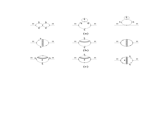
Figure 7: Typical Feynman diagrams for the contribution of quarks and scalar quarks with gluons and gluinos to Higgs–boson self–energies at the two–loop level.

Contrary to the $\Delta\rho$ case the three sets of diagrams do not independently give an ultraviolet finite result for the renormalized $\Phi$ self–energy. In addition it is necessary to make use of DRED. By explicit calculations both in DREG and in DRED, we found a finite result only for the DRED. The same observation has been made also in $\!{}^{{\bf?}}$ for the two–loop calculation of the upper bound for $m_{h}$.

7.2 Calculation of $m_{h}$

The mass matrix at two–loop order is given in terms of the tree–level masses and of the one– and two–loop renormalized $\Phi$ self–energies which can be diagonalized by the angle $\alpha_{\rm eff}$

$${\cal L}_{2}=\left(\begin{array}[]{cc}m_{\Phi_{1}}^{2}-\hat{\Sigma}_{\Phi_{1}}^{1}-\hat{\Sigma}_{\Phi_{1}}^{2}&m_{\Phi_{1}\Phi_{2}}^{2}-\hat{\Sigma}_{\Phi_{1}\Phi_{2}}^{1}-\hat{\Sigma}_{\Phi_{1}\Phi_{2}}^{2}\\ m_{\Phi_{1}\Phi_{2}}^{2}-\hat{\Sigma}_{\Phi_{1}\Phi_{2}}^{1}-\hat{\Sigma}_{\Phi_{1}\Phi_{2}}^{2}&m_{\Phi_{2}}^{2}-\hat{\Sigma}_{\Phi_{2}}^{1}-\hat{\Sigma}_{\Phi_{2}}^{2}\end{array}\right)\stackrel{{\scriptstyle\alpha_{\rm eff}}}{{\longrightarrow}}\left(\begin{array}[]{cc}m_{H}^{2}&0\\ 0&m_{h}^{2}\end{array}\right),$$ (36)

where $m_{H,h}$ denote the heavy and light Higgs masses at two–loop.

Due to the gluino–exchange contribution the analytical result is very complicated, it will be given in $\!{}^{{\bf?}}$. The numerical results are displayed in Fig. 8 for $m_{h}$ at the tree–, the one– and the two–loop level as a function of $m_{\tilde{q}}$ for the same scenario as in Sec. 5 but with $\tan\beta\hskip 2.84526pt=1.6$ and $40$, $m_{\tilde{g}}=500$ GeV and $M_{A}=200$ GeV ($M_{t}^{LR}=0$ GeV.)

Figure 8: The mass of the lightest MSSM Higgs boson $m_{h}$ displayed as a function of $m_{\tilde{q}}$ for two values of $\tan\beta\hskip 2.84526pt$, $m_{\tilde{g}}=500\mbox{ GeV },M_{A}=200\mbox{ GeV }$

The two–loop result lowers the one–loop mass by about $15$ GeV. The decrease is even somewhat larger for small $\tan\beta\hskip 2.84526pt$. This strengthens for the small $\tan\beta\hskip 2.84526pt$ scenario, which is favoured by SU(5) GUT scenarios, the discovery potential of LEP2.

References

References

-
[1]
H.P. Nilles, Phys. Rep.
110, 1 (1984);
H.E. Haber and G.L. Kane, Phys. Rep. 117, 75 (1985);
R. Barbieri, Riv. Nuovo Cim. 11, 1 (1988). - [2] Particle Data Group, Phys. Rev. D54, (1996) 1.
-
[3]
P. Chankowski, A. Dabelstein, W. Hollik, W. Mösle, S. Pokorski and
J. Rosiek , Nucl. Phys. B 417 (1994) 101;
D. Garcia and J. Solà, Mod. Phys. Lett. A 9 (1994) 211. -
[4]
D. Garcia, R. Jimenes and J. Sola, Phys. Lett B 347 (1995) 309;
B347 (1995) 321;
D. Garcia, and J. Sola, Phys. Lett. B 357 (1995) 349;
A. Dabelstein, W. Hollik, W. Mösle, in Perspectives for Electroweak Interactions in Collisions, ed. B. A. Kniehl, World Scientific 1995 (p. 345);
P. Chankowski and S. Pokorski, Nucl. Phys. B 475 (1996) 3;
W. de Boer, A. Dabelstein, W. Hollik, W. Mösle and U. Schwickerath, Z. Phys. C 75 (1997) 627. -
[5]
H.E. Haber, R. Hempfling, Phys. Rev. Lett. 66 (1991) 1815;
Y. Okada, M. Yamaguchi and T. Yanagida, Prog. Theor. Phys. 85 (1991) 1;
J. Ellis, G. Ridolfi and F. Zwirner, Phys. Lett. B 257 (1991) 83. - [6] J.F. Gunion, H.E. Haber, G. Kane, S. Dawson: The Higgs Hunter’s Guide, Addison-Wesley, 1990.
- [7] J. Küblbeck, M. Böhm and A. Denner, Comput. Phys. Commun 60, 165 (1990).
- [8] G. Weiglein, R. Scharf and M. Böhm, Nucl. Phys. B 416 (1994) 606.
-
[9]
G. ’t Hooft, M. Veltman, Nucl. Phys. B 153 (1979) 365;
G. Passarino, M. Veltman, Nucl. Phys. B 160 (1979) 151. -
[10]
W. Siegel, Phys. Lett. B 84 (1979) 193;
D. M. Capper, D.R.T. Jones, P. van Nieuwenhuizen, Nucl. Phys. B 167 (1980) 479. - [11] I. Jack, D. Jones and K. Roberts, Z. Phys. C 63 (1994) 151.
- [12] M. Veltman, Nucl. Phys. B 123 (1977) 89.
- [13] A. Djouadi, P. Gambino, S. Heinemeyer, W. Hollik, C. Jünger and G. Weiglein, Phys. Rev. Lett. 78 (1997) 3626.
- [14] A. Djouadi, P. Gambino, S. Heinemeyer, W. Hollik, C. Jünger and G. Weiglein, hep-ph/9710438.
-
[15]
A. Djouadi and C. Verzegnassi, Phys. Lett. B195 (1987) 265;
A. Djouadi, Nuovo Cim. A 100 (1988) 357. - [16] Heinemeyer et al, in preparation.
- [17] A. Djouadi, P. Gambino, Phys. Rev. D 49 (1994) 3499.
- [18] R. Hempfling, A. Hoang, Phys. Lett. B 331 (1994) 99.
- [19] M. Carena, M. Quiros and C. Wagner, Nucl. Phys. B 461 (1996) 407.
- [20] S. Heinemeyer, W. Hollik and G. Weilein, hep-ph/9803277