Isocurvature Fluctuations of the M-theory Axion in a Hybrid Inflation Model

Abstract

The M-theory, the strong-coupling heterotic string theory, presents various interesting new phenomenologies. The M-theory bulk axion is one of these. The decay constant in this context is estimated as $F_{a}\simeq 10^{16}$ GeV. Direct searches for the M-theory axion seem impossible because of the large decay constant. However, we point out that large isocurvature fluctuations of the M-theory axion are obtained in a hybrid inflation model, which will most likely be detectable in future satellite experiments on anisotropies of cosmic microwave background radiation.

I Introduction

It is widely believed that nonperturbative effects play a central role in describing the real world in superstring theories. Horava and Witten [1] have argued that the strong-coupling heterotic string theory is dual to an M-theory compactified on ${\bf S}^{1}/{\bf Z}_{2}$. The low-energy limit of this M-theory is well described by eleven-dimensional supergravity, where the fundamental energy scale is the eleven-dimensional Planck mass $M_{11}\simeq 6\times 10^{16}$ GeV, rather than the four-dimensional one $M_{4}\simeq 2\times 10^{18}$ GeV [2]. The four-dimensional Planck mass $M_{4}$ is only an effective parameter appearing at low energies.

This M-theory description of strong-coupling heterotic string theory leads to various interesting new phenomenologies. Banks and Dine [3] have pointed out that the bulk moduli fields provide axion candidates in the M-theory compactified further on a Calabi-Yau manifold, and some of the axions survive at low energies, since world-sheet instanton effects are suppressed owing to the large compactification radius in the string tension unit. One of the string axions may acquire its mass dominantly from the QCD anomaly, and it plays the role of the Peccei-Quinn axion [4] in solving the strong $CP$ problem.

The decay constant $F_{a}$ of the M-theory axion is estimated as [3, 5]

$$F_{a}\simeq 10^{16}{\rm GeV}.$$ (1)

This value greatly violates the constraint $10^{10}{\rm GeV}\lesssim F_{a}\lesssim 10^{12}$ GeV, derived in standard cosmology [6]. However, this problem may be solved by late-time entropy production through decays of moduli fields [7, 8] or a thermal inflaton field [9]. Since a very low reheating temperature, such as $T_{R}\simeq 1$ - $10$MeV, is required to solve the above problem, it is hard to imagine a consistent production of the lightest supersymmetric (SUSY) particles, and they cannot be the dark matter [10]. Thus, the M-theory axion seems the most plausible candidate for the dark matter in our universe.

If the M-theory axion is indeed the dark matter, fluctuations of the axion density should consist of mixtures of adiabatic and isocurvature modes in general [11, 12, 13]. In this paper we show that a hybrid inflation model proposed by Linde and Riotto [14] naturally produces isocurvature fluctuations of the axion comparable to the adiabatic fluctuations that are in the accessible range of future satellite experiments on anisotropies of the cosmic microwave background radiation (CMB). The present analysis, therefore, confirms the previous proposal [15].

II Hybrid inflation model

Let us now discuss the hybrid inflation model [14], which contains two kinds of superfields. One of these fields is $S(x,\ \theta)$ and the others are $\psi(x,\ \theta)$ and $\bar{\psi}(x,\ \theta)$. The model is based on $U(1)_{R}$ symmetry under which $S(\theta)\to e^{2i\alpha}S(\theta e^{-i\alpha})$ and $\psi(\theta)\bar{\psi}(\theta)\to\psi(\theta e^{-i\alpha})\bar{\psi}(\theta e^{-i\alpha})$. The superpotential is then given by

$$W=S(-\mu^{2}+\kappa\bar{\psi}\psi),$$ (2)

where $\mu$ is a mass scale and $\kappa$ a coupling constant. The scalar potential obtained from this superpotential, in the global SUSY limit, is

$$V=\left|-\mu^{2}+\kappa\bar{\psi}\psi\right|^{2}+\kappa^{2}\left|S\right|^{2}\left(\left|\psi\right|^{2}+\left|\bar{\psi}\right|^{2}\right)+D{\rm-terms},$$ (3)

where scalar components of the superfields are denoted by the same symbols as the corresponding superfields. The potential minimum,

$$\langle S\rangle=0,\ \langle\psi\rangle\langle\bar{\psi}\rangle=\frac{\mu^{2}}{\kappa},\ \left|\langle\psi\rangle\right|=\left|\langle\bar{\psi}\rangle\right|,$$ (4)

lies in the $D$-flat direction $\left|\psi\right|=|\bar{\psi}|$. By the appropriate gauge and $R$-transformations in this $D$-flat direction, we can bring the complex $S,\ \psi$ and $\bar{\psi}$ fields on the real axis:

$$S\equiv\frac{1}{\sqrt{2}}\sigma,\ \psi=\bar{\psi}\equiv\frac{1}{2}\phi,$$ (5)

where $\sigma$ and $\phi$ are canonically normalized real scalar fields. The potential in the $D$-flat directions then becomes

$$V(\sigma,\ \phi)=\left(-\mu^{2}+\frac{1}{4}\kappa\phi^{2}\right)^{2}+\frac{1}{4}\kappa^{2}\sigma^{2}\phi^{2},$$ (6)

and the absolute potential minimum appears at $\sigma=0,\ \phi=\bar{\phi}=\mu/\sqrt{\kappa}$. However, for $\sigma>\sigma_{c}\equiv\sqrt{2}\mu/\sqrt{\kappa}$, the potential has a minimum at $\phi=0$. The potential given by Eq.(6) for $\phi=0$ is exactly flat in the $\sigma$ direction. The one-loop corrected effective potential (along the inflationary trajectory $\sigma>\sigma_{c}$ with $\phi=0$) is given by [16]

$$V_{\rm one-loop} = \frac{\kappa^{2}}{128\pi^{2}}\left[(\kappa\sigma^{2}-2\mu^{2})^{2}\ln{\frac{\kappa\sigma^{2}-2\mu^{2}}{\Lambda^{2}}}\right.$$ (7)

$$+ \left.(\kappa\sigma^{2}+2\mu^{2})^{2}\ln\frac{\kappa\sigma^{2}+2\mu^{2}}{\Lambda^{2}}-2\kappa^{2}\sigma^{4}\ln{\frac{\kappa\sigma^{2}}{\Lambda^{2}}}\right],$$ (8)

where $\Lambda$ indicates the renormalization scale.

Next, let us consider the supergravity (SUGRA) effects on the scalar potential (ignoring the one-loop corrections calculated above). The $R$-invariant Kähler potential is given by [17]

$$K(S,\psi,\bar{\psi})=\left|S\right|^{2}+\left|\psi\right|^{2}+\left|\bar{\psi}\right|^{2}-\frac{\beta}{4}\left|S\right|^{4}+\cdots,$$ (9)

where the ellipsis denotes higher order terms, which we neglect in the present analysis. Here, we set the gravitational scale $\sim 2.4\times 10^{18}$ GeV equal to unity. Then, the scalar potential becomes [18]

$$V(\sigma,\ \phi) = \exp\left(\frac{\sigma^{2}}{2}-\frac{\beta}{16}\sigma^{4}+\frac{\phi^{2}}{2}\right)\left[\frac{1}{4}\kappa^{2}\phi^{2}\sigma^{2}\left(1+\frac{\phi^{2}}{4}-\frac{\mu^{2}}{\kappa}\right)\right.$$ (11)

$$+\left.\left(1+\frac{\beta-1}{2}\sigma^{2}+\frac{\beta^{2}+\beta+1}{4}\sigma^{4}\right)\left(-\mu^{2}+\frac{\kappa}{4}\phi^{2}\right)^{2}\right].$$

As in the global SUSY case, for $\sigma\gtrsim\sigma_{c}$ the potential has a minimum at $\phi=0$. The scalar potential for $\sigma\gtrsim\sigma_{c}$ and $\phi=0$ becomes

$$V_{\rm SUGRA}=\mu^{4}\left(1+\frac{\beta}{2}\sigma^{2}+\frac{4\beta^{2}+7\beta+2}{16}\sigma^{4}+\cdots\right).$$ (12)

In the first approximation, we assume that the inflaton potential for $\sigma\gtrsim\sigma_{c}$ and $\phi=0$ is given by the simple sum of the one-loop corrections Eq.(7) and the SUGRA potential Eq. (12):

$$V(\sigma) = \mu^{4}\left(1+\frac{\beta}{2}\sigma^{2}+\frac{4\beta^{2}+7\beta+2}{16}\sigma^{4}\right)$$ (13)

$$+ \frac{\kappa^{2}}{128\pi^{2}}\left[(\kappa\sigma^{2}-2\mu^{2})^{2}\ln{\frac{\kappa\sigma^{2}-2\mu^{2}}{\Lambda^{2}}}\right.$$ (14)

$$+ \left.(\kappa\sigma^{2}+2\mu^{2})^{2}\ln\frac{\kappa\sigma^{2}+2\mu^{2}}{\Lambda^{2}}-2\kappa^{2}\sigma^{4}\ln{\frac{\kappa\sigma^{2}}{\Lambda^{2}}}\right].$$ (15)

Hereafter, we study the dynamics of the hybrid inflation with this potential.

We suppose that the inflaton $\sigma$ is chaotically distributed in space at the Planck time and it happens in some region in space that $\sigma$ is approximately the gravitational scale and $\phi$ is very small ($\approx 0$). Then, the inflaton $\sigma$ rolls slowly down the potential, and the region inflates and dominates the universe eventually. During the inflation, the potential assumes an almost constant value. Also the Hubble parameter changes only very slightly and it is given by $H_{I}=V^{1/2}/\sqrt{3}\simeq\mu^{2}/\sqrt{3}$. When $\sigma$ reaches the critical value $\sigma_{c}$, a phase transition occurs and the inflation ends. In order to solve the flatness and horizon problem we need an e-folding number $N$ $\simeq 60$ [6]. In addition, the adiabatic density fluctuations during the inflation should account for the observation by COBE, which leads to [19]

$$\left.\frac{V^{3/2}}{V^{\prime}}\right|_{N=60}\simeq 5.3\times 10^{-4}.$$ (16)

The evolutions for $\sigma$ and $N$ are described by

$$\dot{\sigma} = -\frac{V^{\prime}}{3H},$$ (17)

$$\dot{N} = -H,$$ (18)

which are numerically integrated with $\sigma|_{N=0}=\sigma_{c}$ and Eq. (16) as boundary conditions. Though the inflaton potential is parametrized by three parameters ($\kappa,\ \beta$, and $\mu$), we can reduce the number of the free parameters from three to two by using the constraint Eq. (16). We consider $\mu$ as a function of $\kappa$ and $\beta$, i.e. $\mu=\mu(\kappa,\ \beta)$.

When $\sigma\gtrsim 1$, the slow roll approximation cannot be maintained. Therefore, if the obtained value of $\sigma|_{N=60}\equiv\sigma_{0}$ is larger than the gravitational scale, we should discard those parameter regions. Also, one of the attractions of the hybrid inflation model is that one does not have to invoke extremely small coupling constants. Thus we assume all of the coupling constants $\kappa$ and $\beta$ to have values of ${\cal O}(1)$. Here, we choose $10^{-2}\lesssim\kappa,\ \beta\lesssim 10^{-1}$ as a “reasonable parameter region” (when $\kappa,\ \beta\gtrsim 10^{-1}$, $\sigma_{0}$ exceeds unity, and $N$ cannot be as large as 60). The result is shown in Fig. 1, where we plot the Hubble parameter during the inflation, $H_{I}=\mu^{2}/\sqrt{3}$, as a function of $\kappa$ and $\beta$. One may see easily from Fig. 1 that $H_{I}$ is large ($H_{I}\sim{\cal O}(10^{11-12}{\rm GeV})$) with the reasonable values of the coupling constants $10^{-2}\lesssim\kappa,\ \beta\lesssim 10^{-1}$. When $H_{I}$ has such a large value, the inflation should generate large isocurvature fluctuations of the axion, if it exists. In the above calculations, we have neglected the isocurvature fluctuations. Hence, to be consistent, we must take account of the effects of the isocurvature fluctuations when we normalize the inflaton potential by COBE; i.e., we must modify Eq. (16). We will estimate $H_{I}$ taking account of the isocurvature effects later.

III Isocurvature fluctuations

We now evaluate the contribution of the isocurvature fluctuations assuming the existence of the M-theory axion. Kawasaki, Sugiyama and Yanagida [13] defined $\alpha$ as the ratio of the initial entropy perturbation to the adiabatic one when the universe is radiation dominant, and found it to assume the form 

$$\alpha_{\rm KSY}=\frac{9(V^{\prime})^{2}}{4H_{I}^{4}F_{a}^{2}\theta^{2}}.$$ (19)

Here, $F_{a}\theta$ is the initial value of the axion field. In this paper, we redefine $\alpha$ as the ratio of the present (the universe is matter dominant) matter power spectra. Therefore, in our notation, $\alpha=1$ implies that the adiabatic and the isocurvature matter power spectra have the same value in the long wavelength limit. The old version $\alpha_{\rm KSY}$ in Eq. (19) is related to our new version $\alpha$ as

$$\alpha=\left(\frac{2}{15}\right)^{2}\left(\frac{10}{9}\right)^{2}\alpha_{\rm KSY}=\left(\frac{4}{27}\right)^{2}\alpha_{\rm KSY}=\frac{4(V^{\prime})^{2}}{81H_{I}^{4}F_{a}^{2}\theta^{2}}.$$ (20)

The isocurvature fluctuations give a contribution to the CMB anisotropies which are about six times larger than the adiabatic ones in the long wavelength limit. At the COBE scales, this factor somehow decreases, and the precise value depends on $\Omega_{0}$ and $h$, and is a monotonically increasing function of these parameters. Here, $\Omega_{0}$ is the ratio of the present energy density to the critical density, and $h$ is the present Hubble parameter normalized by $100$ km s^-1 Mpc^-1. If we take $\Omega_{0}\simeq 1$ and $h\simeq 0.6$, the factor is approximately $\sqrt{30}$. Therefore, when we take account of the isocurvature fluctuations, the correct COBE normalization becomes

$$\left.\frac{V^{3/2}}{V^{\prime}}\right|_{N=60}\simeq\frac{5.3\times 10^{-4}}{\sqrt{1+30\alpha}},$$ (21)

rather than Eq. (16). Here, we have ignored the tensor perturbations since they are negligibly small in our model. Note that the spectral index is almost unity in our model.

From Eqs. (19), (20), and (21), one may see that

$$\frac{1+30\alpha}{\alpha}\simeq 21\times\left(\frac{H_{I}}{10^{12}{\rm GeV}}\right)^{-2}\left(\frac{F_{a}\theta}{10^{16}{\rm GeV}}\right)^{2}.$$ (22)

For the M-theory axion, the decay constant $F_{a}$ is estimated as $F_{a}\simeq\ 10^{16}$ GeV [3, 5]. This value is much larger than the constraint on $F_{a}$, $F_{a}\lesssim 10^{12}$ GeV, which comes from the requirement that the axion should not overclose the universe. However, as shown in Ref. [7] this constraint is greatly relaxed if late-time entropy production occurs. In this case, the unclosure condition for the present universe leads to an upper bound on $F_{a}\theta$ :

$$F_{a}\theta\lesssim 4.4\times 10^{15}{\rm GeV}.$$ (23)

Here the reheating temperature after late-time entropy production is taken as $T_{R}=1$ MeV. Thus, a decay constant $F_{a}\simeq\ 10^{16}$ GeV of the M-theory axion is allowed if we take $\theta\lesssim 0.3$, which is not an unnaturally small value. If one takes $F_{a}\theta\simeq 10^{12}$ GeV as in the standard invisible axion model, the isocurvature fluctuations become too large. Thus the large value of $F_{a}$ for the M-theory axion is a rather crucial point in our mixed fluctuation model.

We are at the point of evaluating $\alpha$, which depends on two parameters $F_{a}\theta$ and $H_{I}$, as seen from Eq. (22). We take $H_{I}\simeq 10^{11-12}$ GeV, which has been obtained for the case of $\alpha=0$. We have, however, found that similar values of the Hubble constant $H_{I}$ are obtained even for $\alpha\neq 0$, as long as $\left|\alpha\right|\lesssim 1$. In Fig. 2 we plot $H_{I}$ for $\alpha=0.01$ as an example. From Eq. (22) we derive $\alpha\gtrsim 0.003$ for $F_{a}\theta\lesssim 4\times 10^{15}$ GeV and $H_{I}\simeq 10^{11-12}$ GeV.

IV Discussion

The mixture of isocurvature and adiabatic fluctuations is astrophysically interesting. Since isocurvature fluctuations yield anisotropies of the CMB that are six times larger than those caused by adiabatic fluctuations, mixed fluctuations reduce the amplitude of the power spectrum if the amplitude is normalized by COBE. It is well known that the standard cold dark matter scenario ($\Omega_{0}=1,h=0.5$) with COBE-normalized pure adiabatic fluctuations predicts density fluctuations that are too large on scales of galaxies and clusters. This problem is avoided if the isocurvature fluctuations are mixed with adiabatic ones, as is pointed in Ref. [13]. Furthermore, it can be shown that for the general flat universe ($\lambda_{0}+\Omega_{0}=1$, with $\lambda_{0}$ the cosmological constant), the shape and amplitude of the power spectrum are in good agreement with observations if $\alpha\sim 0.05$ [21].

The CMB anisotropies induced by the isocurvature fluctuations can be distinguished from those produced by pure adiabatic fluctuations [13], because the shapes of the angular power spectrum of CMB anisotropies are quite different from each other on small angular scales. The most significant effect of the mixture of the isocurvature fluctuation is that the acoustic peak in the angular power spectrum decreases. In Fig. 3 we show the angular power spectrum for $\alpha=0.05$, $\Omega_{0}=0.4$ and $h=0.7$ as an example. It is seen that the height of the acoustic peak ($\ell\sim 200$) in the case of mixed fluctuations is greatly reduced compared with the pure adiabatic case.

Since the axion decay constant $F_{a}$ is much higher than $10^{12}$ GeV, a direct search for the M-theory axion is implausible. Therefore, observations of CMB anisotropies by future satellite experiments (MAP [22], PLANCK [23]) are very crucial to test the M-theory axion hypothesis.

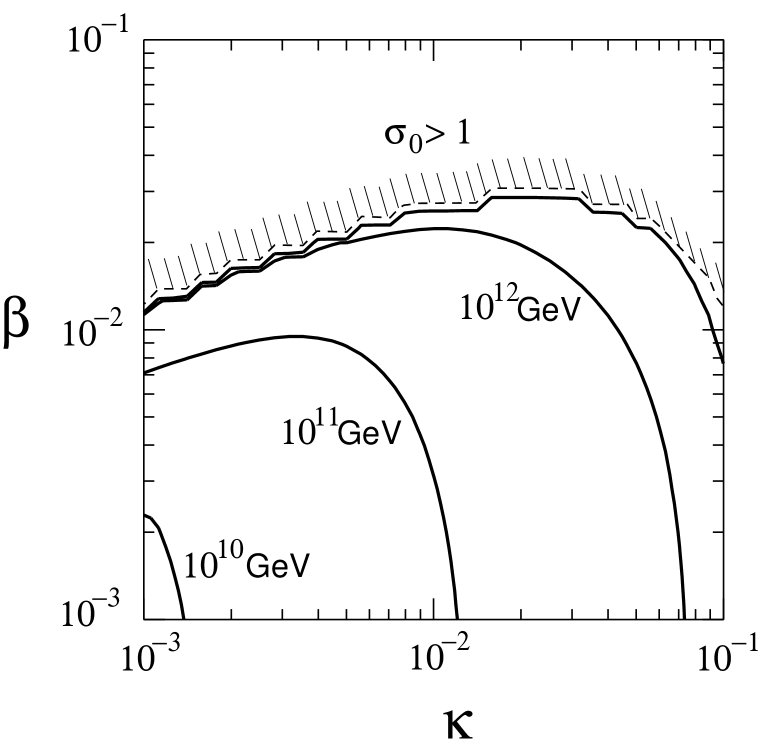
FIG. 1.: The Hubble parameter $H_{I}$ during the inflation, normalized by the COBE, ignoring tensor perturbations and isocurvature fluctuations. In the region above the dashed line, $\sigma_{0}$ exceeds the gravitational scale, $\sigma_{0}>1$, and it is excluded.

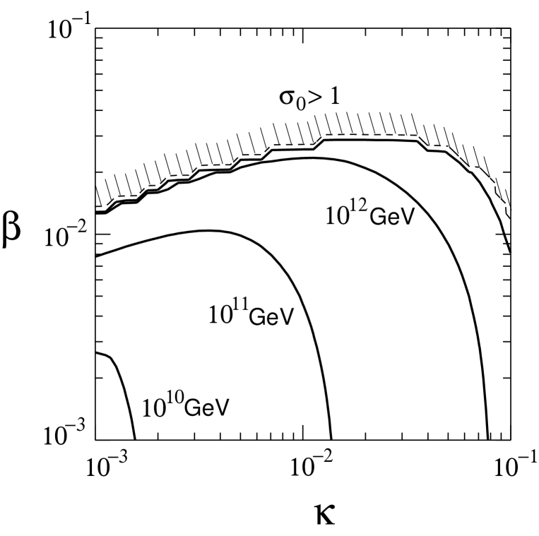
FIG. 2.: The Hubble parameter $H_{I}$ during the inflation, normalized by the COBE for the $\alpha=0.01$ case, ignoring tensor perturbations. In the region above the dashed line, $\sigma_{0}$ exceeds the gravitational scale, $\sigma_{0}>1$, and it is excluded.

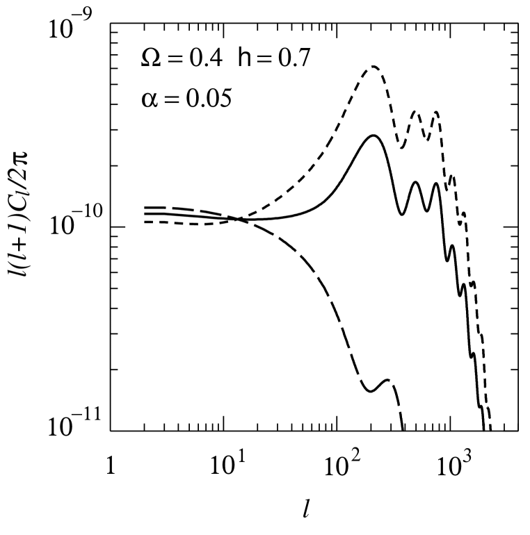
FIG. 3.: The CMB angular power spectra normalized by the COBE. Here, we have chosen $\Omega_{0}=0.4,\ h=0.7,\ \lambda_{0}=0.6$, and $\Omega_{B}h^{2}=0.015$. The short dashed line corresponds to the pure adiabatic case ($\alpha=0$), the long dashed line to the pure isocurvature case ($\alpha=\infty$), and the solid line to the case $\alpha=0.05$.

REFERENCES

- [1] P. Horava and E. Witten, Nucl. Phys. B460, 506 (1996); Phys. Rev. D54, 7561 (1996).
- [2] E. Witten, Nucl. Phys. B471, 135 (1996).
- [3] T. Banks and M. Dine, Nucl. Phys. B479, 173 (1996); Nucl. Phys. B505, 445 (1997).
- [4] R. D. Peccei and H. R. Quinn, Phys. Rev. Lett. 38, 1440 (1977).
-
[5]
K. Choi, Phys. Rev. D56, 6588 (1997);
K. Choi and J. E. Kim, Phys. Lett. B154, 393 (1985). - [6] E. W. Kolb and M. S. Turner, The Early Universe (Addison-Wesley, 1990).
- [7] M. Kawasaki, T. Moroi and T. Yanagida, Phys. Lett. B383, 313 (1996).
- [8] T. Banks and M. Dine, Nucl. Phys. B505, 445 (1997).
- [9] D. H. Lyth and E. D. Stewart, Phys. Rev. D53, 1784 (1996).
- [10] M. Kawasaki, T. Moroi and T. Yanagida, Phys. Lett. B370, 52 (1996).
-
[11]
M.S. Turner and F. Wilczek,
Phys. Rev. Lett. 66, 5 (1991);
A.D. Linde, Phys. Lett. B259, 38 (1991). - [12] D.H. Lyth, Phys. Lett. 236, 408 (1990); Phys. Rev. D45, 3394 (1992).
- [13] M. Kawasaki, N. Sugiyama and T. Yanagida, Phys. Rev. D54, 2442 (1996).
- [14] A. Linde and A. Riotto, Phys. Rev. D56, 1841 (1997).
- [15] M. Kawasaki and T. Yanagida, Prog. Theor. Phys. 97, 809 (1997).
- [16] G. Dvali, Q. Shafi and R. Schaefer, Phys. Rev. Lett. 73, 1886 (1994).
- [17] C. Panagiotakopoulos, Phys. Lett. B402, 257(1997).
- [18] For a review, H. P. Nilles, Phys. Rep. 110, 1 (1984).
- [19] C. L. Bennett et al., Astrophys. J. 464, L1 (1996).
- [20] H. Kodama and M. Sasaki, Int. J. Mod. Phys. A1, 265 (1986); A2, 491 (1987).
- [21] T. Kanazawa, M. Kawasaki, N. Sugiyama and T. Yanagida, in preparation.
- [22] http://map.gsfc.nasa.gov/.
- [23] http://astro.estec.esa.nl/SA-general/Projects/Planck/.