Extraction of the $D^{*}D\pi$ coupling from $D^{*}$ decays

Abstract

The decays $D^{*}\to D\pi$ and $D^{*}\to D\gamma$ are well described by heavy meson chiral perturbation theory. With the recent measurement of ${\cal B}(D^{*+}\to D^{+}\gamma$), the $D^{*0}$, $D^{*+}$, and $D_{s}^{*}$ branching fractions can be used to extract the $D^{*}D\pi$ and $D^{*}D\gamma$ couplings $g$ and $\beta$. The $D^{*}\to D\gamma$ decays receive important corrections at order $\sqrt{m_{q}}$ and, from the heavy quark magnetic moment, at order $1/m_{c}$. Here all the decay rates are computed to one-loop, to first order in $m_{q}$ and $1/m_{c}$, including the effect of heavy meson mass splittings, and the counterterms at order $m_{q}$. A fit to the experimental data gives two possible solutions, $g=0.27\,^{+.04}_{-.02}\,{}^{+.05}_{-.02}$, $\beta=0.85^{+.2}_{-.1}\,{}^{+.3}_{-.1}\,{\rm GeV^{-1}}$ or $g=0.76\,^{+.03}_{-.03}\,{}^{+.2}_{-.1}$, $\beta=4.90^{+.3}_{-.3}\,{}^{+5.0}_{-.7}\,{\rm GeV^{-1}}$. The first errors are experimental, while the second are estimates of the uncertainty induced by the counterterms. (The experimental limit $\Gamma_{D^{*+}}<0.13\,{\rm MeV}$ excludes the $g=0.76$ solution.) Predictions for the $D^{*}$ and $B^{*}$ widths are given.

I Introduction

Combining chiral perturbation theory with heavy quark effective theory (HQET) gives a good description of the low energy strong interactions between the pseudo-goldstone bosons and mesons containing a single heavy quark. Due to heavy quark symmetry (HQS)[1] there is one coupling, $g$, for $D^{*}D\pi$, $D^{*}D^{*}\pi$, $B^{*}B\pi$, and $B^{*}B^{*}\pi$, and one coupling, $\beta$, for $D^{*}D\gamma$, $D^{*}D^{*}\gamma$, $B^{*}B\gamma$, and $B^{*}B^{*}\gamma$ at leading order. The value of the coupling $g$ is important, since it appears in the expressions for many measurable quantities at low energy. These include the rate $B\to D^{(*)}\pi\ell\bar{\nu}_{\ell}$ [2], form factors for weak transitions between heavy and light pseudo-scalars [3, 4, 5], decay constants for the heavy mesons [6, 7], weak transitions to vector mesons [8], form factors for $B\to D^{(*)}\ell\bar{\nu}_{\ell}$ [9], and heavy meson mass splittings [10] (for a review see [11]). However, the value of $g$ has remained somewhat elusive, with numbers in the literature from $\sim 0.2$ to $1.0$. Recently, a CLEO measurement [12] of $D^{*+}\to D^{+}\gamma$ has brought the experimental uncertainties to a level where a model independent extraction of $g$ is possible from $D^{*}$ decays.

As a consequence of HQS the mass splitting between $D^{*}$ and $D$ mesons is small (of order $\Lambda_{\rm QCD}^{2}/m_{c}$), leaving only a small amount of phase space for $D^{*}$ decays. In the dominant modes, $D^{*}\to D\pi$, and $D^{*}\to D\gamma$, the outgoing pion and photon are soft making the chiral expansion a valid framework. The branching ratios for $D^{*+}$ decay are $D^{0}\,\pi^{+}$ (67.6%), $D^{+}\,\pi^{0}$ (30.7%) and $D^{+}\,\gamma$ (1.7%) [12]. A $D^{*0}$ can only decay into $D^{0}\,\pi^{0}$ (61.9%) and $D^{0}\gamma$ (38.1%) [13] since there is not enough phase space for $D^{+}\,\pi^{-}$. The $D^{*}_{s}$ decays predominantly to $D_{s}\,\gamma$ (94.2%) with a small amount going into the isospin violating mode $D_{s}\,\pi^{0}$ (5.8%) [13]. Since a measurement of the widths of the $D^{*}$ mesons has not yet been made, it is only possible to compare the ratios of branching fractions with theoretical predictions. The ratio $R_{\pi}^{+}={\cal B}(D^{*+}\to D^{0}\pi^{+})/{\cal B}(D^{*+}\to D^{+}\pi^{0})$ is fixed by isospin to be $R_{\pi}^{+}=2|\vec{k}_{\pi^{+}}|^{3}/|\vec{k}_{\pi^{0}}|^{3}=2.199\pm 0.064$ [12] (where $\vec{k}_{\pi^{+,0}}$ are three momenta for the outgoing pions in the $D^{*}$ rest frame). This value is often used in experimental extractions of the branching ratios to reduce systematic errors.

It is interesting to note that the quark model predictions[14] for $D^{*0}$ and $D^{*+}$ decays agree qualitatively with the data. One can understand, for instance, why the branching ratio ${\cal B}(D^{*+}\to D^{+}\gamma)$ is small compared to ${\cal B}(D^{*0}\to D^{0}\gamma)$. In the quark model the photon couples to the meson with a strength proportional to the sum of the magnetic moments of the two quarks, $\mu_{2}=2/(3\,m_{c})-1/(3\,m_{d})$ for $D^{*+}\to D^{+}\gamma$ and $\mu_{1}=2/(3\,m_{c})+2/(3\,m_{u})$ for $D^{*0}\to D^{0}\gamma$. The rate for the former is then suppressed by a factor

$$\left|\frac{\mu_{2}}{\mu_{1}}\right|^{2}=(m_{u}/m_{d})^{2}{(m_{d}/m_{c}-1/2)^{2}\over(m_{u}/m_{c}+1)^{2}}\simeq 0.04\>,$$ (1)

where we have used mass ratios appropriate for constituent quarks, $m_{u}/m_{d}\simeq 1$, $m_{d}/m_{c}\simeq m_{u}/m_{c}\simeq 1/4$. This suppression results from the opposite signs in $\mu_{1}$ and $\mu_{2}$, which in turn follow from the (quark) charge assignments and spin wavefunctions for the heavy mesons.

In the quark model $g=1$ and $\beta\simeq 3\,{\rm GeV^{-1}}$, while for the chiral quark model $g=0.75$ [15]. Relativistic quark models tend to give smaller values, $g\sim 0.4$ [16], as do QCD sum rules, $g\sim 0.2-0.4$ [17].

Our purpose here is to use heavy meson chiral perturbation theory at one-loop to extract the couplings $g$ and $\beta$ from $D^{*}$ decays. In other words, we wish to examine how sensitive a model independent extraction of $g$ and $\beta$ is to higher order corrections. For $D^{*}\to D\gamma$, analyses beyond leading order have included the heavy quark’s magnetic moment which arises at $1/m_{c}$ [18, 19], and the leading non-analytic effects from chiral loops proportional to $\sqrt{m_{q}}$ [18]. $\sqrt{m_{q}}$ terms proportional to both $m_{K}$ and $m_{\pi}$ were found to be important. These effects do not introduce any new unknown quantities into the calculation of the decay rates. For $D^{*}\to D\gamma$ and the isospin conserving $D^{*}\to D\pi$ decays the effect of chiral logarithms, $m_{q}\ln{(\mu/m_{q})}$, have also been considered [20]. These are formally enhanced over other $m_{q}$ corrections in the chiral limit, $m_{q}\to 0$, however, the choice of the scale $\mu$ leads to some ambiguity in their contribution. (This scale dependence is cancelled by unknown couplings which arise at order $m_{q}$ in the chiral Lagrangian.) The isospin violating decay $D_{s}^{*}\to D_{s}\pi^{0}$ has only been considered at leading order, where it occurs through $\eta-\pi^{0}$ mixing[21].

In this paper the investigation of all $D^{*}$ decays is extended to one-loop, including symmetry breaking corrections to order $m_{q}$ and $1/m_{c}$. Further $1/m_{c}$ and $m_{q}$ contributions considered here include the effect of nonzero $D^{*}$–$D$ and $D_{s}$–$D^{0}$ mass splittings, and the exact kinematics corresponding to nonzero outgoing pion or photon energy in the loop diagrams. (Their inclusion is motivated numerically since $m_{\pi^{0}}\sim m_{D^{*}}-m_{D}\sim m_{D_{s}}-m_{D}$, and the decay $D^{*}\to D\pi^{0}$ only occurs if $m_{D^{*}}-m_{D}>m_{\pi^{0}}$.) To simplify the organization of the calculation these splittings will be included as residual mass terms in our heavy meson propagators. This gives new non-analytic contributions to the $D^{*}\to D\pi^{0}$ and $D^{*}\to D\gamma$ decay rates. (To treat the mass splittings as perturbations one can simply expand these non-analytic functions.) At order $m_{q}$ there are also analytic contributions due to new unknown couplings which are discussed. These new couplings can, in principle, be fixed using other observables. We estimate the effect these unknown couplings have on the extraction of $g$ and $\beta$.

The calculation of the decay rates to order $m_{q}$ and $1/m_{c}$ is taken up in section II. In section III we compare the theoretical partial rates with the data to extract the $D^{*}D\pi$ and $D^{*}D\gamma$ couplings and discuss the uncertainty involved. Predictions for the widths of the $D^{*}$ and $B^{*}$ mesons are also given. Conclusions can be found in section IV.

II Decay rates for $D^{*0}$, $D^{*+}$, and $D_{s}^{*}$

In this section we construct the effective chiral Lagrangian that describes the decays $D^{*}\to D\pi$ and $D^{*}\to D\gamma$ to first order in the symmetry breaking parameters $m_{q}$ and $1/m_{c}$. The eight pseudo-goldstone bosons $\pi^{i}$ that arise from the breaking $SU(3)_{L}\times SU(3)_{R}\rightarrow SU(3)_{V}$ are identified with the pseudoscalar mesons ($\pi^{0}$,$\pi^{+}$,$\pi^{-}$,$K^{0}$,$\bar{K}^{0}$,$K^{+}$,$K^{-}$,$\eta$). These can be encoded in the exponential representation $\Sigma=\xi^{2}=\exp(2i\pi^{i}\lambda^{i}/f)$, where $\lambda^{i}$ are $3\times 3$ matrices such that

$${\normalsize\pi^{i}\lambda^{i}=\left(\begin{array}[]{ccc}\pi^{0}/\sqrt{2}+\eta/\sqrt{6}&\pi^{+}&K^{+}\\ \pi^{-}&-\pi^{0}/\sqrt{2}+\eta/\sqrt{6}&K^{0}\\ K^{-}&\bar{K}^{0}&-2\eta/\sqrt{6}\end{array}\right)\,,}$$ (5)

and $f\sim f_{\pi}=130\,{\rm MeV}$. For the triplets of heavy mesons ($D^{0}$, $D^{+}$, $D_{s}$) and ($D^{*0}$, $D^{*+}$, $D_{s}^{*}$) we use the velocity dependent fields $P_{a}(v)$ and $P_{a}^{*\mu}(v)$ (a=1,2,3) of HQET. These are included in a $4\times 4$ matrix which transforms simply under heavy quark symmetry

$$H_{a}=\frac{1+v\!\!\!/}{2}\,\Big{[}P_{a}^{*\mu}\gamma_{\mu}-P_{a}\,\gamma_{5}\Big{]}\,,$$ (6)

and satisfies $v\!\!\!/H_{a}=H_{a}=-H_{a}v\!\!\!/$. Including the quark mass term $m_{q}={\rm diag}(m_{u},m_{d},m_{s})$ the lowest order Lagrangian is then [3]

$${\cal L}_{0} = \frac{f^{2}}{8}{\rm Tr}\,\partial^{\mu}\Sigma\,\partial_{\mu}\Sigma^{\dagger}+{f^{2}B_{0}\over 4}{\rm Tr}(m_{q}\Sigma+m_{q}\Sigma^{\dagger})-{\rm Tr}\,\bar{H}_{a}iv\cdot D_{ba}H_{b}+g\,{\rm Tr}\,\bar{H}_{a}H_{b}\gamma_{\mu}\gamma_{5}A^{\mu}_{ba}\,,$$ (7)

where the derivative $D^{\mu}_{ab}=\delta_{ab}\,\partial^{\mu}-V_{ab}^{\mu}$, and $\bar{H}_{a}=\gamma^{0}H_{a}^{\dagger}\gamma^{0}$. The vector and axial vector currents, $V_{ab}^{\mu}=\frac{1}{2}(\xi^{\dagger}\partial^{\mu}\xi+\xi\partial^{\mu}\xi^{\dagger})$ and $A_{ab}^{\mu}=\frac{i}{2}(\xi^{\dagger}\partial^{\mu}\xi-\xi\partial^{\mu}\xi^{\dagger})$, contain an even and odd number of pion fields respectively. The Lagrangian in Eq. (7) is invariant under heavy quark flavor and spin symmetry. It is also invariant under chiral $SU(3)_{L}\times SU(3)_{R}$ transformations, where $\Sigma\to L\Sigma R^{\dagger}$, $\xi\to L\xi U^{\dagger}=U\xi R^{\dagger}$, $H\to HU^{\dagger}$, if we take the quark mass (which breaks the chiral symmetry) to transform as $m_{q}\to Lm_{q}R^{\dagger}$.

The last term in Eq. (7) couples $P^{*}P\pi$ and $P^{*}P^{*}\pi$ with strength $g$ and determines the decay rate $D^{*}\rightarrow D\pi$ at lowest order. Going beyond leading order involves including loops with the pseudo-goldstone bosons, as well as higher order terms in the Lagrangian with more powers of $m_{q}$, $1/m_{c}$, and derivatives. At order $m_{q}\sim 1/m_{c}$ the following mass correction terms appear

$${\cal L}_{m}=\frac{\lambda_{2}}{4\,m_{Q}}{\rm Tr}\,\bar{H}_{a}\sigma^{\mu\nu}H_{a}\sigma_{\mu\nu}+2\lambda_{1}{\rm Tr}\,\bar{H}_{a}H_{b}m^{\xi}_{ba}+2\lambda_{1}^{\prime}{\rm Tr}\,\bar{H}_{a}H_{a}m^{\xi}_{bb},$$ (8)

where $m^{\xi}=\frac{1}{2}(\xi m_{q}\xi^{\dagger}+\xi^{\dagger}m_{q}\xi)$. The $\lambda_{1}^{\prime}$ term can be absorbed into the definition of $m_{H}$ by a phase redefinition of $H$. The $\lambda_{2}$ term is responsible for the $D^{*}$-$D$ mass splitting at this order, $\Delta=m_{D^{*}}-m_{D}=-2\lambda_{2}/m_{c}$. The term involving $\lambda_{1}$ splits the mass of the triplets of $D$ and $D^{*}$ states. Ignoring isospin violation this splitting is characterized by $\delta=m_{D_{s}^{*}}-m_{D^{*}}=m_{D_{s}}-m_{D}=2\lambda_{1}(m_{s}-\hat{m})$ where $\hat{m}=m_{u}=m_{d}$. For the purpose of our power counting $\delta\sim m_{q}\sim 1/m_{c}\sim\Delta$. The effect of these mass splitting terms can be taken into account by including a residual mass term in each heavy meson propagator. Since we are interested in decay rates we choose the phase redefinition for our heavy fields to scale out the decaying particle’s mass. For $D^{*0}$ and $D^{*+}$ decays the denominator of our propagators are: $2v\cdot k$ for $D^{*0}$ and $D^{*+}$, $2(v\cdot k-\delta)$ for $D_{s}^{*}$, $2(v\cdot k+\Delta)$ for $D^{0}$ and $D^{+}$, and $2(v\cdot k+\Delta-\delta)$ for $D_{s}$. For the $D_{s}^{*}$ decays the denominators are the above factors plus $2\delta$. (If we scaled out a different mass then the calculation in the rest frame of the initial particle would involve a residual ‘momentum’ for the initial particle, but would yield the same results.) This results in additional non-analytic contributions from one-loop diagrams which are functions of the quantities $\Delta/m_{\pi_{i}}$ and $\delta/m_{\pi_{i}}$. Formally, $m_{\pi_{i}}^{2}\sim m_{q}\sim\Delta\sim\delta$ and one can expand these contributions to get back the result of treating the terms in Eq. (8) as perturbative mass insertions.

Another type of $1/m_{c}$ corrections are those whose coefficients are fixed by velocity reparameterization invariance [22, 7]

$$\delta{\cal L}_{v} = -\frac{1}{2m_{Q}}{\rm Tr}\,\bar{H}_{a}(iD)^{2}_{ba}H_{b}+\frac{g}{m_{Q}}{\rm Tr}\bar{H}_{c}(i\overleftarrow{D}^{\mu}_{ac}v\cdot A_{ba}-iv\cdot A_{ac}\overrightarrow{D}^{\mu}_{ba})H_{b}\gamma_{\mu}\gamma_{5}\,.$$ (9)

The first term here is the HQET kinetic operator, $O_{\rm kin}=\frac{1}{2m_{Q}}\bar{h}_{v}\,(iD)^{2}\,h_{v}$, written in terms of the interpolating fields $P_{a}$ and $P^{*\mu}_{a}$. In conjunction with the HQET chromomagnetic operator, $O_{\rm mag}=\frac{1}{2m_{Q}}\bar{h}_{v}\,\frac{g_{s}}{2}\,\sigma_{\alpha\beta}G^{\alpha\beta}\,h_{v}$, these contributions to the Lagrangian modify the dynamics of the heavy meson states. They give $1/m_{c}$ corrections in the form of time ordered products with the leading order current [23], which induce spin and flavor symmetry violating corrections to the form of the $D^{*}D\pi$ coupling. We account for these corrections by introducing the couplings $g_{1}$ and $g_{2}$ in Eq. (13) below. The last term in Eq. (9) contributes at higher order in our power counting since it is suppressed by both a derivative and a power of $1/m_{c}$.

Further terms that correct the Lagrangian in Eq. (7) at order $m_{q}\sim 1/m_{c}$ include [7]

$$\delta{\cal L}_{g} = \frac{g\kappa_{1}\,B_{0}}{\Lambda_{\chi}^{2}}{\rm Tr}\,\bar{H}_{a}H_{b}\gamma_{\mu}\gamma_{5}A^{\mu}_{bc}m^{\xi}_{ca}+\frac{g\kappa_{1}^{\prime}\,B_{0}}{\Lambda_{\chi}^{2}}{\rm Tr}\,\bar{H}_{a}H_{b}\gamma_{\mu}\gamma_{5}m^{\xi}_{bc}A^{\mu}_{ca}$$ (10)

$$+ \frac{g\kappa_{3}\,B_{0}}{\Lambda_{\chi}^{2}}{\rm Tr}\,\bar{H}_{a}H_{b}\gamma_{\mu}\gamma_{5}A^{\mu}_{ba}m^{\xi}_{cc}+\frac{g\kappa_{5}\,B_{0}}{\Lambda_{\chi}^{2}}{\rm Tr}\,\bar{H}_{a}H_{a}\gamma_{\mu}\gamma_{5}A^{\mu}_{bc}m^{\xi}_{cb}$$ (11)

$$+ \frac{\delta_{2}}{\Lambda_{\chi}}{\rm Tr}\,\bar{H}_{a}H_{b}\gamma_{\mu}\gamma_{5}iv\cdot D_{bc}A_{ca}^{\mu}+\frac{\delta_{3}}{\Lambda_{\chi}}{\rm Tr}\,\bar{H}_{a}H_{b}\gamma_{\mu}\gamma_{5}iD^{\mu}_{bc}v\cdot A_{ca}$$ (12)

$$+ \frac{g_{1}}{m_{Q}}{\rm Tr}\,\bar{H}_{a}H_{b}\gamma_{\mu}\gamma_{5}A^{\mu}_{ba}+\frac{g_{2}}{m_{Q}}{\rm Tr}\,\bar{H}_{a}\gamma_{\mu}\gamma_{5}H_{b}A^{\mu}_{ba}+\ldots\,,$$ (13)

where $D^{\alpha}_{bc}A^{\beta}_{ca}=\partial^{\alpha}A^{\beta}_{ba}+[V^{\alpha},A^{\beta}]_{ba}$ and $\Lambda_{\chi}=4\pi f$. The ellipses here denote terms linear in $m^{\xi}_{-}=\frac{1}{2}(\xi m_{q}\xi^{\dagger}-\xi^{\dagger}m_{q}\xi)$ which contribute to processes with more than one pion, as well as terms with $(iv\cdot D)$ acting on an $H$. For processes with at most one pion and $H$ on-shell the latter terms can be eliminated at this order, regardless of their chiral indices, by using the equations of motion for $H$. The $\kappa_{i}$ coefficients contain infinite and scale dependent pieces which cancel the corresponding contributions from the one-loop $D^{*}\to D\pi$ diagrams. For the $\kappa_{1}$ and $\kappa_{1}^{\prime}$ terms only the combination $\tilde{\kappa}_{1}=\kappa_{1}+\kappa_{1}^{\prime}$ will enter in an isospin conserving manner here. (The combination $\kappa_{1}-\kappa_{1}^{\prime}$ will contribute an isospin violating correction to $R^{+}_{\pi}$.) At a given scale $\mu$, the finite part of $\kappa_{3}$ can be absorbed into the definition of $g$. The decays $D^{*}\to D\pi$ have analytic contributions from $\tilde{\kappa}_{1}$ and $\kappa_{5}$ at order $m_{q}$.

For $m_{Q}=m_{c}$ the term in Eq. (13) involving $g_{1}$ can be absorbed into $g$ (this term only enters into a comparison with $B^{*}$ decays). The term $g_{2}$ breaks the equality of the $D^{*}D\pi$ and $D^{*}D^{*}\pi$ couplings. Since we only need the coupling $D^{*}D^{*}\pi$ in loops we can also absorb $g_{2}$ into the definition of $g$. Thus, our $g$ is defined as the $D^{*}D\pi$ coupling with $1/m_{Q}$ corrections arising in relating it to the couplings for $D^{*}D^{*}\pi$ and $B^{(*)}B^{*}\pi$.

The terms in Eq. (13) involving $\delta_{2}$ and $\delta_{3}$ contribute to $D^{*}\to D\pi^{0}$, entering in a fixed linear combination with the tree level coupling $g$ of the form $g-(\delta_{2}+\delta_{3})v\cdot k/\Lambda_{\chi}$. These are $\sim 10\%$ corrections for the decays $D^{*}\rightarrow D\pi$. The energy of the outgoing pion is roughly the same for all three decays, $v\cdot k\sim.144\,{\rm GeV}$. Therefore, it is impossible to disentangle the contribution of $\delta_{1,2}$ from that of $g$ for these decays, and the extraction of $g$ presented here will implicitly include their contribution. For other processes involving pions with different $v\cdot k$ these counterterms can give a different contribution. This should be kept in mind when this value of $g$ is used in a different context.

Techniques for one-loop calculations in heavy hadron chiral perturbation theory are well known and will not be discussed here. Dimensional regularization is used and the renormalized counterterms are defined by subtracting the pole terms $1/\epsilon-\gamma+\log{(4\pi)}$. The decays $D^{*0}\to D^{0}\pi^{0}$ and $D^{*+}\to D^{+}\pi^{0}$, and $D_{s}^{*}\to D_{s}\pi^{0}$ have decay rates $\Gamma^{1}_{\pi}$, $\Gamma^{2}_{\pi}$, and $\Gamma^{3}_{\pi}$ given by

$$\Gamma^{a}_{\pi} = {g^{2}\over 12\,\pi\,f^{2}}\left|{Z_{\rm wf}^{a}\over Z_{\pi}^{a}}\right|^{2}\>|{\vec{k}}^{\,a}_{\pi}|^{3}\,.$$ (14)

Here ${\vec{k}}^{\,a}_{\pi}$ is the three momentum of the outgoing pion, $Z_{\pi}^{a}$ contains the vertex corrections, and $Z_{\rm wf}^{a}=\sqrt{Z_{D^{*}}^{a}Z_{D}^{a}}$ contains the wavefunction renormalization for the $D^{*}$ and $D$. When the ratio of $\Gamma^{a}_{\pi}$ to the $D^{*}\to D\gamma$ rate is taken $Z_{\rm wf}^{a}$ will cancel out. However, $Z_{\rm wf}^{a}$ does contribute to our predictions for the $D^{*}$ widths, where the ratio $Z_{\rm wf}^{a}/Z_{\pi}^{a}$ will be kept to order $g^{2}$.

FIG. 1.: $D$ and $D^{*}$ wavefunction renormalization graphs. The dashed line represents a pseudo-goldstone boson.

The graphs in Fig. 1 give

$$Z^{a}_{D} = 1+{g^{2}\over(4\pi f)^{2}}(\lambda^{i}_{ab}\lambda^{i\dagger}_{ba})\bigg{\{}[3m_{i}^{2}-6(\Delta+d_{0})^{2}]\log{(\frac{\mu^{2}}{m_{i}^{2}})}+\,3\,G_{1}(m_{i},\Delta+d_{0})\bigg{\}}\,,$$ (15)

$$Z^{a}_{D^{*}} = 1+{g^{2}\over(4\pi f)^{2}}(\lambda^{i}_{ab}\lambda^{i\dagger}_{ba})\bigg{\{}[3m_{i}^{2}-4d_{0}^{2}-2(d_{0}-\Delta)^{2}]\log{(\frac{\mu^{2}}{m_{i}^{2}})}+2\,G_{1}(m_{i},d_{0})$$ (17)

$$\qquad\qquad\qquad\qquad\quad+\,G_{1}(m_{i},d_{0}-\Delta)\bigg{\}}\,,$$

where $m_{i}$ is the mass of $\pi^{i}$, $d_{0}=\delta^{b3}\delta$ for $D^{*0}$ and $D^{*+}$ decays and $d_{0}=(\delta^{b3}-1)\delta$ for $D^{*}_{s}$ decays. The notation in Eq. (17) assumes that we sum over $b=1,2,3$ and $i=1,\ldots,8$. The logarithms agree with [20], except that we have kept terms of order $\Delta^{2}\sim d_{0}^{2}$ in the prefactor since these terms are enhanced for $m_{q}\to 0$. Analytic terms of order $\Delta^{2}\sim d_{0}^{2}$ are neglected since they are higher order in our power counting. The function $G_{1}(a,b)$ in Eq. (17) has mass dimension $2$. It contains an analytic part proportional to $a^{2}$, and a non-analytic part which is a function of the ratio $b/a$. The expression for $G_{1}$ can be found in the Appendix.

For $a=1,2$ the decay proceeds directly so that at tree level $Z_{\rm wf}^{1,2}/Z_{\pi}^{1,2}=1$. At one loop we have non-zero vertex corrections from the graphs in Fig. 2a,b,c. As noted in [20], the two one-loop

FIG. 2.: Nonzero one-loop vertex corrections for the decays $D^{*0}\to D^{0}\pi^{0}$ and $D^{*+}\to D^{+}\pi^{0}$ (a,b,c) and the pseudo-goldstone boson wave function renormalization graph (d).

graphs that contain a $D^{(*)}D^{*}\pi\pi$ vertex (not shown) vanish, and the graph in Fig. 2c cancels with the $\pi^{0}$ wavefunction renormalization in Fig. 2d (this is also true for $D^{*+}\to D^{0}\pi^{+}$ and $D_{s}^{*}\to D_{s}\pi^{0}$). Therefore for $a=1,2$ the vertex corrections are

$${1\over Z_{\pi}^{\,a}} = 1+{g^{2}\over(4\pi f)^{2}}{\lambda^{i}_{ab}\lambda^{1}_{bb}\lambda^{i\dagger}_{ba}\over\lambda^{1}_{aa}}\Bigg{\{}\log{(\frac{\mu^{2}}{m_{i}^{2}})}\Big{[}m_{i}^{2}+\frac{2}{3}(-d_{1}^{2}+d_{1}\,d_{2}+d_{2}^{2}-2d_{1}\,d_{0}-2\,d_{0}^{2})\Big{]}$$ (19)

$$+2\,F_{1}(m_{i},d_{1},d_{2})-4\,F_{1}(m_{i},d_{1},d_{0})\Bigg{\}}+\varrho_{\pi}^{a}(\tilde{\kappa}_{1},\kappa_{5})\,,$$

where here $d_{0}=\delta^{b3}\delta$, $d_{1}=k\cdot v+d_{0}$, $d_{2}=-\Delta+d_{0}$, and $k$ is the outgoing momentum of the $\pi^{0}$. The coefficient of the $m_{i}^{2}\log{(\mu^{2}/m_{i}^{2})}$ term agrees with [20]. The function $F_{1}$ has mass dimension $2$ and contains both analytic and non-analytic parts. $\varrho_{\pi\,ct}^{a}$ contains the dependence of the rate on the (renormalized) counterterms $\tilde{\kappa}_{1}(\mu)$ and $\kappa_{5}(\mu)$. With isospin conserved $\varrho_{\pi}^{1,2}$ do not depend on $\kappa_{5}$, and furthermore are proportional to $m_{\pi}^{2}/(4\pi f)^{2}$, so these counterterms are small. Expressions for $F_{1}$ and $\varrho_{\pi}^{a}$ are given in the Appendix.

The decay $D_{s}^{*}\to D_{s}\pi^{0}$ is isospin violating, and the leading contribution occurs through $\eta-\pi^{0}$ mixing[21]. To first order in the isospin violation the decay is suppressed at tree level by the mixing angle $\theta=(1.00\pm 0.05)\times 10^{-2}$ [24]

$${1\over Z_{\pi}^{3}}={(m_{u}-m_{d})\over 2\,(m_{s}-\hat{m})}=-\frac{2}{\sqrt{3}}\theta\simeq-\frac{1}{87.0}\,.$$ (20)

Beyond tree level we have corrections to the $\eta-\pi^{0}$ mixing angle parameterized by $\delta_{mix}=0.11$ [25] (Fig. 3a), loop corrections to the $\eta-\pi^{0}$ mixing graph (Figs. 3b,c,d), as well as loop graphs with decay directly to $\pi^{0}$ that occur in an isospin violating combination (Figs. 2a,b). The contribution of Fig. 3d is again cancelled by the pseudo-goldstone boson wave function renormalization graph (Fig. 2d).

FIG. 3.: Nonzero vertex corrections for the decay $D_{s}^{*}\to D_{s}\pi^{0}$ which involve $\pi^{0}-\eta$ mixing. The cross denotes leading order mixing while the triangle denotes mixing at next to leading order.

Note that the decay $D_{s}^{*}\to D_{s}\pi^{0}$ cannot occur via a single virtual photon in the effective theory. In the quark model, decay to the spin and color singlet $\pi^{0}$ can occur if the single photon is accompanied by at least two gluons (with suppression $\alpha/\pi\simeq 1/430$ [21]). We will neglect the possibility of such a single photon mediated transition here. Thus,

$${1\over Z_{\pi}^{\,3}} = {(m_{u}-m_{d})\over 2\,(m_{s}-\hat{m})}\Bigg{[}1+\delta_{mix}+{g^{2}\over(4\pi f)^{2}}{\lambda^{i}_{3b}\lambda^{8}_{bb}\lambda^{i\dagger}_{b3}\over\lambda^{8}_{33}}\Bigg{\{}\log{(\frac{\mu^{2}}{m_{i}^{2}})}\Big{[}m_{i}^{2}+\frac{2}{3}(-d_{1}^{2}+d_{1}\,d_{2}+d_{2}^{2}$$ (24)

$$\qquad\qquad\qquad-2d_{1}\,d_{0}-2\,d_{0}^{2})\Big{]}+2\,F_{1}(m_{i},d_{1},d_{2})-4\,F_{1}(m_{i},d_{1},d_{0})\Bigg{\}}\Bigg{]}$$

$$+{g^{2}\over(4\pi f)^{2}}{\lambda^{i}_{3b}\lambda^{1}_{bb}\lambda^{i\dagger}_{b3}\over(1/\sqrt{2})}\Bigg{[}\tilde{m}_{i}^{2}\log{(\frac{\mu^{2}}{\tilde{m}_{i}^{2}})}+2\,F_{1}({\tilde{m}}_{i},d_{1},d_{2})-4\,F_{1}({\tilde{m}}_{i},d_{1},d_{0})\Bigg{]}$$

$$+\varrho_{\pi}^{3}(\tilde{\kappa}_{1},\kappa_{5})\,,$$

where for $D_{s}^{*}$ decay $d_{0}=(\delta^{b3}-1)\delta$, $d_{1}=k\cdot v+d_{0}$, and $d_{2}=-\Delta+d_{0}$. The tilde on the mass, $\tilde{m}_{i}$, indicates that isospin violation is taken into account. Note that $\sqrt{2}\>\sum_{i,b}\lambda^{i}_{3b}\lambda^{1}_{bb}\lambda^{i\dagger}_{b3}\tilde{m}_{i}^{2}=m_{K^{\pm}}^{2}-m_{K^{0}}^{2}$. The function $\varrho_{\pi}^{3}$ depends on $\tilde{\kappa}_{1}$, $\kappa_{5}$, and has both $m_{K}^{2}$ and $m_{\pi}^{2}$ terms.

To describe $D^{*}\to D\gamma$, electromagnetic effects must be included, so the Lagrangian in Eq. (7) is gauged with a $U(1)$ photon field $B^{\mu}$. With octet and singlet charges, $Q={\rm diag}(\frac{2}{3},-\frac{1}{3},-\frac{1}{3})$ and $Q^{\prime}=\frac{2}{3}$ (for the $c$), the covariant derivative ${\cal D_{\mu}}$ is defined as [26] ${\cal D_{\mu}}\xi=\partial_{\mu}\xi+ieB_{\mu}[Q,\xi]$ and ${\cal D_{\mu}}H=\partial_{\mu}H+ieB_{\mu}(Q^{\prime}H-HQ)-{\cal V_{\mu}}H$, where the vector and axial vector currents are now ${\cal V_{\mu}}=\frac{1}{2}(\xi^{\dagger}{\cal D_{\mu}}\xi+\xi{\cal D_{\mu}}\xi^{\dagger})$ and ${\cal A_{\mu}}=\frac{i}{2}(\xi^{\dagger}{\cal D_{\mu}}\xi-\xi{\cal D_{\mu}}\xi^{\dagger})$. However, this procedure does not induce a coupling between $D^{*}$, $D$ and $B_{\mu}$ without additional pions. Gauge invariant contact terms should also be included, and it is one of these that gives rise to the $D^{*}D\gamma$ coupling (and a $D^{*}D^{*}\gamma$ coupling)

$${\cal L}_{\beta}=\frac{\beta\,e}{4}{\rm Tr}\,\bar{H}_{a}H_{b}\sigma^{\mu\nu}F_{\mu\nu}Q^{\xi}_{ba}.$$ (25)

Here $\beta$ has mass dimension $-1$, $Q^{\xi}=\frac{1}{2}(\xi^{\dagger}Q\xi+\xi Q\xi^{\dagger})$, and $F_{\mu\nu}=\partial_{\mu}B_{\nu}-\partial_{\nu}B_{\mu}$. The terms which correct this Lagrangian at order $m_{q}\sim 1/m_{c}$ have a similar form to those in Eq. (13)

$$\delta{\cal L}_{\beta} = \frac{\alpha_{1}\,B_{0}}{\Lambda_{\chi}^{2}}\frac{\beta\,e}{4}{\rm Tr}\,\bar{H}_{a}H_{b}\sigma^{\mu\nu}F_{\mu\nu}Q^{\xi}_{bc}m^{\xi}_{ca}+\frac{\alpha_{1}^{\prime}\,B_{0}}{\Lambda_{\chi}^{2}}\frac{\beta\,e}{4}{\rm Tr}\,\bar{H}_{a}H_{b}\sigma^{\mu\nu}F_{\mu\nu}m^{\xi}_{bc}Q^{\xi}_{ca}$$ (26)

$$+ \frac{\alpha_{3}\,B_{0}}{\Lambda_{\chi}^{2}}\frac{\beta\,e}{4}{\rm Tr}\,\bar{H}_{a}H_{b}\sigma^{\mu\nu}F_{\mu\nu}Q^{\xi}_{ba}m^{\xi}_{cc}+\frac{\alpha_{5}\,B_{0}}{\Lambda_{\chi}^{2}}\frac{\beta\,e}{4}{\rm Tr}\,\bar{H}_{a}H_{a}\sigma^{\mu\nu}F_{\mu\nu}Q^{\xi}_{bc}m^{\xi}_{cb}$$ (27)

$$+ \frac{\tau_{2}\,e}{4\Lambda_{\chi}^{2}}{\rm Tr}\,\bar{H}_{a}H_{b}\sigma^{\mu\nu}Q^{\xi}_{bc}iv\cdot D_{ca}F_{\mu\nu}+\frac{\tau_{3}\,e}{4\Lambda_{\chi}^{2}}{\rm Tr}\,\bar{H}_{a}H_{b}\sigma^{\mu\nu}Q^{\xi}_{bc}iD^{\mu}_{ca}v^{\lambda}F_{\nu\lambda}$$ (28)

$$+ \frac{\beta_{1}}{m_{Q}}\frac{e}{4}{\rm Tr}\,\bar{H}_{a}H_{b}\sigma^{\mu\nu}F_{\mu\nu}Q^{\xi}_{ba}+\frac{\beta_{2}}{m_{Q}}\frac{e}{4}{\rm Tr}\,\bar{H}_{a}\sigma^{\mu\nu}H_{b}F_{\mu\nu}Q^{\xi}_{ba}$$ (29)

$$- \frac{e}{4\,m_{Q}}Q^{\prime}\,{\rm Tr}\,\bar{H}_{a}\sigma^{\mu\nu}H_{a}F_{\mu\nu}+\ldots\,.$$ (30)

The ellipses denote terms that do not contribute for processes without additional pions and/or can be eliminated using the equations of motion for $H$. For our purposes $Q^{\xi}$ and $m^{\xi}$ in Eq. (30) are diagonal so only $\tilde{\alpha}=\alpha_{1}+\alpha_{1}^{\prime}$ contributes. The finite part of $\alpha_{3}$ will be absorbed into the definition of $\beta$. For $m_{Q}=m_{c}$, the $\beta_{1}$ term can be absorbed, and we absorb the part of the $\beta_{2}$ term that contributes to $D^{*}D\gamma$ since $D^{*}D^{*}\gamma$ only contributes in loops for us. Thus, $\beta$ is defined to be the $D^{*}D\gamma$ coupling at order $1/m_{c}$. The last term in Eq. (30) is the contribution from the photon coupling to the $c$ quark and has a coefficient which is fixed by heavy quark symmetry [1]. The $\tau_{1,2}$ terms are similar to the $\delta_{2,3}$ terms in Eq. (13), and appear with $\beta$ in the combination $\beta-(\tau_{1}+\tau_{2})v\cdot k/\Lambda_{\chi}^{2}$. Here $\tau_{1}+\tau_{2}$ will have an infinite part necessary for the one-loop renormalization. Again it is not possible to isolate the finite part of the $(\tau_{1}+\tau_{2})$ contribution from that of $\beta$, so the extraction at this order includes the renormalized $\tau_{1,2}$ with $v\cdot k\sim 0.137\,{\rm GeV}$.

The decays $D^{*0}\to D^{0}\gamma$, $D^{*+}\to D^{+}\gamma$, and $D_{s}^{*}\to D_{s}\gamma$ have decay rates $\Gamma_{\gamma}^{1}$, $\Gamma_{\gamma}^{2}$, and $\Gamma_{\gamma}^{3}$ given by

$$\Gamma^{a}_{\gamma} = \frac{\alpha}{3}\>|\mu_{a}|^{2}\>|{\vec{k}}^{\,a}_{\gamma}|^{3},\qquad\qquad\mu_{a}=Z_{\rm wf}^{a}\left(\beta\,{Q_{aa}\over Z_{\gamma}^{a}}+{Q^{\prime}\over m_{c}}\right)\,,$$ (31)

where $\alpha\simeq 1/137$, ${\vec{k}}^{\,a}_{\gamma}$ is the three momentum of the outgoing photon, and the wavefunction renormalization, $Z_{\rm wf}^{a}$, is given by Eq. (17). To predict the $D^{*}$ widths, $Z_{\rm wf}^{a}/Z_{\gamma}^{a}$ is kept to order $g^{2}$ and we take $Z_{\rm wf}^{a}\times 1/m_{c}=1/m_{c}$. The vertex correction factor $Z_{\gamma}^{a}$ has nonzero contributions from the graphs in Fig. 4. Note that the two one-loop graphs that contain a $D^{(*)}D^{*}\pi\gamma$ vertex (not shown) do not contribute [20].

FIG. 4.: Nonzero vertex corrections for the decays $D^{*}\to D\gamma$.

Furthermore, the graph in Fig. 4c has no contribution from the $D^{*}D^{*}\gamma$ coupling which arises from gauging the lowest order Lagrangian in Eq. (7). Thus

$${1\over Z_{\gamma}^{\,a}} = 1+{g^{2}\over(4\pi f)^{2}}{\lambda^{i}_{ab}Q_{bb}\lambda^{i\dagger}_{ba}\over Q_{aa}}\Bigg{\{}\log{(\frac{\mu^{2}}{m_{i}^{2}})}\Big{[}m_{i}^{2}+\frac{2}{3}(-d_{1}^{2}+d_{1}\,d_{2}+d_{2}^{2}-2d_{1}\,d_{0}-2\,d_{0}^{2})\Big{]}$$ (35)

$$+2\,F_{1}(m_{i},d_{1},d_{2})-4\,F_{1}(m_{i},d_{1},d_{0})\Bigg{\}}-{1\over(4\pi f)^{2}}{[\lambda^{i\dagger},[Q,\lambda^{i}]]_{aa}\over 2\,Q_{aa}}\bigg{[}m_{i}^{2}\,\log{(\frac{\mu^{2}}{m_{i}^{2}})+m_{i}^{2}\bigg{]}}$$

$$+{4\,g^{2}\over(4\pi f)^{2}}{(\lambda^{i}_{ab}\lambda^{i\dagger}_{ba})\,q^{i}\over\beta Q_{aa}}\Big{[}-\log{(\frac{\mu^{2}}{m_{i}^{2}})}(d_{0}+\frac{k\cdot v}{2})+F_{2}(m_{i},d_{0},k\cdot v)\Big{]}$$

$$+\varrho_{\gamma}^{a}(\tilde{\alpha}_{1},\alpha_{5})\,,$$

where $q^{i}$ is the charge of meson $\pi^{i}$, $k$ is now the outgoing photon momentum, and the $d_{i}$ are as above (again they differ depending on whether it is $D^{*}_{s}$ or one of $D^{*0}$, $D^{*+}$ that is decaying). The coefficients of the $m_{i}^{2}\log{(\mu^{2}/m_{i}^{2})}$ terms agree with [20]. The new function $F_{2}$ has mass dimension $1$. It contains an analytic part proportional to $2d_{0}+v\cdot k$, and a non-analytic part which is a function of $\delta/m_{i}$ and $v\cdot k/m_{i}$. $\varrho^{a}_{\gamma}$ contains the dependence of the rate on the (renormalized) counterterms $\tilde{\alpha}_{1}(\mu)$ and $\alpha_{5}(\mu)$. Expressions for $F_{2}$ and $\varrho_{\gamma}^{a}$ are given in the Appendix.

By examining Eqs. (17), (19), (24), and (35) we can get an idea of the size of the various one-loop corrections to $\Gamma_{\pi}^{a}$ and $\Gamma_{\gamma}^{a}$. With our power counting $\Delta\sim\delta\sim v\cdot k\sim m_{q}\sim m_{i}^{2}$ so we can consider expanding in $\Delta/m_{i}$, $\delta/m_{i}$, and $v\cdot k/m_{i}$. Using the expressions from the Appendix gives

$$G_{1}(m_{i},b) = \frac{m_{i}^{2}}{3}\left[1-\frac{6\pi b}{m_{i}}+\frac{16b^{2}}{m_{i}^{2}}+\ldots\right]\>\,,$$ (36)

$$F_{1}(m_{i},b,c) = -\frac{m_{i}^{2}}{2}\left[1-\frac{\pi(b+c)}{m_{i}}+\frac{16(b^{2}+bc+c^{2})}{9m_{i}^{2}}+\ldots\right]\>\,,$$ (37)

$$F_{2}(m_{i},d_{0},k\cdot v) = -\pi m_{i}\left[1-\frac{3d_{0}^{2}+3d_{0}k\cdot v+(k\cdot v)\,^{2}}{6m_{i}^{2}}+\ldots\right]\>\,.$$ (38)

The leading terms in $G_{1}$ and $F_{1}$ are $m_{q}$ corrections to the rates. The second terms are order $m_{q}^{3/2}$ and $\sqrt{m_{q}}/m_{c}$, and can be kept since they are unambiguously determined at the order we are working. The third and remaining terms in $G_{1}$ and $F_{1}$ are subleading in our power counting. The term $-\pi m_{i}$ in $F_{2}$ is the formally enhanced contribution discovered in [18]. Note that there are no contributions to $F_{2}$ proportional to $\delta$ or $k\cdot v$. The second term in $F_{2}$ in Eq. (38) has contributions of order $m_{q}^{3/2}$, $\sqrt{m_{q}}k\cdot v$, and $(k\cdot v)^{2}/\sqrt{m_{q}}$ which again can be kept since they are unambiguously determined.

The above power counting is sensible when $m_{i}$ is $m_{K}$ or $m_{\eta}$. We know that numerically $m_{\pi}\sim\Delta\sim\delta\sim k\cdot v$, so for $m_{i}=m_{\pi}$ the series in Eq. (38) are not sensible. In [18] the term $-\pi m_{\pi}$ in $F_{2}$ was found to be important, so we want to keep corrections with $m_{\pi}$ dependence. Therefore, instead of expanding the non-analytic functions we choose to keep them in the non-analytic forms given in the Appendix. Numerically the one-loop corrections to $\Gamma_{\pi}^{1}$ and $\Gamma_{\pi}^{2}$ are very small; with $g=1$ they are of order $\sim 2\%$. For $\Gamma_{\pi}^{3}$, $\delta_{mix}$ is a $11\%$ correction to the tree level result in Eq. (20). Individually the terms proportional to $g^{2}F_{1}$ and $g^{2}\log{(\mu/m_{q})}$ in Eq. (24) are $\sim 10\%$ corrections for $g=1$. However, the loops graphs with $\eta-\pi^{0}$ mixing tend to cancel those without $\eta-\pi^{0}$ mixing leaving a $\sim 2\%$ correction. The one-loop corrections to $\Gamma_{\gamma}^{a}$ are larger, for instance the graph in Fig. 4c gives sizeable corrections that are not suppressed by $g^{2}$. Corrections to the coefficient of the leading $g^{2}/\beta$ term obtained in [18] range from $\sim 3\%$ for $D^{*}_{s}$ and $\sim 20\%$ for $D^{*0}$ decay, to $\sim 50\%$ for the $D^{*+}$. (The latter percentage is large because the only contribution for this decay come from a charged pion in the loop of Fig. 4d.) Corrections proportional to $g^{2}$ are only sizeable for $D^{*}_{s}\to D_{s}\gamma$ where they are $\sim 10\%$ for $g=1$.

III Extraction of $g$ and $\beta$

Using the calculation of the decay rates from the previous section, the couplings $g$ and $\beta$ can be extracted from a fit to the experimental data. Input parameters include $m_{c}=1.4\,{\rm GeV}$ [27], the meson masses from [13], $\Delta=m_{D^{*}}-m_{D}=0.142\,{\rm GeV}$, $\delta=m_{D_{s}^{(*)}}-m_{D^{(*)}}=0.100\,{\rm GeV}$, and $v\cdot k$ which is determined from the masses. When isospin is assumed we use $m_{K}=0.4957\,{\rm GeV}$ and $m_{\pi}=0.1373\,{\rm GeV}$. $f$ is extracted from $\pi^{-}$ decays. At tree level we use $f=f_{\pi}=0.131\,{\rm GeV}$ [13], while when loop contributions are included we use the one-loop relation between $f$ and $f_{\pi}$ [25] to get $f=0.120\,{\rm GeV}$. The ratio of the decay rates $\Gamma_{\gamma}^{a}$ and $\Gamma_{\pi}^{a}$ are fit to the experimental numbers

$${{\cal B}(D^{*0}\to D^{0}\gamma)/{\cal B}(D^{*0}\to D^{0}\pi^{0})} = 0.616\pm 0.076\ \cite[cite]{[\@@bibref{Number}{PDG}{}{}]}\,,$$ (39)

$${{\cal B}(D^{*+}\to D^{+}\gamma)/{\cal B}(D^{*+}\to D^{+}\pi^{0})} = 0.055\pm 0.017\ \cite[cite]{[\@@bibref{Number}{CLEO}{}{}]}\,,$$ (40)

$${{\cal B}(D^{*\ }_{s}\to D_{s}\pi^{0})/{\cal B}(D^{*\ }_{s}\to D_{s}\gamma)} = 0.062\pm 0.029\ \cite[cite]{[\@@bibref{Number}{PDG}{}{}]}\,,$$ (41)

where the errors combine both statistical and systematic. Using the masses $m_{D^{*0}}$, $m_{D^{*+}}$, $m_{D^{*}_{s}}$, and mass splittings $m_{D^{*0}}-m_{D^{0}}$, $m_{D^{*+}}-m_{D^{+}}$, $m_{D^{*}_{s}}-m_{D_{s}}$ from [13] gives the momentum ratios that appear in $\Gamma_{\gamma}^{a}/\Gamma_{\pi}^{a}$:

$${|\vec{k}_{\gamma}^{1}|^{3}\over|\vec{k}_{\pi}^{1}|^{3}}=32.65\pm 0.44,\qquad{|\vec{k}_{\gamma}^{2}|^{3}\over|\vec{k}_{\pi}^{2}|^{3}}=45.2\pm 1.0,\qquad{|\vec{k}_{\gamma}^{3}|^{3}\over|\vec{k}_{\pi}^{3}|^{3}}=24.4\pm 1.5\,.$$ (42)

The errors here are clearly dominated by those in Eq. (41). Equating the numbers in Eq. (41) to the ratio of rates from Eqs. (14) and (31) gives a set of three nonlinear equations for $g$ and $\beta$ (where we ignore for the moment the unknown counterterms). In general any pair of these equations will have several possible solutions. To find the best solution we take the error from Eq. (41) and minimize the $\chi^{2}$ for the fit to the three measurements. We will restrict ourself to the interesting range of values, $0<g<1$ and $0<\beta<6$, discarding any solutions that lie outside this range. (The sign of $g$ will not be determined here since it only appears quadratically in $\Gamma_{\pi}^{a}$ and $\Gamma_{\gamma}^{a}$.)

Order			$g$	$\beta({\rm GeV^{-1}})$	$\chi^{2}$			$g$	$\beta({\rm GeV^{-1}})$	$\chi^{2}$
	tree level		$\beta/g=3.6$		$30.$
	+$Q^{\prime}/m_{c}$ + one-loop with $\sqrt{m_{q}}$		$0.23$	$0.89$	$4.3$			$0.45$	$2.8$	$3.7$
	+ chiral logs		$0.25$	$0.78$	$4.1$			$0.56$	$3.2$	$1.4$
	one-loop with nonzero $\Delta$,$\delta$,$v\cdot k$,		$0.25$	$0.86$	$3.9$			$0.83$	$6.0$	$2.5$
	without analytic $m_{q}$ terms
	order $m_{q}\sim 1/m_{c}$ with		$0.265$	$0.85$	$3.0$			$0.756$	$4.9$	$3.9$
	$\tilde{\kappa}_{1}=\kappa_{5}=\tilde{\alpha}_{1}=\alpha_{5}=0$

TABLE I.: Solutions for $g$ and $\beta$ which minimize the $\chi^{2}$ associated with a fit to the three ratios in Eq. (41). There are two solutions in the region of interest.

To test the consistency of the chiral expansion we will first check how the extraction of $g$ and $\beta$ differs at various orders. The results are given in Table I. At tree level only the ratio $\beta/g$ is determined, and the $\chi^{2}$ is rather large. We might next consider adding the contribution from the chiral loop corrections to $D^{*}\to D\gamma$ which go as $\sqrt{m_{q}}$. However, this does not lead to a consistent solution between the three data points unless $\beta$ is negative. This signals the importance of the $Q^{\prime}/m_{c}$ contribution in Eq. (31) corresponding to a nonzero heavy quark magnetic moment. Adding this contribution gives the results in the second row of Table I, where there are now two solutions with similar $\chi^{2}$ in the region of interest. Adding the chiral logarithms, $m_{q}\log{(\mu/m_{q})}$, at scale $\mu=1\,{\rm GeV}$ gives the solutions in the third row. Taking nonzero $\delta$, $\Delta$, and $v\cdot k$ in the non-analytic functions $F_{1}$ and $F_{2}$ gives the solutions in the fourth row of Table I, where the value of $g$ in the second solution has increased by $\sim 50\%$. For these two solutions only the analytic $m_{i}^{2}$ dependence has been neglected. Finally, the solutions in row five include the analytic $m_{i}^{2}$ dependence with the counterterms set to zero (at $\mu=1\,{\rm GeV}$). The uncertainty associated with these counterterms will be investigated below. It is interesting to note that the extracted value of $g$ in the second column of Table I changes very little with the addition of the various corrections.

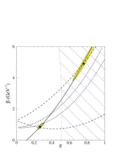
FIG. 5.: Solution contours in the $g$-$\beta$ plane for the situation in row 5 of Table I. The solid, dashed, and dotted lines correspond to solution lines for the $D^{*0}$, $D^{*+}$, and $D^{*}_{s}$ decay rate ratios respectively. The stars correspond to the minimal $\chi^{2}$ solutions and the shaded regions correspond to the 68% confidence level of experimental error in the fit. The hatched region is excluded by the experimental limit $\Gamma(D^{*+})<0.13\,{\rm MeV}$ [28].

One can see more clearly how these solutions are determined by looking at Fig. 5. The central value for each ratio of decay rates in Eq. (41) gives a possible contour in the $g$-$\beta$ plane, as shown by the solid ($D^{*0}$), dashed ($D^{*+}$), and dotted ($D_{s}^{*}$) lines. An exact solution for two of the ratios occurs at the intersection of two of these contour lines. However, a good solution for all three ratios requires a point that is close to all three lines. The solutions in the fifth row of Table I are indicated by stars in Fig. 5. The size of the experimental uncertainties can be seen in the 68% confidence level ellipses which are shown as shaded regions in the figure (for two degrees of freedom they correspond to $\chi^{2}\leq\chi^{2}_{min}+2.3$). These regions are centered on the solid line since the $D^{*0}$ ratio has the smallest experimental error. The errors in Eq. (41) give the following one sigma errors on the two solutions

$$g=0.265^{+.036}_{-.018}\ \ \ \beta=0.85^{+.21}_{-.10}\,{\rm GeV^{-1}}\>,\qquad\quad g=0.756^{+0.028}_{-0.027}\ \ \ \beta=4.90^{+.27}_{-.26}\,{\rm GeV^{-1}}\>.$$ (43)

Both solutions fit the first two ratios in Eq. (41), but do not do as well for the third. Minimizing the $\chi^{2}$ has biased against the third ratio as a result of its large experimental error. For this ratio the $g=0.265$ and $g=0.76$ solutions give values which are $4$ and $13$ times too small respectively. For the first solution it is possible to improve the fit to the third ratio with reasonably sized counterterms. For instance, simply taking $\tilde{\alpha}_{1}=2$ gives ${{\cal B}(D^{*\ }_{s}\to D_{s}\pi^{0})/{\cal B}(D^{*\ }_{s}\to D_{s}\gamma)}=0.036$. As we will see below, a large $g$ solution with $\chi^{2}\lesssim 1$ is only possible if $g$ increases to $\sim 0.9$ and $\beta$ increases to $\sim 6.0\,{\rm GeV^{-1}}$ (c.f. Fig. 6).

The experimental limit $\Gamma(D^{*+})<0.13\,{\rm MeV}$ [28] translates into an upper bound on the value of $g$. Since ${\cal B}(D^{*+}\to D^{+}\gamma)$ is small, this bound is almost $\beta$ independent and to a good approximation is

$$g<0.52\,\sqrt{\,\sqrt{1+3.01\,x}-1}\qquad\qquad x=\Gamma(D^{*+})^{\>\rm limit}/(0.13\,{\rm MeV})\,.$$ (44)

For the situation in row five of Table I this excludes the hatched region in Fig. 5. The limit on $\Gamma(D^{*+})$ therefore eliminates the $g\simeq 0.76$ solution at the two sigma level. Since this limit has not been confirmed by other groups it would be useful to have further experimental evidence that could exclude this solution.

The central values in Eq. (43) have uncertainty associated with the parameter $m_{c}$. Taking $m_{c}=1.4\pm 0.1\,{\rm GeV}$ gives $0.25<g<0.28$ and $0.79\,{\rm GeV^{-1}}<\beta<0.93\,{\rm GeV^{-1}}$ for the first solution, and $0.72<g<0.80$ and $4.6\,{\rm GeV^{-1}}<\beta<5.3\,{\rm GeV^{-1}}$ for the second solution (in both cases the $\chi^{2}$ changes very little). There is also ambiguity in the solution in Eq. (43) due to the choice of scale $\mu$ (ie., the value of the counterterms $\alpha_{1}$, $\alpha_{5}$, $\tilde{\kappa}_{1}$ and $\kappa_{5}$). Increasing $\mu$ to $1.3\,{\rm GeV}$ gives solutions $(g=0.28,\beta=0.91\,{\rm GeV^{-1}},\chi^{2}=1.4)$ and $(g=0.78,\beta=5.0\,{\rm GeV^{-1}},\chi^{2}=4.1)$, while decreasing $\mu$ to $0.7\,{\rm GeV}$ gives solutions $(g=0.25,\beta=0.83\,{\rm GeV^{-1}},\chi^{2}=3.7)$ and $(g=0.72,\beta=4.7\,{\rm GeV^{-1}},\chi^{2}=3.1)$. Note that the $\chi^{2}$ of the second solution remains large, while the $\chi^{2}$ of the first solution is reduced significantly by an increased scale.

Another method of testing the effect of the unknown counterterms $\tilde{\alpha}_{1}$, $\alpha_{5}$, $\tilde{\kappa}_{1}$ and $\kappa_{5}$ is to take their values at $\mu=1\,{\rm GeV}$ to be randomly distributed within some reasonable range of values. We take $-1<\tilde{\kappa}_{1},\kappa_{5}<1$ and $-2<\tilde{\alpha}_{1},\alpha_{5}<2$, with the motivation that the counterterms change the tree level value of $Z_{\pi}^{a}$ and $Z_{\gamma}^{a}$ by less than $30\%$, and give corrections that are not much bigger than those from the one-loop graphs. Near each of the two solutions $5000$ values of $g$ and $\beta$ were then generated by minimizing the $\chi^{2}$. This gives the distributions in Fig. 6. The solution with $g=0.265$ and $\beta=0.85\,{\rm GeV^{-1}}$ has fairly small uncertainty from the counterterms. The $g=0.76$, $\beta=4.9\,{\rm GeV^{-1}}$ solution has much larger uncertainty because the corresponding contour lines in Fig. 5 are almost parallel. For this solution the upper bounds are determined by the limits of a few ${\rm MeV}$ [13] on the $D^{*}$ widths.

FIG. 6.: Effect of the order $m_{q}$ counterterms ($\tilde{\kappa}_{1}$, $\kappa_{5}$, $\tilde{\alpha}_{1}$, and $\alpha_{5}$) on the solutions in Eq. (43). The counterterms are taken to be randomly distributed with $-1<\tilde{\kappa}_{1},\kappa_{5}<1$, $-2<\alpha_{1},\alpha_{5}<2$. For each set of counterterms $g$ and $\beta$ were determined at the new minimal $\chi^{2}$. $5000$ sets were generated near each of the two solutions.

From this analysis we estimate the theoretical uncertainty of the solutions in Eq. (43) to be roughly

$$g=0.265^{+0.05}_{-0.02}\ \ \ \beta=0.85^{+0.3}_{-0.1}\>{\rm GeV^{-1}}\>,\qquad\quad g=0.76^{+0.2}_{-0.1}\ \ \ \beta=4.9^{+5.0}_{-0.7}\>{\rm GeV^{-1}}$$ (45)

at this order in chiral perturbation theory. The errors on $g$ and $\beta$ are positively correlated since the values of $g$ and $\beta$ are constrained in one direction by the small error on the $D^{*0}$ rate ratio in Eq. (41).

From Eq. (44) and Fig. 6, we see that if the error in ${{\cal B}(D^{*\ }_{s}\to D_{s}\pi^{0})/{\cal B}(D^{*\ }_{s}\to D_{s}\gamma)}$ can be decreased by a factor of two, in conjunction with a limit of $\Gamma(D^{*+})\lesssim 0.6\,{\rm MeV}$ then this could provide strong evidence that the $g=0.76$ solution is excluded. On the other hand if the central values of the second and third ratios in Eq. (41) decrease, then a width measurement or stronger limit on $\Gamma(D^{*+})$ will be needed to distinguish the two solutions.

Using the extracted values of $g$ and $\beta$ gives the widths shown in Table II. The couplings were extracted at one-loop and order $m_{q}\sim 1/m_{c}$, so the predictions for the $D^{*}$ widths are made at this order. The experimental uncertainty in the $D^{*}$ widths is estimated by setting $g$ and $\beta$ to the extremal values in Eq. (43), which gives the range shown in the second and fourth rows of the Table. The uncertainty from the unknown counterterms in the third and fifth rows is estimated in the same way using the uncertainties from Eq. (45). Note that for the $g=0.265$ solution the $D_{s}^{*}$ width is small due to a delicate cancellation in $\mu_{3}$ resulting from setting $Z_{\rm wf}^{a}\times 1/m_{c}=1/m_{c}$. Keeping $Z_{\rm wf}^{a}/m_{c}$ to order $m_{q}$ gives a $D^{*}_{s}$ width of $0.28\,{\rm keV}$ with a range of $0.1-0.4\,{\rm keV}$ for both the experimental and the counterterm uncertainties.

Making use of HQS allows us to predict the width of the $B^{*}$ mesons from their dominant mode $B^{*}\to B\gamma$. Eq. (31) gives the rate for $B^{*}\to B\gamma$ with $Q^{\prime}=-1/3$ and $m_{c}\to m_{b}$. Since the couplings $\beta_{1}$ and $\beta_{2}$ are unknown these rates can not be determined at order $1/m_{c,b}$, but we can include the order $m_{q}$ corrections. The $B$ meson masses are taken from [13] and we use $m_{b}=4.8\,{\rm GeV}$ [27]. We set $\delta=0.047\,{\rm GeV}$  and $\Delta=k\cdot v=0$, but since the contribution $Q^{\prime}/m_{b}$ in Eq. (31) is numerically important it is kept in our estimate. For comparison the widths obtained with the $g=0.76$ and $\beta=4.9\,{\rm GeV^{-1}}$ solution are also shown.

Predicted widths in ${\rm keV}$	$D^{*0}$	$D^{*+}$	$D_{s}^{*}$	$B^{*+}$	$B^{*0}$	$B_{s}^{*}$
$g=0.265$, $\beta=0.85\,{\rm GeV^{-1}}$	18	26	0.06	$\sim$ 0.06	$\sim$ 0.03	$\sim$ 0.04
uncertainty from experiment	16 - 24	23 - 35	0.01 - 0.13	$-$	$-$	$-$
uncertainty from counterterms	16 - 27	22 - 39	0.04 - 0.13	$-$	$-$	$-$
$g=0.76$, $\beta=4.9\,{\rm GeV^{-1}}$	323	448	103	$\sim$ 2.1	$\sim$ 2.0	$\sim$ 1.6
uncertainty from experiment	285 - 367	396 - 508	83 - 1287	$-$	$-$	$-$
uncertainty from counterterms	215 - 1318	281 - 1157	53 - 1078	$-$	$-$	$-$

TABLE II.: Widths in ${\rm keV}$ for the $D^{*}$ and $B^{*}$ mesons. The experimental and counterterm ranges are determined by the extremal values of $g$ and $\beta$ in Eqs. (43) and (45). For $g=0.265$ the $D_{s}^{*}$ width is small due to a delicate cancellation in $\mu_{3}$ as explained in the text. The uncertainty in the $B^{*}$ widths is large due to unknown $1/m_{c,b}$ corrections.

As a final comment, we note that heavy meson chiral perturbation theory can also be used to examine excited $D^{(*)}$ mesons, such as the p-wave states, $D_{0}^{*}$, $D_{1}^{*}$, $D_{1}$, and $D_{2}^{*}$ [29, 11]. To do so, explicit fields for these particles may be added to the Lagrangian giving a new effective theory. For interactions without external excited mesons (such as the ones considered here) these new particles can then contribute as virtual particles. However, since we have not included these heavier particles they are assumed to be ‘integrated out’, whereby such contributions are absorbed into the definitions of our couplings.

IV Conclusion

For the $D^{*0}$, $D^{*+}$, and $D^{*}_{s}$, the decays $D^{*}\to D\pi$ and $D^{*}\to D\gamma$ are well described by heavy meson chiral perturbation theory. Using the recent measurement of ${\cal B}(D^{*+}\to D^{+}\gamma)$ [12], the ratios of the $D\gamma$ and $D\pi^{0}$ branching fractions were used to extract the $D^{*}D\pi$ and $D^{*}D\gamma$ couplings $g$ and $\beta$. Two solutions were found

$$g=0.265\,^{+.04}_{-.02}\,{}^{+.05}_{-.02}\ \ \beta=0.85^{+.2}_{-.1}\,{}^{+.3}_{-.1}\,{\rm GeV^{-1}}\,\quad\quad g=0.76\,^{+.03}_{-.03}\,{}^{+.2}_{-.1}\ \ \beta=4.9^{+.3}_{-.3}\,{}^{+5.0}_{-.7}\,{\rm GeV^{-1}}\,.$$ (46)

The first error here is the one sigma error associated with a minimized $\chi^{2}$ fit to the three experimental branching fraction ratios (see Fig. 5). The second error is our estimate of the uncertainty in the extraction due to four unknown counterterms $\tilde{\alpha}_{1}$, $\alpha_{5}$, $\tilde{\kappa}_{1}$ and $\kappa_{5}$ that arise at order $m_{q}$ (see Fig. 6).

It is possible that the uncertainty from these counterterms can be reduced by determining them from other processes. For these corrections to contribute at low enough order in the chiral expansion we need processes with outgoing photons or pseudo-goldstone bosons, such as semileptonic $D$ decays to $K$, $\eta$, or $\pi$. Here there are also SU(3) corrections to the left handed current which involve an unknown parameter $\eta_{0}$ [7]. Information on $\kappa_{1}$ and $\kappa_{1}^{\prime}$ can be determined from the pole part of the $D_{s}\to K\ell\nu_{\ell}$ form factor [7]. In a similar manner $D_{s}\to\eta\ell\nu_{\ell}$ can constrain $\tilde{\kappa}_{1}$ and $\kappa_{5}$, and a comparison of the form factors for $D^{+}\to\bar{K}^{0}\ell\nu_{\ell}$ and $D_{s}\to\eta\ell\nu_{\ell}$ gives information on $\kappa_{1}^{\prime}$ and $\kappa_{5}$. These investigations were beyond the scope of this paper. In principle, information about the constants $\tilde{\alpha}_{1}$, and $\alpha_{5}$ could be obtained from a measurement of $B\to\gamma\ell\nu_{\ell}$. The CLEO experimental bound on $B\to\ell\nu_{\ell}$ ($\ell=e,\mu$)[30] is roughly two orders of magnitude above the theoretical prediction, but due to the helicity suppression for $B\to\ell\nu_{\ell}$ the branching ratio for $B\to\gamma\ell\nu_{\ell}$ may be up to an order of magnitude bigger[31].

Another possible approach would be to use large $N_{c}$ scaling for the counterterms in $\delta{\cal L}_{g}$ and $\delta{\cal L}_{\beta}$. Terms that have two chiral traces are suppressed by a power of $N_{c}$ compared to those with only one trace. In the large $N_{c}$ limit the counterterms $\tilde{\kappa}_{1}$ and $\tilde{\alpha}_{1}$ would dominate, and $\kappa_{5}$ and $\alpha_{5}$ could be neglected, thus reducing the theoretical uncertainty.

The smaller solution for $g$ in Eq. (46) is fairly insensitive to the addition of the one-loop corrections (see Table I). However, corrections at order $m_{q}\sim 1/m_{c}$, including the heavy meson mass splittings, were important in determining the solution with larger $g$. The limit $\Gamma(D^{*+})<0.13\,{\rm MeV}$ [28] gives an upper bound on the coupling $g$ (see Eq. (44) and Fig. 5), and eliminates the $g=0.76$, $\beta=4.9\,{\rm GeV^{-1}}$ solution. Experimental confirmation of this limit is therefore desirable. Note that the largest experimental uncertainty in our extraction comes from the measurement of ${\cal B}(D_{s}^{*}\to D_{s}\pi^{0})$, and dominates the theoretical uncertainty due to decay via single photon exchange. A better measurement of ${{\cal B}(D^{*\ }_{s}\to D_{s}\pi^{0})/{\cal B}(D^{*\ }_{s}\to D_{s}\gamma)}$ along with a limit $\Gamma(D^{*+})\lesssim 0.6\,{\rm MeV}$ could provide further evidence that the $g=0.76$ solution is excluded. However, if the central values of the second and third ratios in Eq. (41) decrease then a width measurement or stronger limit on $\Gamma(D^{*+})$ will be needed to distinguish the two solutions. An improved measurement of ${\cal B}(D^{*\ }_{s}\to D_{s}\pi^{0})$ may also give valuable information on the unknown couplings $\tilde{\kappa}_{1}$, $\kappa_{5}$, $\tilde{\alpha}_{1}$, and $\alpha_{5}$.

The extraction of $g$ has important consequences for other physical quantities [2-11]. For example[32], for the $B\to\pi\ell\bar{\nu}_{\ell}$ form factors with $E_{\pi}<2\,m_{\pi}$, analyticity bounds combined with chiral perturbation theory give $g\,f_{B}\lesssim 50\,{\rm MeV}$ [33]. The solution $g=0.265$ gives $f_{B}\lesssim 190\,{\rm MeV}$ for the $B$ decay constant. However, for $g=0.76$ we have $f_{B}\lesssim 66\,{\rm MeV}$, which is roughly a factor of three smaller than lattice QCD values, $f_{B}\simeq 160-205$ [34].

Acknowledgments

I would like to thank Zoltan Ligeti and Mark B. Wise for early discussions on this subject and useful suggestions. I would also like to thank Aneesh Manohar, Tom Mehen, Vivek Sharma, Hooman Davoudiasl, and Martin Gremm for helpful comments. This work was supported in part by the U.S. Dept. of Energy under Grant no. DE-FG03-92-ER 40701.

One loop correction formulae

In this appendix we give explicit formulas for the functions $G_{1}$, $F_{1}$, $F_{2}$, $\varrho_{\pi}^{a}$, and $\varrho_{\gamma}^{a}$ that occur in our one loop correction formulae in Eqs. (17), (19), (24), and (35). In doing this type of one-loop calculation an important integral is

$$\int{d^{4-2\epsilon}q\over(2\pi)^{4-2\epsilon}}{\mu^{2\epsilon}\over(q^{2}-m^{2}+i\varepsilon)\,2(q\cdot v-b+i\varepsilon)}=-{i\,b\over(4\pi)^{2}}\left[\frac{1}{\hat{\epsilon}}+\ln{(\frac{\mu^{2}}{m^{2}})}+2-2F(\frac{m}{b})\right]\,,$$ (47)

where $1/\hat{\epsilon}=1/\epsilon-\gamma+\log{(4\pi)}$. $F$ is needed for both positive and negative $b$, so

$$F\left(\frac{1}{x}\right) = \left\{\begin{array}[]{l}-\mbox{${\sqrt{1-x^{2}}\over x}$}\left[\mbox{$\frac{\pi}{2}$}-\tan^{-1}\left(\mbox{$\frac{x}{\sqrt{1-x^{2}}}$}\right)\right]\quad\qquad|x|\leq 1\\ \phantom{-}\mbox{${\sqrt{x^{2}-1}\over x}$}\>\ln{\left(x+\sqrt{x^{2}-1}\,\right)}\quad\qquad\quad\ \ \ |x|\geq 1\end{array}\right.\,.$$ (50)

For $b>0$ the function $F$ was derived in [35, 5] and agrees with the above formula. For $x=b/m<-1$ the logarithm in Eq. (50) has an imaginary part. This corresponds to the physical intermediate state where a heavy meson of mass $m_{H}$ produces particles of mass $m_{H}+b$ and $m$. For the calculation here the imaginary part only contributes from $F(m_{\pi}/(d_{0}-\Delta))$, and was found to always be numerically insignificant. Note that the real part of $x\,F(1/x)$ is continuous everywhere, and differentiable everywhere except $x=-1$. Also $F(1)=F(-1)=0$.

Eq. (17) contains the function

$$G_{1}(a,b) = \frac{5}{3}\,a^{2}+(4b^{2}-\frac{4}{3}a^{2})F(a/b)+\frac{4}{3}(a^{2}-b^{2})\frac{a}{b}F^{\prime}(a/b)\,,$$ (51)

where $a^{2}$ is the analytic contribution. In the limit $\Delta\to 0$ Eq. (17) gives $Z_{D}=Z_{D^{*}}$ in agreement with HQS. To obtain HQS in the finite part of the dimensionally regularized calculation of the graphs in Fig. 1 it was necessary to continue the $D^{*}$ fields to $d=4-2\epsilon$ dimensions (so the $D^{*}$ polarization vector $\epsilon_{\alpha}=(1-\frac{\epsilon}{3})\tilde{\epsilon}_{\alpha}$ where $\sum\tilde{\epsilon}_{\alpha}^{\,*}\tilde{\epsilon}^{\alpha}=-3$).

In Eqs. (19) and (24) we have the functions

$$F_{1}(a,b,c) = -\frac{7}{6}\,a^{2}+\frac{2}{3(b-c)}\left[b(a^{2}-b^{2})F(a/b)-c(a^{2}-c^{2})F(a/c)\right]\,,$$ (52)

$$\varrho_{\pi}^{a=1,2} = {m_{\pi}^{2}\over(4\pi f)^{2}}{\tilde{\kappa}_{1}(\mu)\over 2}\,,$$ (53)

$$\varrho_{\pi}^{3} = {1\over(4\pi f)^{2}}\>{(m_{u}-m_{d})\over 2(m_{s}-\hat{m})}\>\bigg{[}(m_{K}^{2}-\frac{m_{\pi}^{2}}{2})\,\tilde{\kappa}_{1}+(m_{K}^{2}-m_{\pi}^{2})\,\kappa_{5}\bigg{]}+{(m_{K^{\pm}}^{2}-m_{K^{0}}^{2})\over(4\pi f)^{2}}\>\kappa_{5}\,.$$ (54)

We have ignored isospin violating counterterm corrections in $\varrho^{1,2}_{\pi}$ and work to leading order in the isospin violation for $\varrho^{3}_{\pi}$. In deriving Eq. (52) use has been made of $m_{\pi}^{2}=2B_{0}m_{u}=2B_{0}m_{d}=2B_{0}\hat{m}$, $m_{K}^{2}-m_{\pi}^{2}/2=B_{0}m_{s}$, and $m_{K^{\pm}}^{2}-m_{K^{0}}^{2}=(m_{u}-m_{d})B_{0}$.

In Eq. (35) we have the function $F_{1}$ and the function

$$F_{2}(a,b,c) = -2\,b-c-\frac{2a^{2}}{c}\int^{a/(b+c)}_{a/b}dt{F(t)\over t^{3}}$$ (55)

$$= -2\,b-c-\frac{2a^{2}}{c}\left[{1\over 4x^{2}}-{F(x)\over 2\,x^{2}}-{F(x)^{2}\over 4\,(x^{2}-1)}\right]\Bigg{|}_{x=a/b}^{x=a/(b+c)}\,.$$ (56)

Assuming isospin to be conserved the counterterm contributions in Eq. (35) are

$$\varrho_{\gamma}^{\,a=1,2} = {m_{\pi}^{2}\>\tilde{\alpha}_{1}\over 2\,(4\pi f)^{2}}\>-{(m_{K}^{2}-m_{\pi}^{2})\>\alpha_{5}\over 3\,Q_{aa}\,(4\pi f)^{2}}\,,$$ (57)

$$\varrho_{\gamma}^{3} = {(2\,m_{K}^{2}-m_{\pi}^{2})\>\tilde{\alpha}_{1}\over 2\,(4\pi f)^{2}}+{(m_{K}^{2}-m_{\pi}^{2})\>\alpha_{5}\over(4\pi f)^{2}}\,.$$ (58)

REFERENCES

• [1] N.Β Isgur and M.B.Β Wise, Phys. Lett. B232 (1989) 113; Phys. Lett. B237 (1990) 527.
• [2] C.Β Lee etΒ al. Phys. Rev. D46 (1992) 5040; H.Y.Β Cheng, etΒ al., Phys. Rev. D48 (1993) 369; G.Β Kramer, and W.F.Β Palmer, Phys. Lett. B298 (1993) 437; C.L.Y.Β Lee, Phys. Rev. D48 (1993) 2121; J.L.Β Goity and W.Β Roberts, Phys. Rev. D51 (1995) 3459.
• [3] M.B. Wise, Phys. Rev. D45, (1992) R2188; G. Burdman, and J. Donoghue, Phys. Lett. B280 (1992) 287; T.M. Yan etΒ al., Phys. Rev. D46 (1992) 1148.
• [4] N. Isgur and M.B. Wise, Phys. Rev. D41 (1990) 151; G. Burdman, etΒ al., Phys. Rev. D49 (1994) 2331; R. Fleischer, Phys. Lett. B303 (1993) 147; R. Casalbuoni etΒ al., Phys. Lett. B294, (1992) 106; Q.P. Xu, Phys. Lett. B306 (1993) 363;
• [5] A. Falk and B. Grinstein, Nucl. Phys. B416 (1994) 771.
• [6] J. Goity, Phys. Rev. D46 (1992) 3929; B. Grinstein etΒ al. Nucl. Phys. B380 (1992) 369; M. Neubert, Phys. Rev. D46 (1992) 1076; B. Grinstein, Phys. Rev. Lett. 71 (1993) 3067
• [7] C.G. Boyd and B. Grinstein, Nucl. Phys. B442 (1995) 205.
• [8] H. Davoudiasl, Phys. Rev. D54 (1996) 6830; Z. Ligeti etΒ al., hep-ph/9711248.
• [9] L.Β Randall and M.B.Β Wise, Phys.Lett. B303 (1993) 135; C.K.Β Chow and M.B.Β Wise, Phys.Rev. D48 (1993) 5202; C.G.Β Boyd and B.Β Grinstein, Nucl.Phys. B451, (1995) 177.
• [10] J.L. Rosner and M.B. Wise, Phys. Rev. D47 (1993) 343; L. Randall and E. Sather, Phys. Lett. B303 (1993) 343; E. Jenkins, Nucl. Phys. B412 (1994) 181.
• [11] R. Casalbuoni etΒ al. Phys.Rept. 281 (1997) 145.
• [12] CLEO collaboration, hep-ex/9711011.
• [13] R.M.Β Barnett et al., Phys. Rev. D54 (1996) 1; and 1997 off-year partial update for the 1998 edition available on the PDG WWW pages (URL: http://pdg.lbl.gov/).
• [14] J.L.Β Rosner, in Particles and Fields 3, Proceedings of the Banff Summer Institute, Banff Canada 1988, A.Β N.Β Kamal and F.Β C.Β Khanna, eds., World Scientific, Singapore (1989) 395; L.Β Angelos and G.Β P.Β Lepage, Phys. Rev. D45 (1992) 3021.
• [15] A.V.Β Manohar and H.Β Georgi, Nucl. Phys. B 234 (1984) 189.
• [16] P.Β Colangelo etΒ al., Phys. Lett. B334 (1994) 175; P.Β Colangelo etΒ al., Phys. Rev. D43 (1991) 3002.
• [17] V.M.Β Belyaev etΒ al. Phys. Rev. D51 (1995) 6177; P. Colangelo, etΒ al. Phys. Lett. B339 (1994) 151; T.M. Aliev etΒ al. Phys. Lett. B351 (1995) 339; and references therein.
• [18] J.F. Amundson et al., Phys. Lett. B296 (1992) 415.
• [19] P. Cho, and H. Georgi, Phys. Lett. B296, (1992) 408; Erratum-ibid B300, (1993) 410.
• [20] H.Y. Cheng et al., Phys. Rev. D49 (1994) 5857.
• [21] P. Cho, and M.B. Wise, Phys. Rev. D51 (1995) 3352.
• [22] M.Luke and A. Manohar, Phys. Lett. B286 (1992) 348.
• [23] H.Y. Cheng et al., Phys. Rev. D49 (1994) 2490.
• [24] J. Gasser and H. Leutwyler, Phys. Rept. 87 (1982) 77.
• [25] J. Gasser and H. Leutwyler, Nucl. Phys. B250 (1985) 465.
• [26] H.Y. Cheng et al., Phys. Rev. D47 (1993) 1030.
• [27] M. Gremm etΒ al., Phys. Rev. Lett. 77 (1996) 20; M. Gremm, and I. Stewart, Phys. Rev. D55 (1997) 1226.
• [28] ACCMOR Collab., S. Barlag etΒ al., Phys. Lett. B278 (1992) 480.
• [29] A. Falk, Phys. Lett. B305 (1993) 268; A. Falk and T. Mehen, Phys. Rev. D53 (1996) 231; U. Kilian etΒ al., Phys. Lett. B288 (1992) 360.
• [30] CLEO collaboration, M. Artuso etΒ al., Phys. Rev. Lett. 75 (1995) 785.
• [31] P. Colangelo etΒ al., Phys. Lett. B372 (1996) 331; G. Eilam, etΒ al., Phys. Lett. B361 (1995) 137.
• [32] Glenn Boyd and Ben Grinstein, private communication.
• [33] C.G. Boyd, et.al, Phys. Rev. Lett., 74, (1995) 4603.
• [34] A.X. El-Khadra etΒ al., hep-ph/9711426; S. Aoki etΒ al., JLQCD collaboration, hep-lat/9711041; C. Bernard, hep-ph/9709460; K-I. Ishikawa etΒ al., Phys.Rev. D56 (1997) 7028; C.R. Allton etΒ al., APE Collaboration, Phys. Lett. B405 (1997) 133; R. Baxter etΒ al., UKQCD Collaboration, Phys. Rev. D49 (1994) 1594. C.W. Bernard et al., Phys. Rev. D49 (1994) 2536.
• [35] E. Jenkins, and A.V. Manohar, Talk presented at the workshop on Effective Field Theories of the Standard Model, Dobogoko, Hungary, Aug 1991, 113.