Optimized Perturbation Theory at Finite Temperature

Abstract

An optimized perturbation theory (OPT) at finite temperature $T$, which resums higher order terms in the naive perturbation, is developed in $O(N)$ $\phi^{4}$ theory. It is proved that (i) the renormalization of the ultra-violet divergences can be carried out systematically in any given order of OPT, and (ii) the Nambu-Goldstone theorem is fulfilled for arbitrary $N$ and for any given order of OPT. The method is applied for the $O(4)$ $\sigma$ model to study the soft modes associated with the chiral transition in quantum chromodynamics. Threshold enhancement of the spectral functions at finite $T$ in the scalar and pseudo-scalar channels is shown to be a typical signal of the chiral transition.

I Introduction

One of the main goals of the ultra-relativistic heavy-ion experiments planned at RHIC and LHC [2] is to observe the structural change of the ground state of quantum chromodynamics (QCD) at finite temperature ($T$), namely the phase transition to the quark-gluon plasma. The numerical simulation based on the lattice QCD is a powerful tool to study the static nature of this phase transition, in which the critical temperature and the critical exponents are actively studied [3]. In particular, there exit numerical evidences that the chiral transition for massless two flavors is of second order, although the case for the real world (two light quarks + one medium-heavy quark) is not settled yet [4].

If the phase transition is of second order or is close to it, there arises long range fluctuations in both spatial and temporal (real-time) directions. The latter is usually called the soft mode and has been used as a probe to study phase transitions of solid states and condensed matters [5].

Despite the experimental significance of the soft modes in QCD, the lattice QCD simulations cannot treat such real-time modes in a straightforward manner. This is why effective theories of QCD have been adopted to study the time-dependent phenomena (see the reviews [6, 7] and references cited therein.) However, even in tractable effective theories such as the linear $\sigma$-model, there exist subtleties at finite $T$. In fact, the necessity of the resummation of higher order terms in perturbative expansions both at high $T$ and low $T$ has been known for a long time [8, 9]. Also, the renormalization of the ultra-violet (UV) divergences and related issue in resumed perturbation theories have been discussed in the literatures especially for theories with spontaneous symmetry breaking (SSB) [10].

Recently, we have reported our analysis of a particular resummation method and its application to the soft modes in QCD [11]. The present paper contains not only the detailed description of our previous analysis but also further investigations.

The purpose of the present paper is twofold. Firstly, we will develop an improved loop-wise expansion at finite $T$. Our starting point is the optimized perturbation theory (OPT) (or sometimes called delta-expansion, variational perturbation theory etc) which is a generalization of the mean-field method [12] and is known to work in various quantum systems [13]. Its application to field theory at finite $T$ has been considered in ref.[14, 15] for the first time. We will further develop the idea and prove the renormalizability and the Nambu-Goldstone (NG) theorem in $O(N)$ $\phi^{4}$ theory at finite $T$ order by order in OPT. Our second purpose is to study the soft modes associated with the chiral transition in QCD by taking into account interactions among the soft modes (mode couplings). The use of OPT is essential for this purpose, which will be demonstrated using the $O(4)$ $\sigma$ model.

The organization of this paper is as follows. In section II, we introduce a loop-wise expansion on the basis of OPT. The renormalization of UV divergences and the realization of the NG theorem in this method are also discussed. In section III, we will apply OPT developed in section II for the $O(4)$ $\sigma$ model to study the spectral functions of the $\sigma$-meson and the $\pi$-meson at $T\neq 0$. It is also examined the detectability of the soft modes by the diphoton process $\sigma\rightarrow 2\gamma$ in hot hadronic matter. Section IV is devoted to summary and concluding remarks.

II Optimized Perturbation at $T\neq 0$

A Necessity of resummation at finite $T$

It has been known that naive perturbations either by a coupling constant or by number of loops break down at $T\neq 0$, and proper resummation of higher orders is necessary [8]. In fact, no matter what a small dimensionless coupling (say $\lambda$) seems to control the perturbative expansion, the powers of $T$ compensate the powers of $\lambda$, which invalidates the naive expansion.

This is easily illustrated in the $\phi^{4}$ theory:

$${\cal L}={1\over 2}[(\partial\phi)^{2}-\mu^{2}\phi^{2}]-{\lambda\over 4!}\phi^{4}.$$ (1)

Let us first consider the case $\mu^{2}>0$. The lowest order self-energy diagram Fig.1 (A) is $O(\lambda T^{2})$ at high $T$. However, Fig.1 (B) is $O(\lambda T^{2}\times{\lambda T\over\mu})$. Furthermore, higher powers of $T/\mu$ arise in higher loops; e.g. the n-loop diagram in Fig.1 (C) is $O(\lambda^{n}T^{2n-1}/\mu^{2n-3})$. Thus, one should at least resum cactus diagrams to get sensible results at high $T$ [8, 16]. Physics behind this resummation is of course the Debye screening mass in the hot plasma.

The naive loop-expansion breaks down also for $\mu^{2}<0$. The tree-level mass $m_{0}$ in this case is defined as

$$m_{0}^{2}=\mu^{2}+{\lambda\over 2}\xi^{2}(T),$$ (2)

where $\xi(T)$ is the thermal expectation value of $\phi$. Since $\mu^{2}$ is negative and $\xi^{2}$ decreases as $T$ increases, $m_{0}^{2}$ becomes tachyonic even below the critical temperature $T_{c}$. Therefore, the naive loop-expansion using the tree-level propagator ceases to work even before the symmetry restoration takes place, and proper resummation of higher loop diagrams is necessary [9]. Note that, for $T<T_{c}$, there is no reason to believe that only the cactus diagrams shown in Fig.1 are dominant; there exists a three-point vertex $\lambda\xi\phi^{3}$ which is not negligible for $T\sim\xi(T)$.

B Resummation method

For theories without SSB, a systematic resummation method to obtain a sensible “ weak-coupling” expansion at high $T$ was formulated and applied to gauge theory and $\phi^{4}$ theory successfully [17].

For theories with SSB, however, loop-expansion rather than the weak-coupling expansion is relevant, since one needs to treat the thermal effective potential or the Gibbs free energy. We find that the optimized perturbation theory (OPT), which was applied to finite $T$ system in [14, 15], can be formulated in such a way that an improved loop-expansion is carried out systematically. Also, the method leads to a transparent renormalization procedure and guarantees the Nambu-Goldstone theorem order by order in the improved loop-expansion.

In the following, we divide our resummation procedure into three steps and apply it to the $\phi^{4}$ theory. The case for $O(N)$ $\phi^{4}$ theory will be discussed in Section II.E.

Step 1:
Start with a renormalized Lagrangian with counter terms

$${\cal L}(\phi;\mu^{2}) = {1\over 2}[(\partial\phi)^{2}-\mu^{2}\phi^{2}]-{\lambda\over 4!}\phi^{4}$$ (4)

$$+{1\over 2}A(\partial\phi)^{2}-{1\over 2}B\mu^{2}\phi^{2}-{\lambda\over 4!}C\phi^{4}+D\mu^{4}.$$

Here we have explicitly written the argument $\mu^{2}$ in ${\cal L}$ for later use. The mass independent renormalization scheme with the dimensional regularization is assumed in (4). Just for notational simplicity, the factor $\kappa^{(4-n)}$ to be multiplied to $\lambda$ is omitted ($\kappa$ is the renormalization point and $n$ is the number of dimensions). In the actual calculations below, we take the modified minimal subtraction ($\overline{MS}$) scheme.

The $c$-number counter term $D\mu^{4}$, which was not considered in [15], is necessary to make the thermal effective potential finite. Also, it plays a crucial role for renormalization in OPT as will be shown in Sec.II.D.

The thermal effective action $\Gamma[\varphi^{2}]$ is written as the Euclidean functional integral [18]

$${\Gamma[\varphi^{2}]}=\ln\int[d\phi]\exp\left[{1\over\delta}\int_{0}^{1/T}d^{4}x\left[{\cal L}(\phi+\varphi;\mu^{2})+J\phi\right]\right],$$ (5)

where $J\equiv-\partial\Gamma[\varphi]/\partial\varphi$ and $\int_{0}^{1/T}d^{4}x\equiv\int_{0}^{1/T}d\tau\int d^{3}x$. The “naive” loop expansion at $T\neq 0$ is defined as an expansion by $\delta$ [19] with the tree-level mass $\mu^{2}+\lambda\varphi^{2}/2$.

Under the naive loop-expansion with (4) for $\mu^{2}>0$, one can completely fix the renormalization constants. Since ultra-violet (UV) divergences do not dependent on $T$ in the naive loop-expansion [20], $A,B$, $C$ and $D$ are independent of $T$, and are expanded as

$$\left(\begin{array}[]{c}A\\ B\\ C\\ D\end{array}\right)=\sum_{l=1}^{\infty}\left(\begin{array}[]{c}a_{l}\\ b_{l}\\ c_{l}\\ d_{l}\end{array}\right)\delta^{l}.$$ (14)

The coefficients ($a_{l},b_{l},c_{l},d_{l}$) are independent of $\mu^{2}$, since we use the mass independent renormalization scheme. Also, the UV divergences in the symmetry broken phase $(\mu^{2}<0)$ can be removed by the same counter terms determined for $\mu^{2}>0$ [21, 22].

The relations of $A,B,C$ and $D$ with the standard renormalization constants are $A=Z-1$, $B=Z_{\mu}Z-1$ and $C=Z_{\lambda}Z^{2}-1$, where $Z$’s are defined by $\phi_{0}=\sqrt{Z}\phi$, $\lambda_{0}=Z_{\lambda}\lambda$ and $\mu_{0}^{2}=Z_{\mu}\mu^{2}$ with suffix $0$ indicating unrenormalized quantities.

Step 2:
Rewrite the Lagrangian (4) by introducing a new mass parameter $m^{2}$ following the idea of OPT [13]:

$$\mu^{2}=m^{2}-(m^{2}-\mu^{2})\equiv m^{2}-\chi.$$ (15)

This identity should be used not only in the standard mass term but also in the counter terms [23], which is crucial to show the order by order renormalization in OPT:

$${\cal L}(\phi;\mu^{2}) = {\cal L}_{\rm r}+{\cal L}_{\rm c}$$ (16)

$${\cal L}_{\rm r} = {1\over 2}[(\partial\phi)^{2}-m^{2}\phi^{2}]-{\lambda\over 4!}\phi^{4}+{1\over 2}\chi\phi^{2}$$ (17)

$${\cal L}_{\rm c} = {1\over 2}A(\partial\phi)^{2}-{1\over 2}B(m^{2}-\chi)\phi^{2}-{\lambda\over 4!}C\phi^{4}$$ (19)

$$+D(m^{2}-\chi)^{2}.$$

$A$, $B$, $C$ and $D$ in ${\cal L}_{\rm c}$ were already determined in Step 1.

On the basis of eq.(16), we define a “modified” loop-expansion in which the tree-level propagator has a mass $m^{2}+\lambda\varphi^{2}/2$ instead of $\mu^{2}+\lambda\varphi^{2}/2$. Major difference between this expansion and the naive one is the following assignment

$$m^{2}=O(\delta^{0}),\ \ \ \ \chi=O(\delta).$$ (20)

The physical reason behind this assignment is the fact that $\chi$ reflects the effect of interactions. If one adopts an assignment, $m^{2}=O(\delta^{0}),\chi=O(\delta^{0})$, the modified loop-expansion immediately reduces to the naive one.

As will be shown explicitly in Sec. II.D, all the UV divergences in the modified loop-expansion are removed by the counter terms determined in the naive loop-expansion.

Since (16) is simply a reorganization of the Lagrangian, any Green’s functions (or its generating functional) calculated in the modified loop-expansion should not depend on the arbitrary mass $m$ if they are calculated in all orders. However, one needs to truncate perturbation series at certain order in practice. This inevitably introduces explicit $m$ dependence in Green’s functions. Procedures to determine $m$ are given in Step 3 below.

To find the ground state of the system, one should look for the stationary point of the thermal effective potential $V(\varphi^{2})$ defined by

$$V(\varphi^{2})=-{\Gamma[\varphi^{2}={\rm const.}]\over\int_{0}^{1/T}d^{4}x}.$$ (21)

As mentioned above, $V$ calculated up to $L$-th loops $V_{L}(\varphi^{2};m)$ has explicit $m$-dependence. Thus the stationary condition reads

$${\partial V_{L}(\varphi^{2};m)\over\partial\varphi}=0,$$ (22)

where derivative with respect to $\varphi$ does not act on $m$ by definition. Eq.(22) gives a stationary point of $V_{L}$ for given $m$.

One may generalize Step 2 by adding and subtracting $\alpha_{0}(\partial_{0}\phi)^{2}$, $\alpha_{1}(\partial_{i}\phi)^{2}$ and $\gamma\phi^{4}$ [24] with $\alpha_{0}$, $\alpha_{1}$ and $\gamma$ being finite parameters to be determined by the PMS or FAC conditions (see Step 3). $\alpha_{0}$ and $\alpha_{1}$ are especially important for theories with fermions at finite $T$ and chemical potential [25]. We will, however, concentrate on the simplest version ($\alpha_{0,1}=\gamma=0$) in the following discussions.

Step 3:
The final step is to find an optimal value of $m$ by imposing physical conditions à la Stevenson [26] such as the following.

• The principle of minimal sensitivity (PMS): this condition requires that a chosen quantity calculated up to $L$-th loops (${\cal O}_{L}$) should be stationary by the variation of $m$:

  $${\partial{\cal O}_{L}\over\partial m}=0.$$ (23)

• The criterion of the fastest apparent convergence (FAC): this condition requires that the perturbative corrections in $O_{L}$ should be as small as possible for a suitable value of $m$.

  $${\cal O}_{L}-{\cal O}_{L-n}=0,$$ (24)

  where $n$ is chosen in the range, $1\leq n\leq L$.

The above conditions reduce to self-consistent gap equations whose solution determine the optimal parameter $m$ for given $L$. Thus $m$ becomes a non-trivial function of $\varphi$, $\lambda$ and $T$ [27]. This together with the solution of (22) completely determine the thermal expectation value $\xi(T)\equiv\langle\phi\rangle$ as well as the optimal parameter $m(T)$. Through this self-consistent process, higher order terms in the naive loop expansion are resumed.

The choice of ${\cal O}_{L}$ in Step 3 depends on the quantity one needs to improve most. To study the static nature of the phase transition, the thermal effective potential $V_{L}(\varphi^{2};m)$ is most relevant. Applying the PMS condition for $V_{L}$ reads

$${\partial V_{L}(\varphi^{2};m)\over\partial m}=0,$$ (25)

which gives a solution $m=m(\varphi)$. This can be used to improve the effective potential at finite $T$ [14];

$$V_{L}(\varphi^{2};m)\rightarrow V_{L}(\varphi^{2};m(\varphi)).$$ (26)

Also, $\xi(T)$ and $m(T)$ are obtained by solving (22) together with (25). In this case, the following relation holds: ${dV(\varphi^{2};m(\varphi))/d\varphi}|_{\varphi=\xi}={\partial V(\varphi^{2};m(\varphi))/\partial\varphi}|_{\varphi=\xi}$.

To improve particle properties at finite $T$, it is more efficient to apply PMS or FAC conditions directly to the two-point functions [28]. In ref.[15], FAC with $L=n=2$ was used for the boson self-energy calculated up to two-loops. We will adopt a similar condition in Sec.III when we analyze spectral functions of the soft modes.

C UV divergence in the resumed perturbation

We briefly mention here the reason why the renormalization in resumed perturbation is not a trivial issue.

In the naive perturbation theory, there arises no new UV divergences at $T\neq 0$ because of the natural cutoff from the Boltzmann distribution function. Therefore, all the UV divergences at finite $T$ are canceled by the counter terms prepared at $T=0$. This statement has been proved in imaginary-time and real-time formalisms [20].

On the other hand, in self-consistent methods at $T\neq 0$, the situation is not so simple since the tree-level propagators have $T$-dependent mass (such as $m(T)$ in the above) which contains higher loop contributions through the self-consistent gap-equation [10].

In fact, in most of the self-consistent methods applied so far (except for ref.[15]), the renormalization is taken into account “after” imposing the gap-equation. This procedure not only makes the renormalization non-trivial and hard in higher orders, but also obscures the origin of the UV divergences. On the contrary, in OPT explained in the previous subsection, the renormalization is performed “before” imposing the gap-equation. In other words, the UV divergences are already removed in Step 2, and a “finite” gap-equation is obtained from the outset in Step 3.

D Renormalization in OPT

We now prove the order by order renormalization in OPT. Let us first rewrite eq.(16) as

$${\cal L}(\phi;\mu^{2}) = {\cal L}(\phi;m^{2})$$ (28)

$$+{1\over 2}\chi\phi^{2}+\left[{1\over 2}B\chi\phi^{2}+D\chi^{2}-2Dm^{2}\chi\right].$$

Since we use the symmetric and mass independent renormalization scheme (such as the $\overline{MS}$ scheme), any Green’s function generated by ${\cal L}(\phi;m^{2})$ can be renormalized solely by the coefficients $A$, $B$, $C$ and $D$ in ${\cal L}(\phi;\mu^{2})$.

Suppose we make a multiple insertion of the composite operator $(1/2)\chi\phi^{2}$ to the Green’s function generated by ${\cal L}(\phi;m^{2})$. The question is whether new divergences induced by the operator insertion are made finite only by the last three counter terms in (28). (Note that $B$ and $D$ are already fixed in Step 1, and we do not have any freedom to change them.)

The above problem is obviously related to the renormalization of composite operators. In fact, the standard method [30] tells us that necessary counter terms to remove the divergences induced by the insertion of $(1/2)\chi\phi^{2}$ are written as

$${1\over 2}(ZZ^{-1}_{\phi^{2}}-1)\chi\phi^{2}+\Delta_{2}\chi^{2}+\Delta_{1}\chi.$$ (29)

Here $Z_{\phi^{2}}$ is the renormalization constant for the composite operator $\phi^{2}$, and is necessary to remove the divergence in Fig. 2(A). $\Delta_{2}$ and $\Delta_{1}$ are necessary to remove the overall divergences in Fig. 2(B) and in Fig. 2(C), respectively.

Now, one can prove that (29) coincides with the last three terms in (28):

$$ZZ^{-1}_{\phi^{2}}-1=B,\ \ \ \Delta_{2}=D,\ \ \ {\rm and}\ \ \ \Delta_{1}=-2Dm^{2}.$$ (30)

The first equation is obtained by the definition $B=Z_{\mu}Z-1$ and an identity

$$Z_{\phi^{2}}=Z_{\mu}^{-1}.$$ (31)

The overall divergence of the vacuum diagram with no external-legs is removed by the $c$-number counter term $Dm^{4}$ in ${\cal L}(\phi;m^{2})$. Therefore, the last two equations in (30) are obtained as

$$\Delta_{1} = -({\partial\over\partial m^{2}})\left[Dm^{4}\right]=-2Dm^{2},$$ (32)

$$2\Delta_{2} = ({\partial\over\partial m^{2}})^{2}\left[Dm^{4}\right]=2D.$$ (33)

For completeness, an explicit proof of (31,32,33) is given in APPENDIX A.

Eq.(30) shows clearly that all the necessary counter terms in OPT are supplied solely by the original Lagrangian ${\cal L}(\phi;\mu^{2})$. Let us now define $\chi^{j}\Gamma^{(n,j)}_{R}(\lambda,m^{2})$ as a renormalized $n$-point proper vertex with insertion of $(1/2)\chi\phi^{2}$ by $j$-times. (Here the external momentums are not written explicitly.) The counter terms in (29) together with (30) assure the finiteness of $\Gamma^{(n,j)}_{R}$. Since the proper vertex can be expanded as $\chi^{j}\Gamma^{(n,j)}_{R}=\delta^{j}\sum_{l=0}^{\infty}\gamma_{l}\delta^{l}$, each coefficient $\gamma_{l}$ is also finite. This implies that $\chi^{j}\Gamma^{(n,j)}_{R}$ can be made finite order by order in OPT.

Three comments are in order here:

• Because the renormalization is already carried out in Step 2, one obtains finite gap-equations from the beginning in Step 3. Our procedure “resummation after renormalization” has several advantages over the conventional procedure “resummation before renormalization” where UV divergences are hoped to be canceled after imposing the gap-equation. The difference between the two is prominent especially in higher order calculations.

• The decomposition (15) should be done both in the mass term and the counter terms. This guarantees the order by order renormalization in our modified loop-expansion. In ref.[15], the order by order renormalization was checked up to the two-loop order in the $\phi^{4}$ theory at high $T$. Our proof shows that this nice feature holds in any higher orders in OPT. On the other hand, if one keeps the original counter term $(1/2)B\mu^{2}\phi^{2}+D\mu^{4}$ without the decomposition (15), $L$-loop diagrams with $L>M$ must be taken into account to remove the UV divergences in the $M$-loop order (see e.g. the last reference in [17]). This is an unnecessary complication due to the inappropriate treatment of the counter terms.

• As far as we stay in the low energy region far below the Landau pole, we need not address the issue of the triviality of the $\phi^{4}$ theory [29]: Perturbative renormalization in OPT works in the same sense as that in the naive perturbation.

E Nambu-Goldstone theorem

The procedure and the renormalization in OPT discussed above do not receive modifications even if the Lagrangian has global symmetry. For $O(N)$ $\phi^{4}$ theory, one needs to replace $\phi$ and $\phi^{2}$ by $\vec{\phi}=(\phi_{0},\phi_{1},\cdot\cdot\cdot,\phi_{N-1})$ and $\vec{\phi}^{2}$ respectively in all the previous formulas. In the symmetry broken phase of such theory, the Nambu-Goldstone (NG) theorem and massless NG bosons are guaranteed in each order of the modified loop-expansion in OPT for arbitrary $N$. To show this, it is most convenient to start with the thermal effective potential $V(\vec{\varphi}^{2})$. By the definition of the effective potential, $V(\vec{\varphi}^{2})$ has manifest $O(N)$ invariance if it is calculated in all orders.

In OPT, $V$ calculated up to $L$-th loops $V_{L}(\vec{\varphi}^{2};m)$ has also manifest $O(N)$ invariance, because our decomposition (15) used in (16) does not break $O(N)$ invariance. Once $V_{L}$ has invariance under the $O(N)$ rotation ($\varphi_{i}\rightarrow\varphi_{i}+i\theta^{a}T^{a}_{ij}\varphi_{j}$), the immediate consequence is the standard identity:

$${\partial V_{L}(\vec{\varphi}^{2};m)\over\partial\varphi_{j}}T_{ji}^{a}=-{\partial^{2}V_{L}(\vec{\varphi}^{2};m)\over\partial\varphi_{i}\partial\varphi_{j}}T_{jk}^{a}\varphi_{k},$$ (34)

with ${\bf T}^{a}$ being the generator of the $O(N)$ symmetry. Eq.(34) is valid for arbitrary $L$, $m$ and $N$.

At the stationary point where the l.h.s. of (34) vanishes, there arises massless NG bosons for $T_{jk}^{a}\varphi_{k}\neq 0$, since the r.h.s. of (34) is equal to $-{\cal D}_{ij}^{-1}(0)T_{jk}^{a}\phi_{k}$ where ${\cal D}_{ij}(0)$ is the Matsubara propagator at zero frequency and momentum calculated up to $L$-th loops. Thus the existence of the NG bosons is proved independent of the structure of the gap-equation in Step 3.

It is instructive here to show some unjustified approximations which lead to the breakdown of the NG theorem. Many of the self-consistent methods applied so far suffer from these problems [31].

1. Suppose one takes into account only a part of the diagrams for given number of loops. Then the pion is no longer massless even if the symmetry is spontaneously broken. Although this is a trivial point, sometimes such approximation is adopted in the literatures: taking only the self-energy from the four-point vertex and neglecting that from the three-point vertex is a typical example.

2. Introducing $m^{2}$ in the $O(N)$ symmetric way as (15) is a key for the NG theorem to hold in each order of the loop-expansion in OPT. Suppose that we make a general decomposition such as

   $$\mu^{2}\delta_{ij}=m^{2}_{ij}-(m^{2}_{ij}-\mu^{2}\delta_{ij}),$$ (35)

   with $m^{2}_{ij}\neq m^{2}\delta_{ij}$. This leads to an $O(N)$ non-invariant effective potential, and the relation (34) is not guaranteed in any finite orders of the loop-expansion. For example, when the $O(N)$ symmetry is spontaneously broken down to $O(N-1)$, one may be tempted to make a decomposition $m_{ij}^{2}=m_{0}^{2}$ ($i$=$j$=0), $m_{ij}^{2}=m_{1}^{2}$ ($i$=$j$$\neq$0), and $m_{ij}^{2}=0$ ($i$$\neq$$j$). This leads to an effective potential $V_{L}(\varphi_{0}^{2},\sum_{i=1}^{N-1}\varphi_{i}^{2};m_{0},m_{1})$ which has only $O(N-1)$ invariance. It implies that eq.(34) hold only for generators which do not mix $\varphi_{0}$ with $\varphi_{i\neq 0}$. However, eq.(34) for those generators alone are not enough to prove the existence of NG bosons: In fact, $\varphi_{k\neq 0}$ in the r.h.s. of (34) vanishes in the $O(N-1)$ symmetric ground state, and no constraints are obtained for ${\cal D}_{ij}^{-1}(0)$.

III Application to $O(4)$ $\sigma$ model

Let us apply OPT to study the soft mode associated with chiral transition. Our main goal is to investigate the spectral functions of the soft modes at finite $T$:

$$\rho_{\phi}(\omega,{\bf k};T)=-{1\over\pi}\mbox{Im}D_{\phi}^{R}(\omega,{\bf k};T).$$ (36)

Here $D_{\phi}^{R}$ is the retarded correlation function

$$D_{\phi}^{R}(\omega,{\bf k};T)=-i\int d^{4}xe^{ikx}\theta(t)\langle[\phi(t,{\bf x}),\phi(0,{\bf 0})]\rangle,$$ (37)

where $\langle\cdot\rangle$ denotes thermal expectation value, and $\phi(t,{\bf x})$ is $\bar{q}q(t,{\bf x})$ or $\bar{q}i\gamma_{5}\vec{\tau}q(t,{\bf x})$ in QCD.

This spectral function was first studied using the Nambu-Jona-Lasinio model of QCD in the large $N_{c}$ limit [32]. The analysis shows that the scalar meson $\sigma$, which has a large width due to the strong decay $\sigma\rightarrow 2\pi$, decreases its mass as $T$ increases. Eventually, $\sigma$ shows up as a sharp resonance near the critical point of chiral transition. The detectability of such resonance was studied in the context of the ultra-relativistic heavy ion collisions [33]. Also, the spectral integrals in QCD at finite $T$ were studied using the operator product expansion [34].

In the following, we will adopt a toy model ($O(4)$ linear $\sigma$ model) to study the effect of mode couplings (interaction among the soft modes) in the one-loop level at finite $T$. This model shares common symmetry and dynamics with QCD and has been used to study the real-time dynamics and critical phenomena [35, 36].

A Determination of the parameters at $T=0$

The $O(4)$ $\sigma$ model reads

$${\cal L} = {1\over 2}[(\partial\vec{\phi})^{2}-\mu^{2}\vec{\phi}^{2}]-{\lambda\over 4!}(\vec{\phi}^{2})^{2}+h\sigma$$ (39)

$$\mbox{}+{1\over 2}A(\partial\vec{\phi})^{2}-{1\over 2}B\mu^{2}\vec{\phi}^{2}-{\lambda\over 4!}C(\vec{\phi}^{2})^{2}+D\mu^{4},$$

with $\vec{\phi}=(\sigma,\vec{\pi})$. $h\sigma$ is an explicit chiral symmetry breaking term [37]. $A$, $B$, $C$ and $D$ in the one-loop order are

$$A=0,\ \ \ B={\lambda\over 16\pi^{2}}{1\over\bar{\varepsilon}},\ \ \ C={\lambda\over 8\pi^{2}}{1\over\bar{\varepsilon}},\ \ \ D=-{1\over 16\pi^{2}}{1\over\bar{\varepsilon}},$$ (40)

where ${1\over\bar{\varepsilon}}\equiv{2\over 4-n}-\gamma+\log(4\pi)$, with $\gamma$ being the Euler constant.

When SSB takes place $(\mu^{2}<0)$, the replacement $\sigma\rightarrow\sigma+\xi$ in eq.(39) leads to the tree-level masses of $\sigma$ and $\pi$;

$$m_{0\sigma}^{2}=\mu^{2}+\frac{\lambda}{2}\xi^{2},\ \ m_{0\pi}^{2}=\mu^{2}+\frac{\lambda}{6}\xi^{2}.$$ (41)

The expectation value $\xi$ at $T=0$ is determined by the stationary condition for the standard effective potential $\partial V(\vec{\varphi})/\partial\varphi_{j}=0$.

Later we will take a special FAC condition in which $m^{2}$ deviates from $\mu^{2}$ only at $T\neq 0$, so that the naive loop-expansion at $T=0$ is valid. The renormalized couplings $\mu^{2},\lambda$ and $h$ can thus be determined by the following physical conditions in the naive loop-expansion at zero $T$:

1. On-shell condition for the pion $D_{\pi}^{-1}(k^{2}=m_{\pi}^{2})=0$, where $m_{\pi}=140$ MeV, and $D_{\pi}$ is the causal propagator for the pion in one-loop order.

2. Partially conserved axial-vector current (PCAC) relation in one-loop; $f_{\pi}m_{\pi}^{2}=h\sqrt{Z_{\pi}}$. Here $f_{\pi}=93$ MeV, and $Z_{\pi}$ is the finite wave function renormalization constant for the pion on its mass-shell.

3. The peak position of the spectral function in the $\sigma$ channel ($\equiv m^{peak}_{\sigma}$) is taken to be 550 MeV, 750 MeV or 1000 MeV.

$m^{peak}_{\sigma}=$ 550 MeV in (iii) is consistent with recent re-analyses of the $\pi$-$\pi$ scattering phase shift [38]. However, our main conclusions do not suffer qualitative change by other choices, 750 MeV and 1000 MeV. Instead of $m_{\sigma}^{peak}$, one may take the $\pi$-$\pi$ scattering phase shift itself as a condition to determine parameters [35]. However, for the discussions in the following, such sophistication is not necessary.

We still have a freedom to choose the renormalization point $\kappa$. Instead of trying to determine optimal $\kappa$ by the renormalization group equation for the effective potential [39], we take a simple and physical condition $m_{0\pi}$=$m_{\pi}$=140 MeV which is suitable for our later purpose. This choice has two advantages: (a) The one-loop pion self-energy $\Sigma_{\pi}(k^{2})$ vanishes at the tree-mass; $\Sigma_{\pi}(k^{2}=m_{0\pi}^{2})=\Sigma_{\pi}(k^{2}=m_{\pi}^{2})=0$, where we have used the condition (i) together with $m_{0\pi}=m_{\pi}$. (b) The spectral function in the $\sigma$ channel starts from a correct continuum threshold in the one-loop level. (In the loop-expansion, $\rho_{\sigma}(\omega,{\bf 0})$ has a physical threshold at $\omega=2m_{\pi}$=280 MeV only if $m_{0\pi}=m_{\pi}$.)

Resultant parameters are summarized in TABLE I. The spectral functions $\rho_{\sigma}$ and $\rho_{\pi}$ defined in (36) at $T=0$ with $s\equiv\omega^{2}-{\bf k}^{2}$ are shown in Fig. 3. In the $\pi$ channel, there are one particle pole and a continuum starting from the threshold $\sqrt{s_{th}}=m_{0\pi}+m_{0\sigma}$. $\sqrt{s_{th}}$ is the point where the channel $\pi+\sigma$ opens. In the $\sigma$ channel, the spectral function starts from the threshold $2m_{0\pi}=280$ MeV and shows a broad peak centered around $\sqrt{s}=m^{peak}_{\sigma}$. The half width of the peak is 260 MeV, 657 MeV and 995 MeV for $m_{\sigma}^{peak}=$ 550 MeV, 750 MeV and 1000 MeV, respectively. The large width of $\sigma$ is due to a strong $\sigma$-$2\pi$ coupling in the linear $\sigma$ model. The corresponding $\sigma$-pole is located far from the real axis on the complex $s$ plane.

B Application of OPT

Now let us proceed to Step 2 in OPT and rewrite eq.(39) as

$${\cal L} = {1\over 2}[(\partial\vec{\phi})^{2}-m^{2}\vec{\phi}^{2}]-{\lambda\over 4!}(\vec{\phi}^{2})^{2}+{1\over 2}\chi\vec{\phi}^{2}+h\sigma$$ (43)

$$-{1\over 2}Bm^{2}\vec{\phi}^{2}-{\lambda\over 4!}C(\vec{\phi}^{2})^{2}+Dm^{4}.$$

Since $\chi$ ( = $m^{2}-\mu^{2}$) is already a one-loop order, we have neglected the terms proportional to $B\chi$, $D\chi^{2}$ and $D\chi$ which are two-loop or higher orders.

When SSB takes place ($\sigma\rightarrow\sigma+\xi$), the tree-level masses to be used in the modified loop-expansion read

$$m_{0\sigma}^{2}=m^{2}+\frac{\lambda}{2}\xi^{2},\ \ m_{0\pi}^{2}=m^{2}+\frac{\lambda}{6}\xi^{2}.$$ (44)

Since $m^{2}$ will eventually be a function of $T$, the tree-masses running in the loops are not necessary tachyonic at finite $T$ contrary to the naive loop-expansion (see the discussion in Sec. II.A).

The thermal effective potential $V(\vec{\varphi};m)$ is calculated in the standard manner except for the extra terms proportional to $\chi$. The Gibbs free energy $G(\xi;m)\equiv V(\vec{\varphi}=(\xi,{\bf 0});m)$ in the one-loop level reads

$$G(\xi;m)=$$ (45)

$${1\over 2}\mu^{2}\xi^{2}+{\lambda\over 4!}\xi^{4}-h\xi$$ (46)

$$+{1\over 64\pi^{2}}\left[m_{0\sigma}^{4}\ {\rm ln}\left|{m_{0\sigma}^{2}\over\kappa^{2}e^{3/2}}\right|+3m_{0\pi}^{4}\ {\rm ln}\left|{m_{0\pi}^{2}\over\kappa^{2}e^{3/2}}\right|\right]$$ (47)

$$+T\int{d^{3}k\over(2\pi)^{3}}\left[{\rm ln}(1-e^{-E_{\sigma}/T})+3\ {\rm ln}(1-e^{-E_{\pi}/T})\right],$$ (48)

where $E_{\phi}\equiv\sqrt{{\bf k}^{2}+m_{0\phi}^{2}}$. Although this has the similar structure with the standard free energy in the naive loop-expansion, the coefficient of the first term in the r.h.s. of (45) is $\mu^{2}$ instead of $m^{2}$. This is because we have extra mass-term proportional to $\chi$ in the one-loop level. The stationary point $\xi$ is obtained by

$$\left.{\partial V(\vec{\varphi};m)\over\partial\varphi_{i}}\right|_{\vec{\varphi}=(\xi,{\bf 0})}={\partial G(\xi;m)\over\partial\xi}=0.$$ (49)

Since the derivative with respect to $\xi$ does not act on $m$, this gives a solution $\xi$ as a function of $T$ and $m$. By imposing another condition on $m$ (Step 3), one eventually determines both $\xi$ and $m$ for given $T$.

At finite $T$, the retarded propagator has a general form

$$iD^{R}_{\phi}(\omega,{\bf k};T)={i\over k^{2}-m_{0\phi}^{2}-\Sigma^{R}_{\phi}(\omega,{\bf k};T)},$$ (50)

with $k^{2}=\omega^{2}-{\bf k}^{2}$. The spectral function is then written as

$$\rho_{\phi}(\omega,{\bf k};T)=-{1\over\pi}\ {{\rm Im}\Sigma^{R}_{\phi}\over(k^{2}-m_{0\phi}^{2}-{\rm Re}\Sigma^{R}_{\phi})^{2}+({\rm Im}\Sigma^{R}_{\phi})^{2}}.$$ (51)

The retarded self-energy $\Sigma^{R}_{\phi}$ is related to the 11-component of the 2 $\times$ 2 self-energy in the real-time formalism [40];

$${\rm Re}\Sigma^{R}_{\phi}(\omega,{\bf k};T) = {\rm Re}\{\Sigma^{11}_{\phi}(\omega,{\bf k})+\Sigma^{11}_{\phi}(\omega,{\bf k};T)\}$$ (52)

$${\rm Im}\Sigma^{R}_{\phi}(\omega,{\bf k};T) = \tanh({\omega\over 2T})\ {\rm Im}\{\Sigma^{11}_{\phi}(\omega,{\bf k})+\Sigma^{11}_{\phi}(\omega,{\bf k};T)\}.$$ (53)

Here $\Sigma^{11}_{\phi}(\omega,{\bf k};T)$ is defined as a part with explicit $T$-dependence through the Bose-Einstein distribution, while $\Sigma^{11}_{\phi}(\omega,{\bf k})$ is the part which has only implicit $T$-dependence through $m(T)$ and $\xi(T)$. In the one-loop level, $\Sigma^{11}_{\phi}$ can be calculated only by the 11-component of the free propagator,

$$iD_{0\phi}^{11}(k^{2};T)={i\over k^{2}-m_{0\phi}^{2}+i\epsilon}+2\pi n_{B}\delta(k^{2}-m_{0\phi}^{2}),$$ (54)

with $n_{B}=[e^{\omega/T}-1]^{-1}$.

One-loop diagrams in OPT for $\Sigma^{11}_{\phi}$ are shown in Fig. 4. Their explicit forms are given in APPENDIX B. The NG theorem discussed in Sec.II.E can be explicitly checked by comparing eq.(49) and the inverse pion-propagator at zero momentum $[D^{R}_{\pi}(0,{\bf 0};T)]^{-1}$.

C Cancellation of $T$-dependent infinities

It is instructive here to show explicitly how the UV divergences discussed in Sec.II.D are canceled in the one-loop order. The divergent part of $\Sigma_{\pi}^{R}(\omega,{\bf k};T)$ from diagrams Fig.4($h,i,j$) reads

$$\Sigma_{\pi}^{R}[(h)+(i)+(j)]$$ (55)

$$\rightarrow -{\lambda\over 16\pi^{2}\bar{\varepsilon}}\left({5\over 6}m_{0\pi}^{2}(T)+{1\over 6}m_{0\sigma}^{2}(T)+{\lambda\xi^{2}(T)\over 9}\right)$$ (58)

$$=-{\lambda\over 16\pi^{2}\bar{\varepsilon}}\left(m^{2}(T)+{1\over 3}\lambda\xi^{2}(T)\right)$$

$$=-\Sigma_{\pi}^{R}[(l)+(m)],$$

where eq.(44) has been used. Namely, the terms proportional to $m^{2}(T)$ in Fig.4($h,i)$ are canceled by the counter term proportional to $Bm^{2}$, while the terms proportional to $\xi^{2}(T)$ in Fig.4($h,i,j)$ are canceled by the usual counter terms proportional to $C$. In this way, the $T$-dependent divergences proportional to $m^{2}(T)$ newly appeared in OPT is automatically canceled by the $T$-dependent counter terms obtained by the shift $\mu^{2}=m^{2}-\chi$. The divergence of the free energy proportional to $m^{4}$ is also canceled by the last counter term in (28).

Note that the divergences proportional to $\chi$ start to appear from the two-loop level. They are removed by the counter terms proportional to $\chi$ obtained by the shift $\mu^{2}=m^{2}-\chi$.

D FAC condition for $m^{2}$

Since we are interested in the spectral functions in the one-loop level, a best way to determine $m^{2}$ is to use the two point function in the $\pi$ channel. In [15], a FAC condition (24) for the two-loop self-energy at zero momentum ($L=n=2$) was taken to obtain a gap equation for $\phi^{4}$ theory above $T_{c}$.

The corresponding condition in our model with $L=n=1$ reads

$$\Sigma_{\pi}^{R}(\omega=0,{\bf 0};T)$$ (59)

$$\ \ \ =\Sigma_{\pi}^{11}(\omega=0,{\bf 0})+\Sigma_{\pi}^{11}(\omega=0,{\bf 0};T)=0.$$ (60)

This is a condition that the one-loop correction to the self-energy must be as small as possible in the resumed perturbation theory. ( Note that ${\rm Im}\Sigma_{\pi}^{R}(\omega=0,{\bf 0};T)$ vanishes identically.) Unfortunately, (59) is incompatible with the condition which we adopted at $T=0$ in Sec.III.A to find optimal renormalization point $\kappa$:

$$\Sigma_{\pi}^{R}(\omega=m_{0\pi},{\bf 0};T=0)=0.$$ (61)

A hybrid condition which does not destroy eq.(61) and simultaneously leads to a valid gap-equation is

$$\Sigma_{\pi}^{11}(\omega=m_{0\pi},{\bf 0})+\Sigma_{\pi}^{11}(\omega=0,{\bf 0};T)=0.$$ (62)

The explicit form of this FAC condition can be read from Eq.(B2) in APPENDIX B:

$$m^{2} = \mu^{2}$$ (65)

$$+{\lambda\over 6}\left[5\tilde{I}_{\pi}^{(1)}+\tilde{I}_{\sigma}^{(1)}-i{2\over 3}\lambda\xi^{2}\ \tilde{I}^{(3)}\right]_{\omega=m_{0\pi}}$$

$$+{\lambda\over 6}\left[5F_{\pi}^{(1)}+F_{\sigma}^{(1)}-i{2\over 3}\lambda\xi^{2}\ (F^{(4)}+F^{(5)})\right]_{\omega=0}.$$

The second (third) line is from the first (second) term in the l.h.s. of eq.(62). The functions $I$ and $F$ are given in APPENDIX B ($\tilde{I}$ is defined as the finite part of $I$.)

At $T$=0, the second term in the l.h.s. of eq.(62), $\Sigma_{\pi}^{11}(\omega,{\bf k};T=0)$, vanishes by definition, and eq.(62) formally reduces to eq.(61). However, we calculate (61) in the naive loop-expansion without introducing $m^{2}$ as discussed in Sec.III.A, while (62) is calculated with $m^{2}$ even at $T=0$. Therefore, they are consistent only when

$$m^{2}(T=0)=\mu^{2}.$$ (66)

In other words, OPT with the FAC condition (62) applied at $T=0$ is equivalent to the naive-loop expansion.

In the symmetric phase at high $T$ where $\xi(T)\simeq 0$, eq.(65) reduces to

$$m^{2}=\mu^{2}+\lambda\left[\int{d^{3}k\over(2\pi)^{3}}{n_{B}(E(m))\over E(m)}+{m^{2}\over 16\pi^{2}}\ln{m^{2}\over e\kappa^{2}}\right],$$ (67)

with $E(m)=\sqrt{m^{2}+{\bf k}^{2}}$. If $T^{2}\gg m^{2}$, the first term in the r.h.s. of eq.(67) dominates and the following solution is obtained:

$$m^{2}(T)=\mu^{2}+{\lambda\over 12}T^{2},$$ (68)

which implies that the Debye screening mass at high $T$ can be properly taken into account. Also, both eq.(62) and eq.(59) have the same solution (68) for $T^{2}\gg m^{2}$ and are consistent with each other. For realistic values of $\lambda$ in TABLE I, the condition $T^{2}\gg m^{2}$ is not well satisfied and one needs to solve eq.(62) numerically which will be shown in Sec. III.E.

For intermediate values of $T$, eq.(62) can effectively sum not only the contributions from the diagrams in Fig.4$(a,b,h,i)$, but also from those in Fig.4$(c,d,j)$. Thus, OPT can go beyond the cactus approximation which sums only Fig.4$(a,b,h,i)$.

Three remarks are in order here.

1. For sufficiently high $T$ with fixed $\kappa$, eq.(67) ceases to have a solution. In fact, the r.h.s. of eq.(67) is always larger than the l.h.s. above a limiting temperature $T_{l}=500,430,420$ MeV for $m_{\sigma}^{peak}(T=0)=500,750,1000$ MeV, respectively. This indicates that our one-loop analysis in OPT is not sufficient for $T>T_{l}$. One may try the renormalization group improvement by choosing e.g. $\kappa=T$ to cure this problem. However, since $\lambda$ in TABLE I is rather large, one encounters the Landau pole in the running coupling $\lambda(T)$ located at $T=440,450,490$ MeV for $m_{\sigma}^{peak}(T=0)=500,750,1000$ MeV, respectively. This again sets an upper bound of $T$ beyond which the one-loop analysis in OPT is not reliable.

2. To study the possible variations of the FAC condition eq.(62), we have examined the following three cases. (a) Taking the high $T$ formula eq.(68) in place of eq.(62). (b) Replacing the second term in the l.h.s. of (62) by $C_{1}\equiv\Sigma_{\pi}^{11}(\omega=m_{0\pi},{\bf 0};T)$. (c) Replacing the second term in the l.h.s. of (62) by $C_{2}\equiv{\rm Re}\Sigma_{\pi}^{11}(\omega=m_{0\pi},{\bf 0};T)$. In the case (a), because of the lack of self-consistency at low $T$, $m_{0\pi}(T)$ deviates substantially from $m_{\pi}(T)$. This leads to an incorrect threshold for the spectral-function in the $\sigma$ channel. In the case (b), a real solution for $m^{2}$ is not guaranteed, because $C_{1}$ is a complex function due to the Landau damping. In the case (c), a discontinuity of $m^{2}$ at certain $T$ appears, because $C_{2}$ has a cusp structure as a function of $\omega$ as shown in Fig. 8 (C). (We will discuss this cusp in Sec.III.G.) Therefore, within the FAC condition for the one-loop self-energy, eq.(62) is almost a unique choice in the sense that it gives a smooth and physically acceptable solution for $m^{2}$.

3. In place of the FAC condition, one may take the PMS condition. However, to get a sensible gap-equation from the PMS condition for the thermal effective potential $V$, one needs to calculate $V$ at least up to two-loops [14]. Unlike the optimized expansion considered in the first reference in [14], we have both the Hartree and the Fock diagrams in the two-loop order. This complicates the PMS analyses which will be reported elsewhere.

E Behavior of $m(T)$, $m_{0\phi}(T)$ and $\xi(T)$

In Fig.5(A) the tree-level masses in eq.(44) and $m^{2}(T)$ are shown for $m_{\sigma}^{peak}(T=0)=550$ MeV. $m_{0\phi}^{2}(T)$ is not tachyonic and approaches to $m^{2}(T)$ in the symmetric phase. This confirms that our resummation procedure cures the tachyon problem in Sec.II.A.

The solid line in Fig.5(B) shows the chiral condensate $\xi(T)$ obtained by minimizing the free energy for the case $m_{\pi}(T=0)=140$ MeV, with $m_{\sigma}^{peak}(T=0)=550$ MeV. $\xi(T)$ decreases uniformly as $T$ increases, which is a typical behavior of the chiral order parameter at finite $T$ away from the chiral limit. As we approach the chiral limit ($h\rightarrow 0$ or equivalently $m_{\pi}\rightarrow 0$), $\xi(T)$ develops multiple solutions for given $T$, which could be an indication of the first order transition. This will be discussed in more detail in the next subsection. The critical value of the quark mass $m_{q}^{\rm crit.}$ below which the multiple solutions arise is

$$m_{q}^{\rm crit.}/m_{q}^{\rm phys.}=(m_{\pi}^{\rm crit.}/m_{\pi}^{\rm phys.})^{2}=0.08,$$ (69)

where we have used Gell-Mann-Oakes-Renner relation [41] to related the pion mass with the quark mass. $m_{q}^{\rm phys.}$ is the physical light-quark mass corresponding to $m_{\pi}^{\rm phys.}=140$ MeV. The critical temperature for $m_{q}^{\rm crit.}/m_{q}^{\rm phys.}=0.08$ is $T_{c}\simeq 170$ MeV. The behavior of $\xi(T)$ for $m_{\pi}(T=0)=30$ MeV (just below the critical value $m_{\pi}^{\rm crit.}$) is also shown by the dashed line in Fig.5(B) for comparison.

Fig.6(A) shows $m_{0\phi}^{2}(T)$ for $m_{\sigma}^{peak}(T=0)=750,1000$ MeV. The qualitative behaviors are similar to Fig. 5(A). The chiral condensate $\xi(T)$ for $m_{\sigma}(T=0)=750,1000$ MeV is also shown in Fig.6(B). $\xi(T)$ is rather insensitive to the change of $m_{\sigma}^{peak}$ as far as $m_{\pi}(T=0)=140$ MeV is imposed.

F Chiral limit ($h=0$)

In the chiral limit, the FAC condition and the resultant gap-equation are drastically simplified and some analytical study becomes possible. Let us carry out this analysis to reveal the nature of the chiral transition near the chiral limit.

For $h=0$, the NG theorem is satisfied for given $m^{2}$ as shown in Sec.II.E. Therefore, as far as $\xi\neq 0$ (the NG phase), the total self-energy of the pion must vanish at $(\omega,{\bf p})=(0,{\bf 0})$:

$$m_{0\pi}^{2}+\Sigma_{\pi}^{R}(0,{\bf 0};T)=0.$$ (70)

A simultaneous solution of (70) and the FAC condition (62) is $m_{0\pi}^{2}=\Sigma_{\pi}^{R}(0,{\bf 0};T)=0$, which leads to

$$m^{2}=-{\lambda\over 6}\xi^{2},\ \ m_{0\pi}^{2}=0,\ \ {\rm and}\ \ m_{0\sigma}^{2}={\lambda\over 3}\xi^{2}.$$ (71)

The stationary condition (49) has always a solution $\xi=0$ for $h=0$ (the Wigner phase). The gap equation to determine the other solutions in the NG phase is obtained by substituting (71) into (49):

$$0 = \mu^{2}+{\lambda\over 6}\xi^{2}+{\lambda^{2}\over 96\pi^{2}}\xi^{2}\ln\left|{\lambda\xi^{2}\over 3\kappa^{2}e}\right|$$ (73)

$$+{\lambda\over 2}\int{d^{3}k\over(2\pi)^{3}}\left({n_{B}(E_{\sigma})\over E_{\sigma}}+{n_{B}(E_{\pi})\over E_{\pi}}\right),$$

where $E_{\sigma}=\sqrt{{\bf k}^{2}+\lambda\xi^{2}/3}$ and $E_{\pi}=|{\bf k}|$.

The numerical solution of (73) is given by the solid line in Fig.7. As can be seen from the figure, there are two non-vanishing solutions for $\xi$ in the range $T_{1}=126\ {\rm MeV}<T<T_{2}=153\ {\rm MeV}$, which is a typical behavior of the first order phase transition. For comparison, the case slightly away from the chiral limit is shown by the dashed lines in Fig.7.

$T_{1}$ and the behavior of $\xi(T)$ for $T\sim T_{1}$ can be solved analytically by expanding (73) in terms of $\xi$ near $\xi=0$: Only the first term, $\mu^{2}$, and the last two terms proportional to the Bose-Einstein distribution are relevant, and one obtains

$$T_{1}=\sqrt{12\over\lambda}|\mu|,\ \ \xi(T>T_{1})\simeq{4\pi\over\sqrt{3\lambda}}(T-T_{1}).$$ (74)

The existence of the multiple solutions of the gap equation for the $O(4)$ $\sigma$ model in the mean-field approach has been known for a long time [42]. Our analyses above confirm this feature within the framework of OPT. However, as is discussed in the second reference of [42], this first order nature is likely to be an artifact of the mean-field approach, since the higher loops of massless $\pi$ and almost massless $\sigma$ are not negligible near $T_{1}$, and they could easily change the order of the transition [43]. In fact, the renormalization group analyses as well as the direct numerical simulation on the lattice indicate that the $O(4)$ $\sigma$ model has a second order phase transition [44].

In the following, we will go back to the the real world with $m_{\pi}(T=0)=140$MeV, where the gap-equation has only one solution for given $T$.

G Spectral function at $T\neq 0$

In Fig.8(A),(B), we show the spectral functions $\rho_{\pi,\sigma}(\omega,{\bf 0};T)$ for $T=50,120,145$ MeV with $m_{\sigma}^{peak}(T=0)=550$ MeV.

In the $\pi$-channel, a continuum develops for $0<\omega<m_{0\sigma}-m_{0\pi}$. This originates from the induced “decay” by the scattering with thermal pions in the heat-bath; $\pi+\pi^{\rm thermal}\rightarrow\sigma$. Because of this process, the pion acquires a width $\sim 50{\rm MeV}$ at $T=145$ MeV, while the peak position does not show appreciable modification. They are in accordance with the Nambu-Goldstone nature of the pion, and are consistent with other calculations based on the low $T$ expansion [45].

In the $\sigma$-channel for $0<T<145{\rm MeV}$, there are two noticeable modification of the spectral function. One is the shift of the $\sigma$-peak toward the low mass region. The other is the sharpening of the spectral function just above the continuum threshold starting at $\omega=2m_{0\pi}(T)$.

These features are simply controlled by zeros or approximate zeros of

$${\rm Re}[D_{\sigma}^{R}(\omega,\vec{0})]^{-1}=\omega^{2}-m_{0\phi}^{2}-{\rm Re}\Sigma^{R}_{\sigma}(\omega,\vec{0};T),$$ (75)

which appears in the denominator of the spectral function (51). Note that the imaginary part of $[D_{\sigma}^{R}(\omega,\vec{0})]^{-1}$ is a smooth function of $\omega$ and does not develop zeros above the threshold. Eq.(75) is plotted in Fig.8(C). For $T<145$ MeV, ${\rm Re}[D_{\sigma}^{R}(\omega,\vec{0})]^{-1}$ has only one zero for given $T$. This zero corresponds to an “effective” mass of the $\sigma$-meson at finite $T$ and roughly corresponds to the position of the broad peak in Fig.8(B).

On the other hand, as $T$ increases, the cusp in the low $\omega$ region starts to creat an approximate zero of ${\rm Re}[D_{\sigma}^{R}(\omega,\vec{0})]^{-1}$. (At $T=145$ MeV, the cusp creates exact zero as shown in Fig.8(C).) This is why the peak just above the threshold develops as $T$ increases as shown in Fig.8(B). The cusp originates from the $\sigma-\pi-\pi$ coupling (the fourth diagram for the sigma self-energy in Fig.4) and is related to the the continuum threshold by analyticity. The position of the cusp is exactly the point where the continuum starts; $\omega=2m_{0\pi}(T)$.

The approximate shape of the spectral function for $\omega\simeq 2m_{0\pi}(T)$ with $T\simeq 145$ MeV can be estimated as follows. The first term in the denominator of (51) approaches zero smoothly as $\omega\rightarrow 2m_{0\pi}$.

$$\left[\omega^{2}-m_{0\phi}^{2}-{\rm Re}\Sigma^{R}_{\sigma}(\omega,\vec{0})\right]_{\omega\rightarrow 2m_{0\pi}}\rightarrow 0.$$ (76)

On the other hand, the imaginary part of the self-energy is a phase space factor multiplied by a smooth and non-zero function $f$:

$${\rm Im}\Sigma^{R}_{\sigma}(\omega,\vec{0};T)$$ (77)

$$\ \ =\theta(\omega-2m_{0\pi})\sqrt{1-{4m_{0\pi}^{2}\over\omega^{2}}}f(\omega,T).$$ (78)

Substituting (76) and (77) into eq.(51), one finds

$$\rho_{\sigma}(\omega\simeq 2m_{0\pi},\vec{0};T)$$ (79)

$$\ \ \ \ =\theta(\omega-2m_{0\pi}){1\over\sqrt{1-{4m_{0\pi}^{2}\over\omega^{2}}}f(2m_{0\pi},T)}.$$ (80)

This explains the enhancement just above the threshold due to the phase space factor.

There is another explanation of the threshold enhancement. Let us start with a sum rule for the spectral function which can be proved by the spectral decomposition of $\rho_{\phi}$:

$$\int_{0}^{\infty}\rho_{\phi}(\omega,{\bf k};T)d\omega^{2}=(A+1)^{-1},$$ (81)

where $Z=A+1$ is the wave function renormalization constant and does not depend on $T$. Since $A$=0 in the one-loop order, the spectral integral is unity for arbitrary $T$. This fact together with the positivity of $\rho_{\phi}$ implies that there is a spectral concentration near the threshold as $m_{\sigma}^{peak}(T)$ decreases.

Beyond one-loop, $A$ is divergent in perturbation theory. However, one can always define a finite and $T$-independent spectral integral as

$$\int_{0}^{\infty}\left[\rho_{\phi}(\omega,{\bf k};T)-\rho_{\phi}(\omega,{\bf k};T=0)\right]d\omega^{2}=0.$$ (82)

Therefore, the same argument with the one-loop case holds and spectral concentration near threshold will occur even beyond one-loop. The threshold enhancement in Fig.8(B), although it occurs at relatively low $T$, is caused by a combined effect of the partial restoration of chiral symmetry (decreasing “effective” mass) and the strong $\sigma$-$2\pi$ coupling. In the chiral limit, the continuum threshold starts from $\omega=0$, and the enhancement occurs exactly at the critical temperature of chiral transition.

Similar threshold enhancement in the $\pi$ channel becomes prominent just below $\omega=m_{0\sigma}-m_{0\pi}$ for $T\simeq 165$ MeV. The basic mechanism of this enhancement is the same for the $\sigma$-case except that ${\rm Re}[D^{R}_{\pi}(\omega,\vec{0})]^{-1}$ is a deceasing function of $T$.

The spectral functions of $\pi$ ($\sigma$) at higher temperature exhibits the standard behavior as expected from previous analyses [32, 34]. Shown in Fig.9 are simple $\sigma$ and $\pi$ poles and a continuum at $T=180$ MeV. As $T$ increases, these poles gradually merge into a degenerate (chiral symmetric) states. Due to this approximate degeneracy, the normal decay of $\sigma$ through $\sigma\rightarrow 2\pi$ and the induced decay of $\pi$ through $\pi+\pi\rightarrow\sigma$ are kinematically forbidden at high $T$. This is why the width of $\sigma$ and $\pi$ vanishes.

For sufficiently high $T$, the system is supposed to be in the deconfined phase and the decay $(\sigma,\pi)\rightarrow q\bar{q}$ must occur. This is not taken into account in the present linear $\sigma$ model. A calculation based on the Nambu-Jona-Lasinio model shows, however, that there is still a chance for collective modes to survive as far as $T/T_{c}$ is not so far from unity [32].

H Diphoton emission rate through $\sigma\rightarrow 2\gamma$

As one of the experimental candidates to see the threshold enhancement in the $\sigma$ channel, we evaluated the diphoton emission rate from the decay $\sigma\rightarrow 2\gamma$ in hot hadronic matter [46]. The diphoton yield (with back to back kinematics) per unit space-time volume of a hot hadronic plasma can be written as [47]

$${dR_{\sigma}\over d^{4}xd^{4}k}={1\over(2\pi)^{4}}g_{\sigma}^{2}|F_{\sigma\gamma\gamma}(k^{2})|^{2}\omega^{4}{\rho_{\sigma}(\omega,{\bf k}=0;T)\over e^{\omega/T}-1},$$ (83)

where $k^{\mu}=(\omega,{\bf k})$ denotes the total four-momentum of the diphoton. $g_{\sigma}$ is the $\sigma\gamma\gamma$ vertex at zero momentum and $F_{\sigma\gamma\gamma}(k^{2})$ is a corresponding form factor. $g_{\sigma}F_{\sigma\gamma\gamma}$ has a short distant contribution from the constituent-quark loop and a long distant contribution from the pion-loop. We took the estimates given in [48] for these contributions. Formula for $\pi^{0}\rightarrow 2\gamma$ is obtained by a replacement $\sigma\rightarrow 2\gamma$ in (83). In this case, $g_{\pi}$ is fixed by the axial anomaly, and $F_{\pi\gamma\gamma}$ is taken from an estimate using the chiral quark model [49].

The main background for the above processes is the thermal annihilation of pions; $\pi^{+}\pi^{-}\rightarrow 2\gamma$. Diphoton yield from $\sigma\rightarrow 2\gamma$ and $\pi^{0}\rightarrow 2\gamma$ together with this background at T=145 MeV are shown in Fig.10. Threshold enhancement in $\sigma\rightarrow 2\gamma$ process is significant only in a narrow region of the diphoton invariant mass and in a narrow region of $T$. Similar conclusion is drawn in other analysis [50].

IV Summary

In this paper, we have examined the optimized perturbation theory (OPT) in detail at finite $T$. For theories with spontaneous symmetry breaking, the loop-wise expansion in OPT is shown to be a suitable scheme to resum higher order terms.

We have shown that OPT naturally cure the two major problems of the naive loop-expansion, namely breakdown of perturbation series at high $T>T_{c}$ and the existence of tachyon poles for $T<T_{c}$.

We have also shown that OPT has several advantages over other resummation methods proposed so far. First of all, the renormalization of the UV divergences, which is not a trivial issue in other methods, can be carried out systematically in the loop-expansion in OPT. This is because one can separate the the self-consistent procedure (Step 3 in Sec.II.B) from the renormalization procedure (Step 2 in Sec.II.B) in OPT.

Whether the Nambu-Goldstone (NG) theorem is fulfilled in resummation methods has been discussed in the literatures. We found that the loop-expansion in OPT can give a clear view on this problem. The NG theorem is a direct consequence of the invariance of the effective action. Since OPT presented in this paper does not break the global symmetry of the effective potential in each order of the perturbation, one can prove, without much difficulty, that the NG theorem is fulfilled in any give order of the loop-expansion in OPT.

In the latter part of this paper, we have applied OPT to the $O(4)$ $\sigma$ model to study the spectral functions at finite $T$. The OPT in one-loop order together with a FAC condition for the pion self-energy, we have successfully summed not only the cactus diagrams but also other loop diagrams. We have demonstrated that the spectral function of $\sigma$, which does not show a clear resonance at $T=0$, develops a sharp enhancement near 2$\pi$ threshold as $T$ approaches $T_{c}$. This is due to a combined effect of the partial restoration of chiral symmetry and the strong $\sigma-2\pi$ coupling. Although it is rather difficult to observe this enhancement in the diphoton spectrum, further studies will be necessary to reveal the phenomenological implications of this phenomena.

The basic idea of OPT examined in detail in this paper will also have relevance to develop an improved perturbation theory for gauge theories in which the weak coupling expansion is known to break down in high orders [51]. A generalization of OPT, such as that discussed at Step 2 in Sec. II.B, will be necessary for this purpose.

A Counter terms in OPT

Consider the Lagrangian ${\cal L}(\phi;m^{2})$ and define $\Gamma^{(n,j)}_{R}(\lambda,m^{2})$ as the the renormalized $n$-point proper vertex with insertion of the composite operator $\phi^{2}(x)/2$ by $j$-times. (We do not write the external momentums explicitly.) Applying the counter terms in (29), $\Gamma^{(n,j)}_{R}$ is written by the unrenormalized proper vertex $\Gamma^{(n,j)}_{0}$ and the renormalization constants ($Z$, $Z_{\phi^{2}}$, $\Delta_{1}$ and $\Delta_{2}$) as [30]

$$\Gamma^{(n,j)}_{R}(\lambda,m^{2})=Z^{n/2}Z_{\phi^{2}}^{-j}\Gamma^{(n,j)}_{0}(\lambda_{0},m^{2}_{0})+(2\Delta_{2}\delta_{j2}+\Delta_{1}\delta_{j1})\delta_{n0},$$ (A1)

where the bare quantities with a suffix “0” are related to the renormalized quantities as $\lambda_{0}=Z_{\lambda}\lambda$, $m_{0}^{2}=Z_{\mu}m^{2}$ and $\phi_{0}=\sqrt{Z}\phi$.

To show (31), consider the proper self-energy $\Gamma^{(2,0)}_{R}(\lambda,m^{2})$ and its derivative with respect to $m^{2}$. After a straightforward algebra using (A1), one finds

$${\partial\over\partial m^{2}}\Gamma^{(2,0)}_{R}(\lambda,m^{2})=-ZZ_{\mu}\Gamma^{(2,1)}_{0}(\lambda_{0},m^{2}_{0})=-Z_{\mu}Z_{\phi^{2}}\Gamma^{(2,1)}_{R}(\lambda,m^{2}).$$ (A2)

Since $\Gamma^{(n,j)}_{R}$ is finite, eq.(A2) implies $Z_{\mu}Z_{\phi^{2}}$ must be finite in four dimensions. Now, in the loop-expansion with the $\overline{MS}$ scheme, $Z_{\mu}$ and $Z_{\phi^{2}}$ have expansions of a form $1+\sum_{l=1}^{\infty}a_{l}\delta^{l}$ with $a_{l}$ containing only the powers of $1/\bar{\varepsilon}$. This fact together with the finiteness of $Z_{\mu}Z_{\phi^{2}}$ for $\bar{\varepsilon}\rightarrow 0$ immediately leads to eq.(31), $Z_{\mu}Z_{\phi^{2}}=1$.

To show (32), consider the proper vertex without external legs: $\Gamma^{(0,0)}_{R}(\lambda,m^{2})$. This quantity is a sum of all the one-particle irreducible diagrams + the $c$-number counter term $Dm^{4}$. Therefore, taking a derivative with respect to $m^{2}$ and using (A1), one finds

$${\partial\over\partial m^{2}}\Gamma^{(0,0)}_{R}(\lambda,m^{2})=-ZZ_{\mu}{1\over V_{4}}\int_{V_{4}}d^{4}x\ \langle{\phi^{2}(x)\over 2}\rangle_{1PI}+2Dm^{2}=-[\Gamma^{(0,1)}_{R}(\lambda,m^{2})-\Delta_{1}]+2Dm^{2}.$$ (A3)

Here $\langle\cdot\rangle_{1PI}$ denotes the one-particle irreducible contribution. $V_{4}$ denotes the Euclidean four-volume: At $T\neq 0$, $V_{4}=V_{3}/T$ with $V_{3}$ being the three-volume. Since $\Gamma^{(n,j)}_{R}$ is finite, eq.(A3) implies that $2Dm^{2}+\Delta_{1}$ must be finite in four dimensions. $D$ and $\Delta_{1}$ have expansions of the form, $\sum_{l=1}^{\infty}a_{l}\delta^{l}$, with $a_{l}$ containing only the powers of $1/\bar{\varepsilon}$. Thus one arrives at eq.(32), $2Dm^{2}+\Delta_{1}=0$.

To show (33), one needs to take derivative with respect to $m^{2}$ one more time:

$$\left({\partial\over\partial m^{2}}\right)^{2}\Gamma^{(0,0)}_{R}(\lambda,m^{2})=Z^{2}Z_{\mu}^{2}{1\over V_{4}}\int_{V_{4}}d^{4}x\int_{V_{4}}d^{4}y\ \langle{\phi^{2}(x)\over 2}{\phi^{2}(y)\over 2}\rangle_{1PI}+2D=[\Gamma^{(0,2)}_{R}(\lambda,m^{2})-2\Delta_{2}]+2D.$$ (A4)

By the similar argument as above, $D-\Delta_{2}=0$ follows from eq.(A4).

B One-loop formula for self-energy at $T\neq 0$

Formulas corresponding to Fig.4 read

$$-i\Sigma^{11}_{\sigma}(\omega,{\bf k})-i\Sigma^{11}_{\sigma}(\omega,{\bf k};T) = -i{\lambda\over 2}[I_{\pi}^{(1)}+F_{\pi}^{(1)}+I_{\sigma}^{(1)}+F_{\sigma}^{(1)}]+(-i{\lambda\xi\over 3})^{2}{3\over 2}[I_{\pi}^{(2)}+2F_{\pi}^{(2)}+F_{\pi}^{(3)}]$$ (B2)

$$\mbox{}+(-i\lambda\xi)^{2}{1\over 2}[I_{\sigma}^{(2)}+2F_{\sigma}^{(2)}+F_{\sigma}^{(3)}]+i(m^{2}-\mu^{2})+{\rm counter\ terms}$$

$$-i\Sigma^{11}_{\pi}(\omega,{\bf k})-i\Sigma^{11}_{\pi}(\omega,{\bf k};T) = -i{5\lambda\over 6}[I_{\pi}^{(1)}+F_{\pi}^{(1)}]-i{\lambda\over 6}[I_{\sigma}^{(1)}+F_{\sigma}^{(1)}]$$ (B4)

$$\mbox{}+(-i{\lambda\xi\over 3})^{2}[I^{(3)}+F^{(4)}+F^{(5)}]+i(m^{2}-\mu^{2})+{\rm counter\ terms},$$

with

$$I_{\phi}^{(1)} = \kappa^{2\varepsilon}\int{d^{4}p\over(2\pi)^{4}}{i\over p^{2}-m_{0\phi}^{2}+i\epsilon},$$ (B5)

$$I_{\phi}^{(2)} = \kappa^{2\varepsilon}\int{d^{4}p\over(2\pi)^{4}}{i\over p^{2}-m_{0\phi}^{2}+i\varepsilon}{i\over(p+k)^{2}-m_{0\phi}^{2}+i\epsilon},$$ (B6)

$$I^{(3)} = \kappa^{2\varepsilon}\int{d^{4}p\over(2\pi)^{4}}{i\over p^{2}-m_{0\sigma}^{2}+i\varepsilon}{i\over(p+k)^{2}-m_{0\pi}^{2}+i\epsilon},$$ (B7)

$$F_{\phi}^{(1)} = \int\frac{d^{4}p}{(2\pi)^{4}}2\pi n_{B}(|p_{0}|)\delta(p^{2}-m_{0\phi}^{2}),$$ (B8)

$$F_{\phi}^{(2)} = i\int\frac{d^{4}p}{(2\pi)^{4}}\frac{2\pi n_{B}(|p_{0}|)\delta(p^{2}-m_{0\phi}^{2})}{(p+k)^{2}-m_{0\phi}^{2}+i\epsilon},$$ (B9)

$$F_{\phi}^{(3)} = \int\frac{d^{4}p}{(2\pi)^{4}}(2\pi)^{2}n_{B}(|p_{0}|)n_{B}(|p_{0}+\omega|)\delta(p^{2}-m_{0\phi}^{2})\delta((p+k)^{2}-m_{0\phi}^{2}),$$ (B10)

$$F^{(4)} = i\int\frac{d^{4}p}{(2\pi)^{4}}\frac{2\pi n_{B}(|p_{0}|)\delta(p^{2}-m_{0\sigma}^{2})}{(p+k)^{2}-m_{0\pi}^{2}+i\epsilon}+(m_{0\sigma}\leftrightarrow m_{0\pi}),$$ (B11)

$$F^{(5)} = \int\frac{d^{4}p}{(2\pi)^{4}}(2\pi)^{2}n_{B}(|p_{0}|)n_{B}(|p_{0}+\omega|)\delta(p^{2}-m_{0\sigma}^{2})\delta((p+k)^{2}-m_{0\pi}^{2}).$$ (B12)

Here $\varepsilon=(4-n)/2$, $p^{2}=p_{0}^{2}-{\bf p}^{2}$, $k^{2}=\omega^{2}-{\bf k}^{2}$ and $n_{B}(\omega)=[e^{\omega/T}-1]^{-1}$.

The explicit forms of eq.(B5), (B6), (B7) for $k^{2}>0$ are

$$I_{\phi}^{(1)} = -{m_{0\phi}^{2}\over 16\pi^{2}}(\frac{1}{\bar{\varepsilon}}+1-\log{m_{0\phi}^{2}\over\kappa^{2}}),$$ (B13)

$$I_{\phi}^{(2)} = -i{1\over 16\pi^{2}}[\frac{1}{\bar{\varepsilon}}-\log{m_{0\phi}^{2}\over\kappa^{2}}+2+\left\{\begin{array}[]{lcl}q_{2}(\log{1-q_{2}\over 1+q_{2}}+i\pi)]&\mbox{for}&k^{2}>4m_{0\phi}^{2}\\[2.84544pt] -2q_{2}\arctan{1\over q_{2}}]&\mbox{for}&0<k^{2}<4m_{0\phi}^{2},\end{array}\right.$$ (B16)

$$I^{(3)} = -i{1\over 16\pi^{2}}[\frac{1}{\bar{\varepsilon}}-\log{m_{0\pi}^{2}\over\kappa^{2}}+2+\frac{k^{2}+m_{0\sigma}^{2}-m_{0\pi}^{2}}{2k^{2}}\log\frac{m_{0\pi}^{2}}{m_{0\sigma}^{2}}$$ (B21)

$$\mbox{}-\left\{\begin{array}[]{lcl}q_{3}(\log\frac{(2k^{2}q_{3}+k^{2}-m_{0\sigma}^{2}+m_{0\pi}^{2})(2k^{2}q_{3}+k^{2}+m_{0\sigma}^{2}-m_{0\pi}^{2})}{(2k^{2}q_{3}-k^{2}+m_{0\sigma}^{2}-m_{0\pi}^{2})(2k^{2}q_{3}-k^{2}-m_{0\sigma}^{2}+m_{0\pi}^{2})}-2i\pi)]&\mbox{for}&(m_{0\sigma}+m_{0\pi})^{2}<k^{2}\\[5.69046pt] 2q_{3}(\arctan\frac{k^{2}-m_{0\sigma}^{2}+m_{0\pi}^{2}}{2k^{2}q_{3}}+\arctan\frac{k^{2}+m_{0\sigma}^{2}-m_{0\pi}^{2}}{2k^{2}q_{3}})]&\mbox{for}&(m_{0\sigma}-m_{0\pi})^{2}<k^{2}<(m_{0\sigma}+m_{0\pi})^{2}\\[5.69046pt] q_{3}\log\frac{(2k^{2}q_{3}+k^{2}-m_{0\sigma}^{2}+m_{0\pi}^{2})(2k^{2}q_{3}+k^{2}+m_{0\sigma}^{2}-m_{0\pi}^{2})}{(2k^{2}q_{3}-k^{2}+m_{0\sigma}^{2}-m_{0\pi}^{2})(2k^{2}q_{3}-k^{2}-m_{0\sigma}^{2}+m_{0\pi}^{2})}]&\mbox{for}&0<k^{2}<(m_{0\sigma}-m_{0\pi})^{2},\end{array}\right.$$

with

$$q_{2}=\sqrt{\left|\frac{4m_{0\phi}^{2}}{k^{2}}-1\right|},\ \ \ \ q_{3}=\frac{\sqrt{|(k^{2}+m_{0\sigma}^{2}-m_{0\pi}^{2})^{2}-4k^{2}m_{0\sigma}^{2}|}}{2k^{2}}.$$ (B22)

Eq.(B8), (B9), (B10), (B11) and (B12) for ${\bf k}=0$ read

$$F_{\phi}^{(1)} = \int_{0}^{\infty}\frac{dp}{2\pi^{2}}\frac{p^{2}n_{B}(E(m_{0\phi}))}{E(m_{0\phi})},$$ (B23)

$$F_{\phi}^{(2)} = i\int_{0}^{\infty}\frac{dp}{2\pi^{2}}\frac{p^{2}n_{B}(E(m_{0\phi}))}{E(m_{0\phi})}\frac{1}{\omega^{2}-4E^{2}(m_{0\phi})}+\theta(\omega^{2}-4m_{0\phi}^{2})\frac{\sqrt{\omega^{2}-4m_{0\phi}^{2}}}{16\pi\omega}n_{B}({\omega\over 2}),$$ (B24)

$$F_{\phi}^{(3)} = \theta(\omega^{2}-4m_{0\phi}^{2})\frac{\sqrt{\omega^{2}-4m_{0\phi}^{2}}}{8\pi\omega}n_{B}^{2}({\omega\over 2}),$$ (B25)

$$F^{(4)} = i\int_{0}^{\infty}\frac{dp}{(2\pi)^{2}}\frac{p^{2}n_{B}(E(m_{0\sigma}))}{E(m_{0\sigma})}\{\frac{1}{(\omega+E(m_{0\sigma}))^{2}-E(m_{0\pi})^{2}}+\frac{1}{(\omega-E(m_{0\sigma}))^{2}-E(m_{0\pi})^{2}}\}$$ (B31)

$$\hskip 28.45274pt+\left\{\begin{array}[]{l}\frac{1}{16\pi\omega^{2}}\sqrt{(\omega^{2}+m_{0\sigma}^{2}-m_{0\pi}^{2})^{2}-4m_{0\sigma}^{2}\omega^{2}}\ n_{B}(\frac{|\omega^{2}+m_{0\sigma}^{2}-m_{0\pi}^{2}|}{2\omega})\\[2.84544pt] \hskip 91.04872pt\mbox{for}\ \ \ \ 0<\omega^{2}<(m_{0\sigma}-m_{0\pi})^{2}\ ,\ (m_{0\sigma}+m_{0\pi})^{2}<\omega^{2}\\[5.69046pt] 0\hskip 85.35826pt\mbox{for}\ \ \ \ (m_{0\sigma}-m_{0\pi})^{2}<\omega^{2}<(m_{0\sigma}+m_{0\pi})^{2},\end{array}\right.$$

$$+(m_{0\sigma}\leftrightarrow m_{0\pi})$$

$$F^{(5)} = \left\{\begin{array}[]{l}\frac{1}{8\pi\omega^{2}}\sqrt{(\omega^{2}+m_{0\sigma}^{2}-m_{0\pi}^{2})^{2}-4m_{0\sigma}^{2}\omega^{2}}\ n_{B}(\frac{|\omega^{2}+m_{0\sigma}^{2}-m_{0\pi}^{2}|}{2\omega})\ n_{B}(\frac{|\omega^{2}-m_{0\sigma}^{2}+m_{0\pi}^{2}|}{2\omega})\\[2.84544pt] \hskip 130.88284pt\mbox{for}\ \ \ \ 0<\omega^{2}<(m_{0\sigma}-m_{0\pi})^{2}\ ,\ (m_{0\sigma}+m_{0\pi})^{2}<\omega^{2}\\[5.69046pt] 0\hskip 125.19194pt\mbox{for}\ \ \ \ (m_{0\sigma}-m_{0\pi})^{2}<\omega^{2}<(m_{0\sigma}+m_{0\pi})^{2},\end{array}\right.$$ (B35)

where $E(m)=\sqrt{{\bf p}^{2}+m^{2}}$.

$\displaystyle\begin{array}[]{|c||c|c|c|c|c|}\hline\cr\ m_{\sigma}^{peak}\ (\mbox{MeV})&\mu^{2}\ (\mbox{MeV}^{2})&\ \lambda&h\ (\mbox{MeV}^{3})&\ \kappa\ (\mbox{MeV})&\ \Gamma\ (\mbox{MeV})\\ \hline\cr 550&-284^{2}&73.0&123^{3}&255&260\\ 750&-375^{2}&122&124^{3}&325&657\\ 1000&-469^{2}&194&125^{3}&401&995\\ \hline\cr\end{array}$

TABLE I.: Vacuum parameters corresponding to $m_{\sigma}^{peak}=$ 550, 750, 1000 MeV

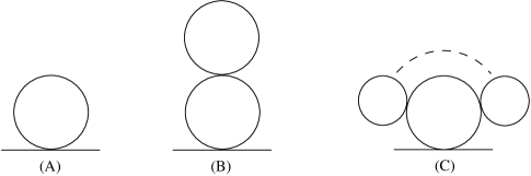
FIG. 1.: Bubble and cactus diagrams.

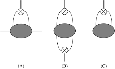
FIG. 2.: Diagrams which contain UV divergences as a result of the multiple insertion of $(1/2)\chi\phi^{2}$. (A) corresponds to a single insertion with two external lines. (B) and (C) have no external lines with a single insertion and a double insertion, respectively.

  

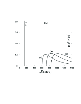
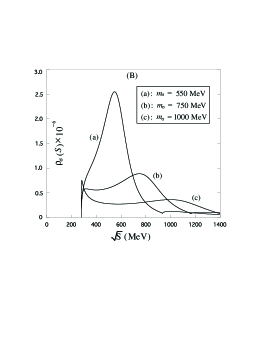
FIG. 3.: Spectral functions at $T=0$ in the $\pi$ channel (A) and in the $\sigma$ channel (B) for $m^{peak}_{\sigma}=550$ MeV, 750 MeV and 1000 MeV.

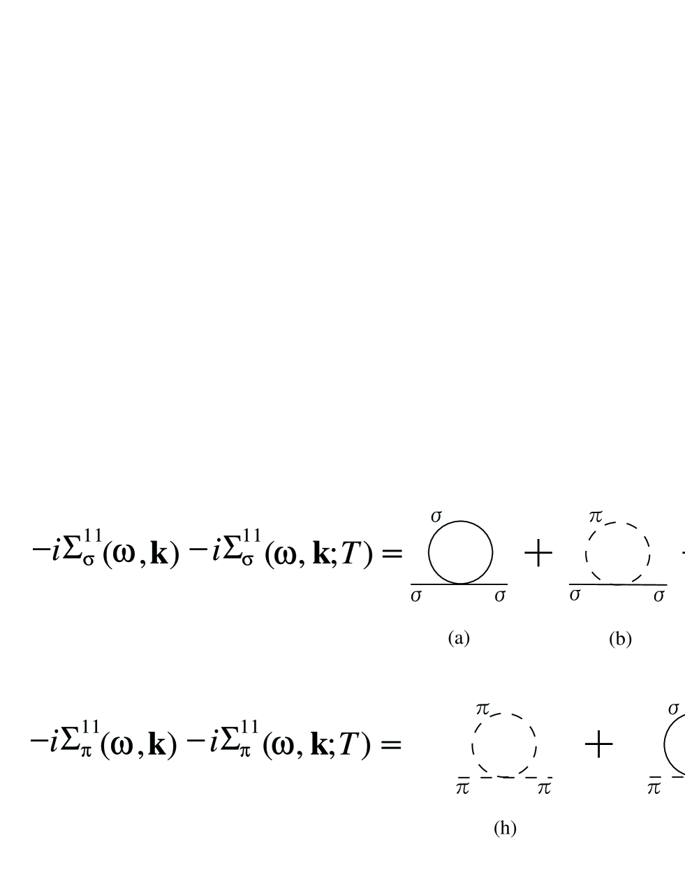
FIG. 4.: One-loop self-energy $\Sigma^{11}$ for $\sigma$ and $\pi$ in the modified loop-expansion at finite $T$.

  

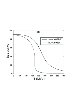
FIG. 5.: (A) Masses in the tree-level $m_{0\pi}(T)$ and $m_{0\sigma}(T)$ shown with left vertical scale, and the mass parameter $m^{2}(T)$ with the right vertical scale. (B) $\xi(T)$ for $m_{\pi}(T=0)=140$MeV and 30 MeV with $m^{peak}_{\sigma}(T=0)=550$ MeV.

  

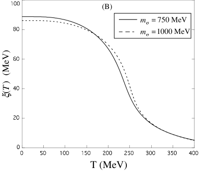
FIG. 6.: (A) Masses in the tree-level $m_{0\pi}(T)$ and $m_{0\sigma}(T)$. (B) $\xi(T)$ for $m^{peak}_{\sigma}(T=0)=750$MeV and 1000 MeV with $m_{\pi}=140$ MeV.

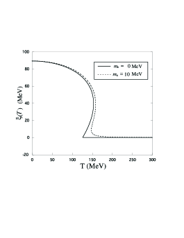
FIG. 7.: $\xi(T)$ for $m^{peak}_{\sigma}(T=0)=550$MeV with $m_{\pi}=0$ MeV and $m_{\pi}=10$ MeV.

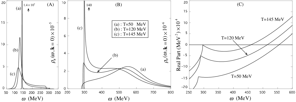
FIG. 8.: Spectral function in the $\pi$ channel (A) and in the $\sigma$ channel (B) for $T=50,120,145$ MeV with $m^{peak}_{\sigma}(T=0)=550$ MeV. The real part of $(D_{\sigma}^{R}(\omega,0;T))^{-1}$ as a function of $\omega$ is shown in (C).

  

FIG. 9.: (A) Spectral functions in the $\pi$ and $\sigma$ channels at $T=180$ MeV. (B) The real part of $(D_{\pi}^{R}(\omega,0;T))^{-1}$ and $(D_{\sigma}^{R}(\omega,0;T))^{-1}$ as a function of $\omega$ at $T=180$ MeV with $m^{peak}_{\sigma}(T=0)=550$ MeV.

FIG. 10.: Diphoton yield per unit space-time volume in the back to back kinematics at T=145 MeV for $m^{peak}_{\sigma}(T=0)=550$ MeV.

REFERENCES

- [1]
- [2] Quark Matter ’96, Nucl. Phys. A610 (1996). Quark Matter ’97, Nucl. Phys. A (1998) in press.
- [3] LATTICE ’96, Nucl. Phys. B (Proc. Suppl.) 53, (1997).
- [4] A. Ukawa, Nucl. Phys. B (Proc. Suppl.) 53, 106, (1997).
- [5] See examples quoted in Basic Notion of Condensed Matter Physics, P. W. Anderson, (Benjamin, California, 1984); Phasenübergänge and Kritische Phänomene, W. Gebhardt and U. Krey, (Friedr. Vieweg & Sohn, Wiesbaden, 1980).
- [6] T. Hatsuda and T. Kunihiro, Phys. Rep. 247, 221 (1994).
- [7] K. Rajagopal, in Quark-Gluon Plasma 2, ed. R. Hwa (World Scientific, Singapore, 1995).
- [8] S. Weinberg, Phys. Rev. D9, 3357 (1974). L. Dolan and R. Jackiw, Phys. Rev. D9, 3320 (1974).
- [9] D. A. Kirzhnits and A. D. Linde, Ann. Phys. 101, 195 (1976).
- [10] G. Baym and G. Grinstein, Phys. Rev. D15, 2897 (1977). H. E. Haber and H. A. Weldon, Phys. Rev. D25, 502 (1982). G. Amelino-Camelia and S-Y. Pi, Phys. Rev. D47, 2356 (1993). G. Amelino-Camelia, Nucl. Phys. B476, 255 (1996); Phys. Lett. B407, 268 (1997). H-S. Roh and T. Matsui, Eur. Phys. J. A1, 205 (1998). See also, H. Nakkagawa and H. Yokota, Mod. Phys. Lett. A11, 2259 (1996); Prog. Theor. Phys. Suppl. 129, 209 (1997). K. Ogure and J. Sato, hep-ph/9802418 (1998) and references therein.
- [11] S. Chiku and T. Hatsuda, Phys. Rev. D57, R6 (1998).
- [12] For applications of the mean-field method to field theories, see e.g. Y. Nambu and G. Jona-Lasinio, Phys. Rev. 122, 345 (1961). T. Kunihiro and T. Hatsuda, Prog. Theor. Phys. 71, 1332 (1984).
- [13] Since the number of works related to OPT is enormous, we quote only two books which contain the original references: G. A. Arteca, F. M. Fernández and E. A. Castro, Large Order Perturbation Theory and Summation Methods in Quantum Mechanics, (Springer-Verlag, Berlin, 1990). H. Kleinert, Path Integrals in Quantum Mechanics, Statistical and Polymer Physics, 2nd. edition (World Scientific, Singapore, 1995), Section 5. See also, T. Hatsuda, T. Kunihiro and T. Tanaka, Phys. Rev. Lett. 78, 3229 (1997); T. Tanaka, Phys. Lett. A238, 79 (1998).
- [14] A. Okopińska, Phys. Rev. D36, 2415 (1987); Mod. Phys. Lett. A12, 1003 (1997). (In the first reference, OPT at finite was examined with being a small perturbation, which is in contrast with our approach.) See also, G. A. Hajj and P. M. Stevenson, Phys. Rev. D37, 413 (1988).
- [15] N. Banerjee and S. Mallik, Phys. Rev. D43, 3368 (1991).
- [16] P.Fendley, Phys. Lett. B196, 175 (1987).
- [17] E. Braaten and R. D. Pisarski, Nucl. Phys. B337, 569 (1990); ibid. B339, 310 (1990). R. R. Parwani Phys. Rev. D45, 4695 (1992). P. Arnold and C-X. Zhai, Phys. Rev. D50, 7603 (1994); ibid. D51, 1906 (1995). See also, F. Karsch, A. Patkos and P. Petreczky, Phys. Lett. B401, 69 (1997).
- [18] See e.g., J. Negele and H. Orland, Quantum Many-Particle Systems, (Addison-Wesley, New York, 1988).
- [19] If we explicitly write in eq.(5), it appears as . Therefore, the loop-expansion by at finite does not coincide with the expansion. The expansion by should be regarded as a steepest descent evaluation of the functional integral [18].
- [20] R. E. Norton and J. M. Cornwall, Ann. Phys. 91, 106 (1975). M. B. Kislinger and P. D. Morley, Phys. Rev. D13, 2771 (1976). H. Matsumoto, I. Ojima and H. Umezawa, Ann. Phys. 152, 348 (1984). A. J. Niemi and G. W. Semenoff, Nucl. Phys. B230 [FS10], 181 (1984).
- [21] B. W. Lee, Nucl. Phys. B9, 649 (1969). B. W. Lee, Chiral Dynamics, (Gordon and Breach, New York, 1972).
- [22] T. Kugo, Prog Theor. Phys. 57, 593 (1977).
- [23] This point was first recognized in [15].
- [24] At finite or chemical potential, only the rotational symmetry in space is preserved in the rest frame of the heat-bath or matter. Therefore, in general.
- [25] S. Chiku and T. Hatsuda, under investigation.
- [26] P. M. Stevenson, Phys. Rev. D23, 2916 (1981).
- [27] Although at high coincides with the Debye screening mass for , they could be different in higher orders: Physical Debye mass is, in general, a function of .
- [28] In this case, at the stationary point of the thermal effective potential.
- [29] W. A. Bardeen and M. Mosche, Phys. Rev. D28, 1372 (1983).
- [30] See, e.g. C. Itzykson and J-B. Zuber, Quantum Field Theory, (McGraw-Hill, New York, 1985). T. Muta, Foundations of Quantum Chromodynamics, (World Scientific, Singapore, 1987).
- [31] See the following papers and the references quoted therein for the breakdown of the NG theorem in self-consistent methods and for attempts to cure the problem: A. Okopińska, Phys. Lett. B375, 213 (1996). A. Dmitrainović, J. A. McNeil and J. R. Shepard, Z. Phys. C69, 359 (1996). G. Amelino-Camelia, Phys. Lett. B407, 268 (1997).
- [32] T. Hatsuda and T. Kunihiro, Phys. Rev. Lett. 55, 158 (1985); Phys. Lett. B185, 304 (1987). Another interesting issue is the spectral change of vector mesons: R. D. Pisarski, Phys. Lett. B110, 155 (1982); G. E. Brown and M. Rho, Phys. Rev. Lett. 66, 2720 (1991); T. Hatsuda and S. H. Lee, Phys. Rev. C46 (1992) R34; T. Hatsuda, Y. Koike and S. H. Lee, Nucl. Phys. B394, 221 (1993).
- [33] H. A. Weldon, Phys. Lett. B274, 133 (1992). C. Song and V. Koch, Phys. Lett. B404, 1 (1997).
- [34] S. Huang and M. Lissia, Phys. Rev. D52, 1134 (1995); Phys. Lett. B348, 571 (1995); Phys. Rev. D53, 7270 (1996).
- [35] L. H. Chan and R. W. Haymaker, Phys. Rev. D7, 402 (1973); ibid. D10, 4170 (1974).
- [36] R. D. Pisarski and F. Wilczek, Phys. Rev. D29, 338 (1984). K. Rajagopal and F. Wilczek, Nucl. Phys. B399, 395 (1993). See also, M. Asakawa, Z. Huang and X.-N. Wang, Phys. Rev. Lett. 74, 3126 (1995); J. Randrup, Phys. Rev. D55, 1188 (1997) and references therein.
- [37] In the present paper, and the sign of are defined differently from those in [35]. Also in [35] should be considered as an unrenormalized parameter, while in the present paper is a renormalized one.
- [38] N. A. Törnqvist and M. Roos, Phys. Rev. Lett. 76, 1575 (1996). M. Harada, F. Sannino and J. Schechter, Phys. Rev. D54, 1991 (1996); Phys. Rev. Lett. 78, 1603 (1997). S. Ishida et al., Prog. Theor. Phys. 95, 745 (1996); ibid. 98, 1005 (1997). J. A. Oller, E. Oset and J. R. Peláez, Phys. Rev. Lett. 80, 3452 (1998). K. Igi and K. Hikasa, hep-ph/9807326 (1998).
- [39] B. Kastening, Phys. Lett. B283, 287 (1992). M. Bando, T. Kugo, N. Maekawa and H. Nakano, Phys. Lett. B301, 83 (1993); Prog. Theor. Phys. 90, 405 (1993).
- [40] M. Le Bellac, Thermal Field Theory, (Cambridge Univ. Press, Cambridge, 1996).
- [41] M. Gell-Mann, R. J. Oakes and B. Renner, Phys. Rev. 175, 2195 (1968).
- [42] D. A. Kirzhnits and A. D. Linde, Ann. Phys. 101, 195 (1976). G. Baym and G. Grinstein, Phys. Rev. D15, 2897 (1977). H-S. Roh and T. Matsui, Eur. Phys. J. A1, 205 (1998).
- [43] We have studied the free energy as a function of near the chiral limit and found that it has a discontinuity at certain temperature between and . This is another sign that the first-order nature is an artifact of the approximation. (Remember that, the free energy must be a continuous function of irrespective of the order of the phase transition: see e.g. N. Goldenfeld, Lectures on Phase Transitions and the Renormalization Group, (Addison-Wesley, New York, 1992).)
- [44] See, K. Kanaya and S. Kaya, Phys. Rev. D51, 2404 (1995) and references therein.
- [45] H. Itoyama and A. H. Mueller, Nucl. Phys. B218, 349 (1983). E. V. Shuryak, Phys. Lett. B207, 345 (1988). J. L. Goity and H. Leutwyler, Phys. Lett. B228, 517 (1989). H. Leutwyler and A. V. Smilga, Nucl. Phys. B342, 302 (1990). R. D. Pisarski and M. Tytgat, Phys. Rev. D54, 2989 (1996).
- [46] A preliminary version of this study has been reported in S. Chiku, Prog. Theor. Phys. Suppl. 129, 91 (1998).
- [47] C. Gale and J. I. Kapusta, Nucl. Phys. B 357, 65 (1991).
- [48] S. Hafjitheodoridis and B. Moussallam, Phys. Rev. D37, 1331 (1988).
- [49] S. P. Klevansky, Nucl. Phys. A575, 605 (1994)
- [50] P. Rehberg, Yu. I. Kalinovskii and D. Blaschke, Nucl. Phys. A622 (1997) 478. In this paper, the mode couplings are not taken into account.
- [51] A. D. Linde, Phys. Lett. 96B, 289 (1980). See also, T. Hatsuda, Phys. Rev. D56, 8111 (1997) and references therein.