Chapter 0 Models of Electroweak Symmetry Breaking

1 Introduction

Discovering the dynamics responsible for electroweak symmetry breaking is the outstanding question facing particle physics today, and the answer will be found in the next decade. In these lectures I discuss the range of models which have been proposed to explain electroweak symmetry breaking. I begin with an overview of Higgs models, with emphasis on the naturalness/hierarchy and triviality problems, and then consider general lessons which can be drawn about the symmetry breaking sector in arbitrary scalar models. Subsequently, I discuss the symmetry breaking sector in supersymmetric models and then consider models of dynamical electroweak symmetry breaking. I conclude with a brief review of the open questions.

2 The Standard Model Higgs Boson

1 The Standard Model Higgs Sector

In the standard [3, 4] one-doublet Higgs model, one introduces a fundamental scalar particle

$${\phi=\left(\matrix{\phi^{+}\cr\phi^{0}\cr}\right)}{}~{}~{}~{},$$ (1)

which transforms as a $2_{+{1\over 2}}$ under $SU(2)_{W}\times U(1)_{Y}$. In order to break the electroweak interactions to electromagnetism, one introduces the potential

$$V(\phi)=\lambda\left(\phi^{\dagger}\phi-{v^{2}\over 2}\right)^{2}{}~{}~{}~{},$$ (2)

which is minimized for nonzero $\langle\phi\rangle$, breaking the electroweak gauge symmetry appropriately.

The potential in eq. (2) is necessarily $SU(2)_{W}\times U(1)_{Y}$ invariant. In fact, the potential has an additional symmetry [5] as well. To see this, define ${\tilde{\phi}=i\sigma_{2}\phi^{*}}$ and consider the $2\times 2$ matrix

$${\Phi=\left({\tilde{\phi}}\ {\phi}\right)}\ \ \rightarrow\ \ \Phi^{\dagger}\Phi=\Phi\Phi^{\dagger}={({\phi^{\dagger}\phi})\,{\cal I}}~{}.$$ (3)

Because of the pseudo-reality of the doublet representation of $SU(2)$, under $SU(2)_{L}\times U(1)_{Y}$, $\Phi\rightarrow{L}\Phi{R^{\dagger}}$, where

$${L}=\exp\left({i{w^{a}(x)}\sigma^{a}\over 2}\right)\ \ \ \&\ \ \ {R}=\exp\left({i{b(x)}\sigma^{3}\over 2}\right)~{},$$ (4)

with $L\in SU(2)_{W}$, $R\in U(1)_{Y}$, and where the $\sigma^{a}$ are the Pauli matrices. Note that $R$ acts as a $\sigma^{3}$ rotation in an $SU(2)$ acting on $\Phi$ by multiplication on the right. In terms of this new field definition, the lagrangian for the Higgs sector can be written

$${1\over 2}{\rm Tr}\left(D^{\mu}\Phi D_{\mu}\Phi^{\dagger}\right)+{\lambda\over 4}\left({\rm Tr}\left(\Phi\Phi^{\dagger}\right)-v^{2}\right)^{2}~{},$$ (5)

with

$$D_{\mu}\Phi=\partial_{\mu}\Phi+{\rm i}g{\rm\bf W}_{\mu}\Phi-{\rm i}\Phi g^{\prime}{\rm\bf B}_{\mu}~{},$$ (6)

where ${\rm\bf W}_{\mu}=W^{a}_{\mu}\sigma^{a}/2$ and ${\rm\bf B}_{\mu}=B_{\mu}\sigma^{3}/2$. Note that the potential in eq. (5) has a manifest $SU(2)_{L}\times SU(2)_{R}$ global symmetry, larger than required by the $SU(2)_{W}\times U(1)_{Y}$ gauge symmetry.

The effect of symmetry breaking is easily seen using the “polar decomposition” of $\Phi$. By eq. (3) we see that $\Phi$ may be written as a real scalar field times a unitary matrix

$$\Phi(x)={1\over\sqrt{2}}\,({H(x)}+v)\,{\Sigma(x)}~{},$$ (7)

with

$${\Sigma(x)}=\exp(i{\pi^{a}(x)}\sigma^{a}/v)~{}.$$ (8)

In unitary gauge we may set $\langle\Sigma\rangle={\cal I}$. This symmetry breaking reduces the gauge symmetry to electromagnetism, and breaks the global $SU(2)_{L}\times SU(2)_{R}$ symmetry discussed above to a vectorial $SU(2)_{V}$ “custodial” [6] symmetry. For every linearly-independent spontaneously broken global symmetry, there must be a Goldstone boson. From the three broken symmetries above we obtain the $\pi^{\pm}$ and $\pi^{0}$ which, by the Higgs mechanism, become the longitudinal components, $W^{\pm}_{L}$ and $Z_{L}$, of the weak gauge bosons. The remaining degree of freedom, $H(x)$, is the Higgs field.

The mass of the $W$ can be calculated directly from the lagrangian in eq. (5) to be

$$M_{W}={gv\over 2}\rightarrow v\approx 246{\rm GeV}~{}.$$ (9)

The mass of the neutral gauge boson is somewhat more complicated since there is mixing between the neutral $SU(2)_{W}$ gauge boson and the $U(1)_{Y}$ gauge boson. A complete analysis requires computing the full mass-squared matrix of all four gauge bosons

$$M^{2}={v^{2}\over 2}\left(\matrix{g^{2}&&&\cr&g^{2}&&\cr&&g^{2}&-gg^{\prime}\cr&&-gg^{\prime}&{g^{\prime}}^{2}\cr}\right)~{},$$ (10)

which results in

$$\rho\equiv{M^{2}_{W}\over M^{2}_{Z}\cos^{2}\theta_{W}}=1~{}.$$ (11)

This prediction, one of the first in modern electroweak theory, insures the equality of the strength of deep-inelastic charged- and neutral-current interactions and, after properly accounting for small corrections discussed below, its validity has been verified to a fraction of a percent.

It is important to appreciate that the form of the electroweak gauge boson mass matrix and hence the relation eq. (11) is a consequence of the residual $SU(2)_{V}$ custodial symmetry. This symmetry requires that, in the limit $g^{\prime}\to 0$, the $SU(2)_{L}$ gauge bosons must be degenerate, since they form an irreducible representation of the custodial group. This, plus the constraint that $m_{\gamma}=0$, insures that the gauge boson mass matrix is proportional to the matrix shown above.

2 Violations of Custodial Symmetry

Custodial $SU(2)_{V}$ is a symmetry of the Higgs potential, but not of Higgs interactions. For example, the hypercharge interactions (cf. eq. (6)), and hence electromagnetism violate custodial symmetry. Therefore there are contributions to $\Delta\rho\equiv\rho-1$

(12)

of ${\cal O}(\alpha)$. Furthermore, the Higgs boson must couple to the ordinary fermions in order to give rise to their observed masses. Written in terms of $\Phi$, the Yukawa couplings of the scalar doublet to the third generation is

$$\left(\matrix{\bar{t}_{L}&\bar{b}_{L}\cr}\right)\Phi\left(\matrix{y_{t}&\cr&y_{b}\cr}\right)\left(\matrix{t_{R}\cr b_{R}}\right)~{},$$ (13)

and violates custodial $SU(2)_{V}$ since

$$y_{t}\equiv{{\sqrt{2}m_{t}}\over v}\gg y_{b}\equiv{{\sqrt{2}m_{b}}\over v}~{}.$$ (14)

Contributions to the gauge-boson self-energies from

      (15)

give rise to

$$\Delta\rho\approx{3y^{2}_{t}\over 32\pi^{2}}\approx 1\%\,\left({m_{t}\over 175{\rm GeV}}\right)^{2}\,.$$ (16)

It is also important to note that custodial $SU(2)_{V}$ is an accidental symmetry: it is a symmetry of all $SU(2)_{L}\times U(1)_{Y}$ invariant terms of dimension 4 or less in the Higgs sector of the lagrangian in the limit $g^{\prime}\to 0$. It can be violated by terms of higher dimension [7, 8] arising from physics at some higher scale, e.g.

$$(\phi^{\dagger}D^{\mu}\phi)(\phi^{\dagger}D_{\mu}\phi)={1\over 4}\left({\rm Tr}\,\sigma_{3}\Phi^{\dagger}D^{\mu}\Phi\right)\left({\rm Tr}\,\sigma_{3}\Phi^{\dagger}D_{\mu}\Phi\right)~{}.$$ (17)

3 The Higgs Boson

Figure 1: Higgs decay branching ratios as a function of Higgs mass. All decays proceed through the couplings in eq. (19), with the exception of the $\gamma\gamma$ mode which occurs through a fermion or gauge-boson loop. From ref. [9].

At tree-level, the Higgs Boson mass can be calculated directly from the potential

$$m^{2}_{H}=2\lambda v^{2}~{}.$$ (18)

As the masses of all of the standard model particles arise from the vacuum expectation value of $\phi$, the tree-level couplings of the Higgs are also immediately determined to be

$${\cal L}\supset\left(1+{H\over v}\right)^{2} \left[M^{2}_{W}W^{\mu+}W_{\mu}^{-}+{1\over 2}M^{2}_{Z}Z^{\mu}Z_{\mu}\right]$$ (19)

$$-\left(1+{H\over v}\right)\left[\sum_{i}m_{i}\bar{\psi_{i}}\psi_{i}\right]~{}.$$

As a function of the Higgs boson mass, we then find the branching ratios shown in fig. 1.

The best direct experimental limits on the Higgs boson come from the non-observation of the process $e^{+}e^{-}\to Z^{*}\to ZH$ at LEPII. Recent results, shown in fig. 2, give a lower bound of 82 GeV on the Higgs boson mass at 95% confidence level. Future observations at the LEPII and the Tevatron could discover a Higgs boson up to a mass of order 120-130 GeV [10, 11].

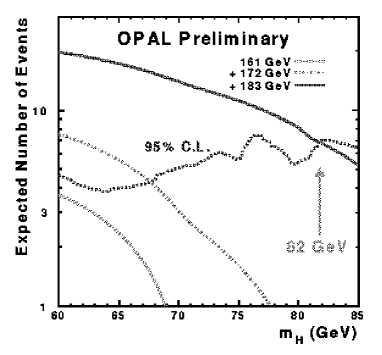
Figure 2: OPAL limits on the standard model Higgs boson. As shown, the preliminary bound from the run at 183 GeV imply that $m_{H}>82$ GeV at 95% confidence level. From ref. [12].

Precision measurements of electroweak quantities at LEP, SLC, and in low-energy experiments can also, in principle, constrain the allowed values of $m_{H}$. At one-loop, the relationship between $G_{F}$, $\alpha_{em}$, $M_{Z}$ and any electroweak observable depends on the Higgs mass and the top-quark mass. The collection of precision measurements can then give an “allowed” region of top-quark and Higgs masses. This allowed region can be illustrated in the $(m_{t},M_{W})$ plane, as shown in fig. 3. The solid curve gives the bounds at 68% confidence level coming from precision electroweak tests, the dashed curve gives the 68% bounds on $m_{t}$ coming from measurements at CDF and DØ, and on $M_{W}$ coming from measurements at these experiments and experiments at LEPII. The shaded band shows the predictions of the standard model for Higgs masses between 60 and 1000 GeV.

Figure 3: The allowed region in the $(m_{t},M_{W})$ plane coming from precision electroweak tests at 68% confidence level (solid curve) and from direct measurement (dashed curve). Also shown is the standard model prediction of $M_{W}$ as a function of $m_{t}$ for various Higgs boson masses from 60 GeV to 1000 GeV. From ref. [13]

The consistency of the standard model prediction and the indirect and direct measurements of $m_{t}$ and $M_{W}$ is a remarkable triumph of the standard model. Nonetheless, at 95% or 99% confidence level, these measurements do not currently provide a significant constraint on the Higgs boson mass.

The raison d’être of the LHC is to uncover the agent of electroweak symmetry breaking. The experimental prospects for discovery of a Higgs boson in the “gold-plated” $H\to ZZ\to 4\ell$ mode is shown in fig. 4.

Figure 4: Significance of Higgs boson discovery signal in the channel $H\to ZZ\to 4\ell$ for various integrated luminosities (n.b. $10^{5}$ pb^-1 equals one year at design luminosity). From ref. [14].

When other modes, in particular $H\to ZZ\to 2\ell 2\nu$ and $H\to WW\to\ell\nu jj$ for a heavy Higgs boson and $H\to\gamma\gamma$ for a light Higgs boson, are considered, the LHC should be able to discover a Higgs boson with a mass ranging from the ultimate LEP II/Tevatron limit ($\sim$ 100 – 130 GeV) to 800 GeV [11].

We can obtain a theoretical upper bound on the Higgs boson mass from unitarity [15, 16]. Consider (formally) the limit $\lambda\to\infty$. The Higgs degree of freedom becomes heavy and may formally be “integrated out” of the theory:

$$\Phi(x)={1\over\sqrt{2}}\,({H(x)}+v)\,{\Sigma(x)}\to{v\over\sqrt{2}}{\Sigma(x)}~{}.$$ (20)

In this limit, the Higgs sector is equivalent to an effective chiral theory for the symmetry breaking pattern $SU(2)_{L}\times SU(2)_{R}$ $\to$ $SU(2)_{V}$. Allowing for custodial $SU(2)$ violation, the most general such effective lagrangian [17, 18] at ${\cal O}(p^{2})$ may be written:

$${{v^{2}\over 4}{\rm Tr}\left[D^{\mu}\Sigma^{\dagger}D_{\mu}\Sigma\right]+{v^{2}\over 4}({1\over\rho}-1)\left[{\rm Tr}\sigma_{3}\Sigma^{\dagger}D^{\mu}\Sigma\right]^{2}}~{}.$$ (21)

Setting $\Sigma=1$ in unitary gauge, we find

$${g^{2}v^{2}\over 4}W_{-}^{\mu}W_{\mu+}+{g^{2}v^{2}\over{8\rho\cos^{2}\theta}}Z^{\mu}Z_{\mu}~{}~{}~{},$$ (22)

as required.

Now consider what happens when these massive $W$ and $Z$ bosons scatter. At high-energies we can use the equivalence theorem [19, 20, 21]

$${\cal A}(W_{L}W_{L})={\cal A}(\pi\pi)+{\cal O}({M_{W}\over E})\,.$$ (23)

to reduce the problem of longitudinal gauge boson ($W_{L}$) scattering to the corresponding problem of the scattering of the Goldstone bosons which would be present in the absence of the weak gauge interactions. At ${\cal O}(p^{2})$ results in [17, 18] universal low-energy theorems:

$${\cal M}[W^{+}_{L}W^{-}_{L}\to W^{+}_{L}W^{-}_{L}]= {{\textstyle iu}\over{\textstyle{v^{2}\rho}}}$$

$${\cal M}[W^{+}_{L}W^{-}_{L}\to Z_{L}Z_{L}]= {{\textstyle is}\over{\textstyle v^{2}}}\left(4-{{\textstyle 3}\over{\textstyle\rho}}\right)$$

$${\cal M}[Z_{L}Z_{L}\to Z_{L}Z_{L}]= 0~{}~{}~{}.$$ (24)

Note that these amplitudes grow as the square of the center-of-mass collision energy. Projecting onto the $I=J=0$ channel for $\rho=1$, we find

$${\cal A}_{00}={s\over 16\pi v^{2}}\approx\left({\sqrt{s}\over 1.8\,{\rm TeV}}\right)^{2}~{}.$$ (25)

Thus, in the absence of additional contributions, the isosinglet scalar scattering amplitude would violate unitarity at an energy scale of approximately 1.8 TeV. In the standard Higgs model, Higgs exchange unitarizes the cross section. From this we conclude [15, 16] that $m_{H}\begin{array}[]{c}<\vspace{-.7em}\\ {\scriptstyle\sim}\end{array}1.8$ TeV.

We can also obtain a theoretical lower bound on the Higgs mass from vacuum stability [22, 23, 24]. To investigate this effect, we must compute the “effective potential” [25], the sum of all one-particle irreducible diagrams in the presence of a constant external field background:

$$V(\phi)=V_{0}(\phi)+V_{1}(\phi)+\ldots$$ (26)

with, for example,

$$V_{1}(\phi)=\lower 4.0pt\hbox{{\epsfbox{figures/epot1.eps}}}+\lower 12.0pt\hbox{{\epsfbox{figures/epot2.eps}}}+\ldots$$ (27)

In the leading-log approximation the effective potential at large field-values may be written [25, 26]

$$V^{eff}(\phi,M)\approx\tilde{\lambda}(t)(\phi^{\dagger}\phi)^{2}\exp{\left(4\int_{0}^{t}dw{\gamma(w)\over{1-\gamma(w)}}\right)}$$ (28)

where $t=\log(\phi/M)$, $\gamma$ is the anomalous dimension of $\phi$, and

$${d\tilde{\lambda}\over dt}={\beta_{\lambda}\over{1-\gamma}}~{}.$$ (29)

This equation allows for a nice geometrical description of the Coleman-Weinberg mechanism [26].

At one loop, neglecting terms involving $\lambda$ (since we are investigating the possibility of a light Higgs boson) and light fermions

$$\beta_{\lambda}\approx{3\over 128\pi^{2}}\left[3g^{4}+2g^{2}{g^{\prime}}^{2}+{g^{\prime}}^{4}{-16y^{4}_{t}}\right]~{}.$$ (30)

Because of the large top-quark mass (with Yukawa coupling $y_{t}$), for small $m_{H}$ (and hence small $\lambda$) the perturbative vacuum is unstable at large $\phi$. This instability is illustrated in fig. 5.

Figure 5: Effective potential in leading-log approximation for $m_{H}=121.7$ GeV. From ref. [27].

If we require stability up to a scale $\Lambda$, where new-physics enters and additional terms $\propto(\phi^{\dagger}\phi)^{n}/\Lambda^{2n-4}$ can enter to stabilize the potential, we find a lower bound on $m_{H}$ as a function of this new energy scale. This bound is shown in in the lower curve in figure 6.

Figure 6: The lower curve graphs the lower bound on the Higgs mass as a function of energy scale $\Lambda$ obtained by requiring that the potential be stable out to field values of order $\Lambda$. The upper curve graphs the upper bound on the Higgs mass as a function of energy scale $\Lambda$ obtained by requiring that the Landau pole associated with the self-coupling $\lambda$ occur at a scale greater than $\Lambda$. From ref. [27].

3 Triviality and its Implications

While the standard model is simple and renormalizable, it has a number of shortcomings. First, while the theory can be constructed to accommodate the breaking of electroweak symmetry, it provides no explanation for it. One simply assumes that the potential is of the form in eq. (2). In addition, in the absence of supersymmetry, quantum corrections to the Higgs mass are naturally of order the largest scale in the theory

$${\lower 5.0pt\hbox{\epsfbox{figures/msq.eps}}}\ \rightarrow\ m_{H}^{2}\propto\Lambda^{2}~{},$$ (31)

leading to the hierarchy and naturalness problems [28]. Finally, the $\beta$ function for the self-coupling $\lambda$ is positive

$${\lower 7.0pt\hbox{\epsfbox{figures/beta.eps}}}\ \rightarrow\ \beta={3\lambda^{2}\over 2\pi^{2}}\,>\,0{}~{},$$ (32)

leading to a “Landau pole” and triviality [29, 30].

1 The Wilson Renormalization Group and Naturalness

The hierarchy,naturalness, and triviality problems can be nicely summarized in terms of the Wilson renormalization group [31, 29]. Define the theory with a fixed UV-cutoff:

$${\cal L}_{\Lambda}= D^{\mu}\phi^{\dagger}D_{\mu}\phi+m^{2}(\Lambda)\phi^{\dagger}\phi+{\lambda(\Lambda)\over 4}(\phi^{\dagger}\phi)^{2}$$ (33)

$$+{\hat{\kappa}(\Lambda)\over 36\Lambda^{2}}(\phi^{\dagger}\phi)^{3}+\ldots$$

Here $\hat{\kappa}$ is the coefficient of a representative irrelevant operator, of dimension greater than four. Next, integrate out states with $\Lambda^{\prime}<k<\Lambda$, and construct a new lagrangian with the same low-energy Green’s functions:

$${\cal L}_{\Lambda} \rightarrow {\cal L}_{\Lambda^{\prime}}$$

$$m^{2}(\Lambda) \rightarrow m^{2}(\Lambda^{\prime})$$

$$\lambda(\Lambda) \rightarrow \lambda(\Lambda^{\prime})$$

$$\hat{\kappa}(\Lambda) \rightarrow \hat{\kappa}(\Lambda^{\prime})$$ (34)

The low-energy behavior of the theory is then nicely summarized in terms of the evolution of couplings in the infrared. A three-dimensional representation of this flow in the infinite-dimensional space of couplings is shown in Figure 7.

Figure 7: Renormalization group flow of Higgs mass $m^{2}$, Higgs self-coupling $\lambda$, and the coefficient of a representative irrelevant operator $\hat{\kappa}$. The flows go from upper-left to lower-right as one scales to the infrared.

From Figure 7, we see that as we scale to the infrared the coefficients of irrelevant operators, such as $\hat{\kappa}$, tend to zero; i.e. the flows are attracted to the finite dimensional subspace spanned (in perturbation theory) by operators of dimension four or less; this is the modern understanding of renormalizability.

On the other hand, the coefficient of the only relevant operator (of dimension 2), $m^{2}$, tends to infinity. In the absence of a symmetry that protects the scalar mass (such as supersymmetry, see section 6 below), it is natural for the mass to be proportional to the largest scale present in the theory [28]. This is the naturalness problem: since we want $m^{2}\propto v^{2}$ at low energies we must adjust the value of $m^{2}(\Lambda)$ to a precision of

$${\Delta m^{2}(\Lambda)\over m^{2}(\Lambda)}\propto{v^{2}\over\Lambda^{2}}~{}.$$ (35)

We are sure that a large hierarchy of scales does exist between the electroweak scale and the grand-unified or Planck scales. We expect that, even in the presence of an extra symmetry which stabilizes the Higgs mass, there should be some dynamical explanation for the this large hierarchy. The construction of a model which does not suffer from the naturalness and hierarchy problems will motivate the discussion presented in sections 6 through 12.

2 Implications of Triviality

Central to our discussion here is the fact that the coefficient of the only marginal operator, $\lambda$, tends to zero because of the positive $\beta$ function. If we try to take the continuum limit, $\Lambda\to+\infty$, the theory becomes free (or trivial) [29, 30], and could not result in the observed symmetry breaking.

The triviality of the scalar sector of the standard one-doublet Higgs model implies that this theory is only an effective low-energy theory valid below some cut-off scale $\Lambda$. Physically this scale marks the appearance of new strongly-interacting symmetry-breaking dynamics. Examples of such high-energy theories include “top-mode” standard models [32, 33, 34, 35, 36, 37, 38], which we discuss in section 12, and composite Higgs models [39, 40, 41]. As the Higgs mass increases, the upper bound on the scale $\Lambda$ decreases. An estimate of this effect can be obtained by integrating the one-loop $\beta$-function, which yields

$$\lambda(m_{H})\stackrel{{\scriptstyle<}}{{\sim}}{{2\pi^{2}}\over 3\log{\Lambda\over m_{H}}}\,.$$ (36)

Using the relation $m^{2}_{H}=2\lambda(m_{H})v^{2}$ we find

$$m^{2}_{H}\ln\left({\Lambda\over m_{H}}\right)\leq{4\pi^{2}v^{2}\over 3}~{}.$$ (37)

Hence a lower bound [42, 43] on $\Lambda$ yields an upper bound on $m_{H}$. We must require that $m_{H}/\Lambda$ in eq. (37) be small enough to afford the effective Higgs theory some range of validity (or to minimize the effects of regularization in the context of a calculation in the scalar theory).

Non-perturbative [44, 45, 46, 47, 48, 49] studies on the lattice using analytic and Monte Carlo techniques result in an upper bound on the Higgs mass of approximately 700 GeV. The lattice Higgs mass bound is potentially ambiguous because the precise value of the bound on the Higgs boson’s mass depends on the (arbitrary) restriction placed on $M_{H}/\Lambda$. The “cut-off” effects arising from the regulator are not universal: different schemes can give rise to different effects of varying sizes and can change the resulting Higgs mass bound.

On the other hand, we show below that, for models that reproduce the standard one-doublet Higgs model at low energies, electroweak and flavor phenomenology provide a lower bound on the scale $\Lambda$ of order 10 – 20 TeV. This limit is regularization-independent (i.e. independent of the details of the underlying physics). Using eq. (37) we estimate that this gives an upper bound of 450 – 500 GeV on the Higgs boson mass. The discussion we will present is based on perturbation theory and is valid in the domain of attraction of the “Gaussian fixed point” ($\lambda=0$). In principle, however, the Wilson approach can be used non-perturbatively, even in the presence of nontrivial fixed points or large anomalous dimensions. In a conventional Higgs theory, neither of these effects is thought to occur [44, 45, 46, 47, 48, 49].

3 Dimensional Analysis

We will analyze the effects of the underlying physics by estimating the sizes of various operators in a low-energy effective lagrangian containing the (presumably composite) Higgs boson and the ordinary gauge bosons and fermions. Since we are considering theories with a heavy Higgs field, we expect that the underlying high-energy theory will be strongly interacting. Borrowing a technique from QCD we will rely on dimensional analysis [50, 51] to estimate the sizes of various effects of the underlying physics.

A strongly interacting theory has no small parameters. As noted by Georgi [52], a theory with light scalar particles belonging to a single symmetry-group representation depends on two parameters: $\Lambda$, the scale of the underlying physics, and $f$ (the analog of $f_{\pi}$ in QCD), which measures the amplitude for producing the scalar particles from the vacuum. Our estimates will depend on the ratio $\kappa=\Lambda/f$, which is expected to fall between 1 and $4\pi$.

Consider the kinetic energy of a scalar bound-state in the appropriate low-energy effective lagrangian. The properly normalized kinetic energy is

$$\partial^{\mu}\phi^{\dagger}\partial_{\mu}\phi={\Lambda^{2}f^{2}}\left({\partial^{\mu}\over{\Lambda}}\right)\left({\phi^{\dagger}\over{f}}\right)\left({\partial_{\mu}\over{\Lambda}}\right)\left({\phi\over{f}}\right)~{}.$$ (38)

Here, because the fundamental scale of the interactions is $\Lambda$, we ascribe a $\Lambda$ to each derivative, and we associate an $f$ with each $\phi$ since $f$ measures the amplitude to produce the bound state. This tells us that the overall magnitude of each term in the effective lagrangian is ${\cal{O}}(f^{2}\Lambda^{2})$. We can next estimate the “generic” size of a mass term in the effective theory:

$$m^{2}\phi^{\dagger}\phi={\Lambda^{2}f^{2}}\left({\phi^{\dagger}\over{f}}\right)\left({\phi\over{f}}\right)\ \rightarrow\ {m^{2}\propto\Lambda^{2}}~{}.$$ (39)

This is the hierarchy problem in a nutshell. In the absence of some other symmetry not accounted for in these rules, fine-tuning is required to obtain $m^{2}\ll\Lambda^{2}$. Next, consider the size of scalar interactions. From the simplest interaction

$$\lambda(\phi^{\dagger}\phi)^{2}\ \rightarrow\ {\lambda\propto\left({\Lambda\over f}\right)^{2}=\kappa^{2}}~{},$$ (40)

we see that $\kappa$ will determine the size of coupling constants. Similarly, for a higher-dimension interaction such as the one in eq. (33) we find

$${\hat{\kappa}\over{\Lambda^{2}}}(\phi^{\dagger}\phi)^{3}\ \rightarrow\ {\hat{\kappa}\propto\kappa^{4}}~{}.$$ (41)

These rules are easily extended to include strongly-interacting fermions self-consistently. Again, we start with the properly normalized kinetic-energy

$$\bar{\psi}\hbox to0.0pt{\hbox to5.30904pt{\hfil/\hfil}\hss}\partial\psi={\Lambda^{2}f^{2}}\left({\bar{\psi}\over{f\sqrt{\Lambda}}}\right)\left({\hbox to0.0pt{\hbox to5.30904pt{\hfil/\hfil}\hss}\partial\over{\Lambda}}\right)\left({\psi\over{f\sqrt{\Lambda}}}\right)~{},$$ (42)

and learn that $f\sqrt{\Lambda}$ is a measure of the amplitude for producing a fermion from the vacuum. Next, consider a Yukawa coupling of a strongly-interacting fermion to our composite Higgs,

$$y(\bar{\psi}\phi\psi)\ \rightarrow\ {y\propto\kappa}~{}.$$ (43)

And finally, the natural size of a four-fermion operator is

$${\nu\over{\Lambda^{2}}}(\bar{\psi}\psi)^{2}\ \rightarrow\ {\nu\propto\kappa^{2}}~{}.$$ (44)

We will rely on these estimates to derive bounds on the scale $\Lambda$. By way of justification, we note that these estimates work in QCD for the chiral lagrangian [50, 51], with $f\to f_{\pi}$, $\Lambda\to 1$ GeV, and $\kappa\approx{\cal{O}}(4\pi)$. For example, four-nucleon operators of the form shown in eq. (44) arise in the vector channel from $\rho$-exchange and we obtain $\Lambda=m_{\rho}$ and $\kappa=g_{\rho}\approx 6$. In a QCD-like theory with $N_{c}$ colors and $N_{f}$ flavors one expects [53] that

$$\kappa\approx\min\left({4\pi a\over N_{c}^{1/2}},{4\pi b\over N_{f}^{1/2}}\right)~{},$$ (45)

where $a$ and $b$ are constants of order 1. In the results that follow, we will display the dependence on $\kappa$ explicitly; when giving numerical examples, we set $\kappa$ equal to the geometric mean of 1 and $4\pi$, i.e. $\kappa\approx 3.5$.

4 Isospin Violation and Bounds on $m_{H}$

Because of the $SU(2)_{W}\times U(1)_{Y}$ symmetry of the low-energy theory, all terms of dimension less than or equal to four respect custodial symmetry [5, 6]. The leading custodial-symmetry violating operator is of dimension six [7, 8] and involves four Higgs doublet fields $\phi$. According to the rules of dimensional analysis, the operator

$${\lower 35.0pt\hbox{\epsfbox{figures/fourhiggs.eps}}}\rightarrow{\kappa^{2}\over\Lambda^{2}}(\phi^{\dagger}D^{\mu}\phi)(\phi^{\dagger}D_{\mu}\phi)~{},$$ (46)

should appear in the low-energy effective theory with a coefficient of order one [8]. Such an operator will give rise to a deviation

$$\Delta\rho_{*}=-{\cal O}\left(\kappa^{2}{v^{2}\over\Lambda^{2}}\right)~{},$$ (47)

where $v\approx 246$ GeV is the expectation value of the Higgs field. Imposing the constraint [54, 55] that $|\Delta\rho_{*}|\leq 0.4\%$, we find the lower bound

$$\Lambda\stackrel{{\scriptstyle>}}{{\sim}}4\,{\rm TeV}\cdot\kappa~{}.$$ (48)

For $\kappa\approx 3.5$, we find $\Lambda\stackrel{{\scriptstyle>}}{{\sim}}14$ TeV.

Alternatively, it is possible that the underlying strongly-interacting dynamics respects custodial symmetry. Even in this case, however, there must be custodial-isospin-violating physics (analogous to extended-technicolor [56, 57] interactions) which couples the $\psi_{L}=(t,\ b)_{L}$ doublet and $t_{R}$ to the strongly-interacting “preon” constituents of the Higgs doublet in order to produce a top quark Yukawa coupling at low energies and generate the top quark mass. If, for simplicity, we assume that these new weakly-coupled custodial-isospin-violating interactions are gauge interactions with coupling $g$ and mass $M$, dimensional analysis allows us to estimate the size of the resulting top quark Yukawa coupling. The “natural size” of a Yukawa coupling (eq. (43)) is $\kappa$ and that of a four-fermion operator (eq. (44)) is $\kappa^{2}/\Lambda^{2}$; the ratio $(g^{2}/M^{2})/(\kappa^{2}/\Lambda^{2})$ is the “small parameter” associated with the extra flavor interactions and we find

$${\lower 35.0pt\hbox{\epsfbox{figures/yukawa.eps}}}\rightarrow{g^{2}\over M^{2}}{\Lambda^{2}\over\kappa}\bar{q}_{R}\phi\psi_{L}~{}.$$ (49)

In order to give rise to a quark mass $m_{q}$, the Yukawa coupling must be equal to

$${\sqrt{2}m_{q}\over v}$$ (50)

where $v\approx 246$ GeV. This implies

$$\Lambda\stackrel{{\scriptstyle>}}{{\sim}}{M\over g}\sqrt{\sqrt{2}\kappa{m_{q}\over v}}~{}.$$ (51)

These new gauge interactions will typically also give rise to custodial-isospin-violating 4-preon interactions which, at low energies, will give rise to an operator of the same form as the one in eq. (46). Using dimensional analysis, we find

$${\lower 35.0pt\hbox{\epsfbox{figures/yukawaiso.eps}}}\rightarrow\left[{{g^{2}\over M^{2}}}\left({{\kappa^{2}\over\Lambda^{2}}}\right)^{-1}\right]{\kappa^{2}\over\Lambda^{2}}(\phi^{\dagger}D^{\mu}\phi)(\phi^{\dagger}D_{\mu}\phi)~{},$$ (52)

which results in the bound $M/g\stackrel{{\scriptstyle>}}{{\sim}}4$ TeV. From eq. (51) with $m_{t}\approx 175$ GeV we then derive the limit

$$\Lambda\stackrel{{\scriptstyle>}}{{\sim}}4\,{\rm TeV}\cdot\sqrt{\kappa}~{}.$$ (53)

For $\kappa\approx 3.5$, we find $\Lambda\stackrel{{\scriptstyle>}}{{\sim}}7.5$ TeV.

As previously discussed, a lower bound on the scale $\Lambda$ yields an upper bound on the Higgs boson mass. Here we provide an estimate of this upper bound by naive extrapolation of the lowest-order perturbative result shown in eq. (37). For $\Lambda\stackrel{{\scriptstyle>}}{{\sim}}7.5$ TeV, this results in the bound $m_{H}\stackrel{{\scriptstyle<}}{{\sim}}550$ GeV.

4 Two-Higgs Doublet Model

1 The Higgs Potential and Boson Masses

Up to this point, we have discussed the simplest model which can account for electroweak symmetry breaking, the one-doublet Higgs model. In this case, the electroweak breaking sector consists of only one field. In general, the symmetry breaking sector can be more complicated. As a case study of an extended symmetry breaking sector, we next consider a model with two Higgs fields

$$\phi_{1}=\left(\matrix{\phi_{1}^{+}\cr\phi_{1}^{0}\cr}\right)\ \ \ \&\ \ \ \phi_{2}=\left(\matrix{\phi_{2}^{+}\cr\phi_{2}^{0}\cr}\right){}~{}~{}~{}.$$ (54)

The most general potential for such a model, with a softly broken $\phi_{1}\to-\phi_{1}$ symmetry (the necessity of which will be discussed in the following), is

$$\hskip-5.0ptV(\phi_{1},\phi_{2}) = \lambda_{1}(\phi^{\dagger}_{1}\phi_{1}-{v_{1}^{2}}/2)^{2}+\lambda_{2}(\phi^{\dagger}_{2}\phi_{2}-{v_{2}^{2}}/2)^{2}$$ (55)

$$+ \lambda_{3}\left[(\phi^{\dagger}_{1}\phi_{1}-{v_{1}^{2}}/2)+(\phi^{\dagger}_{2}\phi_{2}-{v_{2}^{2}}/2)\right]^{2}$$

$$+ {\lambda_{4}}\left[(\phi^{\dagger}_{1}\phi_{1})(\phi^{\dagger}_{2}\phi_{2})-(\phi^{\dagger}_{1}\phi_{2})(\phi^{\dagger}_{2}\phi_{1})\right]$$

$$+ {\lambda_{5}}\left[{\rm Re}(\phi^{\dagger}_{1}\phi_{2})-{v_{1}}{v_{2}}\cos\xi/2\right]^{2}$$

$$+ {\lambda_{6}}\left[{\rm Im}(\phi^{\dagger}_{1}\phi_{2})-{v_{1}}{v_{2}}\sin\xi/2\right]^{2}~{}.$$

For a range of $\lambda_{i}$ and for $v^{2}_{1},\,v^{2}_{2}>0$, the potential is minimized when

$$\langle\phi_{1}\rangle=\left(\begin{array}[]{c}0\\ {{v_{1}}/\sqrt{2}}\end{array}\right)\ \ \ \&\ \ \ \langle\phi_{2}\rangle=\left(\begin{array}[]{c}0\\ {{v_{2}}e^{i\xi}/\sqrt{2}}\end{array}\right)~{}.$$ (56)

In this vacuum, $SU(2)_{W}\times U(1)_{Y}\to U(1)_{em}$ with

$$M^{2}_{W}={g^{2}\over 2}({v^{2}_{1}}+{v^{2}_{2}})\ \ \ \&\ \ \ \rho={M_{W}\over M_{Z}\cos\theta_{W}}\equiv 1~{}.$$ (57)

From this we conclude that

$$v^{2}_{1}+v^{2}_{2}=v^{2}\approx(246\,{\rm GeV})^{2}.$$ (58)

Figure 8: Viewed as a system of coupled pendula, the Goldstone bosons correspond to the symmetric mode at left, and the pseudo-Goldstone bosons to the asymmetric mode at right.

Two complex Higgs doublets correspond to eight real degrees of freedom. The eight mass eigenstates can readily be determined from the potential. In what follows, we will make the simplifying assumption that $\sin\xi=0$, which avoids CP-violation in the symmetry breaking sector. One may view the mass eigenstates as normal modes of a system of coupled pendula (see Fig. 8). Defining ${\cos\beta=v_{1}/v}$ and ${\sin\beta=v_{2}/v}$, we find that the three “eaten” Goldstone bosons (which become the longitudinal components of the $W$ and $Z$) may be viewed as the “symmetric oscillation mode”:

$$G^{{\pm},0}=(\phi^{\pm}_{1},\sqrt{2}\,{\rm Im}\,\phi^{0}_{1}){\cos\beta}+(\phi^{\pm}_{2},\sqrt{2}\,{\rm Im}\,\phi^{0}_{2}){\sin\beta}~{}.$$ (59)

The three fields orthogonal to the Goldstone modes are physical pseudo-scalars

$$(H^{\pm},A^{0})=-(\phi^{\pm}_{1},\sqrt{2}\,{\rm Im}\phi^{0}_{1}){\sin\beta}+(\phi^{\pm}_{2},\sqrt{2}\,{\rm Im}\phi^{0}_{2}){\cos\beta}~{},$$ (60)

and have masses

$$m^{2}_{H^{\pm}}={\lambda_{4}}(v_{1}^{2}+v_{2}^{2})/2~{}~{}~{}{\neq}~{}~{}~{}m^{2}_{A^{0}}={\lambda_{6}}(v_{1}^{2}+v_{2}^{2})/2~{}.$$ (61)

In addition to the oscillation modes, there are two “breathing” modes in which the lengths of the pendula (Higgs doublet fields) change. These modes correspond to two neutral scalar fields. Defining

$$(H_{1},H_{2})=(\sqrt{2}\,{\rm Re}\,\phi^{0}_{1,2}-v_{1,2})~{},$$ (62)

we find the $2\times 2$ mass matrix

$$\left(\begin{array}[]{cc}2v_{1}^{2}(\lambda_{1}+\lambda_{3})+v_{2}^{2}\lambda_{5}/2&(4\lambda_{3}+\lambda_{5})v_{1}v_{2}/2\\ (4\lambda_{3}+\lambda_{5})v_{1}v_{2}/2&2v_{1}^{2}(\lambda_{2}+\lambda_{3})+v_{2}^{2}\lambda_{5}/2\end{array}\right)$$ (63)

The mass eigenstates define a mixing-angle $\alpha$

$$H^{0} = H_{1}\cos\alpha+H_{2}\sin\alpha$$

$$h^{0} = -H_{1}\sin\alpha+H_{2}\cos\alpha~{}.$$ (64)

2 Neutral Scalars

As in the case of the one-doublet model, the high-energy scattering of longitudinally-polarized electroweak gauge bosons is unitarized by the exchange of neutral scalars. The coupling of the neutral scalars to the $W$’s can be written

$${\cal L} \supset \left(1+2{{H_{1}}\over v}{\cos\beta}+2{{H_{2}}\over v}{\sin\beta}\right)$$ (65)

$$\ \times\ \left[M^{2}_{W}W^{\mu+}W_{\mu}^{-}+{1\over 2}M^{2}_{Z}Z^{\mu}Z_{\mu}\right]~{}.$$

changing basis from $(H_{1},H_{2})$ to $(h^{0},H^{0})$ amounts to replacing $\beta$ in eq. (65) with $(\beta-\alpha)$. Note that the exchange of both $h^{0}$ and $H^{0}$ is required to maintain unitarity, and from eq. (25) we conclude that $m_{h^{0},H^{0}}\begin{array}[]{c}<\vspace{-.7em}\\ {\scriptstyle\sim}\end{array}1.8$ TeV.

In the one-doublet model, the couplings of the single Higgs boson to the fermions were proportional to the fermion masses, eq. (19). For this reason, the couplings were manifestly flavor-diagonal. In the most general two-Higgs model, it is possible for each fermion species to acquire mass from the vacuum expectation value of both Higgs fields. In this case, it is not possible to ensure that the couplings of the $h^{0}$ and $H^{0}$ are flavor-diagonal, i.e. Higgs exchange could give rise to flavor-changing neutral-currents.

In order to avoid this possibility, it is necessary to ensure that each species of fermion couples to one and only one Higgs-doublet field. This can be done naturally [61]. One conventional choice (often referred to as “model II” in the literature) is to impose the symmetry

$$\phi_{1}\to-\phi_{1}\ \ \ \&\ \ \ (d_{R},\,l)^{i}\to-(d_{R},\,l)^{i}~{},$$ (66)

which implies that the Higgs doublet $\phi_{1}$ couples only to down-quarks and leptons, and the doublet $\phi_{2}$ couples to up-quarks. These constraints result in the couplings

$$-{\cal L} \supset \left(1+{H_{2}\over v{\sin\beta}}\right)\!\sum_{i}m^{u}_{i}\overline{u_{i}}u_{i}\,+$$ (67)

$$\left(1+{H_{1}\over v{\cos\beta}}\right)\!\sum_{i}\left(m^{d}_{i}\overline{d_{i}}d_{i}+m^{l}_{i}\overline{l_{i}}l_{i}\right)~{},$$

and no tree-level flavor-changing neutral-currents.

3 Charged-Scalars and Pseudo-Scalar

At tree-level, there are couplings between the weak gauge bosons and pairs of scalars proportional to gauge-couplings times sines or cosines of mixing angles. The model II quark couplings are

$${iA^{0}\over v}\sum_{i}\left(m^{u}_{i}{\cot\beta}\,\overline{u_{i}}\gamma_{5}u_{i}+m^{d}_{i}{\tan\beta}\,\overline{d_{i}}\gamma_{5}d_{i}\right)$$ (68)

for the pseudo-scalar and

$${H^{+}\over\sqrt{2}v}\sum_{ij}\overline{u_{Ri}}\left[{\cot\beta}\,m^{u}_{i}V_{ij}+{\tan\beta}\,V_{ij}m^{d}_{j}\right]d_{Lj}+h.c.$$ (69)

for the charged scalars. We see that the couplings are proportional to $m/\langle\phi_{i}\rangle$, generally larger than Higgs-couplings in the one-doublet model. Furthermore, the discrete symmetry has ensured that the tree-level couplings of the $A^{0}$ are flavor-diagonal and the couplings of the $H^{\pm}$ have the usual KM ($V_{ij}$) suppression.

4 Comments

Although $\rho=1$ at tree-level (a general result, when only isospin-doublets are used in the symmetry breaking sector), the two-Higgs model has a custodial Symmetry only if ${\lambda_{4}}={\lambda_{6}}={-\lambda_{5}}$. In general, $m^{2}_{H^{\pm}}\neq m^{2}_{A^{0}}$ and there are one-loop corrections to $\Delta\rho$

            (70)

The hierarchy and naturalness problems of the one-doublet model remain

$${\lower 10.0pt\hbox{\epsfbox{figures/msq.eps}}}\ \rightarrow\ \ m_{\phi_{i}}^{2}\propto\Lambda^{2}~{}.$$ (71)

Finally, the various self-couplings in the two-Higgs model have positive $\beta$-functions

$${\lower 15.0pt\hbox{\epsfbox{figures/beta.eps}}}\ \rightarrow\ \beta_{i}(\lambda_{j})>\,0{}~{}~{}~{}.$$ (72)

These theories are therefore also trivial and must be interpreted as effective theories valid below some energy scale $\Lambda$. Requiring that $\Lambda\begin{array}[]{c}>\vspace{-.7em}\\ {\scriptstyle\sim}\end{array}2$ TeV, one finds [63] the bound $m_{h}\begin{array}[]{c}<\vspace{-.7em}\\ {\scriptstyle\sim}\end{array}470$ GeV.

5 General Scalar Models

1 Lessons in Symmetry Breaking

There are a number of lessons from our study of the simplest Higgs models that apply to a model with an arbitrary number of scalars. While these issues are discussed in terms of fundamental scalar models they are also relevant, as we shall see, to models of dynamical electroweak symmetry breaking.

Custodial Symmetry

In a general scalar model with arbitrary Higgs representations, the tree-level $\rho$ parameter is not equal to one. If there are several scalars, the gauge-boson mass matrix may be written as

$$M^{2}_{ab}=\sum_{i}\langle\phi^{\dagger}_{i}\rangle T^{a}T^{b}\langle\phi_{i}\rangle~{},$$ (73)

in terms of the vacuum-expectation-values $\langle\phi_{i}\rangle$ of the various scalar fields. It can then be shown that at tree-level

$$\rho={{\sum_{i}\langle\phi^{\dagger}_{i}\rangle T^{1}T^{1}\langle\phi_{i}\rangle}\over{\sum_{i}\langle\phi^{\dagger}_{i}\rangle T^{3}T^{3}\langle\phi_{i}\rangle}}={{\sum_{i}(I_{i}(I_{i}+1)-I^{2}_{3i})v^{2}_{i}}\over{\sum_{i}2I^{2}_{3i}v^{2}_{i}}}~{},$$ (74)

where $I_{i}$ and $I_{3i}$ denote the weak isospin of each scalar scalar field and the $I_{3}$ of the (neutral) component which receives a vev. In particular, this shows that $\rho\equiv 1$ at tree-level for a model with any number of Higgs doublets and is not automatically 1 if other representations are included.

Flavor-Changing Higgs Couplings (FCHC)

If there are multiple weak-doublet scalars $H^{\alpha}$, then in general each fermion species can couple to every scalar doublet. The most general Yukawa structure can be written

$$-{\cal L}\supset\sum_{\alpha ij}H^{\alpha}\left(y^{U}_{\alpha ij}\bar{u}_{i}u_{j}+y^{D}_{\alpha ij}\bar{d}_{i}d_{j}+y^{L}_{\alpha ij}\bar{l}_{i}l_{j}\right)~{}.$$ (75)

As discussed in the case of the two-Higgs model, this will generically give rise to tree-level flavor-changing Higgs couplings. The only natural [61] solution is to ensure that only one scalar contributes to the mass of each fermion species.

Pseudo-Goldstone Bosons

Consider a two-Higgs model where the scalar self-couplings of eq. (55) satisfy $\lambda_{3,4,5,6}\ll\lambda_{1,2}$. In this case,

$$\hskip-5.0ptV(\phi_{1},\phi_{2}) \approx \lambda_{1}(\phi^{\dagger}_{1}\phi_{1}-v_{1}^{2}/2)^{2}+\lambda_{2}(\phi^{\dagger}_{2}\phi_{2}-v_{2}^{2}/2)^{2}~{}.$$ (76)

so that the EWSB sector is approximately two separate sectors. The mass eigenstates $(H,h)$ can approximately be identified with the gauge eigenstates $(H_{1},H_{2})$ and satisfy

$$m^{2}_{h_{1}} \approx 2\lambda_{1}{v^{2}_{1}}~{},$$

$$m^{2}_{h_{2}} \approx 2\lambda_{2}{v^{2}_{2}}~{}.$$ (77)

These two sectors have approximate independent symmetries for $\phi_{1,2}$

$$(SU(2)_{L}\times U(1))^{2}\to(U(1))^{2}~{}.$$ (78)

This symmetry breaking pattern results in six broken generators: three corresponding to the exact gauge symmetries and three corresponding to the extra approximate global symmetries. The pseudo- scalars and charged scalars have masses

$$m^{2}_{H^{\pm}}\propto\lambda_{4}v^{2}\,\,,\,\,m^{2}_{A}\propto\lambda_{6}v^{2}\,\ll\,m^{2}_{h_{1,2}}~{},$$ (79)

and are pseudo-Goldstone bosons corresponding to the three (approximate) extra spontaneously broken symmetries in eq. (78).

These considerations can be generalized to extended or multiple symmetry-breaking sectors. The situation is nicely illustrated by the Venn diagram [65] shown in fig. 9. The $SU(2)\times U(1)$ electroweak symmetry must be a subgroup of the full symmetry group $G$ of the electroweak breaking sector. In order to break the weak interactions to electromagnetism, $SU(2)\times U(1)$ must be embedded in $G$ in such a way that the $U(1)$ of electromagnetism (and possibly an entire $SU(2)_{C}$ custodial symmetry) is in the unbroken subgroup $H$.

Figure 9: Venn diagram representation of the symmetry structure of an extended symmetry breaking sector. The symmetry of the electroweak breaking sector is $G$ and breaks spontaneously to $H$. In order to break the weak interactions to electromagnetism, $SU(2)\times U(1)$ must be embedded in $G$ in such a way that the $U(1)$ of electromagnetism (and possibly an entire $SU(2)_{C}$ custodial symmetry) is in $H$. After [65].

The diagram also allows one to visualize the remaining global symmetries and the Goldstone bosons. The generators of $H$ orthogonal to $U(1)_{em}$ correspond to unbroken global symmetries. Every generator in $SU(2)\times U(1)$ orthogonal to $U(1)_{em}$ is spontaneously broken and the three corresponding exact Goldstone bosons are “eaten” by the $W^{\pm}$ and $Z$.

To every generator in $G$ orthogonal to both $H$ and $SU(2)\times U(1)$ there is a potentially massless Goldstone boson. There are stringent limits on the existence of light or massless particles [54]. Therefore one must arrange that these be only approximate symmetries leading to pseudo-Goldstone bosons. The general properties of the pseudo-Goldstone bosons are expected to be similar to those of the extra states in the two-Higgs model. Namely, we expect that:

• the fermion couplings of the pseudo-Goldstone bosons are $\propto\,m_{f}/{v_{i}}\,\geq\,m_{f}/v$(!),

• they should have masses ${m^{2}}\,\propto\,{v^{2}_{i}}$, where $v_{i}$ represents the “vev” of the corresponding sector,

• and their couplings to $(W,Z)_{L}$ $\propto\,{v_{i}/v}$.

Finally, as always one must be careful to avoid flavor-changing neutral currents.

2 The Axion

There is a particularly dangerous Goldstone boson that appears in many different models, the axion [67, 68, 69, 70]. Consider a toy model, which results in the “KSVZ” [71, 72] axion:

$${\cal L}=\bar{Q}i\hbox to0.0pt{\hbox to8.55695pt{\hfil/\hfil}\hss}DQ+|\partial\phi|^{2}+{\tilde{\lambda}\over 4}(|\phi|^{2}-f^{2})^{2}+y(\bar{Q}_{L}\phi Q_{R}+h.c.)\,,$$ (80)

where the $Q$ is a new color-triplet fermion and $\phi$ a complex scalar.

The symmetries of this model are $U(1)_{Q}\times U(1)_{A}$ where $U(1)_{Q}$ is “Q-number” and $U(1)_{A}$ acts as follows:

$$Q\to e^{{i\gamma_{5}\alpha}\over 2}Q\ \ \ \&\ \ \ \phi\to e^{i\alpha}\phi\,.$$ (81)

The potential causes the spontaneous breaking of this symmetry at a scale $f$, leaving only $U(1)_{Q}$. The model is more conveniently analyzed in terms of the fields

$$\phi(x)=e^{i{a(x)\over f}}{(h(x)+f)\over\sqrt{2}}\ \ \ \&\ \ \ Q^{\prime}(x)=e^{i\gamma_{5}{a(x)\over f}}Q(x)\,,$$ (82)

yielding the spectrum: $m_{Q}=yf$, $m^{2}_{h}\propto\tilde{\lambda}f^{2}$, and a Goldstone boson $m^{2}_{a}=0$. The field $a(x)$ is the axion.

However, $U(1)_{A}$ is anomalous [73, 74, 75]. Therefore the low-energy effective theory for the Goldstone boson $a$ is

$${\cal L}={1\over 2}(\partial a)^{2}+{\left({\theta+{a(x)\over f}}\right){g^{2}\over 32\pi^{2}}G^{a}_{\mu\nu}\tilde{G^{a}}^{\mu\nu}}+\ldots~{},$$ (83)

where the second term arises from the Ward identity for an anomalous transformation of the sort required in eq. (82).

Consider the effect of the axion in low energy QCD. Above the chiral-symmetry breaking (and confinement) scale, the lagrangian for QCD is

$${\cal L} = \bar{\psi}(i\hbox to0.0pt{\hbox to8.55695pt{\hfil/\hfil}\hss}D-M)\psi+{1\over 2}(\partial a)^{2}$$ (84)

$$+{\left({{\bar{\theta}}+{a(x)\over f}}\right){g^{2}\over 32\pi^{2}}G^{a}_{\mu\nu}\tilde{G^{a}}^{\mu\nu}}-{1\over 4}G^{a}_{\mu\nu}{G^{a}}^{\mu\nu}\,.$$

Here $\psi$ is the $(u\,d)$ isodoublet and we have chosen a basis in which ${\rm arg}\,\left[{\rm det}\right]\,M=0$. We may redefine $a(x)+\bar{\theta}\to a(x)$. To eliminate the troublesome $aG\tilde{G}$ coupling, we may rotate $a(x)$ into the mass matrix

$$M\to{\tilde{M}=e^{-ia(x)Q_{A}/f}\,M\,e^{-ia(x)Q_{A}/f}}\,,$$ (85)

where $Q_{A}$ is an arbitrary matrix with ${\rm Tr}Q_{A}={1\over 2}$. Below the chiral symmetry breaking scale, the effective chiral theory reads:

$${f^{2}_{\pi}\over 4}{\rm Tr}\left(\partial^{\mu}\Sigma^{\dagger}\partial_{\mu}\Sigma\right)+{f^{2}_{\pi}\over 2}\mu{\rm Tr}\left({\tilde{M}}\Sigma^{\dagger}+h.c.\right)+\ldots~{}.$$ (86)

A clever choice of $Q_{A}$

$$Q_{A}={1\over 2}\,{M^{-1}\over{\rm Tr}\,M^{-1}}$$ (87)

eliminates $\pi$–$a$ mixing.

The potential for the axion can be read off from the second term in eq. (86)

$$V(a)=-f^{2}_{\pi}\mu\,{\rm Tr}\,M\,\cos\left({2a(x)Q_{A}\over f}\right)\,.$$ (88)

The potential is minimized at $\langle a\rangle\equiv 0$. This implies that $\bar{\theta}_{eff}\equiv 0$, solving the strong-CP problem. We can also compute the mass of the axion to be

$$m^{2}_{a} = m^{2}_{\pi}{m_{u}\,m_{d}\over(m_{u}+m_{d})^{2}}{f^{2}_{\pi}\over f^{2}}$$ (89)

$$= {\cal O}\left(10^{-3}\,{\rm eV}\right)\left({10^{10}\,{\rm GeV}\over f}\right)\,.$$

Note that the couplings of the axion are suppressed by $1/f$. Limits on the cooling of neutron stars, shown in fig. 10, imply that $f\begin{array}[]{c}>\vspace{-.7em}\\ {\scriptstyle\sim}\end{array}10^{9}$ GeV.

Figure 10: Limits on the KSVZ axion coming from astrophysical arguments. $E/N$ measures extra, model-dependent, couplings to quarks and leptons. From [54].

While we have illustrated the axion in terms of the KSVZ model, an axion arises whenever there is a classically exact but anomalous $U(1)$ symmetry that is spontaneously broken. It can occur in the two-Higgs model, for example, in the limit that $\lambda_{5,6}\to 0$ and with appropriate fermion couplings. This would result in a “weak-scale” axion with $f\approx v$, which is strongly forbidden.

6 Solving the Naturalness/Hierarchy Problems

As detailed in the last two sections, fundamental Higgs theories suffer from the naturalness/hierarchy and triviality problems. These problems follow from the seeming inability of fundamental Higgs theories to naturally (in the technical and colloquial senses) maintain a hierarchy between the weak scale and any fundamental higher-energy scale $\Lambda$ (e.g, the grand-unified or Planck scales). While scalar masses are susceptible to ${\cal O}(\Lambda^{2})$ mass corrections, their masses can be protected by a symmetry. There are essentially two approaches to do this: supersymmetry and dynamical electroweak symmetry breaking.

In supersymmetric models, one introduces fermionic (super-)partners for the Higgs boson. The mass of the scalar Higgs particles are then related by supersymmetry to the masses of their fermionic partners. These fermion masses, in turn, can be protected by a chiral symmetry. In a fully supersymmetric theory all particles (including the ordinary fermions and gauge bosons) must come in supermultiplets that include scalar (sfermions) partners of the ordinary fermions and fermionic (gaugino) partners of the gauge-bosons. Supersymmetry also requires the existence of (at least) two Higgs doublets: this is necessary both to cancel a potential $SU(2)_{W}$ anomaly [77], and to provide the necessary $Y=\pm{1\over 2}$ multiplets to give mass to all of the ordinary fermions.

Supersymmetry cannot be exact, as superpartners have not been observed. Instead, supersymmetry is assumed to be softly broken. In practice the potentially problematic contributions to the Higgs bosons masses largely cancel between ordinary and supersymmetric contributions and are proportional to soft supersymmetry-breaking masses, for example

$${\lower 20.0pt\hbox{ \epsfbox{figures/susy.eps}}\ \ \rightarrow\ \ \delta m_{H}^{2}\propto m^{2}_{\tilde{t}}\log\Lambda^{2}}~{}.$$ (90)

For this reason, if supersymmetry is to be relevant to the hierarchy problem, the masses of at least some [78] of the superpartners must be of order a TeV. Note that this divergence is proportional only to $\log\Lambda$, and the theory is no longer technically unnatural [28]: if the supersymmetry breaking scale is of order a TeV, one stabilizes the hierarchy. An explanation of the hierarchy between the weak scale and the grand-unified or Planck scale(s) requires a dynamical theory of supersymmetry breaking.

Supersymmetry also severely constrains the form of the electroweak symmetry breaking sector. The theoretical and phenomenological consequences of this are reviewed in the following section.

In models of dynamical electroweak symmetry breaking, chiral symmetry breaking in an asymptotically-free gauge theory is assumed to be responsible for breaking the electroweak symmetry. The simplest models of this sort rely on QCD-like “technicolor” interactions [79, 80]. The weak scale is then the result of “dimensional-transmutation,” and because of asymptotic freedom (as in the case of $\Lambda_{QCD}$) an exponentially large hierarchy becomes natural. New dynamics arises at a scale of order a TeV and, in this sense, the hierarchy is eliminated. Unlike models with fundamental Higgs fields, where fermion masses can be provided by Yukawa interactions, these models typically require additional flavor-dependent dynamics [56, 57] to give rise to the various masses of the ordinary quarks and leptons. The theoretical and phenomenological consequences of these models are reviewed in the last half of these lectures.

There is also an approach to the hierarchy/naturalness problem which allows one to “interpolate” between a technicolor-like model, with new dynamics at a scale of order a TeV, and a fundamental Higgs model. In composite Higgs models [39, 40, 41], one constructs a theory in which the Higgs boson is a Goldstone boson of a spontaneously-broken chiral symmetry. In this case, the important dimensional parameter is the $f$-constant, the analog of $f_{\pi}$ in chiral-symmetry breaking in QCD. If $f\approx v$, these theories are technicolor-like with additional resonances at energies of order a TeV, while if $f\gg v$ (if such can be arranged naturally) the low-energy theory is essentially a fundamental Higgs model. This approach, which may be quite interesting in the regime $f\begin{array}[]{c}>\vspace{-.7em}\\ {\scriptstyle\sim}\end{array}v$, has not been fully explored. However, even in this case, flavor-dependent dynamics will be required to provide masses to the ordinary fermions. Many of the constraints and lessons learned from technicolor-like models will apply.

7 Electroweak Symmetry Breaking in Supersymmetric Theories

1 The Electroweak Potential and Higgs Boson Masses

For the reasons discussed in the previous section, in the “minimal supersymmetric standard model” (MSSM) one introduces superpartners for all standard model particles, (sfermions and gauginos), and two Higgs fields $H_{1}|_{+{1\over 2}}$ and $H_{2}|_{-{1\over 2}}$, and their superpartners. One further assumes that supersymmetry is broken softly. In the minimal model, including only terms of dimension four or less consistent with the softly broken symmetry, the form of the electroweak potential is [60]

$$V = ({m^{2}_{1}}+{|\mu|^{2}})H^{\dagger}_{1}H_{1}+({m^{2}_{2}}+{|\mu|^{2}})H^{\dagger}_{2}H_{2}$$ (91)

$$\mbox{}-{m^{2}_{12}}(H^{T}_{1}i\sigma_{2}H_{2}+h.c.)$$

$$\hskip-20.0pt\mbox{}{+{1\over 8}(g^{2}+{g^{\prime}}^{2})\left[H^{\dagger}_{1}H_{1}-H^{\dagger}_{2}H_{2}\right]^{2}+{g^{2}\over 2}|H^{\dagger}_{1}H_{2}|^{2}}~{}.$$

The different terms in this potential arise from different sources:

• ${m^{2}_{1},\,m^{2}_{2},\,m^{2}_{12}}$ are soft supersymmetry breaking terms. For SUSY to be relevant to the hierarchy problem we expect these mass terms to be less than ${\cal O}(1\,{\rm TeV})$.

• ${\mu}$ comes from superpotential “$F$-terms” and respects supersymmetry. For electroweak symmetry to occur as required, we need $\mu$ to be ${\cal O}(1\,{\rm TeV})$. Additional dynamics is generally required to make this occur naturally.

• The quartic terms arise from electroweak gauge symmetry “ $D$-terms.” Their size is given in terms of the weak gauge couplings.

Note that this potential is a special case of the more general two-Higgs potential in eq. (55).

Only three unknown parameters (linear combinations of masses) appear in the potential in eq. (91). Fixing $v\approx\,246$ GeV, leaves two free parameters, which may be taken as $\tan\beta$ and $m_{A^{0}}$. At tree-level, the other masses are then determined:

$$m^{2}_{H^{\pm}} = m^{2}_{A^{0}}+m^{2}_{W}$$

$$m^{2}_{H^{0},h^{0}} = {1\over 2}(m^{2}_{A^{0}}+m^{2}_{Z})\pm$$ (92)

$$\hskip-20.0pt{1\over 2}\sqrt{(m^{2}_{A^{0}}+m^{2}_{Z})^{2}-4m^{2}_{Z}m^{2}_{A^{0}}\cos^{2}2\beta}~{}.$$

This implies that ${m_{h^{0}}\leq m_{Z}|\cos 2\beta|\leq m_{Z}}$, i.e. at tree level it is necessary that the lightest neutral scalar have a mass less than $m_{Z}$. This conclusion will be modified in light of the discussion in the next section.

The MSSM has a “decoupling limit”, in which the theory reduces to the standard model. For the Higgs sector as the supersymmetry breaking scale becomes large, $m_{1,2,12}\to\infty$. In this case $m_{A^{0},H^{\pm},H^{0}}\to\infty$ and all of the extra particles decouple. As required, $\cos(\beta-\alpha)$, which sets the $HWW$ and $HZZ$ couplings, equals

$${m^{2}_{h^{0}}(m^{2}_{Z}-m^{2}_{h^{0}})\over(m^{2}_{H^{0}}-m^{2}_{h^{0}})(m^{2}_{H^{0}}+m^{2}_{h^{0}}-m^{2}_{Z})}\,,$$ (93)

and goes to zero when $m_{H^{0}}\gg m_{h^{0}},\,m_{Z}$. While the decoupling limit is not the interesting one from the point of view of solving the hierarchy problem, it does bear on the question of limits on supersymmetric models arising from precision electroweak tests. In particular, to the extent that the standard model cannot be excluded, neither can the minimal supersymmetric model – all that can be obtained are lower bounds on the superparticle masses.

2 Radiative Corrections and $m_{t}$

The analysis of the Higgs sector of the MSSM given above is true at tree-level. However, because of the heavy top-quark and the correspondingly large Yukawa coupling, there are important corrections at one-loop. For example, at one-loop the bound on the $h^{0}$ mass is modified

$$m^{2}_{h^{0}}\begin{array}[]{c}<\vspace{-.7em}\\ {\scriptstyle\sim}\end{array}m^{2}_{Z}\cos^{2}\beta+{{3G_{F}\over\sqrt{2}\pi^{2}}m^{4}_{t}\log\left({\tilde{m}^{2}_{t}\over m^{2}_{t}}\right)}~{}.$$ (94)

For $m_{t}\approx 175$ GeV and $\tilde{m}_{t}\approx 1$ TeV the bound on the $h^{0}$ mass becomes $m_{h^{0}}\begin{array}[]{c}<\vspace{-.7em}\\ {\scriptstyle\sim}\end{array}130$ GeV, as shown in Fig. 11. Similar bounds can also be derived in non-minimal supersymmetric models, so long as one requires that all couplings in the Higgs sector remain small up to the presumed grand-unified scale of $10^{16}$ GeV. In this case, we find the somewhat looser bound $m_{h^{0}}\begin{array}[]{c}<\vspace{-.7em}\\ {\scriptstyle\sim}\end{array}150$ GeV.

Figure 11: $m_{h^{0}}$, including one-loop corrections, as a function of $m_{A}$ for two values of $\tan\beta$. From [81].

Ultimately, supersymmetric models should explain the negative mass-squared for Higgs and the absence of vevs for the sfermions. One common approach is “constrained” SUSY breaking, which assumes common scalar masses ($m_{0}$) at SUSY breaking scale. Since we do not want the QCD interactions to break, we must assume that $m^{2}_{0}>0$. If this is the case, how does the electroweak symmetry break? As shown in Fig. 12, the large top-quark Yukawa coupling drives $M^{2}_{H_{2}}$ negative first! This radiatively-induced origin for electroweak symmetry breaking is elegant and successful, so long as there is an explanation for why $\mu$ is of order 1 TeV.

Figure 12: Running of the scalar masses in constrained minimal supersymmetry. Here $M_{0}$ is the assumed common soft-SUSY breaking scalar mass and $m_{1/2}$ the corresponding gaugino masses. From [82].

3 SUSY Higgs Phenomenology

The reach of the LHC to discover one or more of the particles in the minimal SUSY Higgs sector is shown in Fig. 13, for an integrated luminosity of $3\times 10^{4}$ pb^-1, and in Fig. 14, for an for an integrated luminosity of $3\times 10^{5}$ pb^-1. Note that one “year” ($10^{7}$ s) at design luminosity corresponds to $10^{5}$ pb^-1.

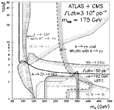
Figure 13: Reach of LHC to discover one or more of the particles in the minimal SUSY Higgs sector. Assumes an integrated luminosity of $3\times 10^{4}$ pb^-1 and 2-detectors. Note that there is a slight “hole” for $m_{A}\sim 250$ GeV and $\tan\beta\sim 6$. From [83].

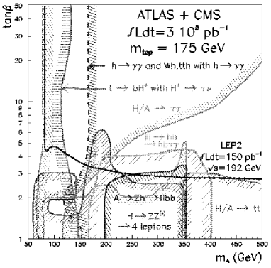
Figure 14: Same as Fig. 13, but assuming an integrated luminosity of $3\times 10^{5}$ pb^-1. Note that the “hole” for $m_{A}\sim 250$ GeV and $\tan\beta\sim 6$ in the previous figure is now covered. From [83].

While the results in Fig. 13 and (especially) Fig. 14 are reassuring, the difficult issues will be to distinguish this signal from that of the standard Higgs. This is particularly a problem in the large-$m_{A}$ region where the decoupling-limit insures that the couplings of the $h^{0}$ are identical to those of the standard Higgs. Establishing the minimal SUSY model will certainly require the discovery of superpartners, in addition to an exploration of the symmetry breaking sector.

8 Dynamical Electroweak Symmetry Breaking

1 Technicolor

The simplest theory of dynamical electroweak symmetry breaking is technicolor [79, 80]. Consider an $SU(N_{TC})$ gauge theory with fermions in the fundamental representation of the gauge group

$$\Psi_{L}=\left(\begin{array}[]{c}U\\ D\end{array}\right)_{L}\,\,\,\,\,\,\,\,U_{R},D_{R}$$ (95)

The fermion kinetic energy terms for this theory are

$${\cal L} = \bar{U}_{L}i\hbox to0.0pt{\hbox to8.55695pt{\hfil/\hfil}\hss}DU_{L}+\bar{U}_{R}i\hbox to0.0pt{\hbox to8.55695pt{\hfil/\hfil}\hss}DU_{R}+$$

$$\bar{D}_{L}i\hbox to0.0pt{\hbox to8.55695pt{\hfil/\hfil}\hss}DD_{L}+\bar{D}_{R}i\hbox to0.0pt{\hbox to8.55695pt{\hfil/\hfil}\hss}DD_{R}~{},$$

and, like QCD in the $m_{u}$, $m_{d}\to 0$ limit, they have a chiral $SU(2)_{L}\times SU(2)_{R}$ symmetry.

As in QCD, exchange of technigluons in the spin zero, isospin zero channel is attractive causing the formation of a condensate

$${\lower 15.0pt\hbox{ \epsfbox{figures/qqbar.ps}}\ \ \rightarrow\ \ \langle\bar{U}_{L}U_{R}\rangle=\langle\bar{D}_{L}D_{R}\rangle\neq 0\,,}$$ (97)

which dynamically breaks $SU(2)_{L}\times SU(2)_{R}\to SU(2)_{V}$. These broken chiral symmetries imply the existence of three massless Goldstone bosons, the analogs of the pions in QCD.

Now consider gauging $SU(2)_{W}\times U(1)_{Y}$ with the left-handed fermions transforming as weak doublets and the right-handed ones as weak singlets. To avoid gauge anomalies, in this one-doublet technicolor model we will take the left-handed technifermions to have hypercharge zero and the right-handed up- and down-technifermions to have hypercharge $\pm 1/2$. The spontaneous breaking of the chiral symmetry breaks the weak-interactions down to electromagnetism. The would-be Goldstone bosons become the longitudinal components of the $W$ and $Z$

$$\pi^{\pm},\,\pi^{0}\,\rightarrow\,W^{\pm}_{L},\,Z_{L}~{},$$ (98)

which acquire a mass

$$M_{W}={gF_{TC}\over 2}~{}.$$ (99)

Here $F_{TC}$ is the analog of $f_{\pi}$ in QCD. In order to obtain the experimentally observed masses, we must have that $F_{TC}\approx 246{\rm GeV}$ and hence this model is essentially QCD scaled up by a factor of

$${F_{TC}\over f_{\pi}}\approx 2500\,.$$ (100)

While I have described only the simplest model above, from the discussion of section 5.1 (see fig. 9) it is straightforward to generalize to other cases. Any strongly interacting gauge theory with a chiral symmetry breaking pattern $G\to H$, in which $G$ contains $SU(2)_{W}\times U(1)_{Y}$ and breaks to a subgroup $H\supset U(1)_{em}$ (with $SU(2)_{W}\times U(1)_{Y}\not\subset H$) will break the weak interactions down to electromagnetism. In order to be consistent with experimental results, however, we must also require that $H$ contain “custodial” $SU(2)_{C}$. This custodial symmetry insures that the $F$-constant associated with the $W^{\pm}$ and $Z$ are equal and therefore that the relation

$$\rho={M_{W}\over M_{Z}\sin\theta_{W}}=1$$ (101)

is satisfied at tree-level. If the chiral symmetry is larger than $SU(2)_{L}\times SU(2)_{R}$, theories of this sort will contain additional (pseudo-)Goldstone bosons which are not “eaten” by the $W$ and $Z$. For simplicity, in this lecture we will discuss the phenomenology of the one-doublet model.

2 The Phenomenology of Dynamical Electroweak Symmetry Breaking

Of the particles that we have observed to date, the only ones directly related to the electroweak symmetry breaking sector are the longitudinal gauge-bosons. Therefore, we expect the most direct signatures for electroweak symmetry breaking to come from the scattering of longitudinally gauge bosons. As discussed in section 2, at high energies, we may use the equivalence theorem [19, 20, 21]

$${\cal A}(W_{L}W_{L})={\cal A}(\pi\pi)+{\cal O}({M_{W}\over E})\,.$$ (102)

to reduce the problem of longitudinal gauge boson ($W_{L}$) scattering to the corresponding (and generally simpler) problem of the scattering of the Goldstone bosons ($\pi$) that would be present in the absence of the weak gauge interactions.

In order to correctly describe the weak interactions, the symmetry breaking sector must have an (at least approximate) custodial symmetry [79, 80, 6], and the most general effective theory describing the behavior of the Goldstone bosons is an effective chiral lagrangian with an $SU(2)_{L}\times SU(2)_{R}\to SU(2)_{V}$ symmetry breaking pattern. This effective lagrangian is most easily written in terms of a field

$$\Sigma=\exp(i\pi^{a}\sigma^{a}/F_{TC})~{},$$ (103)

where the $\pi^{a}$ are the Goldstone boson fields, the $\sigma^{a}$ are the Pauli matrices, and where the field $\Sigma$ which transforms as

$$\Sigma\to L\Sigma R^{\dagger}$$ (104)

under $SU(2)_{L}\times SU(2)_{R}$.

The interactions can then be ordered in a power-series in momenta. Allowing for custodial $SU(2)$ violation, the lowest-order terms in the effective theory are the gauge-boson kinetic terms

$$-{1\over 2}{\rm Tr}\left[{\rm\bf W}^{\mu\nu}{\rm\bf W}_{\mu\nu}\right]-{1\over 2}{\rm Tr}\left[{\rm\bf B}^{\mu\nu}{\rm\bf B}_{\mu\nu}\right]\,,$$ (105)

and the ${\cal O}(p^{2})$ terms

$${{F_{TC}^{2}\over 4}{\rm Tr}\left[D^{\mu}\Sigma^{\dagger}D_{\mu}\Sigma\right]+{F_{TC}^{2}\over 2}({1\over\rho}-1)\left[{\rm Tr}T_{3}\Sigma^{\dagger}D^{\mu}\Sigma\right]^{2}}\,,$$ (106)

where

$$D_{\mu}\Sigma=\partial_{\mu}\Sigma+{\rm i}g{\rm\bf W}_{\mu}\Sigma-{\rm i}\Sigma g^{\prime}{\rm\bf B}_{\mu}~{}.$$ (107)

In unitary gauge, $\Sigma=1$ and the lowest-order terms in eq. (106) give rise to the $W$ and $Z$ masses

$${g^{2}F_{TC}^{2}\over 4}W^{-\mu}W^{+}_{\mu}+{g^{2}F_{TC}^{2}\over{8\rho\cos^{2}\theta}}Z^{\mu}Z_{\mu}~{}.$$ (108)

So far, the description we have constructed is valid in any theory of electroweak symmetry breaking. The interactions in eq. (106) result in universal low-energy [17, 18] theorems shown in eq. (24). These amplitudes increase with energy and, at some point, this growth must stop [15, 16]. What dynamics cuts off growth in these amplitudes? In general, there are three possibilities:

• new particles

• the born approximation fails $\rightarrow$ strong interactions

• both.

Figure 15: QCD data [85]and low-energy theorem (solid line) prediction for the magnitude of the spin-1/isospin-1 pion scattering amplitude $|a_{F1}|$.

In the case of QCD-like technicolor, we take our inspiration from the familiar strong interactions. The data for $\pi\pi$ scattering in QCD in the $I=J=1$ channel is shown in Figure 15. After correcting for the finite pion mass, we see that the scattering amplitude follows the low-energy prediction near threshold, but at higher energies the amplitude is dominated by the $\rho$-meson whose appearance both enhances the scattering cross-section and cuts-off the growth of the scattering amplitude at higher energies. In a QCD-like technicolor theory, then, we expect the appearance of a vector meson whose mass we estimate by scaling by $F_{TC}/f_{\pi}\approx 2500$. That is,

$$M_{\rho_{TC}}\approx 2{\rm\,TeV}\,\sqrt{3\over N_{TC}}~{},$$ (109)

where we have included large-$N_{TC}$ scaling to estimate the effect of $N_{TC}\neq 3$ [86].

The appearance of these technivector mesons would provide the most direct experimental signature of dynamical electroweak symmetry breaking. At the LHC, gauge boson scattering occurs through the following process,

$${\lower 20.0pt\hbox{{\epsfbox{figures/vvscatt.eps}}}}~{},$$ (110)

and would receive contributions from technivector meson exchange. Note that, in addition to high-$p_{T}$ gauge bosons, one expects forward “tag” jets (with a typical transverse momentum of order $M_{W}$) from the quarks which radiate the initial gauge bosons. The signal expected is shown [87, 88] in Figure 16 for $M_{\rho_{TC}}=1.0\,{\rm\,TeV},2.5\,{\rm\,TeV}$. Note the scale: events per 50 GeV bin of transverse mass ($M_{T}$) per 100 fb^-1!

    

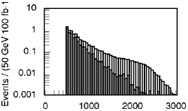
Figure 16: Gauge boson scattering signal plus background (grey) and background (black) for $W^{\pm}Z$ production [87, 88] at LHC for technirho masses of 1.0 TeV and 2.5 TeV. Signal selection requirements shown in table above.

An additional signal is provided through the technicolor analog of “vector-meson dominance.” In particular, the $W$ and $Z$ can mix with the technirho mesons in a manner exactly analogous to $\gamma$-$\rho$ mixing in QCD:

$${\lower 5.0pt\hbox{{\epsfbox{figures/vacpol.eps}}}}\hskip 5.0pt\rightarrow\hskip 5.0pt{\lower 15.0pt\hbox{{\epsfbox{figures/qqmix.eps}}}}~{}.$$ (111)

Note that this process does not have a very forward jet and is distinguishable from the gauge boson scattering signal discussed above. The vector-meson mixing signal [89] at the LHC is shown in Figure 17 for $M_{\rho_{TC}}=1.0\,{\rm\,TeV},2.5\,{\rm\,TeV}$.

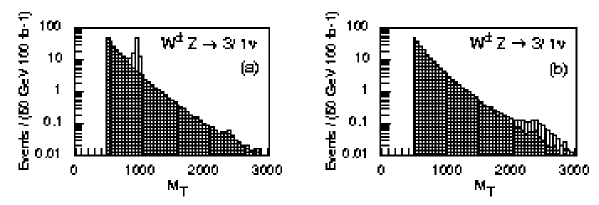
Figure 17: Vector meson mixing signal plus background (grey) and background (black) for $W^{\pm}Z$ production [89] at LHC for technirho masses of (a) 1.0 TeV and (b) 2.5 TeV.

A dynamical electroweak symmetry breaking sector will also have affect two gauge-boson production at a high-energy $e^{+}e^{-}$ collider such as the NLC. For example, if gauge-boson re-scattering 

(112)

is dominated by a technirho meson, it can be parameterized in terms of a $ZWW$ form-factor

$$F_{T}=\exp\bigl{[}{1\over\pi}\int_{0}^{\infty}ds^{\prime}\delta(s^{\prime},M_{\rho},\Gamma_{\rho})\{{1\over s^{\prime}-s-i\epsilon}-{1\over s^{\prime}}\}\bigr{]}~{},$$ (113)

where

$$\delta(s)={1\over 96\pi}{s\over v^{2}}+{3\pi\over 8}\left[\tanh({s-M_{\rho}^{2}\over M_{\rho}\Gamma_{\rho}})+1\right]~{}.$$ (114)

This two gauge-boson production mechanism interferes with continuum production, and by an accurate measurement of the decay products it is possible [93] to reconstruct the real and imaginary parts of the form-factor $F_{T}$. The expected accuracy of a 500 GeV NLC with 80 fb^-1 is shown in Figure 18.

Figure 18: $ZWW$ form-factor measurement [93] at a 500 GeV NLC with 80fb^-1. Predictions are shown for the standard model, and for technicolor for various technirho masses.

3 Low-Energy Phenomenology

Even though the most direct signals of a dynamical electroweak symmetry breaking sector require (partonic) energies of order 1 TeV, there are also effects which may show up at lower energies as well. While the ${\cal O}(p^{2})$ terms in the effective lagrangian are universal, terms of higher order are model-dependent. At energies below $M_{\rho_{TC}}$, there are corrections to 3-pt functions:

$${\lower 15.0pt\hbox{\epsfbox{figures/agvtc.eps}}}~{},$$ (115)

which, following Gasser and Leutwyler [50, 51, 94, 95, 96], give rise to the O($p^{4}$) terms

$$-\ ig{{\it l}_{9L}\over 16\pi^{2}}\,{\rm Tr}{{\rm\bf W}^{\mu\nu}D_{\mu}\Sigma D_{\nu}\Sigma^{\dagger}}~{},$$ (116)

and

$$-\ ig^{\prime}{{\it l}_{9R}\over 16\pi^{2}}\,{\rm Tr}{{\rm\bf B}^{\mu\nu}D_{\mu}\Sigma^{\dagger}D_{\nu}\Sigma}~{}.$$ (117)

There are also corrections to the 2-pt functions:

(118)

which give rise to

$$\ +\ gg^{\prime}{{\it l}_{10}\over 16\pi^{2}}\,{\rm Tr}{\Sigma{\rm\bf B}^{\mu\nu}\Sigma^{\dagger}{\rm\bf W}_{\mu\nu}}~{}.$$ (119)

In these expressions, the l’s are normalized to be O(1).

The corrections to the 3-point functions are typically parameterized, following Hagiwara, et. al. [97], parameterized as:

$${i\over e\cot\theta} {\cal L}_{WWZ}=g_{1}(W^{\dagger}_{\mu\nu}W^{\mu}Z^{\nu}-W^{\dagger}_{\mu}Z_{\nu}W^{\mu\nu})$$ (120)

$$+\kappa_{Z}W^{\dagger}_{\mu}W_{\nu}Z^{\mu}\nu+{\lambda_{Z}\over M_{W}^{2}}W^{\dagger}_{\lambda\mu}W^{\mu}_{\nu}Z^{\nu\lambda}~{},$$

and

$${i\over e} {\cal L_{WW\gamma}}=(W^{\dagger}_{\mu\nu}W^{\mu}A^{\nu}-W_{\mu}^{\dagger}A_{\nu}W^{\mu\nu})$$ (121)

$$+\kappa_{\gamma}W^{\dagger}_{\mu}W_{\nu}F^{\mu}\nu+{\lambda_{\gamma}\over M_{W}^{2}}W^{\dagger}_{\lambda\mu}W^{\mu}_{\nu}F^{\nu\lambda}~{}.$$

Re-expressing these coefficients in terms of the parameters in ${\cal L}_{p^{4}}$ given above, we find

$$\left.\begin{array}[]{c}g_{1}-1\\ \kappa_{Z}-1\\ \kappa_{\gamma}-1\end{array}\right\}\ \approx\ {\alpha_{*}l_{i}\over 4\pi\sin^{2}\theta}={\cal O}(10^{-2}-10^{-3})~{},$$ (122)

and $\lambda_{Z,\gamma}$ from ${\cal L}_{p^{6}}$ implying that

$$\lambda_{Z,\gamma}={\cal O}(10^{-4}-10^{-5})\,.$$ (123)

The best current limits [98], coming from Tevatron experiments, are shown in Figure 19. Unfortunately, they do not reach the level of sensitivity required. The situation [98] is somewhat improved at the LHC, as shown in Figure 20, or at a 500 or 1500 GeV NLC, as shown in Figure 21.

    

Figure 19: Current limits [98] on anomalous gauge-boson vertices from Tevatron data.

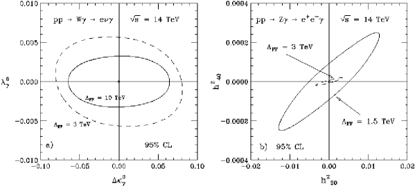
Figure 20: Experimental [98] reach of LHC to probe anomalous gauge-boson vertices given an integrated luminosity of 100 fb^-1.

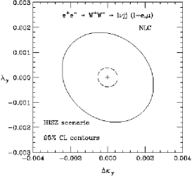
Figure 21: Experimental [98] reach of a 500 GeV (solid) or 1500 GeV (dashed) NLC to probe anomalous gauge-boson vertices, assuming 80 fb^-1 or 190 fb^-1 respectively.

The corrections [99, 100, 101, 102, 103] to the 2-point functions give rise to contributions to the “oblique parameters” $S$

$$S \equiv 16\pi\left[\Pi^{\prime}_{33}(0)-\Pi^{\prime}_{3Q}(0)\right]$$ (124)

$$= -\pi{\it l}_{10}\approx 4\pi\left({F^{2}_{\rho_{TC}}\over M^{2}_{\rho_{TC}}}-{F^{2}_{A_{TC}}\over M^{2}_{A_{TC}}}\right)N_{D}~{},$$

and $T$

$$\alpha T\equiv{g^{2}\over{\cos^{2}\theta M_{Z}^{2}}}\left[\Pi_{11}(0)-\Pi_{33}(0)\right]=\rho-1~{}.$$ (125)

$S$ and $T$ measure the size of custodial-symmetry conserving and violating radiative corrections to the gauge boson propagators beyond the corrections present in the standard model. Current experimental constraints [104] imply the bounds shown in Figure 22, at 95% confidence level for different values of $\alpha_{S}$. Scaling from QCD, we expect a contribution to S of order

$$S\approx 0.28N_{D}(N_{TC}/3)~{},$$ (126)

for an $SU(N_{TC})$ technicolor theory with $N_{D}$ technidoublets. From these we see that, with the possible exception of $N_{D}=1$ and $N_{TC}=2$ or 3, QCD-like technicolor is in conflict with precision weak measurements.

Figure 22: 90% confidence level bounds [104] on the oblique parameters $S$ and $T$ for $\alpha_{S}=0.115$ (solid) and 0.124 (dashed).

In summary, dynamical electroweak symmetry breaking provides a natural and attractive mechanism for producing the $W$ and $Z$ masses. Generically models of this type predict strong $WW$-Scattering, signals of which may be observable at the LHC. While the simplest QCD-like models serve as a useful starting point, they are excluded (except, perhaps, for an $SU(2)_{TC}$ model with one doublet) since they would give rise to unacceptably large contributions to the $S$ parameter. In the next section we will discuss the additional interactions and features required in more realistic models to give rise to the masses to the ordinary fermions.

9 Flavor Symmetry Breaking and ETC

1 Fermion Masses & ETC Interactions

In order to give rise to masses for the ordinary quarks and leptons, we must introduce interactions which connect the chiral-symmetries of technifermions to those of the ordinary fermions. The most popular choice [56, 57] is to introduce new broken gauge interactions, called extended technicolor interactions (ETC), which couple technifermions to ordinary fermions. At energies low compared to the ETC gauge-boson mass, $M_{ETC}$, these effects can be treated as local four-fermion interactions

$${\lower 15.0pt\hbox{\epsfbox{figures/etc.eps}}}\ \ \rightarrow\ \ {{g_{ETC}^{2}\over M^{2}_{ETC}}}(\overline{\Psi}_{L}U_{R})({\overline{q}_{R}q_{L}})~{}.$$ (127)

After technicolor chiral-symmetry breaking and the formation of a $\langle\bar{U}U\rangle$ condensate, such an interaction gives rise to a mass for an ordinary fermion

$$m_{q}\approx{{g_{ETC}^{2}\over M^{2}_{ETC}}}\langle\overline{U}U\rangle_{ETC}~{},$$ (128)

where $\langle\overline{U}U\rangle_{ETC}$ is the value of the technifermion condensate evaluated at the ETC scale (of order $M_{ETC}$). The condensate renormalized at the ETC scale in eq. (128) can be related to the condensate renormalized at the technicolor scale as follows

$$\langle\overline{U}U\rangle_{ETC}=\langle\overline{U}U\rangle_{TC}\exp\left(\int_{\Lambda_{TC}}^{M_{ETC}}{d\mu\over\mu}\gamma_{m}(\mu)\right)~{},$$ (129)

where $\gamma_{m}(\mu)$ is the anomalous dimension of the fermion mass operator and $\Lambda_{TC}$ is the analog of $\Lambda_{QCD}$ for the technicolor interactions.

For QCD-like technicolor (or any theory which is “precociously” asymptotically free), $\gamma_{m}$ is small over in the range between $\Lambda_{TC}$ and $M_{ETC}$ and using dimensional analysis [50, 94, 51, 95, 96] we find

$$\langle\overline{U}U\rangle_{ETC}\approx\langle\overline{U}U\rangle_{TC}\approx 4\pi F^{3}_{TC}~{}.$$ (130)

In this case eq. (128) implies that

$${{M_{ETC}\over g_{ETC}}}\approx 40{\rm\,TeV}\left({F_{TC}\over 250{\rm\,GeV}}\right)^{3\over 2}\left({100{\rm\,MeV}\over m_{q}}\right)^{1\over 2}~{}.$$ (131)

In order to orient our thinking, it is instructive to consider a simple “toy” extended technicolor model. The model is based on an $SU(N_{ETC})$ gauge group, with technicolor as an extension of flavor. In this case $N_{ETC}=N_{TC}+N_{F}$, and we add the (anomaly-free) set of fermions

$\begin{array}[]{l@{\extracolsep{15pt}}l}Q_{L}=(N_{ETC},3,2)_{1/6}&L_{L}=(N_{ETC},1,2)_{-1/2}\\ U_{R}=(N_{ETC},3,1)_{2/3}&E_{R}=(N_{ETC},1,1)_{-1}\\ D_{R}=(N_{ETC},3,1)_{-1/3}&N_{R}=(N_{ETC},1,1)_{0}~{},\end{array}$

where we display their quantum numbers under $SU(N_{ETC})\times SU(3)_{C}\times SU(2)_{W}\times U(1)_{Y}$. We break the ETC group down to technicolor in three stages

$SU(N_{TC}+3)$

$\Lambda_{1}\ \ \ \ \ \downarrow\ \ \ \ \ m_{1}\approx{4\pi F^{3}\over\Lambda^{2}_{1}}$

$SU(N_{TC}+2)$

$\Lambda_{2}\ \ \ \ \ \downarrow\ \ \ \ \ m_{2}\approx{4\pi F^{3}\over\Lambda^{2}_{2}}$

$SU(N_{TC}+1)$

$\Lambda_{3}\ \ \ \ \ \downarrow\ \ \ \ \ m_{3}\approx{4\pi F^{3}\over\Lambda^{2}_{3}}$

$SU(N_{TC})$

resulting in three isospin-symmetric families of degenerate quarks and leptons, with $m_{1}<m_{2}<m_{3}$. Note that the heaviest family is related to the lightest ETC scale!

Before continuing our general discussion, it is worth noting a couple of points. First, in this example the ETC gauge bosons do not carry color or weak charge

$$[G_{ETC},SU(3)_{C}]=[G_{ETC},SU(2)_{W}]=0~{}.$$ (132)

Furthermore, in this model there is one technifermion for each type of ordinary fermion: that is, this is a “one-family” technicolor model [105]. Since there are eight left- and right- handed technifermions, the chiral symmetry of the technicolor theory is (in the limit of zero QCD and weak couplings) $SU(8)_{L}\times SU(8)_{R}\to SU(8)_{V}$. Such a theory would yield $8^{2}-1=63$ (pseudo-)Goldstone bosons. Three of these Goldstone bosons are unphysical — the corresponding degrees of freedom become the longitudinal components of the $W^{\pm}$ and $Z$ by the Higgs mechanism. The remaining 60 must somehow obtain a mass. This will lead to the condition in eq. (132) being modified in a realistic model. We will return to the issue of pseudo-Goldstone bosons below.

The most important feature of this or any ETC-model is that a successful extended technicolor model will provide a dynamical theory of flavor! As in the toy model described above and as explicitly shown in eq. (127) above, the masses of the ordinary fermions are related to the masses and couplings of the ETC gauge-bosons. A successful and complete ETC theory would predict these quantities and, hence, the ordinary fermion masses.

Needless to say, constructing such a theory is very difficult. No complete and successful theory has been proposed. Examining our toy model, we immediately see a number of shortcomings of this model that will have to be addressed in a more realistic theory:

• What breaks ETC?

• Do we require a separate scale for each family?

• How do the $T_{3}=\pm{1\over 2}$ fermions of a given generation receive different masses?

• How do we obtain quark mixing angles?

• What about right-handed technineutrinos and $m_{\nu}$?

2 Flavor-Changing Neutral-Currents

Perhaps the single biggest obstacle to constructing a realistic ETC model (or any dynamical theory of flavor) is the potential for flavor-changing neutral currents [56]. Quark mixing implies transitions between different generations: $q\to\Psi\to q^{\prime}$, where $q$ and $q^{\prime}$ are quarks of the same charge from different generations and $\Psi$ is a technifermion. Consider the commutator of two ETC gauge currents:

$$[\overline{q}\gamma\Psi,\overline{\Psi}\gamma q^{\prime}]\,\supset\,\overline{q}\gamma q^{\prime}\,.$$ (133)

Hence we expect there are ETC gauge bosons which couple to flavor-changing neutral currents. In fact, this argument is slightly too slick: the same applies to the charged-current weak interactions! However in that case the gauge interactions, $SU(2)_{W}$ respect a global $(SU(5)\times U(1))^{5}$ chiral symmetry [106] leading to the usual GIM mechanism.

Unfortunately, the ETC interactions cannot respect GIM exactly; they must distinguish between the various generations in order to give rise to the masses of the different generations. Therefore, flavor-changing neutral-current interactions are (at least at some level) unavoidable.

The most severe constraints come from possible $|\Delta S|=2$ interactions which contribute to the $K_{L}$-$K_{S}$ mass difference. In particular, we would expect that in order to produce Cabibbo-mixing the same interactions which give rise to the $s$-quark mass could cause the flavor-changing interaction

$${\cal L}_{|\Delta S|=2}={g^{2}_{ETC}\,\theta^{2}_{sd}\over{M^{2}_{ETC}}}\,\,\left(\overline{s}\Gamma^{\mu}d\right)\,\,\left(\overline{s}\Gamma^{\prime}_{\mu}d\right)+{\rm h.c.}~{},$$ (134)

where $\theta_{sd}$ is of order the Cabibbo angle. Such an interaction contributes to the neutral kaon mass splitting

$$(\Delta M^{2}_{K})_{ETC}={g^{2}_{ETC}\,\theta^{2}_{sd}\over{M^{2}_{ETC}}}\,\langle\overline{K^{0}}|\overline{s}\Gamma^{\mu}d\,\overline{s}\Gamma^{\prime}_{\mu}d|K^{0}\rangle+{\rm c.c.}$$ (135)

Using the vacuum insertion approximation we find

$$(\Delta M^{2}_{K})_{ETC}\simeq{g^{2}_{ETC}\,{\rm Re}(\theta^{2}_{sd})\over{2M^{2}_{ETC}}}\,f^{2}_{K}M^{2}_{K}~{}.$$ (136)

Experimentally we know that $\Delta M_{K}<3.5\times 10^{-12}\,{\rm\,MeV}$ and, hence, that

$${M_{ETC}\over{g_{ETC}\,\sqrt{{\rm Re}(\theta^{2}_{sd})}}}>600\,{\rm\,TeV}$$ (137)

Using eq. (128) we find that

$$m_{q,\ell}\simeq{g_{ETC}^{2}\over{M_{ETC}^{2}}}\langle\overline{T}T\rangle_{ETC}<{0.5\,{\rm\,MeV}\over{N_{D}^{3/2}\,\theta_{sd}^{2}}}\,$$ (138)

showing that it will be difficult to produce the $s$-quark mass, let alone the $c$-quark!

3 Pseudo-Goldstone Bosons

As illustrated by our toy model above, a “realistic” ETC theory may require a technicolor sector with a chiral symmetry structure bigger than the $SU(2)_{L}\times SU(2)_{R}$ discussed in detail in the previous lecture. The prototypical model of this sort is the one-family model incorporated in our toy model. As discussed there, the theory has an $SU(8)_{L}\times SU(8)_{R}\to SU(8)_{V}$ chiral symmetry breaking structure resulting in 63 Goldstone bosons, 3 of which are unphysical. The quantum numbers of the 60 remaining Goldstone bosons are shown in table 1. Clearly, these objects cannot be massless in a realistic theory!

Table 1: Quantum numbers of the 60 physical Goldstone bosons (and the corresponding vector mesons) in a one-family technicolor model. Note that the mesons that transform as 3’s of QCD are complex fields.

SU$(3)_{C}$	SU$(2)_{V}$	Particle
$1$	$1$	$P^{0\prime}\;,\;\omega_{T}$
$1$	$3$	$P^{0,\pm}\;,\;\rho^{0,\pm}_{T}$
$3$	$1$	$P^{0\prime}_{3}\;,\;\rho^{0\prime}_{T3}$
$3$	$3$	$P^{0,\pm}_{3}\;,\;\rho^{0,\pm}_{T3}$
$8$	$1$	$P^{0\prime}_{8}(\eta_{T})\;,\;\rho^{0\prime}_{T8}$
$8$	$3$	$P^{0,\pm}_{8}\;,\;\rho^{0,\pm}_{T8}$

In fact, the ordinary gauge interactions break the full $SU(8)_{L}\times SU(8)_{R}$ chiral symmetry explicitly. The largest effects are due to QCD and the color octets and triplets mesons get masses of order 200 – 300 GeV, in analogy to the electromagnetic mass splitting $m_{\pi^{+}}-m_{\pi^{0}}$ in QCD. Unfortunately, the others [56] are massless to O($\alpha$)!

Luckily, the ETC interactions (which we introduced in order to give masses to the ordinary fermions) are capable of explicitly breaking the unwanted chiral symmetries and producing masses for these mesons. This is because in addition to coupling technifermions to ordinary fermions, some ETC interactions also couple technifermions to themselves [56]. Using Dashen’s formula [107], we can estimate that such an interaction can give rise to an effect of order

$$F^{2}_{TC}M^{2}_{\pi_{T}}\propto{g^{2}_{ETC}\over M^{2}_{ETC}}\langle(\overline{T}T)^{2}\rangle_{ETC}~{}.$$ (139)

In the vacuum insertion approximation for a theory with small $\gamma_{m}$, we may rewrite the above formula using eq. (128) and find that

$$M_{\pi_{T}}\simeq 55{\rm\,GeV}\sqrt{m_{f}\over 1{\rm\,GeV}}\sqrt{250{\rm\,GeV}\over F_{TC}}~{}.$$ (140)

It is unclear that this large enough.

In addition, there is a particularly troubling chiral symmetry in the one-family model. The $SU(8)$-current $\overline{Q}\gamma_{\mu}\gamma_{5}Q-3\overline{L}\gamma_{\mu}\gamma_{5}L$ is spontaneously broken and has a color anomaly. Therefore, we have a potentially dangerous weak scale axion [67, 68, 69, 70]! An ETC-interaction of the form

$${g^{2}_{ETC}\over M^{2}_{ETC}}\left(\overline{Q}_{L}\gamma^{\mu}L_{L}\right)\left(\overline{L}_{R}\gamma^{\mu}Q_{R}\right)~{},$$ (141)

is required to give to an axion mass, and we must [56] embed $SU(3)_{C}$ in $ETC$.

Finally, before moving on I would like to note that there is an implicit assumption in the analysis of gauge-boson scattering presented in the last section. We have assumed that elastic scattering dominates. In the presence of many pseudo-Goldsone bosons, $WW$ scattering could instead be dominated by inelastic scattering. This effect has been illustrated [108] in an $O(N)$-Higgs model with many pseudo-Goldstone Bosons, solved in large-N limit. Instead of the expected resonance structure at high energies, the scattering can be small and structureless at all energies.

4 ETC etc.

There are other model-building constraints [109] on a realistic TC/ETC theory. A realistic ETC theory:

• must be asymptotically free,

• cannot have gauge anomalies,

• must produce small (or zero) neutrino masses,

• cannot give rise to extra massless (or even light) gauge bosons,

• should generate weak CP-violation without producing unacceptably large amounts of strong CP-violation,

• must give rise to isospin-violation in fermion masses without large contributions to $\Delta\rho$ and,

• must accomodate a large $m_{t}$ while giving rise to only small corrections to $Z\to\overline{b}b$ and $b\to s\gamma$.

Clearly, building a fully realistic ETC model will be quite difficult! However, as I have emphasized before, this is because an ETC theory must provide a complete dynamical explanation of flavor. In the next section, I will concentrate on possible solutions to the flavor-changing neutral-current problem(s). As I will discuss in detail in sections 11 and 12, I believe the outstanding obstacle in ETC or any theory of flavor is providing an explanation for the top-quark mass, i.e. dealing with the last three issues listed above.

5 Technicolor with a Scalar

At this point, it would be easy to believe that it is impossible to construct a model of dynamical electroweak symmetry breaking. Fortunately, there is at least an existence [110, 111, 112] proof of such a theory: technicolor with a scalar. Admittedly, while electroweak symmetry breaking has a dynamical origin in this theory, the introduction of a scalar reintroduces the hierarchy and naturalness problems we had originally set out to solve.

In the simplest model one starts with a one doublet technicolor theory, and couples the chiral-symmetries of technifermions to ordinary fermions through scalar exchange:

(142)

The phenomenology of this model has been studied in detail [118], and the allowed region is shown in Figure 23.

Figure 23: Plot of allowed parameter space in model of technicolor with a scalar [119]. $h$ is the Yukawa coupling of the scalar to technifermions and $\tilde{M}_{\phi}$ is the neutral scalar mass. The “triangular” region formed by the solid and dashed lines is allowed.

10 Walking Technicolor

1 The Gap Equation

Up to now we have assumed that technicolor is, like QCD, precociously asymptotically free and $\gamma_{m}(\mu)$ is small for $\Lambda_{TC}<\mu<M_{ETC}$. However, as discussed above it is difficult to construct an ETC theory of this sort without producing dangerously large flavor-changing neutral currents. On the other hand, if $\beta_{TC}$ is small, $\alpha_{TC}$ can remain large above the scale $\Lambda_{TC}$ — i.e. the technicolor coupling would “walk” instead of running. In this same range of momenta, $\gamma_{m}$ may be large and, since

$$\langle\overline{T}T\rangle_{ETC}=\langle\overline{T}T\rangle_{TC}\exp\left(\int_{\Lambda_{TC}}^{M_{ETC}}{d\mu\over\mu}\gamma_{m}(\mu)\right)$$ (143)

this could enhance $\langle\overline{T}T\rangle_{ETC}$ and fermion masses [120, 121, 122, 123, 124, 125].

Figure 24: Schwinger-Dyson equation for the fermion self-energy function $\Sigma(p)$ in the rainbow approximation.

In order to proceed further, however, we need to understand how large $\gamma_{m}$ can be and how walking affects the technicolor chiral symmetry breaking dynamics. These questions cannot be addressed in perturbation theory. Instead, what is conventionally done is to use a nonperturbative aproximation for $\gamma_{m}$ and chiral-symmetry breaking dynamics based on the “rainbow” approximation [126, 127] to the Schwinger-Dyson equation shown in Figure 24. Here we write the full, nonperturbative, fermion propagator in momentum space as

$$iS^{-1}(p)=Z(p)(\hbox to0.0pt{\hbox to5.03125pt{\hfil/\hfil}\hss}p-\Sigma(p))~{}.$$ (144)

The linearized form of the gap equation in Landau gauge (in which $Z(p)\equiv 1$ in the rainbow approximation) is

$$\Sigma(p)=3C_{2}(R)\,\int{d^{4}k\over{(2\pi)^{4}}}\,{\alpha_{TC}((k-p)^{2})\over{(k-p)^{2}}}\,{\Sigma(k)\over{k^{2}}}~{}.$$ (145)

Being separable, this integral equation can be converted to a differential equation which has the approximate (WKB) solutions [128, 129]

$$\Sigma(p)\propto p^{-\gamma_{m}(\mu)}\,,\,\,p^{\gamma_{m}(\mu)-2}\,.$$ (146)

Here $\alpha(\mu)$ is assumed to run slowly, as will be the case in walking technicolor, and the anomalous dimension of the fermion mass operator is

$$\gamma_{m}(\mu)=1-\sqrt{1-{\alpha_{TC}(\mu)\over\alpha_{C}}}\,;\ \ \alpha_{C}\equiv{\pi\over 3C_{2}(R)}\,.$$ (147)

One can give a physical interpretation of these two solutions [130, 131]. Using the operator product expansion, we find

$$\lim_{p\to\infty}\Sigma(p)\ \ \propto\ \ \lower 15.0pt\hbox{\epsfbox{figures/ope.eps}}~{},$$ (148)

and hence the first solution corresponds to a “hard mass” or explicit chiral symmetry breaking, while the second solution corresponds to a “soft mass” or spontaneous chiral symmetry breaking. If we let $m_{0}$ be the explicit mass of a fermion, dynamical symmetry breaking occurs only if

$$\lim_{m_{0}\to 0}\Sigma(p)\neq 0\,.$$ (149)

A careful analysis of the gap equation, or equivalently the appropriate effective potential [132], implies that this happens only if $\alpha_{TC}$ reaches a critical value of chiral symmetry breaking, $\alpha_{C}$ defined in eq. (147). Furthermore, the chiral symmetry breaking scale $\Lambda_{TC}$ is defined by the scale at which

$$\alpha_{TC}(\Lambda_{TC})=\alpha_{C}$$ (150)

and hence, at least in the rainbow approximation, at which

$$\gamma_{m}(\Lambda_{TC})=1.$$ (151)

In the rainbow approximation, then, chiral symmetry breaking occurs when the “hard” and “soft” masses scale the same way. It is believed that even beyond the rainbow approximation $\gamma_{m}=1$ at the critical coupling [133, 134, 135].

2 Implications of Walking: Fermion and PGB Masses, $S$

If $\beta(\alpha_{TC})\simeq 0$ all the way from $\Lambda_{TC}$ to $M_{ETC}$, then $\gamma_{m}(\mu)\cong 1$ in this range. In this case, eq. (128) becomes

$$m_{q,l}={g^{2}_{ETC}\over{M^{2}_{ETC}}}\times\left(\langle\overline{T}T\rangle_{ETC}\cong\langle\overline{T}T\rangle_{TC}\,{M_{ETC}\over{\Lambda_{TC}}}\right)~{}.$$ (152)

We have previously estimated that flavor-changing neutral current requirements imply that the ETC scale associated with the second generation must be greater than of order 100 to 1000 TeV. In the case of walking technicolor the enhancement of the technifermion condensate implies that

$$m_{q,l}\simeq{{50\,-\,500{\rm\,MeV}}\over N^{3/2}_{D}\theta^{2}_{sd}}~{},$$ (153)

arguably enough to accomodate the strange and charm quarks.

While this is very encouraging, two caveats should be kept in mind. First, the estimates given are for limit of “extreme walking”, i.e. assuming that the technicolor coupling walks all the way from the technicolor scale $\Lambda_{TC}$ to the relevant ETC scale $M_{ETC}$. To produce a more complete analysis, ETC-exchange must be incorporated into the gap-equation technology in order to estimate ordinary fermion masses. Studies of this sort are encouraging, it appears possible to accomodate the first and second generation masses without necessarily having dangerously large flavor-changing neutral currents [120, 121, 122, 123, 124, 125]. The second issue, however, is what about the third generation quarks, the top and bottom? As we will see in the next section, because of the large top-quark mass, further refinements or modifications will be necessary to produce a viable theory of dynamical electroweak symmetry breaking.

In addition to modifying our estimate of the relationship between the ETC scale and ordinary fermion masses, walking also influences the size of pseudo-Goldstone boson masses. In the case of walking, Dashen’s formula for the size of pseudo-Goldstone boson masses in the presence of chiral symmetry breaking from ETC interactions, eq. (139), reads:

$$F^{2}_{TC}M^{2}_{\pi_{T}} \propto {g^{2}_{ETC}\over M^{2}_{ETC}}\langle\left(\overline{T}T\right)^{2}\rangle)_{ETC}$$ (154)

$$\approx {g^{2}_{ETC}\over M^{2}_{ETC}}\left(\langle\overline{T}T\rangle_{ETC}\right)^{2}$$

$$\simeq {g^{2}_{ETC}\over M^{2}_{ETC}}{M^{2}_{ETC}\over\Lambda^{2}_{TC}}\left(\langle\overline{T}T\rangle_{TC}\right)^{2}\,.$$

Consistent with the rainbow approximation, we have used the vacuum-insertion to estimate the strong matrix element. Therefore we find

$$M_{\pi_{T}} \simeq g_{ETC}\left({4\pi F^{2}_{TC}\over\Lambda_{TC}}\right)$$ (155)

$$\simeq g_{ETC}\left({750{\rm\,GeV}\over N_{D}}\right)\left({1{\rm\,TeV}\over\Lambda_{TC}}\right)~{},$$

i.e. walking also enhances the size of pseudo-Goldstone boson mases!

Finally, what about S? As emphasized by Lane [109], the assumptions of previous estimate of $S$ included [99, 100, 101, 102, 103] that:

• techni-isospin is a good symmetry, and

• technicolor is QCD-like, i.e..

  1. Weinberg’s sum rules are valid,

  2. the spectral functions are saturated by the lowest resonances,

  3. the masses and couplings of resonances can be scaled from QCD.

A “realistic” walking technicolor theory would be very unlike QCD:

• Walking leads to a different behavior of the spectral functions.

• Many flavors and PGBs, as well as possible non-fundamental representations makes scaling from QCD suspect.

For these reasons the analysis given previously does not apply, and a walking theory could be phenomenologically acceptable. Unfortunately, technicolor being a strongly-coupled theory, it is not possible to give a compelling argument that the value of $S$ in a walking technicolor theory is definitely acceptable.

11 Top in Models of Dynamical Symmetry Breaking

1 The ETC of $m_{t}$

Because of its large mass, the top quark poses a particular problem in models of dynamical electroweak symmetry breaking. Consider an ETC interaction (c.f. eq. (128)) giving rise to the top quark mass

$${\lower 15.0pt\hbox{\epsfbox{figures/tmass.eps}}}\ \ \rightarrow\ \ {{g_{ETC}^{2}\over M^{2}_{ETC}}}(\overline{\Psi}_{L}U_{R})({\overline{t}_{R}Q_{L}})~{},$$ (156)

yielding

$$m_{t}\approx{{g_{ETC}^{2}\over M^{2}_{ETC}}}\langle\overline{U}U\rangle_{ETC}~{}.$$ (157)

In conventional technicolor, using

$$\langle\overline{U}U\rangle_{ETC}\approx\langle\overline{U}U\rangle_{TC}\approx 4\pi F^{3}_{TC}$$ (158)

we find

$${{M_{ETC}\over g_{ETC}}}\approx 1{\rm\,TeV}\left({F_{TC}\over 250{\rm\,GeV}}\right)^{3\over 2}\left({175{\rm\,GeV}\over m_{t}}\right)^{1\over 2}~{}.$$ (159)

That is, the scale of top-quark ETC-dynamics is very low. Since $M_{ETC}\simeq\Lambda_{TC}$ and

$$\langle\overline{U}U\rangle_{ETC}=\langle\overline{U}U\rangle_{TC}\exp\left(\int_{\Lambda_{TC}}^{M_{ETC}}{d\mu\over\mu}\gamma_{m}(\mu)\right)~{},$$ (160)

we see that walking cannot alter this conclusion [136]. As we will see in the next few sections, a low ETC scale for the top quark is problematic.

2 ETC Effects on $Z\rightarrow b\overline{b}$

For ETC models of the sort discussed in the last lecture, in which the ETC gauge-bosons do not carry weak charge, the gauge-boson responsible for the top-quark mass couples to the current

$$\xi(\overline{\Psi}^{i\alpha}_{L}\gamma^{\mu}{Q^{i}_{L}})+\xi^{-1}(\overline{U}^{\alpha}_{R}\gamma^{\mu}{t_{R}})~{},$$ (161)

(or $h.c.$) where $\alpha$ is the technicolor index and the contracted $i$ are weak indices. The part of the exchange interaction coupling left- and right-handed fermions leads to the top-quark mass.

Additional interactions arise from the same dynamics, including

$$-{{g^{2}_{ETC}\over M^{2}_{ETC}}}({\overline{t}_{R}}\gamma^{\mu}U^{\alpha}_{R})(\overline{U}^{\alpha}_{R}\gamma_{\mu}{t_{R}})$$ (162)

and

$$-{{g^{2}_{ETC}\over M^{2}_{ETC}}}({\overline{Q}^{i}_{L}}\gamma^{\mu}\Psi^{i\alpha}_{L})(\overline{\Psi}^{j\alpha}_{L}\gamma_{\mu}{Q^{j}_{L}})~{}.$$ (163)

The last interaction involves both $b_{L}$ and the technifermions. After a Fierz transformation, the left-handed operator becomes the product of weak triplet currents

$$-{1\over 2}{{g^{2}_{ETC}\over M^{2}_{ETC}}}({\overline{Q}^{i}_{L}\gamma^{\mu}\tau_{a}^{ij}Q^{j}_{L}})(\overline{\Psi}^{k}_{L}\gamma_{\mu}\tau_{a}^{kl}\Psi^{l}_{L})~{},$$ (164)

where the $\tau$ are the Pauli matrices, plus terms involving weak singlet currents (which will not concern us here).

The exchange of this ETC gauge-bosons produces a correction [137] to the coupling of the $Z$ to $b\bar{b}$

$${\lower 25.0pt\hbox{ \epsfbox{figures/zbbetc.eps}}\hskip 10.0pt\ \ \rightarrow\ \ \hskip 10.0pt{\lower 25.0pt\hbox{ \epsfbox{figures/zbbetci.eps}}}}~{}.$$ (165)

The size of this effect can be calculated by comparing it to the technifermion weak vacuum-polarization diagrm

$${\lower 7.0pt\hbox{ \epsfbox{figures/ztcmass.eps}}\ \ \rightarrow\ \ \pi^{\mu\nu}_{ij}=\left(q^{2}g^{\mu\nu}-q^{\mu}q^{\nu}\right)\delta_{ij}\pi(q^{2})\,,}$$ (166)

which, by the Higgs mechanism yields

$$\pi(q^{2})=\frac{e^{2}v^{2}}{4\sin^{2}_{\theta}\cos^{2}\theta}{1\over q^{2}}\,.$$ (167)

Therefore, exchange of the ETC gauge-boson responsible for the top-quark mass leads to a low-energy effect which can be summarized by the operator

$$-{e\over 2\sin\theta\cos\theta}{g^{2}_{ETC}v^{2}\over M^{2}_{ETC}}\xi^{2}(\overline{Q}_{L}\hbox to0.0pt{\hbox to7.54167pt{\hfil/\hfil}\hss}Z\tau_{3}Q_{L})~{}.$$ (168)

Hence this effect results in a change in the $Zb\overline{b}$ coupling

$$\delta g_{L}=+{1\over 4}{e\over\sin\theta\cos\theta}\,\xi^{2}{g^{2}_{ETC}v^{2}\over M^{2}_{ETC}}\,,$$ (169)

which, using the relation in eq. (159), results in

$${\delta\Gamma_{b}\over\Gamma_{b}}\approx{2g_{L}\delta g_{L}\over g^{2}_{L}+g^{2}_{R}}\approx-6.5\%\cdot\xi^{2}\cdot\left({m_{t}\over 175{\rm\,GeV}}\right)\,.$$ (170)

It is convenient to form the ratio $R_{b}=\Gamma_{b}/\Gamma_{h}$, where $\Gamma_{b}$ and $\Gamma_{h}$ are the width of the $Z$ boson to $b$-quarks and to all hadrons, respectively, since this ratio is largely independent of the “oblique” corrections $S$ and $T$. The shift in eq. (170) results in a shift in $R_{b}$ of approximately

$${{\delta R_{b}\over R_{b}}}\approx{\delta\Gamma_{b}\over\Gamma_{b}}(1-R_{b})\approx{-5.1\%}\cdot\xi^{2}\cdot\left({m_{t}\over 175{\rm\,GeV}}\right)\,.$$ (171)

Figure 25: Contours in the $R_{b}$-$R_{c}$ plane from LEP data [138], corresponding to 68% and 95% confidence levels assuming Gaussian systematic errors. The Standard Model prediction for $m_{t}$=175$\pm$6 GeV is also shown. The arrow points in the direction of increasing values of $m_{t}$.

Recent LEP results [138] on $R_{b}$ are shown in Figure 25. As we see, the current experimental value of $R_{b}$ is about 1.8$\sigma$ above the standard model prediction, while a shift of -5.1% would lower $R_{b}$ by approximately 7$\sigma$! Clearly, conventional ETC generation of the top-quark mass is ruled out.

It should be noted, however, that there are nonconventional ETC models in which $R_{b}$ may not be a problem. The analysis leading to the result given above assumes that (see eq. (161)) the ETC gauge-boson responsible for the top-quark mass does not carry weak-$SU(2)$ charge. It is possible to construct models [139, 140] where this is not the case. Schematically, the group-theoretic structure of such a model would be as follows

$ETC\times SU(2)_{light}$

$\ \ \ \ \ \downarrow\ \ \ \ \ f$

$TC\times SU(2)_{heavy}\times SU(2)_{light}$

$\ \ \ \ \ \downarrow\ \ \ \ \ u$

$TC\times SU(2)_{weak}$

where ETC is extended technicolor, $SU(2)_{light}$ is essentially weak-$SU(2)$ on the light fermions nad $SU(2)_{heavy}$ (originally embedded in the ETC group) is weak-$SU(2)$ for the heavy fermions, and where $SU(2)_{light}\times SU(2)_{heavy}$ break to their diagonal subgroup (the conventional weak-interactions, $SU(2)_{weak}$) at scale $u$.

In this case a weak-doublet, technicolored ETC boson coupling to

$$\xi\overline{Q}_{L}\gamma^{\mu}U_{L}+{1\over\xi}\bar{t}_{R}\gamma^{\mu}\Psi_{R}~{},$$ (172)

is responsible for producing $m_{t}$. A calculation analogous to the one above yields a correction

$${\lower 25.0pt\hbox{ \epsfbox{figures/zbbncetc.eps}}\ \ \rightarrow\ \ \delta g_{L}=-{1\over 4}{e\over\sin\theta\cos\theta}\,\xi^{2}{g^{2}_{ETC}v^{2}\over M^{2}_{ETC}}}$$ (173)

of the opposite sign. In fact, the situation is slightly more complicated: there is an extra $Z$-boson which also contributes. The total contribution is found [139, 140] to be

$${\delta R_{b}\over R_{b}}\approx+5.1\%\cdot\xi^{2}\cdot\left({m_{t}\over 175{\rm GeV}}\right)\left(1-{\sin^{2}\alpha\over\xi^{2}}{f^{2}\over u^{2}}\right)$$ (174)

where $\tan\alpha=g^{\prime}/g$ is the ratio of the $SU(2)_{light}$ and $SU(2)_{heavy}$ coupling constants. Since $\sin\alpha$, $\xi$, and $f/u$ are all expected to be of order one, the overall contribution to $R_{b}$ is very model-dependent but can lie within the experimentally allowed window.

3 Isospin Violation: $\Delta\rho$

“Direct” Contributions

ETC interactions must violate weak isospin in order to give rise to the mass splitting between the top and bottom quarks. This could induce dangerous $\Delta I=2$ technifermion operators [58, 59]

$${\lower 10.0pt\hbox{\epsfbox{figures/zzprime.eps}}}\ \ \rightarrow\ \ {g^{2}_{ETC}\over M^{2}_{ETC}}\left(\overline{\Psi}_{R}\gamma_{\mu}\tau_{3}\Psi_{R}\right)^{2}\,.$$ (175)

We can estimate the contribution of these operators to $\Delta\rho$ using the vacuum-insertion approximation

$$\Delta\rho\simeq{2g^{2}_{ETC}\over M^{2}_{ETC}}{N^{2}_{D}F^{4}_{TC}\over v^{2}}$$ (176)

which yields

$$\Delta\rho\approx 12\%\cdot\left({\sqrt{N_{D}}F_{TC}\over 250{\rm\,GeV}}\right)^{2}\cdot\left({1{\rm\,TeV}\over M_{ETC}/g_{ETC}}\right)^{2}\,.$$ (177)

If we require that $\Delta\rho\leq 0.4\%$, we find

$${M_{ETC}\over g_{ETC}}>5.5{\rm\,TeV}\cdot\left({\sqrt{N_{D}}F_{TC}\over 250{\rm\,GeV}}\right)^{2}\,,$$ (178)

i.e. $M_{ETC}$ must be greater than required for $m_{t}\simeq 175{\rm\,GeV}$.

There is another possibility. It is possible that $N_{D}F^{2}_{TC}\ll(250{\rm\,GeV})^{2}$, if the sector responsible for the top-quark mass does not give rise to the bulk of electroweak symmetry breaking. In this scenario, the constraint is

$$F_{TC}<{105{\rm\,GeV}\over N^{1/2}_{D}}\cdot\left({M_{ETC}/g_{ETC}\over 1{\rm\,TeV}}\right)^{1/2}\,.$$ (179)

However, this modification would enhance the effect of ETC exchange in $Z\to b\overline{b}$.

“Indirect” Contributions to $\Delta\rho$

Isospin violation in the ordinary fermion masses suggests the existence of isospin violation in the technifermion dynamical masses. Indeed, an analysis of the gap equation shows that if the top- and bottom-quarks get masses from technifermions in the same technidoublet the dynamical masses of the corresponding technifermions are as shown in Figure 26. At a scale of order $M_{ETC}$ the technifermions and ordinary fermions are unified into a single gauge group, so it is not surprising that their masses are approximately equal at that scale. Below the ETC scale, the technifermion dynamical mass runs (because of the technicolor interactions), while the ordinary fermion masses do not. As shown in Figure 26, therefore, we expect that $\Sigma_{U}(0)-\Sigma_{D}(0)$ $\stackrel{{\scriptstyle>}}{{\sim}}$$m_{t}-m_{b}$.

Figure 26: Momentum dependent dynamical masses of the technifermions responsible for the $t$- and $b$-quark masses, based on an a gap-equation analysis.

We can estimate the contribution of this effect to $\Delta\rho$

$$\lower 10.0pt\hbox{\epsfbox{figures/indirect.eps}}\ \ \propto\ \ {N_{D}d\over 16\pi^{2}}{(\Sigma_{U}(0)-\Sigma_{D}(0))^{2}\over v^{2}}\,,$$ (180)

where $N_{D}$ is the number of technidoublets and $d$ is the dimension of the TC representation. If we require $\Delta\rho\leq 0.4\%$, this yields

$$d\,N_{D}\left({\Delta\Sigma(0)\over 175{\rm\,GeV}}\right)^{2}\leq 2.7~{}.$$ (181)

This is perhaps possible if $N_{D}=1$ and $d=2$ (i.e. $N_{TC}=2$), but is generally problematic.

4 Evading the Unavoidable

Figure 27: Momentum dependent dynamical masses of the technifermions which couple to the $t$- and $b$-quarks in a theory where additional strong interactions (other than techicolor) are responsible for the bulk of the top and bottom quark masses. These additional strong interactions allow for the quark masses to run significantly below the ETC scale.

The problems outlined in the last two sections, namely potentially dangerous ETC corrections to the branching ratio of $Z\to b\overline{b}$ and to the $\rho$ parameter, rule out the possibility of generating the top-quark mass using conventional extended technicolor interactions. A close analysis of these problems, however, suggests a framework for constructing an acceptable model: arrange for the $t$- and $b$-quarks to get the majority of their masses from interactions other than technicolor. If this is the case, the top- and bottom-quark masses can run substantially below the ETC scale as shown in Figure 27, allowing for

$${\Delta\Sigma(0)\simeq m_{t}(M_{ETC})-m_{b}(M_{ETC})\ll m_{t}}~{}.$$ (182)

Since the technicolor and ETC interactions would only be responsible for a portion of the top-quark mass in this type of model, the problems outlined in the previous two sections are no longer relevant. In order to produce a substantial running of the third-generation quark masses, the third-generation fermions must have an additional strong-interaction not shared by the first two generations of fermions or (at least in an isospin-violating way) by the technifermions.

12 Top-Condensate Models and Topcolor

1 Top-Condensate Models

Before constructing a model of the sort proposed in last section, we should pause to consider another possibility. Having entertained the notion that the top-quark mass may come from a strong interaction felt (at least primarily) by the third generation, one should ask if there is any longer a need for technicolor! After all, any interaction that gives rise to a quark mass must break the weak interactions. Furthermore, recall that $m_{t}\simeq M_{W},\,M_{Z}$; the top-quark is much heavier than other fermions it must be more strongly coupled to the symmetry-breaking sector. Perhaps all [32, 33, 34, 35, 36, 37, 38] of electroweak-symmetry breaking is due to a condensate of top-quarks, $\langle\bar{t}t\rangle\neq 0$.

Consider a spontaneously broken strong gauge-interaction, e.g. top-color:

$${SU(3)_{tc}}\times{SU(3)}\ \ \stackrel{{\scriptstyle M}}{{\to}}\ \ SU(3)_{QCD}~{},$$ (183)

where $SU(3)_{tc}$ is a new, strong, topcolor interaction coupling to the third-generation quarks and the other $SU(3)$ is a weak color interaction coupling to the first two generations. At scales below $M$, there remains ordinary QCD plus interactions which couple primarily to the third generation quarks and can be summarized by an operator of the form

$${\cal L}\ \ \supset\ \ -{4\pi\kappa\over M^{2}}\left(\overline{Q}\gamma_{\mu}{\lambda^{a}\over 2}Q\right)^{2}~{},$$ (184)

where $\kappa\approx g^{2}_{tc}/4\pi$ is related to the top-color coupling constant. Consider what happens as, for fixed $M$, we vary $\kappa$. For small $\kappa$, the interactions are perturbative and there is no chiral symmetry breaking. For large $\kappa$, since the new interactions are attractive in the spin-zero, isospin-zero channel, we expect chiral symmetry breaking with $\langle\bar{t}t\rangle\propto M^{3}$. If the transition between these two regimes is continuous, as it is in the bubble [141] or mean-field approximation, we expect that the condensate will behave as shown in Figure 28.

Figure 28: Behavior of the condensate in a top-color model as a function of the top-color coupling assuming a continuous transition.

In order to produce a realistic model of electroweak symmetry breaking based on these considerations, one must introduce extra interactions to split the top- and bottom-quark masses. A careful analysis then shows that it is not possible to achieve a phenomenologically acceptable theory unless [32, 33, 34, 35, 36, 37, 38] the scale $M\gg v$. Since the weak scale $v$ is fixed, this implies that the condensate $\langle\bar{t}t\rangle\ll M^{3}$, and the top-color coupling $\kappa$ must be finely tuned

$${\Delta\kappa\over\kappa_{c}}\equiv{{\kappa-\kappa_{c}}\over\kappa_{c}}\propto{\langle\bar{t}t\rangle\over M^{3}}~{}.$$ (185)

In this region, one has simply reproduced the standard model [32, 33, 34, 35, 36, 37, 38], with the Higgs-boson $\phi$ produced dynamically as a ${\bar{t}_{R}}Q_{L}$ bound state!

2 Topcolor-Assisted Technicolor (TC2)

Recently, Chris Hill has proposed [143] a theory which combines technicolor and top-condensation. Features of this type of model include technicolor dynamics at 1 TeV, which dynamically generates most of electroweak symmetry breaking, and extended technicolor dynamics at scales much higher than 1 TeV, which generates the light quark and lepton masses, as well as small contributions to the third generation masses ($m_{t,b,\tau}^{ETC}$) of order 1 GeV. The top quark mass arises predominantly from topcolor dynamics at a scale of order 1 TeV, which generates $\langle\bar{t}t\rangle\neq 0$ and $m_{t}\sim 175$ GeV. Topcolor cannot be allowed to generate a large $b$-quark mass, and therefore there must be isospin violation. This may be acceptable because topcolor contributes a small amount to EWSB (with an “F-constant” $f_{t}\sim 60$ GeV). The extended symmetry-breaking sector gives rise to extra pseudo-Goldstone bosons (“Top-pions”) which get mass from ETC interactions which allow for mixing of third generation to first two.

Hill’s Simplest TC2 Scheme

The simplest scheme [143] which realizes these features has the following structure:

$G_{TC}\times SU(2)_{EW}\times SU(3)_{tc}\times SU(3)\times U(1)_{H}\times U(1)_{L}$

$\downarrow\ \ M$ $\stackrel{{\scriptstyle>}}{{\sim}}$1 TeV

$G_{TC}\times SU(3)_{C}\times SU(2)_{EW}\times U(1)_{Y}$

$\downarrow\ \ \ \Lambda_{TC}\sim 1{\ \rm TeV}$

$SU(3)_{C}\times U(1)_{EM}$

Here $U(1)_{H}$ and $U(1)_{L}$ are $U(1)$ gauge groups coupled to the (standard model) hypercharges of the third-generation and first-two generation fermions respectively. Below $M$, this leads to the effective interactions:

$$-{{4\pi\kappa_{tc}}\over{M^{2}}}\left[\overline{\psi}\gamma_{\mu}{{\lambda^{a}}\over{2}}\psi\right]^{2}~{},$$ (186)

from top-color exchange and the isospin-violating interactions

$$-{{4\pi\kappa_{1}}\over{M^{2}}}\left[{1\over 3}\overline{\psi_{L}}\gamma_{\mu}\psi_{L}+{4\over 3}\overline{t_{R}}\gamma_{\mu}t_{R}-{2\over 3}\overline{b_{R}}\gamma_{\mu}b_{R}\right]^{2}\,,$$ (187)

from exchange of the “heavy-hypercharge” ($Z^{\prime}$) gauge boson.

Since the interactions in eq. (187) are attractive in the $\bar{t}t$ channel, but repulsive in the $\bar{b}b$ channel, the couplings $\kappa_{tc}$ and $\kappa_{1}$ can be chosen to produce $\langle\bar{t}t\rangle\neq 0$ and a large $m_{t}$, but leave $\langle\bar{b}b\rangle=0$. In the Nambu–Jona–Lasinio approximation [141], we require

$$\kappa^{t}=\kappa_{tc}+{1\over 3}\kappa_{1}\ >\ \kappa_{c}\left(={{3\pi}\over{8}}\right)_{NJL}\ >\ \kappa^{b}=\kappa_{tc}-{1\over 6}\kappa_{1}~{}.$$ (188)

3 $\Delta\rho$ in TC2

Direct Contributions

Couplings of the (potentially strong) $U(1)_{H}$ group are isospin violating, at least in regard to the third generation. Isospin violating couplings to technifermions could be very dangerous [55], as shown above. For example, in the one-family technicolor model, if the $U(1)_{H}$ charges of the technifermions are proportional to $Y$, the result is:

$$\Delta\rho^{\rm T}\approx 152\%\ \kappa_{1}\left({{1\ {\rm TeV}}\over{M}}\right)^{2}~{}.$$ (189)

If $M\simeq 1{\rm\,TeV}$, we must have $\kappa_{1}\ll 1$. From eq. (188) above, this implies a fine tuning of $\kappa_{tc}$. In order to avoid this problem, one must construct a “Natural TC2” model in which the $U(1)_{H}$ couplings to technifermions are isospin symmetric [144].

Indirect/Direct Contribution

Since there are additional (strong) interactions felt by the third-generation of quarks, there are new “two-loop” contributions [55] to $\Delta\rho$:

$$\lower 7.0pt\hbox{{\epsfbox{figures/tc2ti.eps}}}\ \ \leftrightarrow\ \ \lower 7.0pt\hbox{{\epsfbox{figures/tc2tii.eps}}}~{}.$$ (190)

This contribution yields

$${\Delta\rho^{\rm tc}\approx 0.53\%\left({\kappa_{tc}\over\kappa_{c}}\right)\left(1\ {\rm TeV}\over M\right)^{2}\left(f_{t}\over 64\ {\rm GeV}\right)^{4}\,.}$$ (191)

From this we find that $M$ $\stackrel{{\scriptstyle>}}{{\sim}}$1.4 TeV.

4 Electroweak Constraint on Natural TC2

Figure 29: Bounds [145] on the mass of the $Z^{\prime}$ in natural TC2 models as a function of the angle $\phi$ where $\tan\phi=g^{L}_{1}/g^{H}_{1}$. Bounds are shown for $\alpha_{s}(M_{Z})=0.115$ (solid), 0.124 (dashed).

If the $U(1)_{H}$ couplings to technifermions are isospin-symmetric, electroweak phenomenology is specified by $M^{2}_{Z^{\prime}}$, $\tan\phi=g^{L}_{1}/g^{H}_{1}$, and the charges $Y_{H}$ of ordinary fermions. To get a feeling for the size of constraints on these models from electroweak phenomenology, consider a “baseline” model: $Y_{H}=Y$. While this may be unrealistic, it is flavor universal. In this case the third generation is picked out by its couplings to $SU(3)_{H}$.

Constraints (arising from $Z$-$Z^{\prime}$ mixing as well as $Z^{\prime}$ exchange) from all precision electroweak data are shown in Figure 29. We see that, even in light of current LEP data, natural TC2 with a $Z^{\prime}$ mass of order 1-2 TeV is allowed.

13 Where have we come from, where are we going?

In these lectures I have tried to provide an introduction to the full range of theories that have been proposed to explain electroweak symmetry breaking. We have come a long way, and it is worth reviewing the logical progression that has brought us here:

• In the absence of supersymmetry, models of electroweak symmetry breaking with fundamental scalars suffer from the naturalness/hierarchy and triviality problems.

• Triviality implies that any theory with fundamental scalars is at best an effective theory below some high-energy scale $\Lambda$, and lower bounds on $\Lambda$ give rise to upper bounds on scalar masses.

• The search for a natural explanation of electroweak symmetry breaking leads to models with weak-scale supersymmetry or models of dynamical electroweak symmetry breaking.

• Weak-scale supersymmetry protects the Higgs mass, but does not explain the weak scale (i.e. there remains the $\mu$-problem) and requires extra dynamics to give rise to supersymmetry breaking.

• Technicolor provides a dynamical explanation for electroweak symmetry breaking. Accommodating and explaining the $u,\,d,\,s$ and $c$ masses in such theories without large flavor-changing neutral-currents leads us to consider “walking” technicolor. Accommodating the bottom- and, especially, the top-quark mass without large corrections to $\Delta\Gamma_{b}$ and $T$ leads us to consider top-color assisted technicolor.

Despite the progress that has been made, no complete and consistent model exists. Ultimately, these problems are not likely to be solved without experimental direction. With continuing experiments at LEP II and the Tevatron and the construction of the LHC, the next decade promises to bring us some answers.

Acknowledgments

I thank the organizers, especially Rajan Gupta, for arranging a stimulating summer school and the students for their active participation and interest. I also thank my collaborators in work discussed in this review, especially Bogdan Dobrescu, Elizabeth Simmons, and John Terning for comments on the manuscript. This work was supported in part by the Department of Energy under grant DE-FG02-91ER40676.

References

- [1] R.S. Chivukula, E.H. Simmons and B.A. Dobrescu, (1996), hep-ph/9703206.
- [2] R.S. Chivukula, (1996), hep-ph/9701322.
- [3] S. Weinberg, Phys. Rev. Lett. 19 (1967) 1264.
- [4] A. Salam, Weak and electromagnetic interactions, originally printed in Svartholm: Elementary Particle Theory, Proceedings Of The Nobel Symposium Held 1968 At Lerum, Sweden, Stockholm 1968, 367-377.
- [5] M. Weinstein, Phys. Rev. D8 (1973) 2511.
- [6] P. Sikivie et al., Nucl. Phys. B173 (1980) 189.
- [7] W. Buchmuller and D. Wyler, Nucl. Phys. B268 (1986) 621.
- [8] B. Grinstein and M.B. Wise, Phys. Lett. B265 (1991) 326.
- [9] I. Hinchliffe and J. Womersley, (1996), hep-ex/9612006.
- [10] P.P. Bagley et al., Summary of the tev33 working group, DPF / DPB Summer Study on New Directions for High-Energy Physics (Snowmass 96).
- [11] H.E. Haber et al., (1996), hep-ph/9703391.
- [12] A. Honma, Lepc presentation 11/11/97, 1997.
- [13] LEP Electroweak Working Group, www.cern.ch/LEPEWWG/plots/summer97/.
- [14] D. Bomestar et al., Fizika B4 (1995) 273.
- [15] M. Veltman, Acta Phys. Polon. B8 (1977) 475.
- [16] B.W. Lee, C. Quigg and H.B. Thacker, Phys. Rev. Lett. 38 (1977) 883.
- [17] M. Chanowitz, M. Golden and H. Georgi, Phys. Rev. D36 (1987) 1490.
- [18] M. Chanowitz, M. Golden and H. Georgi, Phys. Rev. Lett. 57 (1986) 2344.
- [19] J.M. Cornwall, D.N. Levin and G. Tiktopoulos, Phys. Rev. D10 (1974) 1145.
- [20] C.E. Vayonakis, Nuovo Cim. Lett. 17 (1976) 383.
- [21] M.S. Chanowitz and M.K. Gaillard, Nucl. Phys. B261 (1985) 379.
- [22] S. Weinberg, Phys. Rev. Lett. 36 (1976) 294.
- [23] A.D. Linde, Phys. Lett. 70B (1977) 306.
- [24] E. Witten, Nucl. Phys. B177 (1981) 477.
- [25] S. Coleman and E. Weinberg, Phys. Rev. D7 (1973) 1888.
- [26] H. Yamagishi, Phys. Rev. D23 (1981) 1880.
- [27] M. Quiros, (1997), hep-ph/9703412.
- [28] G. ’t Hooft, Recent Developments in Gauge Theories. Proceedings NATO Advanced Study Institute, Cargese, France, Aug. 26 - Sept. 8, 1979, edited by e.. G. ’t Hooft et al., New York, Usa: Plenum ( 1980) 438 P. ( Nato Advanced Study Institutes Series: Series B, Physics, 59), 1980.
- [29] K.G. Wilson, Phys. Rev. B4 (1971) 3184.
- [30] K.G. Wilson and J. Kogut, Phys. Rept. 12 (1974) 75.
- [31] K.G. Wilson, Phys. Rev. B4 (1971) 3174.
- [32] V.A. Miranskii, M. Tanabashi and K. Yamawaki, Mod. Phys. Lett. A4 (1989) 1043.
- [33] V.A. Miranskii, M. Tanabashi and K. Yamawaki, Phys. Lett. B221 (1989) 177.
- [34] Y. Nambu, Bootstrap symmetry breaking in electroweak unification, EFI-89-08.
- [35] W.J. Marciano, Phys. Rev. Lett. 62 (1989) 2793.
- [36] W.A. Bardeen, C.T. Hill and M. Lindner, Phys. Rev. D41 (1990) 1647.
- [37] C.T. Hill, Phys. Lett. B266 (1991) 419.
- [38] G. Cvetic, (1997), hep-ph/9702381.
- [39] D.B. Kaplan and H. Georgi, Phys. Lett. 136B (1984) 183.
- [40] D.B. Kaplan, H. Georgi and S. Dimopoulos, Phys. Lett. 136B (1984) 187.
- [41] M.J. Dugan, H. Georgi and D.B. Kaplan, Nucl. Phys. B254 (1985) 299.
- [42] N. Cabibbo et al., Nucl. Phys. B158 (1979) 295.
- [43] R. Dashen and H. Neuberger, Phys. Rev. Lett. 50 (1983) 1897.
- [44] J. Kuti, L. Lin and Y. Shen, Phys. Rev. Lett. 61 (1988) 678.
- [45] M. Luscher and P. Weisz, Nucl. Phys. B318 (1989) 705.
- [46] A. Hasenfratz et al., Phys. Lett. 199B (1987) 531.
- [47] A. Hasenfratz et al., Nucl. Phys. B317 (1989) 81.
- [48] G. Bhanot et al., Nucl. Phys. B343 (1990) 467.
- [49] G. Bhanot et al., Nucl. Phys. B353 (1991) 551.
- [50] S. Weinberg, Physica 96A (1979) 327.
- [51] A. Manohar and H. Georgi, Nucl. Phys. B234 (1984) 189.
- [52] H. Georgi, Phys. Lett. B298 (1993) 187, hep-ph/9207278.
- [53] R.S. Chivukula, M.J. Dugan and M. Golden, Phys. Lett. B292 (1992) 435, hep-ph/9207249.
- [54] Particle Data Group, R.M. Barnett et al., Phys. Rev. D54 (1996) 1.
- [55] R.S. Chivukula, B.A. Dobrescu and J. Terning, Phys. Lett. B353 (1995) 289, hep-ph/9503203.
- [56] E. Eichten and K. Lane, Phys. Lett. 90B (1980) 125.
- [57] S. Dimopoulos and L. Susskind, Nucl. Phys. B155 (1979) 237.
- [58] T. Appelquist et al., Phys. Rev. Lett. 53 (1984) 1523.
- [59] T. Appelquist et al., Phys. Rev. D31 (1985) 1676.
- [60] J.F. Gunion et al., The Higgs Hunter’s Guide (Addison-Wesley, 1990).
- [61] S.L. Glashow and S. Weinberg, Phys. Rev. D15 (1977) 1958.
- [62] S. Coleman and D.J. Gross, Phys. Rev. Lett. 31 (1973) 851.
- [63] D. Kominis and R.S. Chivukula, Phys. Lett. B304 (1993) 152, hep-ph/9301222.
- [64] H. Georgi and M. Machacek, Nucl. Phys. B262 (1985) 463.
- [65] S. Weinberg, Phys. Rev. D13 (1976) 974.
- [66] H. Georgi, D.B. Kaplan and L. Randall, Phys. Lett. 169B (1986) 73.
- [67] R.D. Peccei and H.R. Quinn, Phys. Rev. Lett. 38 (1977) 1440.
- [68] R.D. Peccei and H.R. Quinn, Phys. Rev. D16 (1977) 1791.
- [69] S. Weinberg, Phys. Rev. Lett. 40 (1978) 223.
- [70] F. Wilczek, Phys. Rev. Lett. 40 (1978) 279.
- [71] J.E. Kim, Phys. Rev. Lett. 43 (1979) 103.
- [72] M.A. Shifman, A.I. Vainstein and V.I. Zakharov, Nucl. Phys. B166 (1980) 493.
- [73] S.L. Adler, Phys. Rev. 177 (1969) 2426.
- [74] J.S. Bell and R. Jackiw, Nuovo Cim. 60A (1969) 47.
- [75] W.A. Bardeen, Phys. Rev. 184 (1969) 1848.
- [76] J.A. Bagger, (1996), hep-ph/9604232.
- [77] E. Witten, Phys. Lett. B117 (1982) 324.
- [78] A.G. Cohen, D.B. Kaplan and A.E. Nelson, Phys. Lett. B388 (1996) 588, hep-ph/9607394.
- [79] S. Weinberg, Phys. Rev. D19 (1979) 1277.
- [80] L. Susskind, Phys. Rev. D20 (1979) 2619.
- [81] S. Dawson, (1996), hep-ph/9612229.
- [82] G.L. Kane et al., Phys. Rev. D49 (1994) 6173, hep-ph/9312272.
- [83] D. Froideveaux et al., preprint ATLAS Note PHYS-No-74.
- [84] R.S. Chivukula et al., (1995), hep-ph/9503202.
- [85] J.F. Donoghue, C. Ramirez and G. Valencia, Phys. Rev. D38 (1988) 2195.
- [86] G. ’t Hooft, Nucl. Phys. B72 (1974) 461.
- [87] J. Bagger et al., Phys. Rev. D49 (1994) 1246, hep-ph/9306256.
- [88] J. Bagger et al., Phys. Rev. D52 (1995) 3878, hep-ph/9504426.
- [89] M. Golden, T. Han and G. Valencia, (1995), hep-ph/9511206.
- [90] K. Kawarabayashi and M. Suzuki, Phys. Rev. Lett. 16 (1966) 255.
- [91] . Riazuddin and Fayyazuddin, Phys. Rev. 147 (1966) 1071.
- [92] N.M. Kroll, T.D. Lee and B. Zumino, Phys. Rev. 157 (1967) 1376.
- [93] T. Barklow, International Symposium on Vector Boson Self-Interactions, , AIP Conference Proceedings No. 350, 1995.
- [94] H. Georgi, Weak Interactions and Modern Particle Theory (Benjamin/Cummings, 1984).
- [95] J. Gasser and H. Leutwyler, Ann. Phys. 158 (1984) 142.
- [96] J. Gasser and H. Leutwyler, Nucl. Phys. B250 (1985) 465.
- [97] K. Hagiwara et al., Nucl. Phys. B282 (1987) 253.
- [98] H. Aihara et al., (1995), hep-ph/9503425.
- [99] M.E. Peskin and T. Takeuchi, Phys. Rev. Lett. 65 (1990) 964.
- [100] M.E. Peskin and T. Takeuchi, Phys. Rev. D46 (1992) 381.
- [101] M. Golden and L. Randall, Nucl. Phys. B361 (1991) 3.
- [102] B. Holdom and J. Terning, Phys. Lett. B247 (1990) 88.
- [103] A. Dobado, D. Espriu and M.J. Herrero, Phys. Lett. B255 (1991) 405.
- [104] J. Terning, Private Communication.
- [105] E. Farhi and L. Susskind, Phys. Rev. D20 (1979) 3404.
- [106] R.S. Chivukula and H. Georgi, Phys. Lett. 188B (1987) 99.
- [107] R. Dashen, Phys. Rev. 183 (1969) 1245.
- [108] R.S. Chivukula and M. Golden, Phys. Lett. B267 (1991) 233.
- [109] K. Lane, (1993), hep-ph/9401324.
- [110] E.H. Simmons, Nucl. Phys. B312 (1989) 253.
- [111] S. Samuel, Nucl. Phys. B347 (1990) 625.
- [112] A. Kagan and S. Samuel, Phys. Lett. B252 (1990) 605.
- [113] T. Appelquist et al., Phys. Lett. B220 (1989) 223.
- [114] V.A. Miranskii and K. Yamawaki, Mod. Phys. Lett. A4 (1989) 129.
- [115] K. Matumoto, Prog. Theor. Phys. 81 (1989) 277.
- [116] A.L. Kagan, Phys. Rev. D51 (1995) 6196, hep-ph/9409215.
- [117] B.A. Dobrescu and J. Terning, Phys. Lett. B416 (1998) 129, hep-ph/9709297.
- [118] C.D. Carone and E.H. Simmons, Nucl. Phys. B397 (1993) 591, hep-ph/9207273.
- [119] C.D. Carone, E.H. Simmons and Y. Su, Phys. Lett. B344 (1995) 287, hep-ph/9410242.
- [120] B. Holdom, Phys. Rev. D24 (1981) 1441.
- [121] B. Holdom, Phys. Lett. 150B (1985) 301.
- [122] K. Yamawaki, M. Bando and K. iti Matumoto, Phys. Rev. Lett. 56 (1986) 1335.
- [123] T.W. Appelquist, D. Karabali and L.C.R. Wijewardhana, Phys. Rev. Lett. 57 (1986) 957.
- [124] T. Appelquist and L.C.R. Wijewardhana, Phys. Rev. D35 (1987) 774.
- [125] T. Appelquist and L.C.R. Wijewardhana, Phys. Rev. D36 (1987) 568.
- [126] H. Pagels, Phys. Rept. 16 (1975) 219.
- [127] M.E. Peskin.
- [128] R. Fukuda and T. Kugo, Nucl. Phys. B117 (1976) 250.
- [129] K. Higashijima, Phys. Rev. D29 (1984) 1228.
- [130] K. Lane, Phys. Rev. D10 (1974) 2605.
- [131] H.D. Politzer, Nucl. Phys. B117 (1976) 397.
- [132] J.M. Cornwall, R. Jackiw and E. Tomboulis, Phys. Rev. D10 (1974) 2428.
- [133] T. Appelquist, K. Lane and U. Mahanta, Phys. Rev. Lett. 61 (1988) 1553.
- [134] A. Cohen and H. Georgi, Nucl. Phys. B314 (1989) 7.
- [135] U. Mahanta, Phys. Rev. Lett. 62 (1989) 2349.
- [136] R.S. Chivukula et al., Phys. Lett. B311 (1993) 157, hep-ph/9305232.
- [137] R.S. Chivukula, S.B. Selipsky and E.H. Simmons, Phys. Rev. Lett. 69 (1992) 575, hep-ph/9204214.
- [138] LEP Electroweak Working Group, http://www.cern.ch/LEPEWWG/stanmod/ppe96.ps.gz.
- [139] R.S. Chivukula, E.H. Simmons and J. Terning, Phys. Lett. B331 (1994) 383, hep-ph/9404209.
- [140] R.S. Chivukula, E.H. Simmons and J. Terning, Phys. Rev. D53 (1996) 5258, hep-ph/9506427.
- [141] Y. Nambu and G. Jona-Lasinio, Phys. Rev. 122 (1961) 345.
- [142] B.A. Dobrescu and C.T. Hill, (1997), hep-ph/9712319.
- [143] C.T. Hill, Phys. Lett. B345 (1995) 483, hep-ph/9411426.
- [144] K. Lane and E. Eichten, Phys. Lett. B352 (1995) 382, hep-ph/9503433.
- [145] R.S. Chivukula and J. Terning, Phys. Lett. B385 (1996) 209, hep-ph/9606233.