On Metastability in Supersymmetric Models

Abstract

We make a critical reappraisal of ‘unbounded-from-below’ (UFB) constraints in the MSSM and $R$-parity violating models. We explain why the ‘traditional’ UFB bounds are neither necessary nor sufficient and propose, instead, a sufficient condition which ensures that there are no local minima along the flat directions. This conservative (but meaningful) condition divides the parameter space into regions which are allowed, regardless of cosmology, and regions in which cosmology is expected to play a major role. We study both conditions at low $\tan\beta$ and obtain analytic approximations to the UFB bounds for all low $\tan\beta$ ($<15$). Finally we show that $R$-parity violation just below current experimental limits avoids UFB problems by lifting the dangerous flat directions.

1 Introduction

Metastability is an important issue for supersymmetric models because of the existence of directions which are flat in the limit of unbroken supersymmetry. Supersymmetry breaking can result in the physical vacuum being metastable; an uncomfortable situation which some authors believe is grounds for a model to be rejected. Others argue that a model which is metastable is fine, provided that the vacuum could not have decayed within the lifetime of the universe (see Refs.[1]-[5] for examples of both). This particular question is unlikely to be resolved until more is known about early cosmology. In the meantime, it is important to ask whether metastability is actually the best criterion for deciding if a flat direction is going to be troublesome for cosmology. In fact in this paper we will argue that it is not. We shall also be considering a non-cosmological solution to the problems posed by flat directions – $R$-parity violation.

To address these issues we shall re-examine $F$ and $D$-flat directions in the Minimal Supersymmetric Standard Model (MSSM) and in $R$-parity violating models. $D$-flat directions can be driven negative by the soft supersymmetry breaking terms leading to undesirable charge and colour breaking minima [1, 2, 3, 4]. When the direction is also $F$-flat, particularly strong constraints on parameter space arise which go by the misnomer of ‘Unbounded From Below’ (UFB) constraints [2, 3, 4]. Provided that all the supersymmetry breaking mass-squared terms are positive at the high (we shall assume GUT) scale, what actually happens is that a minimum forms radiatively at a scale of order $few\times m_{W}/h_{b}$. Imposing the condition that this minimum is not the global one results in what we shall refer to as the ‘traditional’ UFB bound.

Following the original work on charge and colour breaking vacua [1, 2], such bounds have been analysed directly using numerical runnings of the MSSM [3, 4]. Although it gives good accuracy, this type of analysis is less than transparent. Instead, we will work with analytic solutions to the one-loop RGEs in the approximation that the bottom and tau contributions are negligible (valid for all low $\tan\beta$). These solutions will enable us to derive traditional UFB limits (on $m_{0}$) for all low $\tan\beta$ (as a function of $M_{1/2}$, $\tan\beta$ and and $A_{0}$). Thus by sacrificing some accuracy we gain a lot of flexibility and also some insight into how the potentials along the flat directions behave as we change the parameters. (We should stress that we are not aiming to improve on the accuracy of previous calculations, indeed our estimates will be considerably worse, being accurate to maybe 15% at best.) Analytic solutions also allow us to address, in more detail than is usually possible, two questions:

• Are the traditional UFB bounds either necessary or sufficient?

• Can $R$-parity violating models avoid metastability in the UFB direction?

We will base our discussion on the Constrained MSSM (CMSSM) which contains the usual $R$-parity invariant MSSM superpotential,

$$W_{MSSM}=h_{U}QH_{2}U^{c}+h_{D}QH_{1}D^{c}+h_{E}LH_{1}E^{c}+\mu H_{1}H_{2},$$ (1)

and a degenerate pattern of supersymmetry breaking with universal mass-squareds ($m_{0}^{2}$), trilinear couplings ($A_{0}$) and gaugino masses ($M_{1/2}$) at the GUT or Planck scale. The notation is the same as in Ref.[6]. The extension to other patterns of symmetry breaking is straightforward. In addition we will consider only the two most important constraints on the CMSSM at low $\tan\beta$ which are those due to Komatsu [2] and Casas et al [4]. (A similar analysis could be carried out on the other directions.) The corresponding flat directions we will refer to as directions ‘K’ and ‘C’ respectively.

Direction K is given by [2]

$$h_{2}^{0} = -a^{2}\mu/h_{D_{j}}$$

$$\tilde{d}_{L_{j}}=\tilde{d}_{R_{j}} = a\mu/h_{D_{j}}$$

$$\tilde{\nu}_{i} = a\sqrt{1+a^{2}}\mu/h_{D_{j}}$$ (2)

for any pair of generations $i$, $j$, where $a$ parameterises distance along the flat direction. (This does not give the ‘fully optimised’ condition [3, 4], but the difference will not be important here.) The potential along this direction is $F$ and $D$-flat, and depends only on the soft supersymmetry breaking terms;

$$V=\frac{\mu^{2}}{h_{D_{j}}^{2}}a^{2}(a^{2}(m_{2}^{2}+m_{L_{i}}^{2})+m_{L_{i}}^{2}+m_{d_{j}}^{2}+m_{Q_{j}}^{2}).$$ (3)

At large values of $a$, therefore, the potential appears to be unbounded unless $m_{2}^{2}+m_{L_{i}}^{2}>0$. Once radiative corrections are taken into account (and the very weak assumption that $m_{2}^{2}+m_{L_{i}}^{2}>0$ at the GUT scale made), one instead finds that certain choices of soft supersymmetry breaking parameters cause the potential to develop a minimum radiatively at some high scale which depends on the weak scale parameters such as $\mu$. In the CMSSM at the quasi-fixed point for example the resulting traditional UFB bound is $m_{0}\,\raisebox{-2.58334pt}{$\buildrel>\over{\sim}$}\,M_{1/2}$ [3, 4].

Direction C corresponds to,

$$h_{2}^{0} = -a^{2}\mu/h_{E_{j}}$$

$$\tilde{e}_{L_{j}}=\tilde{e}_{R_{j}} = a\mu/h_{E_{j}}$$

$$\tilde{\nu}_{i} = a\sqrt{1+a^{2}}\mu/h_{E_{j}}$$ (4)

where $i\neq j$. The potential along this direction is

$$V=\frac{\mu^{2}}{h_{E_{j}}^{2}}a^{2}(a^{2}(m_{2}^{2}+m_{L_{i}}^{2})+m_{L_{i}}^{2}+m_{L_{j}}^{2}+m_{e_{j}}^{2}).$$ (5)

In both of these cases we work in the basis in which the relevant Yukawa coupling is diagonal. The bound from direction C is comparable to that from K.

In the next section we address the cosmological aspects of these flat directions, and argue that the answer to the first of our questions is no. That the UFB bounds are not necessary is already well known; the decay rate into a UFB direction at finite temperature is suppressed by a large, temperature-dependent, barrier in the effective potential [5]. To show that it is not sufficient either, we need a more detailed understanding of the potential which we obtain through our analytic approximations.

Replacing the traditional UFB bound with a necessary condition would require detailed knowledge of early cosmology which is, unfortunately, lacking. We shall instead propose a truly sufficient condition which arises from requiring that there is only one minimum in the zero-temperature effective potential and that it is at the origin. By ‘sufficient’, we mean that we do not have to appeal to any cosmological model (even the so called Standard one) to end up in the correct minimum.

In the third section we develop an analytic treatment of both the traditional and sufficient bounds. We explain why they are numerically very close (and can in fact only be resolved with two-loop or better accuracy).

In the fourth section we address the second of our questions. It arises because, as is the case for nearly all $F$ and $D$-flat directions, the K and C directions correspond to (analytic) gauge-invariant polynomials which are absent from the superpotential [7]. Stated in this way, it is clear that it is discrete symmetries that lead to UFB problems/metastability. Of course some discrete symmetry is required to prevent baryons decaying. However, in models which violate $R$-parity, the most dangerous directions can be lifted, although it is not clear a priori whether it is possible to add all the required couplings without violating experimental bounds. It turns out that the necessary couplings can be added and destroy the dangerous minima if the $R$-parity violation is just below experimental bounds.

2 Vacuum decay into and out of flat directions

Before getting to grips with detailed calculations of the bounds, we will address the first question above which concerned the relevance of the traditional UFB bound. To do this we need to find the decay rates into and out of the dangerous K and C directions. In this section we estimate the false vacuum decay rate into the radiatively induced minima at finite temperature. We also consider what happens when the new minimum which develops radiatively along the flat direction is not the global minimum. In this case we find that the decay rate back to the global minimum at the origin is also greatly suppressed. Hence we will conclude that whether the new minimum is global or local (the criterion of the traditional UFB bound) is irrelevant. The only relevant bound we can impose (apart from the need to avoid quantum tunneling into the charge and colour breaking minimum which only excludes very low values of $m_{0}$ [5]) is a sufficient one – that there be no minima at all along the UFB directions except the physical one.

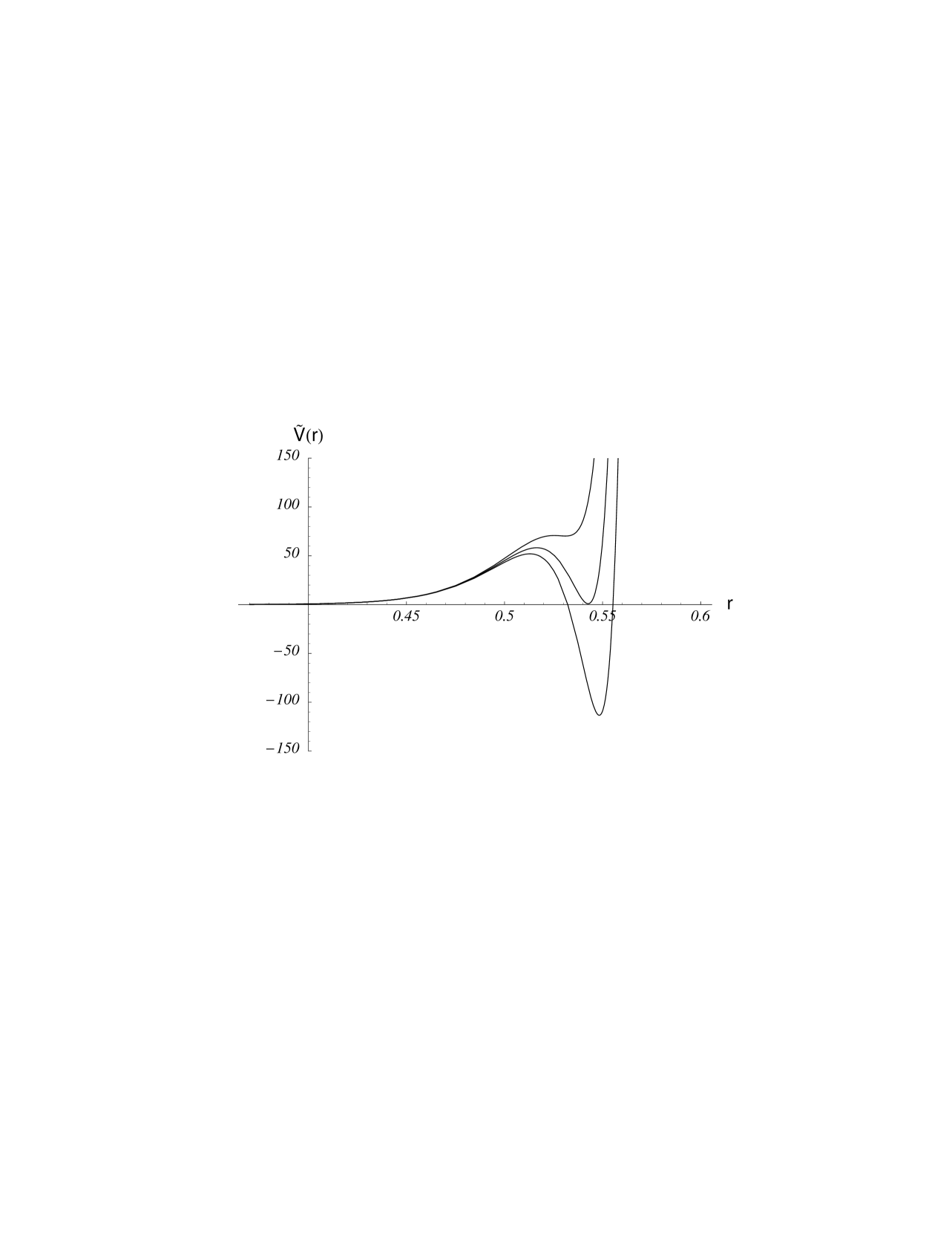
Figure 1: Potential along the flat ‘K’ direction, $\phi$, vs field values (parameterized by $r=1+\frac{6\alpha(M_{GUT})}{4\pi}\log\left(\frac{h_{t}\phi}{M_{GUT}}\right)$) for $m_{0}/M_{1/2}=$ 1.03, 1.05, 1.07.

We first borrow some results from later sections to get some idea of the shape of the potential along the $F$ and $D$ flat direction. Figure 1 shows

$$\tilde{V}=Vh_{b}^{2}/\mu^{2}M_{1/2}^{2}$$ (6)

in the K direction (with $j=3$) in the CMSSM for the three values of $m_{0}$ indicated. It is plotted in the approximation that we can neglect the bottom and tau Yukawa couplings and two-loop corrections in the running of parameters. (A full two-loop numerical running produces something similar.) We have taken $\mu=500\,{\rm GeV}$, $m_{b}(m_{t})=2.5\,{\rm GeV}$ and $\alpha_{3}(m_{t})=0.108$. The potential is taken at the quasi-fixed point so we don’t have to worry about the value of $A_{0}$ but is otherwise typical. As can be seen, a new minimum forms radiatively when $m_{0}/M_{1/2}\,\raisebox{-2.58334pt}{$\buildrel<\over{\sim}$}\,1.07$ and becomes global when $m_{0}/M_{1/2}\,\raisebox{-2.58334pt}{$\buildrel<\over{\sim}$}\,1.05$. The latter value corresponds to the traditional UFB bound (modulo the approximations we are making here). The minimum in the flat direction (which we shall denote by $\phi$) forms when $a\equiv a_{min}=8.5$ so that $\phi_{min}=few\times 10^{6}\,{\rm GeV}$. One fact which will prove extremely useful when deriving the bounds analytically later is that it is the first term in the potential (i.e. $m_{2}^{2}+m_{L}^{2}$) which dictates the form and position of the radiatively induced minimum. The depth of the minimum is therefore $\sim m_{W}^{2}\phi_{min}^{2}=a_{min}^{4}\mu^{2}m_{W}^{2}/h_{b}^{2}$.

Now consider the decay rate into the new minimum at finite temperature. In Ref.[5] it was argued that the traditional UFB bounds are not necessary because the decay rate into the UFB directions is generally far too small. The suppression occurs due to the presence of a large, temperature (T) dependent barrier between the false vacuum (where we are living if the UFB bound is violated) and the true charge and/or colour breaking one. This barrier is generically present due to the flat direction, $\phi$, giving masses to fields to which it couples. For $\phi\,\raisebox{-2.58334pt}{$\buildrel>\over{\sim}$}\,T$ the contribution to the temperature dependent effective potential from a field, $i$, is suppressed as $e^{-m_{i}(\phi)/T}$ (where $m_{i}$ is the mass it derives from coupling to the flat direction) and the potential is the same as that at zero temperature with a curvature of order $m_{W}^{2}$ coming from the soft supersymmetry breaking terms (c.f. Eqn.(3)). For $\phi\sim 0$ the contribution to the effective potential is ${\cal{O}}(-T^{4})$. The escape point of the critical bubble is therefore of order $\phi\sim T^{2}/m_{W}$. Since the barrier height is of order $T^{4}$ the decay rate is suppressed by a factor $e^{-S_{3}/T}$ where $S_{3}\sim T^{4}/m_{W}^{3}$, which is huge unless $T<m_{W}$. At zero temperature the quantum tunneling rate is only large enough for vacuum decay to have taken place within the lifetime of the universe for very low values of $m_{0}$ [5].

The estimates of Ref.[5] apply equally to the dangerous K and C directions we are considering here. Actually we can make a much more accurate estimate of the action for the finite temperature decay when $m_{\phi}\ll T\ll\phi_{min}$ as follows. The one-loop finite temperature contribution to the effective potential is

$$V_{T}(\phi)={T^{4}\over 2\pi^{2}}\sum_{i}\pm n_{i}\int_{0}^{\infty}dq\ q^{2}{\rm ln}\left[1\mp{\rm exp}\left(-\sqrt{q^{2}+m_{i}^{2}(\phi)/T^{2}}\right)\right],$$ (7)

where the upper sign is for bosons, the lower one for fermions, and the $n_{i}$ are the corresponding degrees of freedom. The masses $m_{i}$ are field dependent parameters which generally have a wide range of values and increase roughly linearly with distance along the flat direction. The potential to calculate the decay rate is normalised to zero at the origin,

$$\Delta V_{T}(\phi)=V_{T}(\phi)-V_{T}(0).$$ (8)

The integral has the well known limits when $m_{i}\ll T$ and $m_{i}\gg T$;

$$\Delta V_{T}(\phi)=\left\{\begin{array}[]{cc}{T^{2}\over 24}\sum\left[n_{B}\Delta m_{B}^{2}+{n_{F}\over 2}\Delta m_{F}^{2}\right]&\mbox{ ;}\\ \pi^{2}\bar{g}_{*}T^{4}/90&\mbox{ ;}\end{array}\right.\begin{array}[]{c}m_{i}(\phi)\ll T\\ m_{i}(\phi)\gg T\end{array}$$

where $\Delta m^{2}\equiv m^{2}(\phi)-m^{2}(0)$ and

$$\bar{g}_{*}=n_{B}+(7/8)n_{F}$$ (9)

counts the difference between the degrees of freedom of the heavy particles at that particular value of $\phi$ (i.e. those for which $m_{i}\gg T$) and at $\phi=0$. Particles which are strongly coupled to the flat direction cause a steep rise in the effective potential near the origin. The contribution near $\phi=0$ can also be expressed as $V(\phi)=(m_{T}^{2}-m_{\phi}^{2})\phi^{2}/2$ where $m_{\phi}^{2}\sim m_{W}^{2}$ is the (negative) zero temperature mass-squared of the $F$ and $D$-flat direction and

$$m_{T}^{2}={T^{2}\over 24}\sum\left[n_{B}\lambda_{B}^{2}+{n_{F}\over 2}\lambda_{F}^{2}\right]$$ (10)

in which $\lambda_{B,F}$ stands for the coupling of the field to the flat direction ($\sim g_{3}$, $g_{2}$ or $h_{t}$ in this case). (We take the mass-squared to be constant (and always negative) for this estimate.) The finite-temperature contribution to the effective potential of particles which couple to the flat direction can therefore be approximated by

$$V(\phi)=\frac{\kappa^{2}}{2}\phi^{2}T^{2}\Theta(\kappa T-\kappa^{\prime}\phi)+\left(\frac{\kappa^{\prime 2}}{2}T^{4}+\frac{m^{2}_{\phi}}{2}\left(\frac{\kappa^{2}}{\kappa^{\prime 2}}T^{2}-\phi^{2}\right)\right)\Theta(\kappa^{\prime}\phi-\kappa T),$$ (11)

where we have defined

$$\kappa^{2} = (m_{T}^{2}-m_{\phi}^{2})/T^{2}$$

$$\kappa^{\prime 2} = \pi^{2}\bar{g}_{*}/45.$$ (12)

The first term is the $\phi\ll T$ limit, the second term is the $\phi\gg T$ limit, and the last term is the zero temperature contribution which is still present when $\phi\gg T$. (The second $T^{2}$ term is just to match at $\kappa^{\prime}\phi=\kappa T$.) For the moment we are assuming that all the particles couple to $\phi$ equally and one should bear in mind that in the MSSM there are of course many different couplings. To get the decay rate we find the 3-dimensional euclidean action for a (spherically symmetric) critical bubble, $\phi(\rho)$ where $\rho$ is the radial coordinate. The bubble is a solution of the equation [8]

$$\frac{\partial^{2}\phi}{\partial\rho^{2}}+\frac{2}{\rho}\frac{\partial\phi}{\partial\rho}=\frac{\partial V}{\partial\phi},$$ (13)

with the boundary conditions

$$\phi(\infty) = 0$$

$$\left.\frac{\partial\phi}{\partial\rho}\right|_{0} = 0.$$ (14)

By matching $\phi$ and $\partial\phi/\partial\rho$ at $\kappa^{\prime}\phi=\kappa T$, we find the solution

$$\phi(\rho)=\left\{\begin{array}[]{cc}\frac{\kappa T}{\kappa^{\prime}}\frac{\hat{\rho}}{\rho}\frac{\sin\rho m_{\phi}}{\sin\hat{\rho}m_{\phi}}&\rho<\hat{\rho}\\ &\\ \frac{\kappa T}{\kappa^{\prime}}\frac{\hat{\rho}}{\rho}e^{(\hat{\rho}-\rho)\kappa T}&\rho>\hat{\rho}\end{array}\right.$$

where the radius of the bubble is given by

$$\hat{\rho}=\frac{1}{m}\left(\pi-\tan^{-1}(m_{\phi}/\kappa T)\right)\approx\pi/m_{\phi}$$ (15)

and the escape point by

$$\phi(0)=\frac{\hat{\rho}m_{\phi}\kappa T}{\kappa^{\prime}\sin(\hat{\rho}m_{\phi})}\approx\frac{\pi\kappa^{2}}{\kappa^{\prime}}\frac{T^{2}}{m_{\phi}},$$ (16)

where the approximations are for $\kappa T\gg m_{\phi}$. The three dimensional euclidean action is then given by

$$S_{3}/T = 4\pi\int\rho^{2}\mbox{d}\rho\left(\frac{1}{2}\left(\frac{\mbox{d}\phi}{\mbox{d}\rho}\right)^{2}+V(\phi)\right)$$ (17)

$$= \frac{2\pi^{4}\kappa^{\prime 2}}{3}\frac{T^{3}}{m_{\phi}^{3}}\left(1-\frac{1}{\pi}\tan^{-1}(m_{\phi}/\kappa T)\right)^{3}\left(1+\frac{\kappa^{4}}{\kappa^{\prime 4}}\left(\frac{m_{\phi}}{\kappa T}\right)^{2}\right)$$

$$\approx \frac{2\pi^{6}\bar{g}_{*}}{135}\frac{T^{3}}{m_{\phi}^{3}}.$$

This action is independent of the precise couplings to the flat direction because we assumed that the temperature is high enough for it to be dominated by the very large escape point. Hence the action is the same when there are many different couplings to the flat direction, $\lambda_{i}$, provided that they are all either strong enough for particle $i$ to freeze out well before the escape point or weak enough for it to not contribute appreciably to the effective potential. These two conditions can be written;

either $$\lambda_{i} \gg m_{\phi}/T$$

or $$\lambda_{i} \ll m_{\phi}/\phi_{min}.$$ (18)

The criterion for the vacuum to have decayed within the lifetime of the universe is (see for Ref. [5] for example)

$$S_{3}/T\,\raisebox{-2.58334pt}{$\buildrel<\over{\sim}$}\,200.$$ (19)

For $T\gg m_{\phi}$ the action is indeed much more than $~{}200T$ and becomes larger for higher temperatures, from which we conclude that the false vacuum is unlikely to have decayed within the lifetime of the universe. At $T\sim m_{\phi}$ we would need to take into account all the field directions in order to estimate the rate as well as the depth of the electroweak symmetry breaking minimum which we were able to neglect above. However from the above and Ref.[5] it seems unlikely that the false vacuum would decay within the lifetime of the universe even in this case.

Now consider decay from the new minimum to the origin. This would be relevant if either the new minimum were local (e.g. if $1.05M_{1/2}<m_{0}<1.07M_{1/2}$ in figure 1) or if it were global at zero temperature but lifted by finite temperature corrections (of order $T^{4}$ where $T\ll\phi_{min}$). The barrier height (in figure 1 for example) is governed by the first term in the zero temperature potential, and is therefore of order $a_{min}^{4}\mu^{2}m_{W}^{2}/h_{b}^{2}$, and its width is of order $\phi_{min}=a_{min}^{2}\mu/h_{b}$. The critical bubble is determined by Eq.(13) in which the RHS is of order $(a_{min}^{2}\mu/h_{b})m_{W}^{2}$. We can obtain an estimate of the action by scaling out the dependence on parameters using the dimensionless variables $\tilde{\phi}=\phi h_{b}/(a_{min}^{2}\mu)$ and $\tilde{\rho}=m_{W}\rho$. At finite temperature a critical bubble has a three dimensional euclidean action given by

$$S_{3}=4\pi\frac{a_{min}^{4}\mu^{2}}{h_{b}^{2}m_{W}}f$$ (20)

where $f$ is the integral,

$$f=\int_{0}^{\infty}\tilde{\rho}^{2}\mbox{d}\tilde{\rho}\left(\frac{1}{2}\left(\frac{\partial\tilde{\phi}}{\partial\tilde{\rho}}\right)^{2}+V\frac{h_{b}^{2}}{a_{min}^{4}\mu^{2}m_{W}^{2}}\right),$$ (21)

which we expect to be of order $1$. The decay rate is therefore only significant for large temperatures. Decay out of the false vacuum (for the potential of figure 1) within the lifetime of the universe would require,

$$200T\,\raisebox{-2.58334pt}{$\buildrel>\over{\sim}$}\,4\pi\frac{a_{min}^{4}\mu^{2}}{h_{b}^{2}m_{W}}\sim 5\times 10^{11}\,{\rm GeV}.$$ (22)

Of course our approximation breaks down long before this temperature is reached since, when $T\gg\phi_{min}\sim 10^{6}\,{\rm GeV}$, the finite temperature contributions to the effective potential (proportional to $\phi^{2}T^{2}$ for $T\gg\phi$) will in any case destabilise the local minimum. The quantum tunneling rate is also suppressed; for significant tunneling within the lifetime of the universe the $O(4)$ symmetric ‘bounce’ solution [9] should have an action $S_{4}\,\raisebox{-2.58334pt}{$\buildrel<\over{\sim}$}\,400$. We estimate

$$S_{4}=2\pi^{2}\frac{a_{min}^{2}\mu^{2}}{h_{b}^{2}m^{2}_{W}}f^{\prime}\gg 400$$ (23)

where the integral

$$f=\int_{0}^{\infty}\tilde{\rho}^{3}\mbox{d}\tilde{\rho}\left(\frac{1}{2}\left(\frac{\partial\tilde{\phi}}{\partial\tilde{\rho}}\right)^{2}+V\frac{h_{b}^{2}}{a_{min}^{4}\mu^{2}m_{W}^{2}}\right),$$ (24)

which is again expected to be $\sim 1$.

With these two pieces of information to hand, it is clear that the traditional UFB bound is irrelevant; it can never be either necessary or sufficient. It is not necessary because if the universe were trapped in a metastable minimum at the origin it would not have decayed within its lifetime. It is not sufficient because had the universe been trapped in a radiatively induced local minimum it would also not have been able to decay.

Finally, we can address one of the suggestions in Ref.[5] for driving the universe to a metastable vacuum at the origin. Some sort of dynamical mechanism is probably required if such a scenario is to avoid fine tuning. This mechanism could simply be a sufficiently high temperature, $T_{R}$, in the early universe. Each field, $i$, then contributes positive curvature to the potential for $\lambda_{i}\phi<T_{R}$. (Other proposed mechanisms depend on the additional soft supersymmetry breaking terms which can be generated during inflation [10].) However the destabilisation of the radiatively induced minimum can only be guaranteed if $T_{R}$ is greater than the zero-temperature position of the radiatively induced minimum, $\phi_{min}$. For the examples we are considering,

$$T_{R}\,\raisebox{-2.58334pt}{$\buildrel>\over{\sim}$}\,few\times 10^{6}\,{\rm GeV}.$$ (25)

However when, as we are assuming, supersymmetry is communicated gravitationally there is a bound on the reheat temperature coming from nucleosynthesis; if $T_{R}$ is too high, nucleosynthesis is disrupted by the creation and subsequent late decay of gravitinos [11]. This translates into the bound,

$$T_{R}\,\raisebox{-2.58334pt}{$\buildrel<\over{\sim}$}\,10^{9}\,{\rm GeV}.$$ (26)

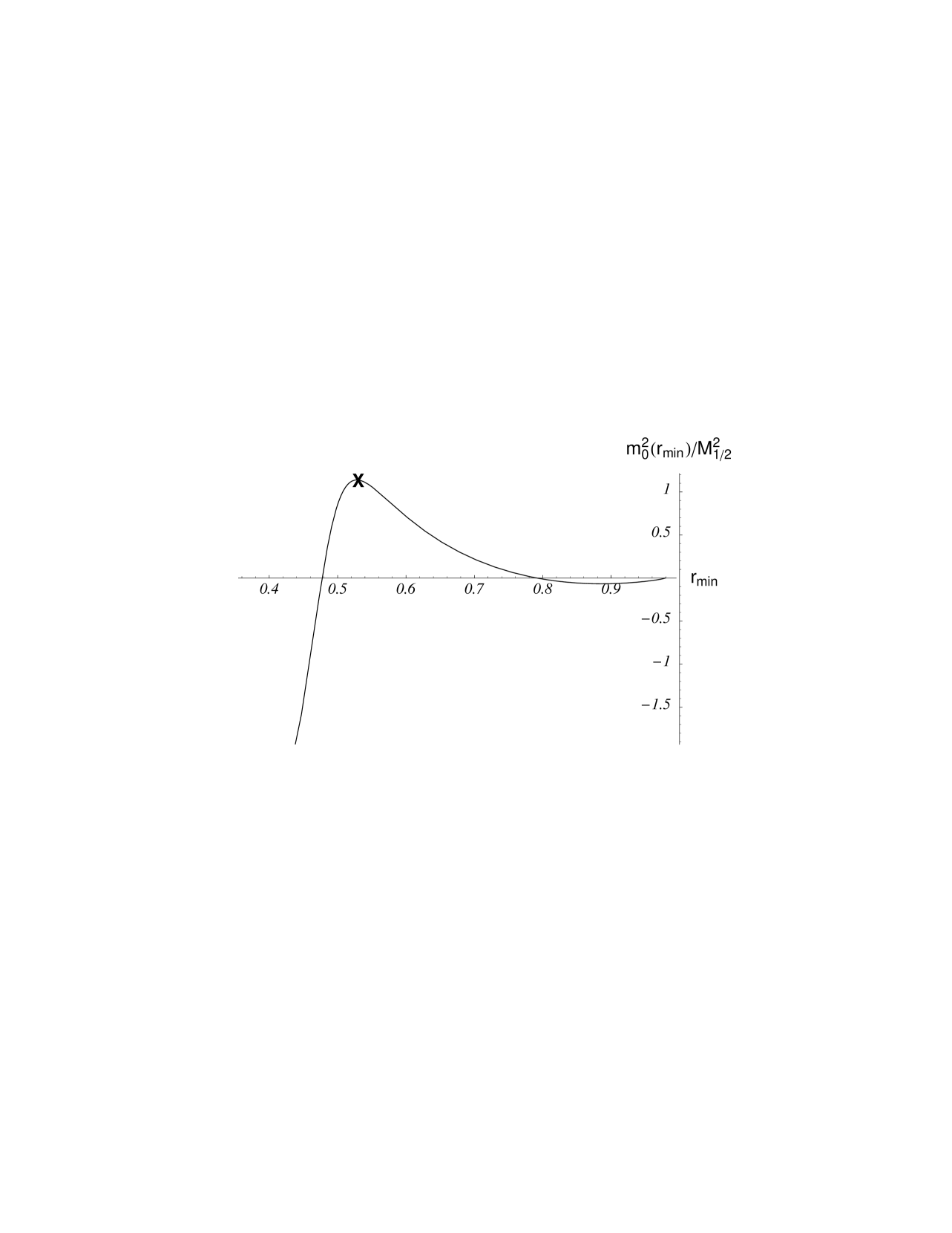
Figure 2: The value of $m_{0}^{2}$ corresponding to an extremum appearing at that field value (parameterized by $r$). Each value of $m_{0}$ generates one maximum (to the left of the cross) and one minimum (to the right). This example is at the quasi-fixed point.

Thus, when $m_{0}$ is close to the traditional UFB bound, the reheat temperature has to fall inside the window which is left. Moreover, this window closes when the traditional UFB bound is more strongly violated. Figure 2, which we will derive shortly, shows the position of extrema along direction K at the quasi-fixed point plotted against $m_{0}^{2}/M_{1/2}^{2}$ (with the same choice of parameters as in figure 1). To the right of the cross are only minima, to the left maxima. The cross corresponds to the point of inflexion in the $m_{0}=1.14M_{1/2}$ curve of figure 1. As $m_{0}^{2}$ decreases below the traditional UFB bound, the minimum deepens and $\phi_{min}$ grows rapidly. For low enough $m_{0}^{2}$, $T_{R}$ has to violate the bound in Eq.(26) if it is to destabilise the radiatively induced minimum. (For the quasi-fixed point example in figure 2, the window disappears when $m_{0}\,\raisebox{-2.58334pt}{$\buildrel<\over{\sim}$}\,0.7M_{1/2}$.) If the reheat temperature is far below $\phi_{min}$, then we have to ensure that the contribution to the effective potential from the more weakly coupled fields (proportional to $\lambda_{i}^{2}\phi^{2}T^{2}$ with $\lambda_{i}\ll 1$) is enough to drive $\phi$ to the origin, a complicated and model-dependent task.

To summarize, without a detailed knowledge of early cosmology, there is no well-defined criterion for excluding regions of parameter space based on the existence of deep minima along $F$ and $D$-flat directions, apart from at very small values of $m_{0}$ where quantum tunneling can take place within the lifetime of the universe. In the following sections therefore, as well as deriving the traditional UFB bound analytically, we shall focus on a sufficient condition which is better defined, namely that there are no minima other than the one at the origin. This condition ensures that the origin is reached from any initial $\phi$ even at zero temperature. The areas of parameter space which satisfy this condition are therefore allowed regardless of cosmology, and figure 1 suggests that, at least for the UFB directions we are considering here, they may not be very different from those allowed by the traditional UFB bound. At the quasi-fixed point for example, figure 1 gives the traditional bound to be $m_{0}\,\raisebox{-2.58334pt}{$\buildrel>\over{\sim}$}\,1.05M_{1/2}$ and the sufficient condition to be $m_{0}\,\raisebox{-2.58334pt}{$\buildrel>\over{\sim}$}\,1.07M_{1/2}$. Thus, in the one-loop approximation we are making (and possibly to two-loop order as well), the traditional UFB bound is indistinguishable from the sufficient condition.

3 Analytic derivation of ‘UFB’ bounds

In this section we develop an analytic treatment of both the traditional bound and sufficient condition coming from the K and C directions in the CMSSM at low $\tan\beta$. These are the two most restrictive constraints and were analysed numerically in Ref. [4]. We first summarize the one-loop RGE solutions, and then use them to obtain the bounds.

We shall obtain the bounds two ways in an order which may at first seem a little odd; we first present an accurate and straightforward but semi-graphical method, and then we present an entirely analytic method that requires some approximations. The reason for this ordering (it is after all more usual to first derive something approximately and then do it accurately) is that the second method is far more powerful, allowing us to produce bounds which are valid for all low $\tan\beta$. It also gives us more insight into how the bounds depend on the unknown parameters (such as $\mu$) and why they are numerically so close to each other. In fact we will conclude that (as anticipated in the previous section) two-loop accuracy is required to resolve the traditional bound and the sufficient condition.

To be able to do an analytic treatment, we will need to express the mass-squared parameters appearing in the potential as a function of scale (i.e. not as a numerical integral). This is possible if we work to one-loop and in the approximation that we can neglect couplings other than $\alpha_{2}$, $\alpha_{3}$ and $h_{t}$ in the running. We first give solutions for all the parameters in terms of the three quantities which are strongly attracted to quasi-fixed points in the minimal supersymmetric standard model (MSSM) (although other terms formally have quasi-fixed points too). The three parameters with quasi-fixed points are

$$R \equiv h_{t}^{2}/g_{3}^{2}$$

$$A_{t} \equiv A_{U_{33}}$$

$$3M^{2} \equiv m_{U_{33}}^{2}+m_{Q_{33}}^{2}+m_{2}^{2}.$$ (27)

When $h_{t}$ is high at the GUT or Planck scale (higher than 1 say), these three parameters are completely determined at the weak scale irrespective of the pattern of supersymmetry breaking at the GUT scale;

$$R^{QFP} = 0.87$$

$$A_{t}^{QFP} = -1.60M_{1/2}$$

$$(M^{2})^{QFP} = 1.83M_{1/2}^{2}.$$ (28)

Their values govern the running of the MSSM at low $\tan\beta$ [12]. (As pointed out in Refs.[13, 6] and references therein, various constrained versions of the MSSM lead to many more quasi-fixed points in addition to these three ubiquitous ones, and can lead to enhanced predictivity and reduced FCNCs at low $\tan\beta$.)

For completeness we present all the solutions for the flavour diagonal parameters here and for the moment leave in the $\alpha_{1}$ dependence; defining

$$\tilde{\alpha}_{i} = \frac{\alpha_{i}}{\alpha_{i}|_{0}}$$

$$\delta_{i}^{(n)} = \tilde{\alpha}^{n}_{i}-1$$

$$G = \frac{R}{R_{0}}\tilde{\alpha}_{3}^{-43/9}\tilde{\alpha}_{2}^{-3}\tilde{\alpha}_{1}^{-5/99}$$ (29)

where the $0$-subscript indicates values at the GUT scale, these are

$$A_{U_{ii}}-\frac{\mbox{\small 1}}{\mbox{\small 2}}A_{t} = M_{1/2}\left(-\frac{\mbox{\small 8}}{\mbox{\small 9}}\delta_{3}^{(1)}+\frac{\mbox{\small 3}}{\mbox{\small 2}}\delta_{2}^{(1)}+\frac{\mbox{\small 13}}{\mbox{\small 99}}\delta_{1}^{(1)}\right)+(A_{U_{ii}}-\frac{\mbox{\small 1}}{\mbox{\small 2}}A_{t})|_{0}$$

$$A_{b}-\frac{\mbox{\small 1}}{\mbox{\small 6}}A_{t} = M_{1/2}\left(-\frac{\mbox{\small 40}}{\mbox{\small 27}}\delta_{3}^{(1)}+\frac{\mbox{\small 5}}{\mbox{\small 2}}\delta_{2}^{(1)}+\frac{\mbox{\small 29}}{\mbox{\small 99}}\delta_{1}^{(1)}\right)+(A_{b}-\frac{\mbox{\small 1}}{\mbox{\small 6}}A_{t})|_{0}$$

$$A_{D_{ii}} = M_{1/2}\left(-\frac{\mbox{\small 16}}{\mbox{\small 9}}\delta_{3}^{(1)}+3\delta_{2}^{(1)}+\frac{\mbox{\small 7}}{\mbox{\small 99}}\delta_{1}^{(1)}\right)+(A_{D_{ii}})|_{0}$$

$$A_{E_{\alpha\alpha}} = M_{1/2}\left(3\delta_{2}^{(1)}+\frac{\mbox{\small 3}}{\mbox{\small 11}}\delta_{1}^{(1)}\right)+(A_{E_{\alpha\alpha}})|_{0}$$

$$B-\frac{\mbox{\small 1}}{\mbox{\small 2}}A_{t} = M_{1/2}\left(\frac{\mbox{\small 16}}{\mbox{\small 9}}\delta_{3}^{(1)}+\frac{\mbox{\small 3}}{\mbox{\small 2}}\delta_{2}^{(1)}+\frac{\mbox{\small 5}}{\mbox{\small 66}}\delta_{1}^{(1)}\right)+(B-\frac{\mbox{\small 1}}{\mbox{\small 2}}A_{t})|_{0}$$

$$m_{U_{33}}^{2}-M^{2} = M^{2}_{1/2}\left(\frac{\mbox{\small 8}}{\mbox{\small 27}}\delta_{3}^{(2)}+\delta_{2}^{(2)}-\frac{\mbox{\small 1}}{\mbox{\small 27}}\delta_{1}^{(2)}\right)+(m^{2}_{U_{33}}-M^{2})|_{0}$$

$$m_{Q_{33}}^{2}-\frac{\mbox{\small 1}}{\mbox{\small 2}}M^{2} = M^{2}_{1/2}\left(\frac{\mbox{\small 16}}{\mbox{\small 27}}\delta_{3}^{(2)}-\delta_{2}^{(2)}+\frac{\mbox{\small 5}}{\mbox{\small 297}}\delta_{1}^{(2)}\right)+(m^{2}_{Q_{33}}-\frac{\mbox{\small 1}}{\mbox{\small 2}}M^{2})|_{0}$$

$$m_{2}^{2}-\frac{\mbox{\small 3}}{\mbox{\small 2}}M^{2} = M^{2}_{1/2}\left(-\frac{\mbox{\small 8}}{\mbox{\small 9}}\delta_{3}^{(2)}+\frac{\mbox{\small 2}}{\mbox{\small 99}}\delta_{1}^{(2)}\right)+(m^{2}_{2}-\frac{\mbox{\small 3}}{\mbox{\small 2}}M^{2})|_{0}$$

$$m_{L_{\alpha\alpha}}^{2} = M^{2}_{1/2}\left(-\frac{\mbox{\small 3}}{\mbox{\small 2}}\delta_{2}^{(2)}-\frac{\mbox{\small 1}}{\mbox{\small 22}}\delta_{1}^{(2)}\right)+(m^{2}_{L_{\alpha\alpha}})|_{0}$$

$$m_{1}^{2} = M^{2}_{1/2}\left(-\frac{\mbox{\small 3}}{\mbox{\small 2}}\delta_{2}^{(2)}-\frac{\mbox{\small 1}}{\mbox{\small 22}}\delta_{1}^{(2)}\right)+(m^{2}_{1})|_{0}$$

$$m_{U_{ii}}^{2} = M^{2}_{1/2}\left(\frac{\mbox{\small 8}}{\mbox{\small 9}}\delta_{3}^{(2)}-\frac{\mbox{\small 8}}{\mbox{\small 99}}\delta_{1}^{(2)}\right)+(m^{2}_{U_{ii}})|_{0}$$

$$m_{Q_{ii}}^{2} = M^{2}_{1/2}\left(\frac{\mbox{\small 8}}{\mbox{\small 9}}\delta_{3}^{(2)}-\frac{\mbox{\small 3}}{\mbox{\small 2}}\delta_{2}^{(2)}-\frac{\mbox{\small 1}}{\mbox{\small 198}}\delta_{1}^{(2)}\right)+(m^{2}_{Q_{ii}})|_{0}$$

$$m_{D_{\alpha\alpha}}^{2} = M^{2}_{1/2}\left(\frac{\mbox{\small 8}}{\mbox{\small 9}}\delta_{3}^{(2)}-\frac{\mbox{\small 2}}{\mbox{\small 99}}\delta_{1}^{(2)}\right)+(m^{2}_{D_{\alpha\alpha}})|_{0}$$

$$\mu = \mu|_{0}G^{1/4}$$ (30)

where $i=1,2$ and $\alpha=1,2,3$.

The solutions of the remaining three parameters $R$, $A_{t}$ and $M^{2}$, can be expressed as functions of

$$r\equiv 1/\tilde{\alpha}_{3}=1+\frac{6\alpha_{0}}{4\pi}\log\frac{\Lambda}{M_{GUT}},$$ (31)

so that

$$\tilde{\alpha}_{2}=\frac{3}{4-r}\mbox{ ; }\tilde{\alpha}_{1}=\frac{5}{16-11r}.$$ (32)

Taking $\alpha_{3}(m_{t})=0.108$ means that $0.37<r<1$ with $r=1$ corresponding to the GUT scale. We shall use $r^{-1}$ and $\tilde{\alpha_{3}}$ intechangeably. If we define

$$\Pi(r) = \tilde{\alpha}_{3}^{16/9}\tilde{\alpha}_{2}^{-3}\tilde{\alpha}_{1}^{-13/99}$$

$$\hat{J} = \frac{1}{r\Pi(r)}\int^{1}_{r}\Pi(r^{\prime})\mbox{d}r^{\prime}$$ (33)

then, in terms of the GUT scale values ($R_{0}$, $A_{0}$, $m_{0}^{2}$) plus the functions

$$R^{QFP} = 1/2\hat{J}$$

$$\rho = \frac{R}{R^{QFP}}$$

$$\xi = \frac{1-r}{r\hat{J}}-1$$ (34)

we find

$$\frac{1}{R} = \frac{1}{R^{QFP}}+\frac{1}{R_{0}\Pi r}$$

$$A_{t} = (1-\rho)A_{0}+M_{1/2}\left(\rho\xi-(1-r)\left(\frac{16}{9}\tilde{\alpha}_{3}+\tilde{\alpha}_{2}+\frac{13}{45}\tilde{\alpha}_{1}\right)\right)$$

$$M^{2} = (1-\rho)m_{0}^{2}-\frac{1}{3}\rho K+\frac{2}{3}M_{1/2}^{2}(1-r)\gamma$$ (35)

where

$$K = (1-\rho)(\xi M_{1/2}-A_{0})^{2}-\xi^{2}M_{1/2}^{2}+M_{1/2}^{2}(1-r)(\xi+1)\left(\frac{16}{9}\tilde{\alpha}_{3}+\tilde{\alpha}_{2}+\frac{13}{45}\tilde{\alpha}_{1}\right)$$

$$\gamma = \frac{16}{9}\tilde{\alpha}_{3}(1+\tilde{\alpha}_{3}(1-r)/2)+\tilde{\alpha}_{2}(1-\tilde{\alpha}_{2}(1-r)/6)+\frac{13}{45}\tilde{\alpha}_{1}(1-11\tilde{\alpha}_{1}(1-r)/10).$$ (36)

There is only one integral to do, $\hat{J}$, which we must now approximate by dropping the $\alpha_{1}$ terms

$$\hat{J}r\Pi\approx-\frac{16479}{1540}+\frac{r^{-7/9}}{4620}(14080+36960r-1680r^{2}+77r^{3}).$$ (37)

This approximates the full integral to about 5% in the region of interest (i.e. where the minimum develops).

To make contact with the usual parameterisation of the CMSSM we can express the GUT scale parameter $R_{0}$ as a function of of the weak scale parameter $\tan\beta$ for which we need to insert the running top quark mass, $m_{t}(m_{t})=167\,{\rm GeV}$, and use

$$R=\frac{m_{t}^{2}}{4\pi\alpha_{3}v^{2}\sin^{2}\beta}$$ (38)

where $v=174.1\,{\rm GeV}$. Inserting the solution for $R$ gives

$$R_{0}^{-1} = \Pi r_{t}\frac{4\pi\alpha_{3}v^{2}}{m_{t}^{2}}\left(\sin^{2}\beta-\sin^{2}\beta^{QFP}\right)$$ (39)

$$= 6.34\left(\sin^{2}\beta-\sin^{2}\beta^{QFP}\right).$$

In this approximation $(\tan\beta)^{QFP}=1.89$. However the value we infer for $R_{0}$ is clearly highly dependent on its exact value and hence is sensitive to two-loop corrections. In this sense $R_{0}$ is a more natural parameter to use than $\tan\beta$; the latter is equivalent to a very peculiar weighting of the GUT scale parameter, so that mid-range values of $\tan\beta$ all correspond to roughly the same minimum value of $R_{0}$. As a nod to convention, however, we will present some of our results in terms of $\tan\beta$.

Now let us use these expressions to examine the potential of Eq.(3) in more detail for the case of the CMSSM in the $j=3$ direction. We first use a semi-graphical method to extract the traditional bound and sufficient condition.

The mass-squared parameters run with scale, and the appropriate scale, $\Lambda$, to evaluate them at is where the finite one-loop contributions (which we are neglecting) to the effective potential are small, $\Lambda\sim h_{t}\phi$ (assuming that the minimum occurs for $a\gg 1$ which we shall verify in a moment). This should correspond roughly to the largest mass if we were to diagonalise the mass matrices and evaluate the one-loop contribution completely. $a$ can then be expressed as a function of $r$,

$$a^{2}(r)=b(r)\exp(c(r-1))$$ (40)

where

$$b(r) = \frac{M_{GUT}h_{b}}{h_{t}\mu}=\frac{2.85\times 10^{12}}{h_{t}(r)/1.1}\left(\frac{M_{GUT}}{2\times 10^{16}\,{\rm GeV}}\right)\left(\frac{m_{b}(r)}{2.5\,{\rm GeV}}\right)\left(\frac{200\,{\rm GeV}}{\mu(r)}\right)$$

$$c = 4\pi/6\alpha_{3}|_{0}=52.4$$ (41)

where the central values are those we shall adopt for the scale $\Lambda=m_{t}$ or $r=r_{t}$. We can solve for $b(r)$ in the same manner as above, and find

$$b(r) = b|_{0}\left(\frac{R}{R_{0}}\right)^{-2/3}\tilde{\alpha}_{3}^{14/27}\tilde{\alpha}_{2}^{-1/2}\tilde{\alpha}_{1}^{-7/594}$$ (42)

$$\approx b(r_{t})\left(\frac{R(r)}{R(r_{t})}\right)^{-2/3}\left(\frac{\alpha_{3}(r)\alpha_{2}(r_{t})}{\alpha_{3}(r_{t})\alpha_{2}(r)}\right)^{1/2}$$

Denoting the position of the radiative minimum by $\phi_{min}$, the traditional bound is saturated by

$$\left.V\right|_{\phi_{min}}=\left.\frac{\partial V}{\partial\phi}\right|_{\phi_{min}}=0$$ (43)

and the sufficient condition is given by

$$\left.\frac{\partial V}{\partial\phi}\right|_{\phi_{min}}=\left.\frac{\partial^{2}V}{\partial\phi^{2}}\right|_{\phi_{min}}=0,$$ (44)

and so we can work with

$$\tilde{V}=Vh_{b}^{2}/\mu^{2}M_{1/2}^{2}$$ (45)

which depends only on $b(r)$. (This means that for the sufficient condition we are neglecting the running of $h_{t}$ which is relatively small in this region.) The potential becomes

$$\tilde{V}(r,m_{0}) = \frac{a^{2}(r)}{M_{1/2}^{2}}\left[a^{2}(r)(\frac{\mbox{\small 3}}{\mbox{\small 2}}M^{2}+\frac{\mbox{\small 1}}{\mbox{\small 2}}m_{0}^{2}-M_{1/2}^{2}(\frac{\mbox{\small 8}}{\mbox{\small 9}}\delta_{3}^{(2)}+\frac{\mbox{\small 3}}{\mbox{\small 2}}\delta_{2}^{(2)}+\frac{\mbox{\small 5}}{\mbox{\small 198}}\delta_{1}^{(2)}))\right.$$ (46)

$$+\left.\frac{\mbox{\small 1}}{\mbox{\small 2}}M^{2}+\frac{\mbox{\small 5}}{\mbox{\small 2}}m_{0}^{2}+M_{1/2}^{2}(\frac{\mbox{\small 40}}{\mbox{\small 27}}\delta_{3}^{(2)}-\frac{\mbox{\small 5}}{\mbox{\small 2}}\delta_{2}^{(2)}-\frac{\mbox{\small 29}}{\mbox{\small 594}}\delta_{1}^{(2)})\right]$$

Figure 1 shows $\tilde{V}$ for $m_{0}=1.03M_{1/2}$, $1.05M_{1/2}$, and $1.07M_{1/2}$, for the central values of parameters we used in Eqn.(3) and for the quasi-fixed point where $R_{0}^{-1}=0$ and where there is no dependence on $A_{0}$ in the mass-squareds. The minima of $V$ are at $\phi_{min}=few\times 10^{6}\,{\rm GeV}$. At the quasi-fixed point the traditional bound is saturated with a minimum corresponding to $a_{min}=a(0.5427)=8.5$, justifying our assumption of $a^{2}\gg 1$ in direction K.

As can be seen, for these values of $m_{0}$ the minimum is being rapidly lifted, with $m_{0}=1.05M_{1/2}$ saturating the traditional UFB bound. From this figure we have already anticipated one of our main conclusions; radiatively induced minima along UFB directions are lifted very quickly by changes in the parameters ($m_{0}$ in this case). This happens because the negative $a(r)^{4}$ term in the potential balances the positive $a(r)^{2}$ one when the traditional UFB bound is saturated, so that the height of the minimum is varying rapidly.

Ideally one would like to be able to locate the extrema for a given $m_{0}$, $R_{0}$ and $A_{0}$, see for what value of $m_{0}$ there exists a minimum away from the origin, and hence derive the traditional UFB bound. To make the problem tractable analytically we can use the fact that there is a one-to-two correspondence between $m_{0}$ and the location of the extrema, $r=r_{min}$. Consider again the K direction, with a minimum at $\phi_{min}=a_{min}^{2}\mu^{2}/h_{b}^{2}$ corresponding to

$$r_{min}=1+\frac{6\alpha(M_{GUT})}{4\pi}\log\left(\frac{a_{min}^{2}}{b}\right),$$ (47)

and denote the value of $m_{0}$ corresponding to an extremum at $r=r_{min}$ by $m_{0}(r_{min})$. Solving for $m^{2}_{0}(r_{min})$ is relatively simple since $V(r,m_{0})$ depends only linearly upon it;

$${m^{2}_{0}(r_{min})} = \frac{M_{1/2}^{2}}{d(a^{2}+\frac{\mbox{\small 5}}{\mbox{\small 2}})}\left[-(a^{2}+\frac{\mbox{\small 1}}{\mbox{\small 3}})R(r_{min})r_{min}^{-1}(3M^{2}+A_{t}^{2})-d(a^{2}+\frac{\mbox{\small 1}}{\mbox{\small 6}})M^{2}\right.$$ (48)

$$\mbox{\hskip 56.9055pt}+\frac{\mbox{\small 32}}{\mbox{\small 9}}\tilde{\alpha}^{3}_{3}+2(a^{2}+1)\tilde{\alpha}^{3}_{2}+\left(\frac{\mbox{\small 2}}{\mbox{\small 5}}a^{2}+\frac{\mbox{\small 14}}{\mbox{\small 15}}\right)\tilde{\alpha}^{3}_{1}$$

$$\mbox{\hskip 28.45274pt}\left.+d\left(\frac{\mbox{\small 16}}{\mbox{\small 9}}a^{2}-\frac{40}{27}\right)\delta^{(2)}_{3}+d\left(3a^{2}+\frac{\mbox{\small 5}}{\mbox{\small 2}}\right)\delta^{(2)}_{2}+d\left(\frac{\mbox{\small 5}}{\mbox{\small 99}}a^{2}+\frac{\mbox{\small 29}}{\mbox{\small 594}}\right)\delta^{(2)}_{1}\right]$$

where $d(r)$ encompasses the running of $a^{2}$;

$$d(r) = \frac{1}{a^{2}}\frac{da^{2}}{dr}=\frac{d\log b}{dr}+c$$ (49)

$$= \frac{1}{2}\tilde{\alpha}_{2}+\frac{1}{6}\tilde{\alpha}_{1}-\frac{4}{3r}R+c.$$

Eq.(48) is implicit in that, away from the fixed point, $M^{2}$ itself depends upon $m_{0}^{2}$. However, since the dependence is (by dimensions) also linear the full (but unwieldy) expression can easily be obtained from the above.

For a given value of $A_{0}$ and $R_{0}$ (or equivalently $A_{0}$ and $\tan\beta$) we can now find the sufficient condition from Eq.(48). First consider the quasi-fixed point. Figure 2 shows $m_{0}^{2}(r_{min})/M_{1/2}^{2}$ plotted against $r_{min}$. Values of $r_{min}$ to the left of the cross are maxima, to the right, minima of the potential for a given value of $m_{0}$. This function has a maximum when $m_{0}^{2}=1.14M_{1/2}^{2}$ so that the only minimum when $m_{0}>1.07M_{1/2}$ is at the origin, as we saw in figure 1. Close to the quasi-fixed point the sufficient condition can be approximated by expanding in $1/R_{0}$ and by noting that, from the analytic solutions, they can be expressed as

$$\frac{m_{0}^{2}}{M_{1/2}^{2}}>c_{0}+\left(c_{1}+c_{2}\frac{A_{0}}{M_{1/2}}+c_{3}\frac{A_{0}^{2}}{M_{1/2}^{2}}\right)/R_{0}+{\cal{O}}(1/R_{0}^{2}).$$ (50)

By matching at the quasi-fixed point and at $R_{0}=5$ and $A_{0}=(-1,~{}0,~{}1)$, we find that $c_{0..3}$= 1.14, -1.69, -0.63, 0.30 respectively. These numbers approximate the bound (in the one-loop approximation) to better than 5% for $R_{0}\,\raisebox{-2.58334pt}{$\buildrel>\over{\sim}$}\,4$ (corresponding to $h_{t}(M_{GUT})>1.4$) and $|A_{0}|\,\raisebox{-2.58334pt}{$\buildrel<\over{\sim}$}\,M_{1/2}$ and of course much better for larger $R_{0}$. We can also find an ‘absolute’ condition by completing the square in Eq.(50); values of $m_{0}$ which satisfy the sufficient condition in direction K must also satisfy

$$\frac{m_{0}^{2}}{M_{1/2}^{2}}>c_{0}+(c_{1}-c_{2}^{2}/4c_{3})/R_{0}=1.1-2.0/R_{0}.$$ (51)

If $m_{0}^{2}$ is below this bound a minimum is radiatively generated whatever the value of $A_{0}$.

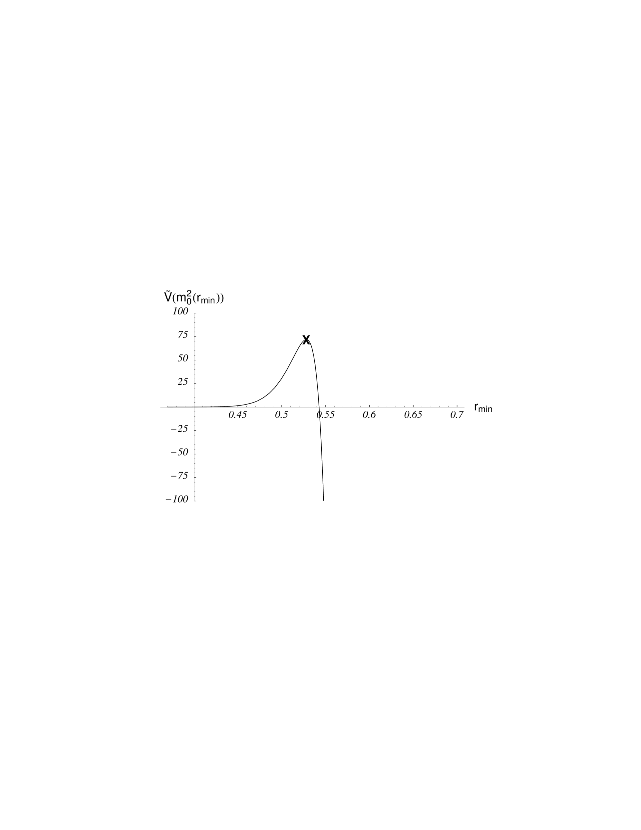
Figure 3: The height of the extrema vs their field value (parameterized by $r$). This example is at the quasi-fixed point and corresponds to substituting the $m^{2}_{0}$ values in figure 2 into the potential.

We can now find the traditional UFB bound graphically by plotting the height of the extrema, $V(r_{min},m_{0}(r_{min}))$, as shown in figure 3. At the quasi-fixed point, the minimum becomes negative at $r_{min}=0.5427$, giving the bound $m_{0}\,\raisebox{-2.58334pt}{$\buildrel>\over{\sim}$}\,m_{0}(0.5427)=1.05M_{1/2}$. Again by matching at the quasi-fixed point and at $R_{0}=5$ and $A_{0}=(-1,~{}0,~{}1)$, we find the coefficients $c_{0..3}$= 1.10, -1.67, -0.63, 0.30. Thus the sufficent condition is as expected virtually indistinguishable from the traditional bound.

Applying the same treatment to direction C at low $\tan\beta$ (which was studied numerically in Ref.[4]), we find $c_{0..3}$= 1.15, -1.54, -0.57, 0.26 for the traditional UFB bound and for the sufficient condition we find $c_{0..3}$= 1.17, -1.56, -0.57, 0.26. (For this direction the definition of $a^{2}$ the same, but with $b(r_{t})=1.9\times 10^{12}$ for $m_{\tau}(r_{t})=1.7\,{\rm GeV}$.) These bounds are in agreement with Ref.[4] given our neglect of two-loop contributions to the running of the gauge and Yukawa couplings. Ref.[4] finds $m_{0}\,\raisebox{-2.58334pt}{$\buildrel>\over{\sim}$}\,M_{1/2}$ at the quasi-fixed point (which should be compared with our result above of $m_{0}>1.05M_{1/2}$).

Finally let us consider the accuracy of the approximations we made. We saw that radiatively induced minima along UFB directions are lifted very quickly by changes in $m_{0}$. This means that the bounds are less sensitive to our lack of knowledge about the parameter $b$ and in fact depend on it only logarithmically as we shall see shortly. (In fact the error involved is of the same order as that we associate with neglecting the finite one-loop corrections.) We can also see that the bound increases with $b$ as we would expect since increasing $b$ increases the negative contribution to the potential from $m_{2}^{2}$. This is in accord with Ref.[4] where the effect of increasing the ‘unification’ scale to the Planck scale was examined. We also see that the bound increases with $m_{b}$ (which is why we chose $j=3$) and decreases with $\mu$. The variation of the bound with $A_{0}$ is quadratic becoming stronger at large $\tan\beta$ with a minimum close to $A_{0}=0$ at positive $A_{0}$.

Although the above method is accurate for a given choice of $A_{0}$ and $\tan\beta$ (given the other approximations we have made), it is cumbersome and in particular is not well suited to finding bounds at smaller values of $R_{0}$. In addition we would like to understand why the sufficient condition is numerically so close to the traditional bound. Because of this we now turn to a completely analytic derivation of the same bounds.

For this we can use the fact that the minimum appears at a scale where the first term in the potential is driven negative by $m_{2}^{2}$. So, considering direction K, if we define $A(r)=(m_{2}^{2}+m_{L_{i}}^{2})/M_{1/2}^{2}$ and $B(r)=(m_{L_{i}}^{2}+m_{d_{j}}^{2}+m_{Q_{j}}^{2})/M_{1/2}^{2}$, the minimum of the potential is at a scale close to the point which we shall call $r_{p}$ where $A$ becomes negative, $A(r_{p})=0$. We define two additional scales; $r_{d}\equiv$ the position of the minimum when the traditional UFB bound is saturated (i.e. when the minimum is degenerate with the origin), and $r_{c}\equiv$ the position of the point of inflexion when the sufficient condition is satisfied. We first determine these scales in terms of $r_{p}$ as follows. It is convenient to work with

$$\hat{V}=\frac{h_{t}^{2}}{M_{1/2}^{2}M_{GUT}^{2}}V=\left(e^{2c(r-1)}A+e^{c(r-1)}B/b\right),$$ (52)

(Note that instead of $M_{GUT}$ we could have used any scale, $\Lambda_{X}$, as long as $c=4\pi/6\alpha_{3}|_{\Lambda_{X}}$.) Since the scales $r_{p}$ will appear algebraically in the determination of the bounds we can sacrifice a little accuracy in their determination, and approximate the potential close to $r_{p}$ by developing $A(r)$;

$$\hat{V}(r)\approx(r-r_{p})\dot{A}(r_{p})e^{2c(r-1)}+e^{c(r-1)}B(r_{p})/b(r_{p}).$$ (53)

Because at this point $A$ is running much faster than $B$, $b$ and $h_{t}$, we are going to neglect the running of $B$, $b$ and $h_{t}$ close to $r_{p}$. For the bounds we will need

$$\dot{\hat{V}}(r) \approx (1+2c(r-r_{p}))\dot{A}e^{2c(r-1)}+e^{c(r-1)}cB/b$$

$$\ddot{\hat{V}}(r) \approx 4c(1+c(r-r_{p}))\dot{A}e^{2c(r-1)}+e^{c(r-1)}c^{2}B/b.$$ (54)

For the traditional UFB bound, ($\hat{V}(r_{d})=\dot{\hat{V}}(r_{d})=0$), we find

$$r_{p} = 1+\frac{1}{c}\ln\left(\frac{ecB}{\dot{A}b}\right)$$

$$r_{d} = r_{p}-1/c.$$ (55)

Likewise, for the sufficient condition, ($\ddot{\hat{V}}(r_{c})=\dot{\hat{V}}(r_{c})=0$), we find

$$r_{p} = 1+\frac{1}{c}\ln\left(\frac{e^{3/2}cB}{2\dot{A}b}\right)$$

$$r_{c} = r_{p}-3/2c.$$ (56)

Since $c$ is large (c.f. Eq.(3)) the minima are very close to $r_{p}$ (as was the case for the example shown in figure 1). The value of $r_{p}$ in each case is determined using the expression for $B$ above and for $\dot{A}$ which follows straightforwardly from the renormalisation group equations [14],

$$\dot{A}=\frac{R}{r}(3M^{2}+A_{t}^{2})-2\tilde{\alpha}_{2}^{3}-\frac{2}{5}\tilde{\alpha}_{1}^{3}.$$ (57)

A comparison of the expressions for $B$ and $\dot{A}$ together with $A(r_{p})=0$ gives

$$\dot{A}/B\approx R/r$$ (58)

to a good approximation independently of $m_{0}/M_{1/2}$. This allows for a sufficiently accurate determination of $r_{p}$ as the dependence on the parameters above is only logarithmic. For relatively large $R_{0}\,\raisebox{-2.58334pt}{$\buildrel>\over{\sim}$}\,1$ it is well approximated by using the quasi-fixed values of parameters in the logarithm

$$r_{p}=0.019\log(1.67+m_{0}^{2}/M_{1/2}^{2})+\left\{\begin{array}[]{cc}0.544&\mbox{traditional UFB}\\ 0.540&\mbox{sufficient }\end{array}\right.$$

The values of $r_{p}$ are those which must satisfy

$$A(r_{p})=0=\frac{\mbox{\small 3}}{\mbox{\small 2}}M^{2}+\frac{\mbox{\small 1}}{\mbox{\small 2}}m_{0}^{2}-M_{1/2}^{2}(\frac{\mbox{\small 8}}{\mbox{\small 9}}\delta_{3}^{(2)}+\frac{\mbox{\small 3}}{\mbox{\small 2}}\delta_{2}^{(2)}+\frac{\mbox{\small 5}}{\mbox{\small 198}}\delta_{1}^{(2)}),$$ (59)

and solving this gives the bounds on $m_{0}^{2}$ we are looking for. We find the approximate expression for the bound

$$\frac{m_{0}^{2}}{M_{1/2}^{2}}=\frac{4\rho_{p}-\rho_{p}^{2}-1.67+\rho_{p}(1-\rho_{p})\alpha}{4-3\rho_{p}}$$ (60)

where

$$\frac{1}{\rho_{p}} = 1+\left.\frac{R^{QFP}}{R_{0}\Pi r}\right|_{r_{p}}\approx 1+\frac{1}{3R_{0}}$$

$$\alpha \approx \frac{A_{0}^{2}}{M_{1/2}^{2}}-2\frac{A_{0}}{M_{1/2}}.$$ (61)

We again see from Eq.(60) that the bounds are always quadratic in $A_{0}$ (except for the very weak $A_{0}$ dependence in the determination of $r_{p}$). We also see that the bounds are much more restrictive for negative $A_{0}$ and have a minimum at $A\approx M_{1/2}$.

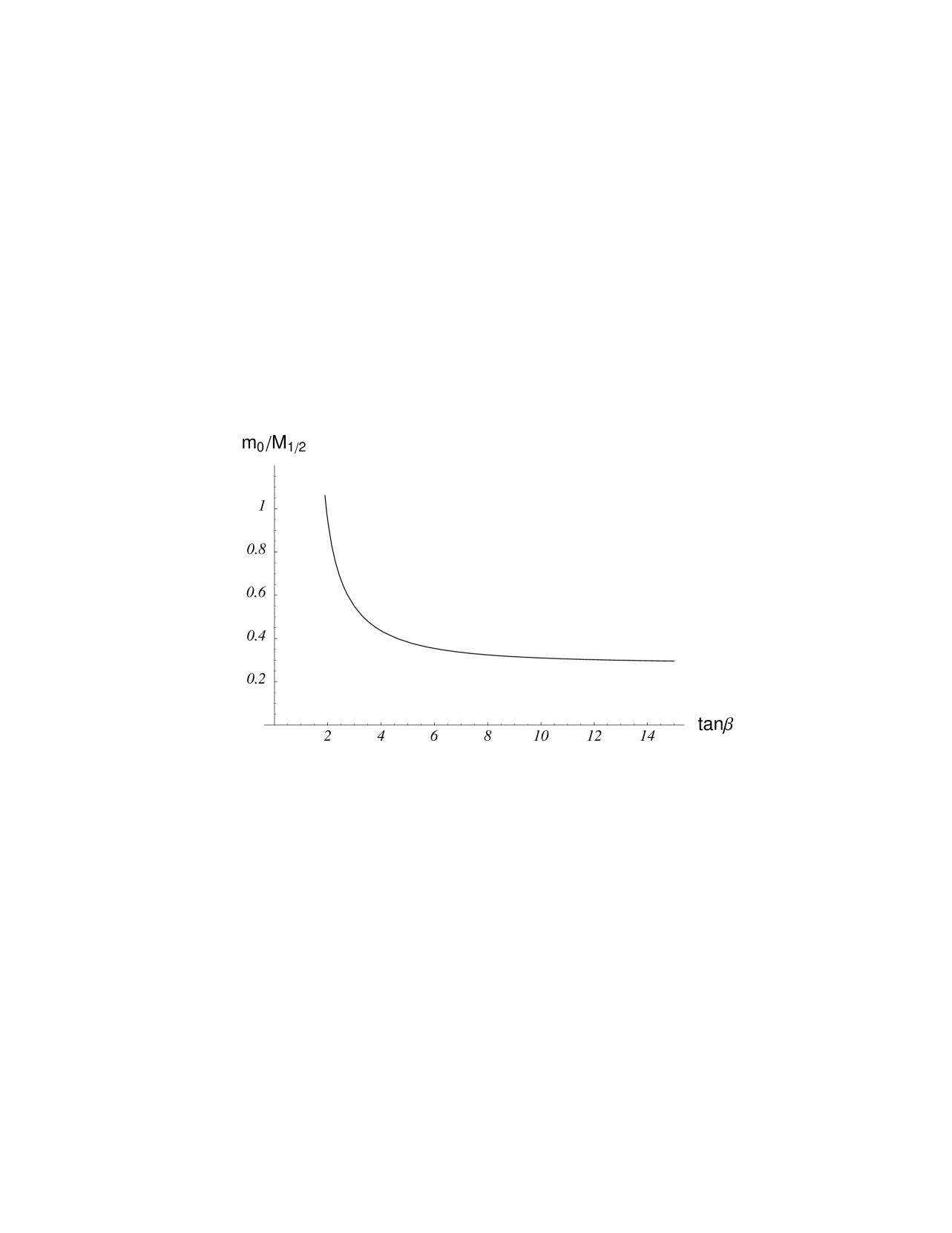
Figure 4: The sufficient condition for $\tan\beta<15$ and for any value of $A_{0}$. A minimum is formed radiatively when $m_{0}$ is below the line.

As an example of the usefulness of this method we show in figure 4 the ‘absolute’ bound on $m_{0}$ in this direction for all $\tan\beta<15$ where our RGE solutions are accurate to one-loop order. For values of $m_{0}$ below this bound there is a radiatively induced minimum whatever the value of $A_{0}$. Replacing $\rho_{p}$ in Eq.(60) with $\tan\beta$ gives a nice approximation to this diagram. (Since the diagram goes well away from the quasi-fixed point we found $r_{p}$ by solving the first equations of Eqs.(3,3) fully rather than using the large $R_{0}$ approximation above.) The plateau in figure 4 is a result of the mid-range values of $\tan\beta$ all corresponding to roughly the same value of $R_{0}$.

To compare this approximation with the previous method, we find the coefficients for the expansion near the quasi-fixed point of $c_{0..3}$= 1.13, -1.67, -0.63, 0.30 and $c_{0..3}$= 1.09, -1.65, -0.63, 0.30 for the sufficient condition and traditional UFB bounds respectively.

We can now see why the traditional UFB bound and the sufficient condition are so close. The separation between the scales $r_{d}$ and $r_{c}$ at which the minima form can only be of order ${\cal{O}}(1/c)$. When we solve for $A(r_{p})=0$ the values of $r_{p}$ differ by a factor $e^{1/2}/2=0.82$ appearing in the logarithm. Thus we would have to know $b$ and in particular $\mu$ to better than 18% (i.e. to two-loops) before we could distinguish the two bounds. On the other hand the parameter $r_{p}$ depends only logarithmically on $b$ but appears algebraically when we determine the bounds – hence the bounds on $m_{0}$ can only depend logarithmically on $b$.

4 Lifting flat directions with $R$-parity violation.

In this section we will see how much the flat directions can be lifted if we choose ‘baryon parity’ rather than $R$-parity to prevent proton decay [15].

As we stated in the introduction, violating $R$-parity can lessen UFB problems because there are less gauge invariants. The role of gauge invariants in flat directions was discussed in Ref.[7]. To clarify the role of the $R$-parity violating couplings let us briefly summarize that work. If we represent the scalar component of a generic superfield, $k$, as $z_{k}$, then the potential contains $D^{2}$ and $F^{2}$ terms where

$$D^{A}={\overline{z}}_{k}T^{A}_{kl}z_{l}$$ (62)

and $T^{A}$ are the matrices of the generators of the group. In addition, gauge invariance of any analytic function $I(z_{k})$ requires that

$$I_{k}T^{A}_{kl}z_{l}=0$$ (63)

where the subscript on the $I$ implies differentiation by $z_{k}$. Thus, there exists a $D$-flat direction corresponding to every

$$I_{k}|_{\langle z\rangle}=C{\langle{\overline{z}}_{k}\rangle},$$ (64)

where $C$ is a complex constant. The inverse, i.e. that every flat direction corresponds to an invariant satisfying Eq. (64), is a less trivial property. If the invariants in question do not appear in the superpotential, then the $F^{2}$ can often be made to cancel.

If we didn’t already know the UFB directions in the MSSM, then we could have used Eq.(64) to do it methodically (which is extremely useful for more complicated flat directions). For the K directions, the relevant invariants are

$$W = H_{1}(h_{D_{j}}Q_{j}D_{j}+\mu H_{2})$$

$$I = L_{i}(Q_{j}D_{j}+\mu^{\prime}H_{2})$$ (65)

where $W$ is a term in the superpotential while $I$ is not allowed if one assumes $R$-parity. The K direction in Eq. (1) is found as the solution of Eq.(64) for $I$ with the coefficient $\mu^{\prime}$ being chosen to cancel $F_{H_{1}}$, $\mu^{\prime}=-a^{2}\mu/h_{D_{j}}$. Similarly, the C direction can be constructed from the $R$-parity violating invariants

$$L_{i}L_{j}E_{j}\mbox{ ; }H_{2}L_{i}$$ (66)

with $i\neq j$.

Notice that the absence of a particular gauge invariant operator from the superpotential is not enough per se to ensure $F$-flatness unless no pair of superfields in the gauge invariant operator appear together in any term of the superpotential. For example $Q_{j}$ and $D_{j}$ both appear together in the Yukawa couplings of the MSSM and this is why we had to construct our flat direction by the conjunction of two invariants in order to cancel $F_{H_{1}}$. An example of a single gauge invariant which corresponds to an $F$ and $D$-flat direction is the other $R$-parity violating operator,

$$\epsilon UDD.$$ (67)

This flat direction (although it has been discussed at some length in the literature) is usually safe in models of gravitationally communicated supersymmetry breaking.

Baryon parity allows all of the invariant operators above corresponding to the K and C directions, and so can potentially lift all the flat directions we have been discussing. Since the K and C directions with $j=3$ result in comparable bounds on parameter space, we will assume that all the directions should be lifted in order to significantly change the conditions on parameters seen for example in figure 4. There are 5 flat directions in total, corresponding to $i=1,2,3$ in the K directions and $i=1,2$ in the C directions. In this section we will attempt to lift all five, whilst satisfying experimental constraints on $R$-parity violating operators.

We begin by adding to the superpotential the additional operators

$$W_{B}=\lambda_{ijk}L_{i}L_{j}E_{k}+\lambda^{\prime}_{ijk}L_{i}Q_{j}D_{k}.$$ (68)

We do not consider the $R$-parity violating bilinear operators, $\mu_{i}L_{i}H_{2}$, since the dimensionful coefficient $\mu_{i}$ must be much less than $m_{W}$ and so their contribution to the potential at large field values will be very small. Along the K and C directions the contributions to the potential from the $F^{2}$ terms are

$$V_{F-terms} = \sum_{m}\frac{a^{4}\mu^{4}}{h_{b}^{4}}\left(|\lambda^{\prime}_{m33}|^{2}+(1+a^{2})|\lambda^{\prime}_{im3}|^{2}+(1+a^{2})|\lambda^{\prime}_{i3m}|^{2}\right)$$

$$V_{F-terms} = \sum_{m}2\frac{a^{4}\mu^{4}}{h_{\tau}^{4}}\left(|\lambda_{m33}|^{2}+(1+a^{2})|\lambda_{im3}|^{2}+(1+a^{2})|\lambda_{i3m}|^{2}\right)$$ (69)

respectively. In addition one can expect contributions from new $R$-parity violating trilinear terms. Since the sign of the field (i.e. the sign of $a$) has not yet been determined, the potential will be minimised when they are negative;

$$V_{A-terms} \sim -|A_{\lambda^{\prime}}\lambda^{\prime}_{i33}\mu^{3}|\frac{|a|^{3}\sqrt{1+a^{2}}}{h_{b}^{3}}$$

$$V_{A-terms} \sim -|A_{\lambda}\lambda_{i33}\mu^{3}|\frac{|a|^{3}\sqrt{1+a^{2}}}{h_{\tau}^{3}}$$ (70)

respectively. The $F$-terms must overcome both these terms and the radiatively induced minimum at $\phi_{min}\approx a_{min}^{2}\mu/h_{b}$ if they are successfully to lift the flat direction.

We now discuss how big the new couplings have to be, generically, to lift the flat directions. Let us begin by making a rough estimate in which we say that the new $R$-parity violating $F$-terms have to ‘fill’ the radiatively induced minimum; i.e. we are neglecting the fact that the new terms change the position of the minimum. (We shall see shortly that this estimate is surprisingly good.) Since the depth of the minimum is $\sim a_{min}^{4}\mu^{2}m_{W}^{2}/h_{b}^{2}$, the $R$-parity violating couplings (generically denoted by $\lambda$ and $\lambda^{\prime}$) must satisfy

$$\lambda\,\raisebox{-2.58334pt}{$\buildrel>\over{\sim}$}\,\frac{h_{\tau}m_{W}}{a_{min}\mu}\approx 0.004\frac{m_{W}}{\mu}$$

$$\lambda^{\prime}\,\raisebox{-2.58334pt}{$\buildrel>\over{\sim}$}\,\frac{h_{b}m_{W}}{a_{min}\mu}\approx 0.004\frac{m_{W}}{\mu}.$$ (71)

The couplings $\lambda$ and $\lambda^{\prime}$ are understood to be evaluated at the scale of the minimum. If some of the flat directions are lifted by the $a^{4}$ terms in Eq.(4) then the $\lambda$ and $\lambda^{\prime}$ must be on the edge of experimental detection unless $\mu$ is very large [15]. We therefore concentrate on the $a^{6}$ terms and the condition above. Assuming that, as in canonical gravitationally communicated supersymmetry breaking, $A_{\lambda}\sim A_{\lambda^{\prime}}\sim m_{W}$ and that all of the $R$-parity violating couplings the same order of magnitude, the trilinear terms are dominated by the $F$-terms if Eq.(4) is satisified and $a_{min}\gg 1$.

We can refine our estimate substantially by adopting the approach of the last section. If $R$-parity violating terms are to make flat directions safe then we should, to be consistent, insist that there are no minima at all except the Standard-Model-like minimum for any value of parameters. Defining

$$\hat{\lambda}=\frac{\lambda\mu}{h_{\tau}M_{1/2}},$$ (72)

(and similar for $\lambda^{\prime}$) the form of the potential is now

$$\tilde{V}=Vh_{\tau}^{2}/\mu^{2}M_{1/2}^{2}=a^{4}A+a^{2}B+a^{6}\hat{\lambda}^{2},$$ (73)

where $a(r)$, $A(r)$ and $B(r)$ are as before. We now find the sufficient condition – i.e. a condition which ensures that the $R$-parity violation has destroyed all minima along the flat direction. The sufficient condition is then

$$\left.\frac{d^{2}{\tilde{V}}}{da^{2}}\right|_{r_{c}}=\left.\frac{d{\tilde{V}}}{da}\right|_{r_{c}}=0$$ (74)

where $A$ and $B$ are to be evaluated at the scale $r_{c}$ which we have yet to find. The determination of $r_{c}$ is simplified once we realise that all three terms are essential in the lifting of the minimum. The $a^{6}\hat{\lambda}^{2}$ term simply pushes the (extremely deep) minimum in the potential to low energy scales until it runs up against something positive – in this case the $a^{2}B$ term. Thus a suitable criterion for the determination of $r_{c}$ is simply that $a^{2}A(r_{c})+B(r_{c})=0$. Once we have $r_{c}$ we solve Eq.(74) treating $A$ and $B$ as constants and obtain the critical value of $\hat{\lambda}$. (The accuracy is extremely good because, in contrast to the determination of the UFB bounds, $A$ and $B$ are running very slowly at $r_{c}$). The value of $\hat{\lambda}$ is dependent on $m_{0}$, but if we want to add enough $R$-parity violation to remove the UFB problem entirely, we should do it at $m_{0}=0$ where the minimum is deepest. We therefore choose $m_{0}=0$ in our evaluation of $r_{c}$ and also (for simplicity) $A_{0}=0$. We find critical values

$$0.76>\hat{\lambda}_{crit}>0.50$$ (75)

with the upper value corresponding to $\tan\beta=1.8$ and the lower value to $\tan\beta=15$. (It drops to a plateau in $\tan\beta$ in much the same way as figure (4).) The revised estimate for the $R$-parity violation required to remove all UFB bounds is therefore

$$\lambda\,\raisebox{-2.58334pt}{$\buildrel>\over{\sim}$}\,\frac{0.76h_{\tau}M_{1/2}}{\mu}\approx 0.017\frac{M_{1/2}}{\mu}$$

$$\lambda^{\prime}\,\raisebox{-2.58334pt}{$\buildrel>\over{\sim}$}\,\frac{0.26h_{b}M_{1/2}}{\mu}\approx 0.009\frac{M_{1/2}}{\mu}.$$ (76)

Given that it is the $a^{6}$ terms which lift the flat directions, what set of $R$-parity violating couplings do we need? For the two C directions we can get away with having only one large coupling, $\lambda_{123}$. This coupling can satisfy Eq.(4) without violating current experimental bounds assuming that $\mu$ is not very much smaller than $M_{1/2}$; charged current universality requires that

$$\lambda_{123}<0.05\left(\frac{m_{\tilde{e}_{R}}}{100\,{\rm GeV}}\right).$$ (77)

For the K directions, we need at least three relatively large $\lambda^{\prime}$ couplings. In addition if we were, for example, to choose them to be $\lambda^{\prime}_{113}$, $\lambda^{\prime}_{213}$ and $\lambda^{\prime}_{313}$, then it is clear that we could just rotate the leptons into a basis where this is equivalent to just one coupling and we would still be left with two $F$-flat directions. We need to choose either $\lambda^{\prime}_{1a3},\lambda^{\prime}_{2b3},\lambda^{\prime}_{3c3}\neq 0$ or $\lambda^{\prime}_{13a},\lambda^{\prime}_{23b},\lambda^{\prime}_{33c}\neq 0$, where $a,b,c$ are all different (or any choice of three of these where the last two indices are all different). As an example, we choose $\lambda^{\prime}_{113},\lambda^{\prime}_{223},\lambda^{\prime}_{333}\neq 0$. The last two of these couplings are hardly constrained at all, and can easily satisfy experimental bounds [15] and Eq.(4) simultaneously. The first one however appears in quite restrictive bounds involving products of itself with one other $\lambda^{\prime}$ coupling. It is also constrained by charged current universality to be

$$\lambda^{\prime}_{113}<0.02\left(\frac{m_{\tilde{d}_{R}}}{100\,{\rm GeV}}\right).$$ (78)

Applying Eq.(4) to the product bounds in Ref.[15] results in new bounds for some of the other $R$-parity couplings. Assuming that the squark masses are $100\,{\rm GeV},$ for consistency with Ref.[15], they are

coupling  $\buildrel<\over{\sim}$	‘UFB’ limit $\times(\mu/M_{1/2})$	experimental limit
$\lambda^{\prime}_{111}$	0.0008	0.00035
$\lambda^{\prime}_{112}$	0.04	0.02
$\lambda^{\prime}_{121}$	0.03	0.035
$\lambda^{\prime}_{122}$	0.04	0.02
$\lambda^{\prime}_{131}$	$9.0\times 10^{-6}$	0.035
$\lambda^{\prime}_{132}$	0.17	0.33
$\lambda^{\prime}_{213}$	$6.0\times 10^{-6}$	0.09

When $\mu\approx M_{1/2}$ we see that most of the new bounds are comparable to the current experimental ones. The bounds on $\lambda^{\prime}_{132}$ and $\lambda^{\prime}_{121}$ are actually more restrictive and those on $\lambda^{\prime}_{131}$ and $\lambda^{\prime}_{213}$ much more restrictive.

To summarize, in minimal supersymmetry with constrained (degenerate) supersymmetry breaking, the addition of $R$-parity violation just below the current experimental bounds (c.f. Eq.(4)) is enough to lift dangerous flat directions and destroy local minima. For values of $\tan\beta$ which are away well from the quasi-fixed point the magnitude of the $R$-parity violating couplings required to do this drops rapidly by a factor of $\sim 2$.

5 Conclusions

Using approximate analytic solutions to the RGEs of the MSSM, we have examined the formation of minima in $F$ and $D$ flat directions. We have given arguments which suggest that the traditional UFB bounds are not meaningful since, even if a radiatively induced minimum is not global, the decay rate back to the physical vacuum is very small. We have rederived the traditional UFB bounds analytically, and shown that they are numerically very close to satisfying a more meaningful sufficient condition – that there be no radiatively induced minima along the flat direction at all. The sufficient condition was derived for all $\tan\beta<15$.

In the literature the question of dangerous flat direction is usually tackled by either making an implicit or at least not very detailed appeal to cosmology, or by completely excluding regions of parameter space where the physical vacuum is metastable – a condition which, as we have seen, is probably not even relevant. The unbiased approach we have been advocating is to locate in the parameter space regions where some (unknown) cosmological input is needed to save the model. The ‘traditional’ UFB bound does not do this since it is still possible to get caught in a charge and colour breaking minimum even if it not the global one (and hence satisfies the ‘traditional’ UFB bound). The sufficient condition we gave is only slightly more restrictive than the ‘traditional’ bound but is in our opinion the only possible relevant condition and is very different in spirit.

We also examined the effect of $R$-parity violation, and found that a small amount of $R$-parity violation (consistent with but just below current experimental limits) is able to lift the most dangerous flat directions and remove radiatively induced minima. In this way $R$-parity removes the metastability problems which plague the MSSM, and rescues some models which could be worth saving. One example is the MSSM at the quasi-fixed point which has much less dependence on initial parameters (as we have seen) and hence is more predictive [13, 6]. This model is likely to be severely constrained by a combination of UFB bounds and higgs bounds coming from LEP2 [13, 16]. A second example is the dilaton breaking scenario which has degenaracy in the supersymetry breaking terms (at tree level) and hence naturally suppressed flavour changing neutral currents. This model was excluded because of UFB bounds in Ref.[17].

6 Acknowledgements

We would like to thank Ben Allanach and Sacha Davidson for discussions and for a critical reading of the manuscript and also Toby Falk for additional comments.

References

- [1] J.-M. Frère, D.R.T. Jones and S. Raby, Nucl. Phys. B222 (1983) 11; M. Claudson, L. Hall and I. Hinchcliffe, Nucl. Phys. B228 (1983) 501; H.-P. Nilles, M. Srednicki and D. Wyler, Phys. Lett. B120 (1983) 346; J-P. Derendinger and C. A. Savoy, Nucl. Phys. B237 (1984) 307; P. Langacker and N. Polonsky, Phys. Rev. D50 (1994) 2199; A. Kusenko, P. Langacker and G. Segre, Phys. Rev. D54 (1996) 5824; H. Baer, M. Bhrlik and D. Castano, Phys. Rev. D54 (1996) 6944
- [2] H. Komatsu, Phys. Lett. B215 (1988) 323.
- [3] J.A. Casas and S. Dimopoulos, Phys. Lett. B387 (1996) 107; J.A. Casas, hep-ph/9707475 ; J.A. Casas, A. Lleyda and C. Munoz, Nucl. Phys. B471 (1996) 3.
- [4] J. A. Casas, A. Lleyda and C. Munoz, Phys. Lett. B389 (1996) 305
- [5] T. Falk, K. A. Olive, L. Roszkowski and M. Srednicki, Phys. Lett. B367 (1996) 183; A. Riotto and E. Roulet, Phys. Lett. B377 (1996) 60; A. Strumia, Nucl. Phys. B482 (1996) 24; T. Falk, K. A. Olive, L. Roszkowski, A. Singh and M. Srednicki, Phys. Lett. B396 (1997) 50
- [6] S.A. Abel and B.C. Allanach, Phys. Lett. B415 (1997) 371.
- [7] F. Buccella, J-P. Derendinger, C. A. Savoy and S. Ferrara, Phys. Lett. B115 (1982) 375; R. Gatto and G. Sartori, Phys. Lett. B157 (1985) 389; M. A. Luty and W. Taylor, Phys. Rev. D53 (1996) 3399; T. Ghergetta, C. Kolda, S. P. Martin, Nucl. Phys. B468 (1996) 37.
- [8] A. Linde, phys. Lett. B70 (1977) 206; 100B (1981) 37; A. Guth and E. Weinberg, Phys. Rev. D23 (1981) 876.
- [9] S. Coleman, Phys. Rev. D15 (1977) 2929; S. Coleman and C. Callan, Phys. Rev. D16 (1977) 1762.
- [10] M. Dine, W. Fischler and D. Nemeschansky, Phys. Lett. B136 (1984) 169; O. Bertolami and G. G. Ross, Phys. Lett. B183 (1987) 163; M. Gaillard, H. Murayama and K. A. Olive, Phys. Lett. B355 (1995) 71; G. Dvali, Phys. Lett. B355 (1995) 78; M. Dine, L. Randall and S. Thomas, Phys. Rev. Lett 75 (1995) 398; Nucl. Phys. B458 (1996) 291.
- [11] J. E. Ellis et al, Nucl. Phys. B373 (1992) 118; S. Sarkar, Rept. Prog. Phys. 59 (1996) 1493.
- [12] C. T. Hill, Phys. Rev. D24 (1981) 691; C. T. Hill, C. N. Leung and S. Rao, Nucl. Phys. B262 (1985) 517
- [13] V. Barger, M.S. Berger, P. Ohmann and R. J. N. Phillips, Phys. Lett. B314 (1993) 351; V. Barger, M.S. Berger and P. Ohmann Phys. Rev. D49 (1994) 4908; M. Carena, M. Olechowski, S. Pokorski and C. E. M. Wagner, Nucl. Phys. B419 (1994) 213; 426 (1994) 269; M. Carena and C. E. M. Wagner, Nucl. Phys. B452 (1995) 45; M. Lanzagorta and G.G. Ross, Phys. Lett. B349 (1995) 31; M. Lanzagorta and G.G. Ross, Phys. Lett. B364 (1995) 163.
- [14] K. Inoue, A. Kakuto, H. Komatsu and S. Kakeshita, Prog. Theor. Phys. 68 (1982) 927; Errata ibid. 70 (1983) 330.
- [15] H. K. Dreiner, hep-ph/9707435 ; G. Bhattacharyya and A. Raychaudhuri, hep-ph/9712245 ; G. Bhattacharyya, hep-ph/9709395
- [16] J. A. Casas, J. R. Espinosa and H. E. Haber, hep-ph/9801365 ; S. A. Abel and B. C. Allanach, hep-ph/9803476
- [17] J. A. Casas, A. Lleyda and C. Munoz, Phys. Lett. B380 (1996) 59