Abstract

Relying on the Luttinger-Ward theorem we derive a thermodynamically selfconsistent and scale independent approximation of the thermodynamic potential for the scalar $\phi^{4}$ theory in the tadpole approximation. The resulting thermodynamic potential as a function of the temperature is similar to the one of the recently proposed screened perturbation theory.

The usual perturbative evaluation of the QCD thermodynamic potential $\Omega(T)$ up to fifth order in the coupling constant $g$ [1] encounters the problem that the contributions $\propto g^{2}$ to $g^{5}$ alternate in sign and increase in magnitude and do not seem to approach a limiting value in the strong coupling regime. Therefore the hope has been formulated that a suitably reorganized perturbation theory can improve the calculation of $\Omega$. This problem has been attacked in refs. [2, 3]. For instance, in ref. [2] a screened loop expansion is employed which accounts for the screening in thermal propagators. Such an improvement of the convergence properties in analytical calculations of $\Omega$ is urgently necessary since recent lattice QCD calculations [4] have delivered accurate numerical results which now should be understood on a quantitative level in the physically relevant region, say up to temperatures of $5\,T_{c}$, where significant deviations from the asymptotic limit of $\Omega\propto T^{4}$ are still clearly seen. Near the confinement temperature $T_{c}$ these deviations are, of course, very large. One can describe such a behavior on the basis of effective theories with parameters adjusted to the lattice results (see [5, 6] for recent attempts and references quoted therein), but most ansätze are hampered by their ad hoc character or vague contact to QCD as the fundamental microscopic gauge field theory.

Since QCD has a quite complicated analytical structure, one should start to develop a systematic approach for simpler model field theories. Here we consider the scalar massless $\phi^{4}$ theory with the Lagrangian ${\cal L}=\frac{1}{2}(\partial_{\mu}\phi)(\partial^{\mu}\phi)-\frac{g^{2}}{4!}\phi^{4}$. For such a model the perturbative expansion of $\Omega$ is also performed up to fifth order [7], and it shows similar bad convergence properties as QCD at not too small coupling strength $g$. We are going to derive from the Luttinger-Ward theorem an approximation of $\Omega(T)$. The approach of Luttinger and Ward is known to be rather general and allows for selfconsistent approximations respecting the symmetries and conservation laws of the underlying full theory.

The Luttinger-Ward theorem can be formulated for the scalar theory as

$$\Omega = \frac{1}{2}TV\sum\int\;\{\ln(-\Delta^{-1})+\Delta\Pi\}+\Omega^{\prime},$$ (1)

$$\Omega^{\prime} = -\sum_{n}\frac{1}{4n}TV\sum\int\;\Delta\Pi^{s}_{(n)},$$ (2)

where $\Delta$ denotes the exact propagator and $\Pi$ the exact selfenergy; $\Pi^{s}_{(n)}$ stands for the contribution of the skeleton diagrams of $n$th order to the selfenergy (these are two-particle irreducible diagrams); $V$ is the volume of the system, and $\small{\vspace*{-3mm}\Sigma}\!\!\!\!\!\int$ is explained below. $\Omega$ has the property of stationarity [8], i.e.,

$$\frac{\delta\Omega}{\delta\Delta}=0,$$ (3)

which ensures the selfconsistent relation between $\Omega$, $\Delta$ and $\Pi$. Originally the relations (1, 2) have been derived for Fermi systems [9], later it has been extended to Bose systems [10]. For details of the derivation of the formulation (1, 2) we refer the interested reader to [11, 12].

Here we use eqs. (1, 2) to derive a consistent approximation of $\Omega$. Our starting point is the restriction to the tadpole contribution to the selfenergy. This implies that we take into account only the first term in the functional $\Omega^{\prime}$, i.e.,

$$\Omega^{\prime}_{(1)}=-\frac{1}{4}TV\sum\int\;\Delta_{(1)}\,\Pi^{s}_{(1)}=-3\put(0.0,3.0){\leavevmode\hbox{ \begin{picture}(0.0,0.0)\put(5.0,0.0){\circle{6.0}} \put(5.0,0.0){\circle{5.0}} \put(10.5,0.0){\circle{6.0}} \put(10.5,0.0){\circle{5.0}} \end{picture} }}$$ (4)

($\Delta_{(1)}$ and double lines in the diagrammatic representation denote the full propagator in the considered approximation). The corresponding selfenergy is due to eq. (3)

$$\Pi^{s}_{(1)}=12\left(\frac{-g^{2}}{4!}\right)T\sum\int\;\Delta_{(1)}=12\put(0.0,3.0){\leavevmode\hbox{ \begin{picture}(0.0,0.0)\put(5.0,0.0){\circle{6.0}} \put(5.0,0.0){\circle{5.0}} \put(0.0,-3.0){\line(1,0){10.0}} \end{picture} }}\hskip 28.45274pt\hskip 8.53581pt.$$ (5)

In the tadpole approximation the selfenergy is momentum independent and real. Therefore, in this approximation the corresponding resummed propagator looks like the free propagator modified by a term which resembles a mass term, i.e., $\Delta^{-1}\to\Delta^{-1}_{(1)}=\Delta^{-1}_{(0)}-\Pi_{(1)}^{s}$, and $\Pi_{(1)}^{s}$ is equivalent to the 1-loop selfenergy.

Since after performing the Matsubara sum the integrals over loop momenta are ultraviolet divergent one has to regularize. We employ the $\overline{\mbox{MS}}$ scheme in $4-2\epsilon$ dimensions, where

$$\sum\int\;=\left(\frac{e^{\gamma}\bar{\mu}^{2}}{4\pi}\right)^{\epsilon}\sum_{p_{0}}\int\frac{d^{3-2\epsilon}p}{(2\pi)^{3-2\epsilon}};$$ (6)

$\bar{\mu}$ is the renormalization scale, and $\gamma\approx 0.577$ is Euler’s number. An explicit calculation of eq. (5) yields

$$\Pi^{s}_{(1)} = 12\left(-\frac{g^{2}}{4!}\right)\left\{\frac{\Pi^{s}_{(1)}}{(4\pi)^{2}}\left[\frac{1}{\epsilon}+\ln\frac{\bar{\mu}^{2}}{T^{2}}-\ln\frac{\Pi^{s}_{(1)}}{T^{2}}+1\right]\right.$$ (7)

$$-\left.\frac{1}{2\pi^{2}}\int_{0}^{\infty}dp\,\frac{p^{2}}{\sqrt{p^{2}+\Pi^{s}_{(1)}}}\,\frac{1}{\exp\left\{\frac{\sqrt{p^{2}+\Pi^{s}_{(1)}}}{T}\right\}-1}+{\cal O}(\epsilon)\right\}$$

which is an implicit equation for $\Pi^{s}_{(1)}$. The first term $\propto\epsilon^{-1}$ corresponds to the divergent vacuum part in the usual vacuum selfenergy of the massive scalar theory. Since now $\Pi^{s}_{(1)}$ is temperature dependent, also this term is temperature dependent. Therefore, it cannot be cancelled by vacuum counter terms. It can be shown, however, that this term as well as the scale dependent term $\propto\ln(\bar{\mu}^{2}/T^{2})$ are cancelled by higher loop contributions. This can be seen explicitly when considering all contributions $\propto g^{4}T^{2}(\frac{1}{\epsilon}+\ln\frac{\bar{\mu}^{2}}{T^{2}})$ to the exact selfenergy. In our case the relevant contributions come from the above tadpole, $12\put(0.0,3.0){\leavevmode\hbox{ \begin{picture}(0.0,0.0)\put(5.0,0.0){\circle{6.0}} \put(5.0,0.0){\circle{5.0}} \put(0.0,-3.0){\line(1,0){10.0}} \end{picture} }}\hskip 34.1433pt\to 12\left(-\frac{g^{2}}{4!}\right)\frac{\Pi^{s}_{(1)}}{(4\pi)^{2}}(\frac{1}{\epsilon}+\ln\frac{\bar{\mu}^{2}}{T^{2}})$, the rising sun diagram, $96\put(0.0,3.0){\leavevmode\hbox{ \begin{picture}(0.0,0.0)\put(5.0,0.0){\circle{6.0}} \put(5.0,0.0){\circle{5.0}} \put(0.0,-0.1){\line(1,0){10.0}} \put(2.5,0.2){\line(1,0){5.0}} \end{picture} }}\hskip 34.1433pt\to-96\left(-\frac{g^{2}}{4!}\right)^{2}\frac{T^{2}}{(4\pi)^{2}}\frac{1}{4}(\frac{1}{\epsilon}+\ln\frac{\bar{\mu}^{2}}{T^{2}})$, and the vertex correction in the tadpole, $12\put(0.0,3.0){\leavevmode\hbox{ \begin{picture}(0.0,0.0)\put(5.0,0.0){\circle{6.0}} \put(5.0,0.0){\circle{5.0}} \put(0.0,-3.0){\line(1,0){10.0}} \put(5.0,-2.75){\circle*{2.0}} \end{picture} }}\hskip 34.1433pt\to-12\left(-\frac{g^{2}}{4!}\right)\frac{3g^{2}}{(4\pi)^{2}}\frac{T^{2}}{12}\frac{1}{2}(\frac{1}{\epsilon}+\ln\frac{\bar{\mu}^{2}}{T^{2}})$, which indeed cancel since in leading order $\Pi^{s}_{(1)}\to g^{2}T^{2}/4!$. The regularized part of eq. (7) thus allows the identification $\Pi^{s}_{(1)}\to m^{2}$ and reads at $\epsilon\to 0$ like a gap equation

$$m^{2}=\frac{g^{2}}{2}\left\{\frac{1}{2\pi^{2}}\int_{0}^{\infty}dp\,\frac{p^{2}}{\sqrt{p^{2}+m^{2}}}\frac{1}{\exp\left\{\frac{\sqrt{p^{2}+m^{2}}}{T}\right\}-1}+\frac{m^{2}}{(4\pi)^{2}}\left[\ln\frac{m^{2}}{T^{2}}-1\right]\right\},$$ (8)

which determines $m(T)$. Therefore, in our approach the gap equation is inherent, while in ref. [2] it is taken as an external information. With the definition $\Delta_{m^{2}}^{-1}=\Delta_{0}^{-1}-m^{2}$ our approximation of the thermodynamic potential is determined by

$$\Omega_{(1)} = \frac{1}{2}TV\sum\int\;\left\{\ln(-\Delta^{-1}_{m^{2}})+\frac{1}{2}m^{2}\Delta_{m^{2}}\right\}$$ (10)

$$= \frac{TV}{2\pi^{2}}\int_{0}^{\infty}dp\,p^{2}\ln\left(1-\exp\left\{-\frac{\sqrt{p^{2}+m^{2}}}{T}\right\}\right)$$

$$-\frac{m^{2}V}{8\pi^{2}}\int_{0}^{\infty}dp\,p^{2}\frac{1}{\sqrt{p^{2}+m^{2}}}\left[\exp\left\{\frac{\sqrt{p^{2}+m^{2}}}{T}\right\}-1\right]^{-1}-\frac{m^{4}}{128\,\pi^{2}},$$

where we used $\partial_{m^{2}}\ln(-\Delta^{-1}_{m^{2}})=-\Delta_{m^{2}}$ for calculating

$$T\sum\int\;\ln(-\Delta^{-1}_{m^{2}}) = -\frac{1}{2}\frac{m^{4}}{(2\pi)^{2}}\left[\frac{1}{\epsilon}+\ln\frac{\bar{\mu}^{2}}{T^{2}}-\ln\frac{m^{2}}{T^{2}}+\frac{3}{2}\right]$$

$$+\frac{T}{\pi^{2}}\int_{0}^{\infty}dp\,p^{2}\ln\left(1-\exp\left\{-\frac{\sqrt{p^{2}+m^{2}}}{T}\right\}\right)+{\cal O}(\epsilon).$$

It is remarkable that in the expression (10) the divergencies and scale dependent terms exactly cancel and, in contrast to eq. (7), no assumptions on cancelling higher-order contributions or so are needed. In this sense, $\Omega_{(1)}$ is to be considered as a consistent approximation.

It should be noted that the thermodynamic potential eq. (10) looks like the one for an ideal gas with temperature dependent thermal mass of the particles (first term) plus two correction terms (second line). In fig. 1 we show the numerical results of the solution of eqs. (8, 10) for the pressure $p=-\Omega_{(1)}/V$ as a function of the coupling strength. Interestingly, our pressure is very similar to the one derived in the screened loop expansion [2] up to $g=4$; at larger values of $g$ our pressure is somewhat larger. The massive ideal gas term alone turns out as a quite acceptable approximation of the full expression eq. (10) on the 10% level. The entropy density $s=\partial p/\partial T$ is exactly given by the formula for the ideal gas of particles with mass $m(T)$, while the energy density $e=sT-p$ consists of the massive ideal gas contribution plus two correction terms (second line in eq. (10) but with opposite signs). The form of the thermodynamical quantities is intimately related to the fact that the excitations with mass $m(T)$ represent stable quasiparticles. From the above one can conclude that the phenomenological approaches, which use ideal gas approximations with thermal masses [5, 6, 13] for describing lattice data, get some support.

Going beyond the tadpole approximation means inclusion of the rising sun diagram
           in the selfenergy or fixing the functional $\Omega^{\prime}$ by $\Omega^{\prime}_{(2)}=\Omega^{\prime}_{(1)}-12\put(2.0,3.0){\leavevmode\hbox{ \begin{picture}(0.0,0.0)\put(5.0,0.0){\circle{6.0}} \put(5.0,0.0){\circle{5.0}} \put(5.0,0.0){\oval(10.0,6.0)} \put(5.0,0.0){\oval(11.0,7.0)} \end{picture} }}\hskip 39.83385pt.$ Here one gets a momentum dependent selfenergy which also possesses an imaginary part. Then the sum integrals are not longer analytically calculable as before and deserve new techniques.

In QCD even more involved structures appear since already at the 1-loop level the selfenergies become momentum dependent and contain imaginary parts; different mass scales also appear. Therefore, a direct application of our scheme to QCD needs a more sophisticated approach.

In summary, basing on the Luttinger-Ward theorem for a selfconsistent relation between thermodynamic potential, propagator, and selfenergy we derive an expression for the thermodynamic potential in the tadpole approximation for the $\phi^{4}$ theory which turns out to be numerically similar to the one in the screened loop expansion. The previous trails to approximate the thermal field theory in the strong coupling regime by an effective ideal gas expression for the entropy density of particles with finite thermal mass are supported.

Acknowledgments: Useful discussions with F. Karsch, R. Pisarski, H. Satz, and M. Thoma are gratefully acknowledged. This work is supported in part by BMBF grant 06DR829/1 and GSI.

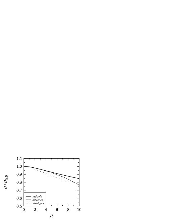
Figure 1: The pressure (scaled by the Stefan-Boltzmann pressure of an massless ideal gas) in our approach eq. (10) (full line) as a function of the coupling strength. The dotted line is the ideal massive gas contribution (first term in eq. (10)), while the dashed line depicts the result of the screened loop expansion [2].

References

-
[1]
P. Arnold, C. Zhai, Phys. Rev. D 50 (1994) 7603, D 51 (1995) 1906,
C. Zhai, B. Kastening, Phys. Rev. D 52 (1995) 7232,
E. Braaten, A. Nieto, Phys. Rev. D 53 (1996) 3421 - [2] F. Karsch, A. Patkos, P. Petreczky, Phys. Lett. B 401 (1997) 69
- [3] I.T. Drummond, R.R. Horgan, P.V. Landshoff, A. Rebhan, hep-ph/9708426
-
[4]
G. Boyd et al., Phys. Rev. Lett. 75 (1995) 419,
J. Engels et al., Phys. Lett. B 396 (1997) 210 - [5] A. Peshier, B. Kämpfer, O.P. Pavlenko, G. Soff, Phys. Rev. D 54 (1996) 2399
-
[6]
B. Kämpfer, O.P. Pavlenko, A. Peshier, M. Hentschel, G. Soff,
J. Phys. G 23 (1997) 2001,
P. Levai, U. Heinz, hep-ph/9710463 - [7] R.R. Parwani, H. Singh, Phys. Rev. D 51 (1995) 4518
- [8] T.D. Lee, C.N. Yang, Phys. Rev. 117 (1960) 22
- [9] J.M. Luttinger, J.C. Ward, Phys. Rev. 118 (1960) 1417
- [10] P. Fulde, H. Wagner, Phys. Rev. Lett. 27 (1971) 1280
- [11] R.E. Norton, J.M. Cornwall, Ann. Phys. 91 (1975) 106
- [12] A. Peshier, Ph.D. thesis, TU Dresden (1998), unpublished
- [13] F. Karsch, Nucl. Phys. B 9 [Proc. Suppl.] (1989) 357