FLAVOUR PHYSICS

Abstract

In these four lectures I review the theory and phenomenology of weak decays of quarks, and their rôle in the determination of the parameters of the Standard Model of particle physics, in testing subtle features of the theory and in searching for signatures of new physics. Attempts to understand $CP$-violation in current and future experiments is discussed.

1 Lecture 1: Introduction

Flavourdynamics, the study off the electroweak Lagrangian and its implications, is one of the central areas of research in particle physics. For example, in the United Kingdom the Mission Statement of the Particle Physics Community, as defined by our research council, is to obtain insights into the following three fundamental questions:

• the origin of mass,

• the 3 generations of elementary particles and their weak asymmetries,

• and

• the nature of dark matter.

The second of these topics is flavourdynamics, which is the subject of this lecture course. I will review the theoretical and experimental work being done in an attempt to determine the parameters of the Standard Model (SM) accurately, to test subtle properties of the SM and to define and search for signatures of New Physics. Although this primarily involves weak interactions, the major theoretical difficulty in interpreting experimental data on weak hadronic processes is controlling the non-perturbative strong interaction effects necessarily present in these decays. For this reason any review of flavour physics must contain a discussion also of these QCD effects, and much of the presentation below concerns this subject.

In the next few years much of the effort of the experimental community will be concerned with trying to gain an understanding of $CP$-violation. Indeed, one of the Sakharov conditions for generating a matter-antimatter asymmetry in the universe in the big-bang cosmology is the requirement for the existence of $CP$-violation. The existence of three generations of quarks and leptons, and hence of a complex phase in the mixing matrix, implies the presence of $CP$-violation at some level. Very little is known, however, about the value of this phase and hence of the magnitude of $CP$-violation induced by this mechanism, and also about other possible sources. It is hoped that the intensive studies, which are about to begin will significantly further our understanding and this will be one of the main topics of discussion towards the end of this lecture course.

The program for the four lectures is as follows:

1. The first lecture will be an introduction to weak decays in the Standard Model. Among the topics which will be covered will be charged and neutral currents, the Cabibbo-Kobayashi-Maskawa matrix and unitarity triangles, parity and charge conjugation symmetries, effective Hamiltonians and Operator Product Expansions and the Heavy Quark Effective Theory.

2. In the second lecture I will review the determination of the $V_{cb}$ and $V_{ub}$ matrix elements from semileptonic decays of $B$-mesons. Lattice computations, which provide the opportunity to evaluate non-perturbative strong interaction effects in weak decays in general, are introduced in this lecture.

3. The third lecture will contain a review of $K^{0}$-$\bar{K}^{0}$ and $B^{0}$-$\bar{B}^{0}$ mixing.

4. Finally, in the last lecture I review $CP$-violation in $B$-decays and the subject of inclusive $B$-decays.

The theoretical framework introduced in these lectures will be applied to several important physical processes. It will not be possible, however, to discuss the full range of interesting processes which are providing, or will provide, fundamental physical information. A much larger set of physical quantities is considered in detail in the beautiful review by Buras and Fleischer [1], to which I refer the student, and from which I will quote extensively. I also refer the reader to ref. [2] for a broad introduction to the Dynamics of the Standard Model and to references [3] and [4] for modern reviews of $B$-decays and $CP$-violation respectively. I will assume a familiarity with elementary Quantum Field Theory (as discussed for example by J. Petersen and V. Zakharov at this school [5]), but will try to avoid technical complexities, focussing instead on the underlying ideas.

1.1 The Interactions of Quarks and Gauge Bosons

Figure 1: The basic vertices representing the interactions of the quarks with the gauge bosons. The labels $i$ and $j$ represent the flavour quantum number ($i,j=u,d,c,s,t,b$).

The interactions between the quarks and gauge bosons in the Standard Model are illustrated in Fig. 1. In these lectures we will be particularly interested in the weak interactions. The vertex for the charged current interaction in which quark flavour $i$ changes to $j$ is depicted in Fig 1(a) and has the Feynman rule

$$i\frac{g_{2}}{2\sqrt{2}}V_{ij}\gamma_{\mu}(1-\gamma_{5})\ ,$$ (1)

where $g_{2}$ is the coupling constant of the $SU(2)_{L}$ gauge group and $V_{ij}$ is the $ij$ element of the Cabibbo-Kobayashi-Maskawa (CKM) matrix ($V_{ji}=V_{ij}^{*}$) [6]. Eq. (1) illustrates the $V{-}A$ (vector${-}$axial-vector) structure of the charged-current interactions.

At low energies, so that the momentum in the $W$-boson is much smaller than its mass $M_{W}$, the four-fermion interaction mediated by the $W$-boson can be approximated by the local Fermi $\beta$-decay interaction with coupling $G_{F}$, where

$$\frac{G_{F}}{\sqrt{2}}=\frac{g_{2}^{2}}{8M_{W}^{2}}\ ,$$ (2)

(see Fig. 2).

Figure 2: Approximation of the $W$-exchange interaction, by the four-fermion current-current vertex.

1.2 CKM - Matrix

The charged-current interactions are of the form

$$J_{\mu}^{CC}=(\bar{u},\bar{c},\bar{t})_{L}\gamma_{\mu}V_{\mathrm{CKM}}\left(\begin{array}[]{c}d\\ s\\ b\end{array}\right)_{\!\!\!L}\ ,$$ (3)

where (assuming the Standard Model with 3 generations) the CKM-matrix, $V_{\mathrm{CKM}}$ is a unitary 3$\times$ 3 one, relating the weak and mass eigenstates. The 1996 particle data book [7] gives the following values for the magnitudes of each of the elements:

$$\left(\begin{array}[]{ccc}0.9745-0.9757&0.219-0.224&0.002-0.05\\ 0.218-0.224&0.9736-0.9750&0.036-0.046\\ 0.004-0.014&0.034-0.046&0.9989-0.9993\end{array}\right)\ .$$ (4)

The subscript $L$ in eq. (3) represents left handed, ($\psi_{L}=\frac{1}{2}(1-\gamma^{5})\psi$).

If we have $2N_{g}$ quark flavours, ($N_{g}$ is the number of generations) then $V_{\mathrm{CKM}}$ is a $N_{g}\times N_{g}$ unitary matrix. It therefore has $N_{g}^{2}$ real parameters, however $(2N_{g}-1)$ of these can be absorbed into unphysical phases of the quark fields , leaving $(N_{g}-1)^{2}$ physical parameters to be determined.

In the two flavour case there is just one parameters, which is conventionally chosen to be the Cabibbo angle:

$$\left(\begin{array}[]{rr}\cos\theta_{c}&\ \sin\theta_{c}\\ -\sin\theta_{c}&\ \cos\theta_{c}\end{array}\right)$$ (5)

With three flavours there are 4 real parameters. Three of these can be interpreted as angles of rotation in three dimensions (e.g. the three Euler angles) and the fourth is a phase. The general parametrisation recommended by the Particle Data Group [7] is

$$\left(\begin{array}[]{ccc}c_{12}c_{13}&s_{12}c_{13}&s_{13}\exp(-i\delta_{13})\\ -s_{12}c_{23}-c_{12}s_{23}s_{13}\exp(i\delta_{13})&c_{12}c_{23}-s_{12}s_{23}s_{13}\exp(i\delta_{13})&s_{23}c_{13}\\ s_{12}s_{23}-c_{12}c_{23}s_{13}\exp(i\delta_{13})&-c_{12}s_{23}-s_{12}c_{23}s_{13}\exp(i\delta_{13})&c_{23}c_{13}\end{array}\right)$$ (6)

where $c_{ij}$ and $s_{ij}$ represent the cosines and sines respectively of the three angles $\theta_{ij}$, $ij=12,\,13\,23$. $\delta_{13}$ is the phase parameter.

The parametrisation in eq. (6) is general, but awkward to use. For most practical purposes it is sufficient to exploit the empirical fact that the elements get smaller as one moves away from the diagonal of the matrix (see eq. (4) ), and to use a simpler, but approximate parametrisation. It has become conventional to use the Wolfenstein parametrisation [8]:

$$V_{\mathrm{CKM}}=\left(\begin{array}[]{ccc}1-\frac{\lambda^{2}}{2}&\lambda&A\lambda^{3}(\rho-i\eta)\\ -\lambda&1-\frac{\lambda^{2}}{2}\rule{0.0pt}{14.0pt}&A\lambda^{2}\\ A\lambda^{3}(1-\rho-i\eta)&-A\lambda^{2}\rule{0.0pt}{14.0pt}&1\end{array}\right)\ .$$ (7)

$\lambda$ is approximately the Cabibbo angle, and the terms which are neglected in the Wolfenstein parametrisation are of $O(\lambda^{4})$. Much of the current effort of the particle physics community is devoted to determining the four parameters $\lambda,A,\rho$ and $\eta$, with ever increasing precision, and this will continue for some time to come. For this reason I will spend a significant fraction of these lectures on the theoretical issues related to the determination of these parameters.

From the unitarity of the CKM-matrix we have a set of relations between the entries. A particularly useful one is:

$$V_{ud}V_{ub}^{*}+V_{cd}V_{cb}^{*}+V_{td}V_{tb}^{*}=0\ .$$ (8)

In terms of the Wolfenstein parameters, the components on the left-hand side of eq. (8) are given by:

$$V_{ud}V_{ub}^{*} = A\lambda^{3}[\bar{\rho}+i\bar{\eta}]+O(\lambda^{7})$$

$$V_{cd}V_{cb}^{*} = -A\lambda^{3}+O(\lambda^{7})$$ (9)

$$V_{td}V_{tb}^{*} = A\lambda^{3}[1-(\bar{\rho}+i\bar{\eta})]+O(\lambda^{7})\ ,$$

where $\bar{\rho}=\rho(1-\lambda^{2}/2)$ and $\bar{\eta}=\eta(1-\lambda^{2}/2)$. The unitarity relation in eq. (8) can be represented schematically by the famous “unitarity triangle” of Fig. 3 (obtained after scaling out a factor of $A\lambda^{3}$).

Figure 3: Unitarity Triangle corresponding to the relation in eq. (8).

The notation in Fig. 3 is standard, and in the following lectures I will describe current and future attempts to determine the position of the vertex $A$, and hence the values of the angles $\alpha,\beta$ and $\gamma$. By using many different processes to overdetermine the position of $A$, one will be able to test the consistency of the SM, and check for evidence of physics beyond this model.

1.2.1 The Cabibbo Sector

Although much of the remainder of these lectures will be devoted to the determination of the entries in the CKM-matrix, since the Cabibbo sector is the best determined, I will not consider it beyond this subsection. I briefly review the status of the four entries in the $2\times 2$ top-left submatrix of $V_{\mathrm{CKM}}$ [7].

Figure 4: Subprocesses from which the $V_{ud}$, $V_{us}$, $V_{cd}$, and $V_{cs}$ elements of the CKM-Matrix are determined (see text).

• $\mathbf{V_{ud}}$:

  $$|V_{ud}|=0.9736\pm 0.0010\ .$$ (10)

  This is the best determined of the elements and is obtained by studying superallowed $\beta$-decays in nuclei (see fig. 4(a)). Since the publication of the 1996 particle data book, a result with a smaller error has been presented, $|V_{ud}|=0.9740\pm 0.0005$ [9].

• $\mathbf{V_{us}}$:

  $$|V_{us}|=\lambda=0.2205\pm 0.0018\ .$$ (11)

  This matrix element is obtained from semileptonic decays of $K$-mesons ($K^{+}\to\pi^{0}e^{+}\nu_{e}$, $K^{0}_{L}\to\pi^{-}e^{+}\nu_{e}$, see fig. 4(b) ) or of hyperons. In the $K$-meson decays, parity symmetry implies that only the vector component of the $V{-}A$ current contributes to the decays. Since the momentum transfer to the $\pi$-meson is small, and the vector current for degenerate quarks is conserved, the uncertainties due to strong interaction effects are small and can be estimated using chiral perturbation theory.

• $\mathbf{V_{cd}}$:

  $$|V_{cd}|=0.224\pm 0.016\ .$$ (12)

  The $V_{cd}$ element is obtained from charm production in deep inelastic neutrino (or antineutrino) nucleon scattering, see fig. 4(c).

• $\mathbf{V_{cs}}$:

  $$|V_{cs}|=1.01\pm 0.18\ .$$ (13)

  This matrix element can be determined from semileptonic decays of charmed mesons (see fig. 4(d)). In this case the large difference in the masses of the quarks make it difficult to estimate the strong interaction effects accurately (see sec. 2.1), and this is the reason for the relatively large error.

The errors in eqs. (10)-(13) are those in the measurements of these matrix elements themselves. Comparing these uncertainties with those in eq. (4), where the constraints of unitarity have been imposed (assuming just three generations), we see how much these constraints reduce the errors.

1.3 Flavour Changing Neutral Currents

In the Standard Model, unitarity implies that there are no Flavour Changing Neutral Current (FCNC) reactions at tree level, i.e. that there are no vertices of the type:

Quantum loops can, however, generate FCNC reactions, through box diagrams (see fig. 5) or penguin diagrams (see fig. 6), and we will discuss some of the physical processes induced by these loop-effects in the following lectures.

Figure 5: Box diagrams which contribute to the process of $B^{0}$-$\bar{B}^{0}$ mixing.

Figure 6: Examples of penguin diagrams which contribute to the FCNC process $d\to s$. Diagrams (a) and (b) are electroweak penguins graphs, whereas diagram (c) is a gluonic penguin graph.

As a consequence of the “GIM”-mechanism [10] all the FCNC vertices vanish in the limit of degenerate quark masses. This is a consequence of the unitarity of the CKM-matrix. For example, consider the vertex in the diagram of fig. 6(a), in the hypothetical situation in which there is a “horizontal” symmetry such that $m_{u}=m_{c}=m_{t}$. In this case the contribution from each of the positively charged quarks in the loop is simply proportional to the corresponding CKM-matrix elements, so that the total contribution is

$$V_{ud}V_{us}^{*}+V_{cd}V_{cs}^{*}+V_{td}V_{ts}^{*}$$ (14)

which vanishes by unitarity of the CKM-matrix. A similar argument holds for all the FCNC vertices.

Of course, in reality the masses of the quarks are not equal and the FCNC vertices are not zero. Depending on the process being studied, however, the GIM-mechanism may lead to a suppression of the amplitude.

1.4 $P$, $C$ and $CP$ Symmetries

Symmetries play a fundamental rôle in physics in general and in particle physics in particular. In this subsection I briefly introduce the violation of $CP$-symmetry, which will be a focus of many of the studies at $B$-physics facilities in the next few years.

Parity:

The parity transformation reverses the sign of spatial coordinates, $(\mathbf{x},t)\to(-\mathbf{x},t)$. The vector and axial-vector fields transform as:

$$V_{\mu}(\mathbf{x},t)\to V^{\mu}(-\mathbf{x},t)\ \ \textrm{and}\ \ \ A_{\mu}(\mathbf{x},t)\to-A^{\mu}(-\mathbf{x},t)\ ,$$ (15)

and the vector and axial-vector currents transform similarly. Left-handed components of fermions $(\frac{1}{2}(1-\gamma^{5})\psi)$ transform into right-handed ones $(\frac{1}{2}(1+\gamma^{5})\psi)$, and vice-versa. Since weak interactions only involve the left-handed components, parity is not a good symmetry of the weak force, in distinction to the strong and electromagnetic forces (QCD and QED are invariant under parity transformations).

Charge Conjugation:

For free fields ($\phi(x)$ say) we can perform a fourier decomposition, with coefficients which contain annihilation and creation operators:

$$\phi(x)=\ \cdots\ a\ +\ \cdots\ b^{\dagger}\ ,$$ (16)

where $a$ and $b^{\dagger}$ represent the annihilation and creation operators for the particle and antiparticle. The charge conjugation transformation is the interchange of $a$ and $b$. In an interacting field theory this is not in general the same as interchanging physical particles and antiparticles for which we need the $CPT$ combined transformation ($T$ is time reversal transformation). Nevertheless $C$-tranformations are also interesting in field theories. Under $C$ the currents transform as follows:

$$\bar{\psi}_{1}\gamma_{\mu}\psi_{2}\to-\bar{\psi}_{2}\gamma_{\mu}\psi_{1}\ \ \ \textrm{and}\ \ \ \bar{\psi}_{1}\gamma_{\mu}\gamma_{5}\psi_{2}\to\bar{\psi}_{2}\gamma_{\mu}\gamma_{5}\psi_{1}\ ,$$ (17)

where $\psi_{i}$ represents a spinor field of type (flavour or lepton species) $i$.

$\mathbf{CP:}$

Under the combined $CP$-transformation, the currents transforms as:

$$\bar{\psi}_{1}\gamma_{\mu}\psi_{2}\to-\bar{\psi}_{2}\gamma^{\mu}\psi_{1}\ \ \ \textrm{and}\ \ \ \bar{\psi}_{1}\gamma_{\mu}\gamma_{5}\psi_{2}\to-\bar{\psi}_{2}\gamma^{\mu}\gamma_{5}\psi_{1}\ ,$$ (18)

where the fields on the left (right) hand side are evaluated at $(\mathbf{x},t)$ ( $(-\mathbf{x},t)$ ). Consider now a charged current interaction:

$$(W_{\mu}^{1}-iW^{2}_{\mu})\,\bar{U}^{i}\gamma^{\mu}(1-\gamma^{5})V_{ij}D^{j}+(W_{\mu}^{1}+iW^{2}_{\mu})\,\bar{D}^{j}\gamma^{\mu}(1-\gamma^{5})V_{ij}^{*}U^{i}\ ,$$ (19)

where $W$ represents the field of the $W$-boson and $U^{i}$ and $D^{j}$ are up and down type quarks of flavours $i$ and $j$ respectively. Under a $CP$ transformation, the interaction term in eq. (19) transforms to:

$$(W_{\mu}^{1}+iW^{2}_{\mu})\,\bar{D}^{j}\gamma^{\mu}(1-\gamma^{5})V_{ij}U^{i}+(W_{\mu}^{1}-iW^{2}_{\mu})\,\bar{U}^{i}\gamma^{\mu}(1-\gamma^{5})V_{ij}^{*}D^{j}\ ,$$ (20)

where the parity transformation on the coordinates is implied. Comparing eqs. (19) and (20), we see that $CP$-conservation requires the CKM-matrix $V_{ij}$ to be real (or more strictly that any phases must be absorbable into the definition of the quark fields). If the only source of $CP$-violation in nature is the phase in the CKM-matrix, then at least three generations of quarks are required (see subsec. 1.2). A central element of the research of the forthcoming generation of experiments in $B$-physics will be to determine whether the phase in the CKM-matrix is the only (or the main) source of $CP$-violation.

$CP$-violation appears to be small compared to the strength of the weak interaction, so that $CP$ is a fairly good symmetry. We recall that the presence of CP-violation is one of the Sakharov conditions for the creation of the baryon-antibaryon asymmetry of the universe.

1.5 Leptonic Decays of Mesons

As already mentioned, the main difficulty in making predictions for weak decays of hadrons is in controlling the non-perturbative strong-interaction effects. We will encounter this problem several times in subsequent lectures, but, as an introduction, I now discuss it briefly in a particularly simple situation, that of the leptonic decays of pseudoscalar mesons in general, and of the $B$-meson in particular.

Figure 7: Diagram representing the leptonic decay of the $B$-meson.

The leptonic decay of a pseudoscalar meson (e.g. the $B$-meson) is illustrated in the diagram of Fig. 7. All the QCD effects corresponding to the strong interactions between the quarks in Fig. 7 are contained in the matrix element of the $V{-}A$ hadronic current:

$$\langle 0|\,\bar{b}\gamma^{\mu}(1-\gamma^{5})u\,|B(p)\rangle\ .$$ (21)

Lorentz and parity symmetries imply that the matrix element of the vector component of the $V{-}A$ current vanishes ($\langle 0|\,\bar{b}\gamma^{\mu}u\,|B(p)\rangle=0$). This component is an axial-vector, and there is no axial-vector which can be constructed from the single vector we have at our disposal ($p$) and the invariant tensors ($g^{\mu,\nu}$ and $\varepsilon^{\mu\nu\rho\sigma}$). These symmetries also imply that the matrix element of the axial component of the $V{-}A$ current is a Lorentz-vector, and hence that it is proportional to $p^{\mu}$:

$$\langle 0|\,\bar{b}\gamma^{\mu}\gamma^{5}u\,|B(p)\rangle=if_{B}p^{\mu}\ .$$ (22)

The constant of proportionality, $f_{B}$, is called the decay constant of the $B$-meson. Thus all the QCD-effects for leptonic decays of $B$-mesons are contained in a single number, $f_{B}$. An identical discussion holds for other pseudoscalar mesons ($\pi,K,\cdots$). The normalisation used throughout these lectures, corresponds to $f_{\pi}\simeq 132$ MeV ($f_{B}$ is unknown at present). For leptonic decays of vector mesons, space-time symmetries also imply that the strong interaction effects are contained in a single decay constant. Thus, the rôle of quantitative non-perturbative methods, such as lattice QCD (discussed in sec. 2.3 below) or QCD sum-rules, is to provide the framework for the evaluation of matrix elements such as that in eq. (21).

1.6 Operator Product Expansions and Effective Hamiltonians

Even though this is a course in flavour physics, we cannot avoid the fact that the quarks are interacting strongly and hence that QCD effects must be considered. Indeed, as already mentioned above, our rather primitive control of non-perturbative QCD is the principal source of uncertainty in interpeting experimental data of weak decays and in determining the fundamental parameters of the Standard Model.

In Paolo Nason’s lecture course [11], we have seen how the property of asymptotic freedom, which states that the interactions of quarks and gluons become weaker at short distances, enables us to use perturbation theory to make predictions for a wide variety of short-distance (or light-cone) dominated processes. For separations $|x|\ll\Lambda_{QCD}^{-1}$ ( $|x|<0.1$ fm say) or corresponding momenta $|p|\gg\Lambda_{QCD}$ ( $|p|>2$ GeV say), we can use perturbation theory. The natural scale of strong interaction physics is of $O(1~{}\textrm{fm})$, however, and so in general, and for most of the processes discussed in this course, non-perturbative techniques must be used.

Figure 8: Diagrams contributing to hadronic decays of $K$-mesons

As an example, consider a decay of a $K$-meson into two pions, for which a tree-level diagram of the quark subprocess is depicted in Fig. 8(a). The amplitude is proportional to

$$\frac{G_{F}}{\sqrt{2}}\,V_{ud}^{*}V_{us}\,\langle\pi\pi|(\bar{d}\gamma^{\mu}(1-\gamma^{5})u)\,(\bar{u}\gamma_{\mu}(1-\gamma^{5})s)|K\rangle\ ,$$ (23)

i.e. it is proportional to the matrix element of the operator

$$O_{1}=(\bar{d}\gamma^{\mu}(1-\gamma^{5})u)\,(\bar{u}\gamma_{\mu}(1-\gamma^{5})s)$$ (24)

between $|K\rangle$ and $|\pi\pi\rangle$ states. A one-loop (i.e. one-gluon exchange) correction to this diagram is shown in Fig. 8(b). This clearly generates a second operator, $(\bar{d}T^{a}\gamma^{\mu}(1-\gamma^{5})u)\,(\bar{u}T^{a}\gamma_{\mu}(1-\gamma^{5})s)$ , which, using Fierz identities can be written as a linear combination of $O_{1}$ and $O_{2}$ where

$$O_{2}=(\bar{d}\gamma^{\mu}(1-\gamma^{5})s)\,(\bar{u}\gamma_{\mu}(1-\gamma^{5})u)\,.$$ (25)

This discuusion can be generalized to higher orders, as I now explain.

Using the operator product expansion (OPE) one writes the amplitude for a weak decay process from an initial state $\mathcal{I}$ to a final state $\mathcal{F}$ in the form:

$$T_{\mathcal{F}I}=\frac{G_{F}}{\sqrt{2}}\,V_{CKM}\,\sum_{i}C_{i}(\mu)\langle\mathcal{F}|\,O_{i}(\mu)\,|\mathcal{I}\rangle\ .$$ (26)

$\mu$ is the renormalization scale at which the composite operators $O_{i}$ are defined and $V_{CKM}$ is the appropriate product of CKM-matrix elements. The expansion (26) is very convenient. The non-perturbative QCD effects are contained in the matrix elements of the operators $O_{i}$, which are independent of the large momentum scale, in this case of $M_{W}$. The Wilson coefficient functions $C_{i}(\mu)$ are independent of the states $\mathcal{I}$ and $\mathcal{F}$ and can be calculated in perturbation theory. Since physical amplitudes manifestly do not depend on $\mu$, the $\mu$-dependence in the operators $O_{i}(\mu)$ is cancelled by that in the coefficient functions $C_{i}(\mu)$. The effective Hamiltonian for weak decays can then be written in the form:

$$\mathcal{H}_{\mathrm{eff}}\equiv\frac{G_{F}}{\sqrt{2}}\,V_{CKM}\,\sum_{i}C_{i}(\mu)\,O_{i}(\mu)\ .$$ (27)

In order to gain a little further intuition into the origin of eq.(26) consider the one-loop graph of Fig. 8(b). Dimensional counting at large loop momenta $k$ readily shows that the graph is ultra-violet convergent (in the Feynman gauge, say):

$$\int_{k\mathrm{\ large}}\frac{1}{k}\ \frac{1}{k}\ \frac{1}{k^{2}}\ \frac{1}{k^{2}-M_{W}^{2}}\ d^{4}k\ ,$$ (28)

where the first two factors in the integrand ($1/k$) correspond to the two quark propagators, the third ($1/k^{2}$) to the gluon propagator and the final factor to the propagator of the $W$-boson. It can be deduced from eq.(28) that the contribution from this graph contains a term proportional to $\log(M_{W}^{2}/p^{2})$, where p is some low-momentum (infra-red) scale.

Figure 9: One-loop correction to the Green function of the operator $O_{1}$.

Consider now the one-loop graph of Fig. 9, depicting a correction to a matrix element of the operator $O_{1}$ defined in eq. (24). Now the $W$-propagator is absent, and the power counting in the large momentum region gives:

$$\int_{k\mathrm{\ large}}\frac{1}{k}\ \frac{1}{k}\ \frac{1}{k^{2}}\ d^{4}k\ ,$$ (29)

i.e. a logarithmically divergent contribution. After renormalization at a scale $\mu$ there will be a contribution to this graph proportional to $\log(\mu^{2}/p^{2})$. In the low momentum (non-perturbative) region (i.e. for $|k_{\mu}|\ll M_{W}$) the contributions from the graphs in Figs. 8(b) and 9 are the same. Thus we can split the factor of $\log(M_{W}^{2}/p^{2})$ from the graph of Fig. 8(b) into two parts; the first, $\log(\mu^{2}/p^{2})$ is contained in the matrix element of $O_{1}$, and the second, $\log(M_{W}^{2}/\mu^{2})$, into the coeficient function $C_{1}$. Since the infra-red behaviour of the graphs in Figs. 8(b) and 9 are the same, the coefficient functions are independent of the treatment of the low-momentum region. Moreover, in order to calculate the coefficient functions, we can choose any convenient external states, and in practice one chooses quark or gluon states. We refer to the evaluation of the coefficient functions as the process of matching.

In $K$-decays it is natural, although not necessary, to choose $\mu$ to be as small as one can without invalidating perturbation theory. In this way one might hope to avoid large logarithms ($\log(\mu^{2}/p^{2}$) ) which would spoil any insights we might have about the operator matrix elements from non-relativistic quark models or other approaches. Of course this implies the presence of large logarithms of the type $\alpha_{s}^{n}\log^{n}(M_{W}^{2}/\mu^{2})$ in the coefficient functions, but these can be summed using the renormalization group, leading to factors of the type:

$$\left[\frac{\alpha_{s}(M_{W})}{\alpha_{s}(\mu)}\right]^{\gamma_{0}/2\beta_{0}}\ ,$$ (30)

where $\gamma_{0}$ is the one-loop contribution to the anomalous dimension of the operator (proportional to the coefficient of $\log(\mu^{2}/p^{2})$ in the evaluation of the graph of fig. 8(b) ) and $\beta_{0}$ is the first term in the $\beta$-function, ($\beta\equiv\partial g/\,\partial\ln(\mu)\,=\,-\beta_{0}\,g^{3}/16\pi^{2}$) . Eq. (30) represents the sum of the leading logarithms, i.e. the sum of the terms $\alpha_{s}^{n}\log^{n}(M_{W}^{2}/\mu^{2})$. For almost all the important processes, the first (or even higher) corrections have also been evaluated.

We end this subsection by making some further points about the use of the OPE in weak decays and other hard processes:

• We shall see below that for some important physical quantities (e.g. $\epsilon^{\prime}/\epsilon$), there may be as many as ten operators, whose matrix elements have to be estimated.

• One may try to evaluate the matrix elements using some non-perturbative computational technique, such as lattice simulations or QCD sum-rules (see below), or to determine them from experimental data. In the latter case, if there are more measurements possible than unknown parameters (i.e. matrix elements), then one is able to make predictions.

• In weak decays the large scale, $M_{W}$, is of course fixed. For other processes, most notably for deep-inelastic lepton-hadron scattering, the OPE is useful in computing the behaviour of the amplitudes with the large scale (e.g. with the momentum transfer).

1.7 The Heavy Quark Effective Theory - HQET

Most of the important physical properties of the hydrogen atom are independent of the mass of the nucleus. Analogous features hold in the physics of heavy hadrons, where by heavy I mean that $m_{Q}\gg\Lambda_{QCD}$ and $m_{Q}$ is the mass of the heavy quark. During the last few years the construction and use of the Heavy Quark Effective Theory (HQET), has proved invaluable in the study of heavy quark physics. In this subsection I briefly introduce the main features of the HQET, which will be used in the following lectures.

Consider the propagator of a (free) heavy quark:

If the momentum of the quark $p$ is not far from its mass shell,

$$p_{\mu}=m_{Q}v_{\mu}+k_{\mu}\ ,$$ (31)

where $|k_{\mu}|\ll m_{Q}$ and $v_{\mu}$ is the (relativistic) four velocity of the hadron containing the heavy quark ($v^{2}=1$), then

$(1+\not{v})/2$ is a projection operator, projecting out the large components of the spinors. This propagator can be obtained from the gauge-invariant action

$$\mathcal{L}_{HQET}=\bar{h}(iv\cdot D)\frac{1+\not{v}}{2}h\ ,$$ (32)

where $h$ is the spinor field of the heavy quark . $\mathcal{L}_{HQET}$ is independent of $m_{Q}$, which implies the existence of symmetries relating physical quantities corresponding to different heavy quarks (in practice the $b$ and $c$ quarks). The light degrees of freedom are also not sensitive to the spin of the heavy quark, which leads to a spin-symmetry relating physical properties of heavy hadrons of different spins. Consider, for example, the correlation function:

$$\int d^{3}x\,\langle 0|J_{H}(x)\,J_{H}^{\dagger}(0)\,|0\rangle\ ,$$ (33)

where $J_{H}^{\dagger}$ ($J_{H}$) is an interpolating operator which can create a heavy hadron $H$, which we take to be a pseudoscalar or vector meson. The hadron is produced at rest, with four velocity $v=(\mathbf{0},1)$. We can use the interpolating operator $J_{H}=\bar{h}\gamma^{5}q$ for the pseudoscalar meson and $J_{H}=\bar{h}\gamma^{i}q$ ($i=1,2,3$) for the vector meson. This means that the correlation function will be identical in the two cases except for the factor

$$\gamma^{5}\frac{1+\gamma^{0}}{2}\gamma^{5}=\frac{1-\gamma^{0}}{2}$$ (34)

when $H$ is a pseudoscalar meson, and

$$\gamma^{i}\frac{1+\gamma^{0}}{2}\gamma^{i}=-3\,\frac{1-\gamma^{0}}{2}$$ (35)

when it is a vector meson. Since the correlation functions behave with time as $\exp(-iM_{H}t)$ , this implies that the pseudoscalar and vector mesons are degenerate, up to relative corrections of $O(\Lambda_{QCD}^{2}/m_{Q})$:

$$M_{P}=M_{V}+O(\Lambda_{QCD}^{2}/m_{Q})\ ,$$ (36)

where $M_{P}$ and $M_{V}$ are the masses of the pseudoscalar and vector mesons respectively, or equivalently

$$M_{V}^{2}-M_{P}^{2}=\textrm{constant}\ .$$ (37)

This relation is reasonably well satisfied experimentally:

$$M_{B^{*}}^{2}-M_{B}^{2}=0.485\,\textrm{GeV}^{2}\ \ \ \textrm{and}\ \ \ M_{D^{*}}^{2}-M_{D}^{2}=0.546\,\textrm{GeV}^{2}\ ,$$ (38)

which is encouraging. However, I also mention in passing that the light mesons, to which the HQET certainly does not apply, also satisfy these relations numerically:

$$M_{K^{*}}^{2}-M_{K}^{2}=0.552\,\textrm{GeV}^{2}\ \ \ \textrm{and}\ \ \ M_{\rho}^{2}-M_{\pi}^{2}=0.571\,\textrm{GeV}^{2}\ .$$ (39)

The usefulness of the HQET does not lie in the fact that the residual momenta $k$ are always much smaller than $\Lambda_{QCD}$; indeed this is not true, in QCD one does have hard gluons with arbitrarily large momenta. However the effects of hard gluons can be evaluated in perturbation theory. The non-perturbative strong interaction effects are the same in QCD and in the HQET (up to corrections of $O(\Lambda_{QCD}/m_{Q})$, which for the moment we neglect), and so the HQET relations, such as that between the decay constants of pseudoscalar and vector mesons, which can be deduced from the above proportionality of correlation functions, are violated only by perturbatively calculable corrections.

The principal application of the HQET is in $b$-physics, and to a lesser extent to charm physics. In both cases the corrections of $O(\Lambda_{QCD}/m_{Q})$ are significant, and hence one would like to compute these corrections. In practice, this gets progressively more difficult, and it is a much debated point as to whether even the first corrections (i.e. those of $O(\Lambda_{QCD}/m_{Q})$ relative to the leading terms) have been reliably calculated for any interesting quantity.

2 Lecture 2: $V_{cb}$ and $V_{ub}$

In this lecture I will discuss exclusive semileptonic decays of $B$-mesons, in which the $b$-quark decays into a $c$- or $u$-quark, and from which one can determine the $V_{cb}$ and $V_{ub}$ elements of the CKM-matrix. The decays are represented in Fig. 10. It is convenient to use space-time symmetries to express the matrix elements in terms of invariant form factors (using the helicity basis for these as defined below). When the final state is a pseudoscalar meson $P$, parity implies that only the vector component of the $V{-}A$ weak current contributes to the decay, and there are two independent form factors, $f^{+}$ and $f^{0}$, defined by

$$\langle P(k)|V^{\mu}|B(p)\rangle=f^{+}(q^{2})\left[(p+k)^{\mu}-\frac{m_{B}^{2}-m_{P}^{2}}{q^{2}}\,q^{\mu}\right]+f^{0}(q^{2})\,\frac{m_{B}^{2}-m_{P}^{2}}{q^{2}}\,q^{\mu}\ ,$$ (40)

where $q$ is the momentum transfer, $q=p{-}k$. When the final-state hadron is a vector meson $V$, there are four independent form factors, $V$, $A_{1}$, $A_{2}$ and $A$:

$$\langle V(k,\varepsilon)|V^{\mu}|B(p)\rangle = \frac{2V(q^{2})}{m_{B}+m_{V}}\epsilon^{\mu\gamma\delta\beta}\varepsilon^{*}_{\beta}p_{\gamma}k_{\delta}$$ (41)

$$\langle V(k,\varepsilon)|A^{\mu}|B(p)\rangle = i(m_{B}{+}m_{V})A_{1}(q^{2})\varepsilon^{*\,\mu}-i\frac{A_{2}(q^{2})}{m_{B}{+}m_{V}}\varepsilon^{*}\!\mathord{\cdot}p\,(p{+}k)^{\mu}$$ (42)

$$\mbox{}+i\frac{A(q^{2})}{q^{2}}2m_{V}\varepsilon^{*}\!\mathord{\cdot}p\,q^{\mu}\ ,$$

where $\varepsilon$ is the polarization vector of the final-state meson, and $q=p{-}k$. Below we shall also discuss the form factor $A_{0}$, which is given in terms of those defined above by $A_{0}=A+A_{3}$, with

$$A_{3}=\frac{m_{B}+m_{V}}{2m_{V}}A_{1}-\frac{m_{B}-m_{V}}{2m_{V}}A_{2}\ .$$ (43)

Figure 10: Diagram representing the semileptonic decay of the $B$-meson. $\bar{q}$ represents the light valence antiquark, and the black circle represents the insertion of the $V$–$A$ current with the appropriate flavour quantum numbers.

2.1 Semileptonic $B\to D$ and $B\to D^{*}$ Decays

Semileptonic $B\to D^{*}$ and, more recently, $B\to D$ decays are used to determine the $V_{cb}$ element of the CKM matrix. Heavy quark symmetry is rather powerful in controlling the theoretical description of these heavy-to-heavy quark transitions (see e.g. the review article by Neubert for details and references [12]).

In the heavy quark limit, all six form factors in eqs. (40) - (42) are related and there is just one universal form factor $\xi(\omega)$, known as the Isgur–Wise (IW) function, which contains all the non-perturbative QCD effects. Specifically:

$$f^{+}(q^{2})=V(q^{2})=A_{0}(q^{2})=A_{2}(q^{2})=\left[1-\frac{q^{2}}{(m_{B}+m_{D})^{2}}\right]^{-1}A_{1}(q^{2})=\frac{m_{B}+m_{D}}{2\sqrt{m_{B}m_{D}}}\,\xi(\omega)\ ,$$ (44)

where $\omega=v_{B}\mathord{\cdot}v_{D}$ is the velocity transfer variable ($v_{B,D}$ are the four velocities of the corresponding mesons). Here the label $D$ represents the $D$- or $D^{*}$-meson as appropriate (pseudoscalar and vector mesons are degenerate in this leading approximation). Vector current conservation implies that the IW-function is normalized at zero recoil, i.e. that $\xi(1)=1$. This property is particularly important in the extraction of $V_{cb}$.

To get some insights into the origin of the heavy quark relations above, let us consider $B\to D$ decays. We can rewrite eq. (40) in terms of the form factors $f^{+}$ and $f^{-}$ (instead of using the helicity basis as in eq. (40) ):

$$\langle D(p^{\prime})|\bar{c}\gamma^{\mu}b|B(p)\rangle=f^{+}(q^{2})(p+p^{\prime})^{\mu}-f^{-}(q^{2})(p-p^{\prime})^{\mu}\ ,$$ (45)

where $q=p-p^{\prime}$. Defining the four-velocities $v$ and $v^{\prime}$ by $p=m_{B}\,v$ and $p^{\prime}=m_{D}\,v^{\prime}$, eq. (45) can be rewritten as:

$$\langle D(v^{\prime})|\,\bar{c}\gamma^{\mu}b\,|B(v)\rangle = \frac{1}{2}\left[(m_{B}+m_{D})f^{+}(q^{2})-(m_{B}-m_{D})f^{-}(q^{2})\right](v+v^{\prime})^{\mu}$$ (46)

$$\hskip 36.135pt+\frac{1}{2}\left[(m_{B}-m_{D})f^{+}(q^{2})-(m_{B}+m_{D})f^{-}(q^{2})\right](v-v^{\prime})^{\mu}\ .$$

Now in the HQET:

$$\sqrt{m_{B}m_{D}}\,\langle P(v^{\prime})|\,\bar{h}_{v^{\prime}}\gamma^{\mu}h_{v}\,|P(v)\rangle=\sqrt{m_{B}m_{D}}\,\xi(\omega)\,(v+v^{\prime})^{\mu}\ ,$$ (47)

where $\omega=v\mathord{\cdot}v^{\prime}$, and the projection operators (e.g. $(1+\not\!\!\!v)/2$) have been absorbed into the heavy quark fields. $P$ represents a heavy pseudoscalar meson, and the factors $\sqrt{m_{B}m_{D}}$ are chosen in order to introduce a mass-independent normalization of states (so that the matrix elements are independent of any masses). There is no term proportional to $(v-v^{\prime})^{\mu}$ on the right hand side of eq. (47), since $\bar{h}_{v^{\prime}}(\not\!v-\not\!v^{\prime})h_{v}=0$, and so we obtain the relations:

$$f^{-}=\frac{m_{B}-m_{D}}{m_{B}+m_{D}}f^{+}\ \ \ \textrm{and}\ \ \ f^{\pm}=\frac{m_{B}\pm m_{D}}{2\sqrt{m_{B}m_{D}}}\,\xi(\omega)\ .$$ (48)

To understand the normalization condition $\xi(1)=1$, consider the forward matrix element:

$$\langle B(p)|\,\bar{b}\gamma^{\mu}b\,|B(p)\rangle=2p^{\mu}f^{+}(0)=2p^{\mu}\ ,$$ (49)

where the last relation follows from the conservation of the current $\bar{b}\gamma^{\mu}b$ which implies that $f^{+}(0)=1$. In the HQET this matrix element is equal to $m_{B}\,2v^{\mu}\,\xi(1)$, and so $\xi(1)=1$. The spin symmetry relates the form-factors of $B\to D^{*}$ decays to $\xi(\omega)$.

The relations in eq. (44) are valid up to perturbative and power corrections. The precision with which $V_{cb}$ can be extracted is limited by the theoretical uncertainties in the evaluation of these corrections. Nevertheless we are in the fortunate situation that it is uncertainties in corrections (which are therefore small) which control the precision.

Allowing for these corrections to the results in the heavy quark limit, one writes the decay distribution for $B\to D^{*}$ decays as:

$$\frac{d\Gamma}{d\omega}=\frac{G_{F}^{2}}{48\pi^{3}}(m_{B}{-}m_{D^{*}})^{2}m_{D^{*}}^{3}\sqrt{\omega^{2}{-}1}\,(\omega{+}1)^{2}\left[1+\frac{4\omega}{\omega{+}1}\frac{m_{B}^{2}-2\omega m_{B}m_{D^{*}}+m_{D^{*}}^{2}}{(m_{B}-m_{D^{*}})^{2}}\right]|V_{cb}|^{2}\,{\cal F}^{2}(\omega)\ ,$$ (50)

where ${\cal F}(\omega)$ is the IW-function combined with perturbative and power corrections. It is convenient theoretically to consider this distribution near $\omega=1$, in order to exploit the normalization condition $\xi(1)=1$. In this case there are no $O(1/m_{Q})$ corrections (where $Q=b$ or $c$) by virtue of Luke’s theorem [13], so that the expansion of $\mathcal{F}(1)$ begins like:

$${\cal F}(1)=\eta_{A}\left(1+0\,\frac{\Lambda_{QCD}}{m_{Q}}+c_{2}\frac{\Lambda^{2}_{QCD}}{m_{Q}^{2}}+\cdots\right)\,,$$ (51)

where $\eta_{A}$ represents the perturbative corrections. The one-loop contribution to $\eta_{A}$ has been known for some time now, whereas the two-loop contribution was evaluated last year, with the result [14]:

$$\eta_{A}=0.960\pm 0.007\ ,$$ (52)

where I have taken the value of the two loop contribution as an estimate of the error.

The power corrections are much more difficult to estimate reliably. Neubert has recently combined the results of refs. [15, 16, 17] to estimate that the $O(1/m_{Q}^{2})$ terms in the parentheses in eq. (51) are about $-0.055\pm 0.025$ and that ${\cal F}(1)=0.91(3)\,$. Bigi, Shifman and Uraltsev [18], consider the uncertainties to be bigger and obtain $0.91(6)$. Combining the latter, more cautious, theoretical value of ${\cal F}(1)$, with the experimental result [19] ${\cal F}(1)|V_{cb}|=(34.3\pm 1.6)10^{-3}$, readily gives $|V_{cb}|=(37.7\pm 1.8_{exp}\pm 2.5_{th})10^{-3}$.

Here I am only discussing exclusive decays. Buras and Fleischer, perform an analysis of both exclusive and inclusive semileptonic decays and quote $V_{cb}=(40\pm 3)\,10^{-3}$ as their best value [1].

$|V_{cb}|$ gives the scale of the unitarity triangle:

$$\lambda\,|V_{cb}|=\lambda^{3}A\ .$$ (53)

2.2 Semileptonic $B\to\pi$ and $B\to\rho$ Decays

In this subsection we consider the heavy-to-light semileptonic decays $B\to\rho$ and $B\to\pi$ which are now being used experimentally to determine the $V_{ub}$ matrix element [20, 21]. Heavy quark symmetry is less predictive for heavy-to-light decays than for heavy-to-heavy ones. In particular, there is no normalization condition at zero recoil corresponding to the condition $\xi(1)=1$, which is so useful in the extraction of $V_{cb}$ (see subsection 2.1). The lack of such a condition puts a premium on the results from nonperturbative calculational techniques, such as lattice QCD or light-cone sum rules. Heavy quark symmetry does, however, give useful scaling laws for the behaviour of the form factors with the mass of the heavy quark ($m_{Q}$) at fixed $\omega$:

$$f^{+},A_{0},A_{2},V\sim\sqrt{m_{Q}}\ ;\ A_{1},f^{0}\sim\frac{1}{\sqrt{m_{Q}}}\ ;\ A_{3}\sim m_{Q}^{\frac{3}{2}}\ .$$ (54)

These scaling relations are particularly useful in lattice simulations, where the masses of the quarks are varied. Moreover, the heavy quark spin symmetry relates the $B\to V$ matrix elements [22, 23] (where $V$ is a light vector particle) of the weak current and magnetic moment operators, thereby relating the amplitudes for the two physical processes $\bar{B}^{0}\to\rho^{+}l^{-}\bar{\nu}_{l}$ and $\bar{B}\to K^{*}\gamma$, up to $SU(3)$ flavour symmetry breaking effects. These relations also provide important checks on theoretical, and in particular on lattice, calculations.

Recent compilations of results for $|V_{ub}/V_{cb}|$, include 0.06-0.11 obtained from exclusive decays only (or $0.08\pm 0.01_{\mbox{exp}}\pm 0.02_{\mbox{th}}$ from inclusive decays) [12, 24] and $0.08\pm 0.02$ from both inclusive and exclusive decays [1]. In terms of the parameters of the unitarity triangle (see fig. 3):

$$CA=\frac{|V_{ud}V_{ub}^{*}|}{|V_{cd}V_{cb}^{*}|}=\sqrt{\bar{\rho}^{2}+\bar{\eta}^{2}}=(1-\frac{\lambda^{2}}{2})\frac{1}{\lambda}\frac{|V_{ub}|}{|V_{cb}|}\simeq 4.44\,\frac{|V_{ub}|}{|V_{cb}|}\ .$$ (55)

Thus a measurement of $|V_{ub}/V_{cb}|$ implies that the locus of possible positions of the vertex $A$ is a circle centred on $C$ (see fig. 11). In practice, of course, because of the theoretical and experimental uncertainties, the circle is replaced by a band.

Figure 11: A precise determination of $|V_{ub}/V_{cb}|$ would fix the vertex $A$ to lie on a given circle centered on $C$ (schematically represented by the solid line).

2.3 Lattice QCD

We have seen that the main difficulty in making predictions for weak hadronic decays is our inability to control the long-distance strong interaction effects present in these decays. The principal technique for the evaluation of these non-perturbative effects is lattice QCD, and I now digress from the main theme of this course to outline briefly the principles underlying lattice calculations of non-perturbative QCD effects in weak decays and to discuss the main sources of uncertainty present in these computations.

In subsection 1.6 we have seen that, by using the Operator Product Expansion, it is generally possible to separate the short- and long-distance contributions to weak decay amplitudes into Wilson coefficient functions and operator matrix elements respectively. Thus, in order to evaluate the non-perturbative QCD effects, it is necessary to compute the matrix elements of local composite operators. This is achieved in lattice simulations, by the direct computation of correlation functions of multi-local operators composed of quark and gluon fields (in Euclidean space):

$$\langle 0|\,O(x_{1},x_{2},\ldots,x_{n})|0\rangle=\,\frac{1}{Z}\int[DA_{\mu}][D\psi][D\bar{\psi}]\,e^{-S}\,O(x_{1},x_{2},\ldots,x_{n})\ ,$$ (56)

where $Z$ is the partition function

$$Z=\int[DA_{\mu}][D\psi][D\bar{\psi}]\,e^{-S}\ ,$$ (57)

$S$ is the action and the integrals are over quark and gluon fields at each space-time point. In eq. (56) $O(x_{1},x_{2},\ldots,x_{n})$ is a multi-local operator; the choice of $O$ governs the physics which can be studied.

We now consider the two most frequently encountered cases, for which $n{=}2$ or $3$. As a first example, let $O(x_{1},x_{2})$ be the bilocal operator

$$O_{2}(x_{1},x_{2})=T\{J_{H}(x_{1})J^{\dagger}_{H}(x_{2})\}\ ,$$ (58)

where $J_{H}$ is an interpolating operator for the hadron $H$ whose properties we wish to study. In lattice computations we evaluate the two point correlation function

$$C_{2}(t_{x})\equiv\sum_{\mathbf{x}}e^{i\mathbf{p}\mathord{\cdot}\mathbf{x}}\langle\,0\,|O_{2}(x,0)|\,0\,\rangle\ .$$ (59)

Inserting a complete set of states $\{|n\rangle\}$ we have:

$$C_{2}(t_{x}) = \sum_{n}\sum_{\mathbf{x}}e^{i\mathbf{p}\mathord{\cdot}\mathbf{x}}\langle\,0\,|J_{H}(\mathbf{x},t)|\,n\rangle\,\langle n\,|\,J^{\dagger}_{H}(\mathbf{0},0)\,|\,0\,\rangle\ ,$$ (60)

$$= \sum_{\mathbf{x}}e^{i\mathbf{p}\mathord{\cdot}\mathbf{x}}\langle\,0\,|J_{H}(\mathbf{x},t)|\,H\rangle\,\langle H\,|\,J^{\dagger}_{H}(\mathbf{0},0)\,|\,0\,\rangle\ +\cdots\ .$$ (61)

In eq. (61), the ellipsis represents the contributions from heavier states than $H$, which we assume to be the lightest hadron which can be created by the operator $J_{H}^{\dagger}$. Using the translation operator to move the argument of $J_{H}$ to zero, we find :

$$C_{2}(t_{x})=\frac{e^{-E_{H}t_{x}}}{2E_{H}}\,|\langle\,0\,|J_{H}(0)|\,h\,\rangle|^{2}\ +\ \cdots\ ,$$ (62)

where $E_{H}=\sqrt{M_{H}^{2}+\mathbf{p}^{2}}$. At large positive times $t_{x}$ the contribution from each heavier hadron, $H^{\prime}$ with mass $m_{H^{\prime}}$ say, is suppressed by an exponential factor, $\exp\big{(}-(E_{H^{\prime}}-E_{H})t_{x}\big{)}$, so that the contribution from the lightest state $H$ is isolated. This is illustrated in the following diagram:

In lattice simulations the correlation function $C_{2}$ is computed numerically, by discretizing space-time (hence the word lattice), evaluating the functional integral in eq. (56) by Monte-Carlo integration. By fitting the results to the expression in eq. (62) both the mass $M_{H}$ and the matrix element $\langle\,0\,|J_{H}(0)|\,h\,\rangle$ can be determined .

As an example consider the case in which $H$ is the $B$-meson and $J_{H}$ is the axial current $A_{\mu}$ (with the flavour quantum numbers of the $B$-meson). In this case one obtains the value of the leptonic decay constant $f_{B}$, defined in eq. (22).

It will also be useful to consider three-point correlation functions:

$$C_{3}(t_{x},t_{y})=\sum_{\mathbf{x},\mathbf{y}}e^{i\mathbf{p}\mathord{\cdot}\mathbf{x}}e^{i\mathbf{q}\mathord{\cdot}\mathbf{y}}\langle 0\,|\,J_{2}(\mathbf{x},t_{x})\,O(\mathbf{y},t_{y})\,J^{\dagger}_{1}(\mathbf{0},0)\,|\,0\rangle\ ,$$ (63)

where, $J_{1}$ and $J_{2}$ are the interpolating operators for hadrons $H_{1}$ and $H_{2}$ respectively, $O$ is a local operator, and we have assumed that $t_{x}>t_{y}>0$. Inserting complete sets of states between the operators in eq. (63) we obtain

$$C_{3}(t_{x},t_{y})=\frac{e^{-E_{1}t_{y}}}{2E_{1}}\ \frac{e^{-E_{2}(t_{x}-t_{y})}}{2E_{2}}\,\langle 0|J_{2}(\mathbf{0},0)|H_{2}(\mathbf{p},E_{2})\rangle\times$$ (64)

$$\langle H_{2}(\mathbf{p},E_{2})|O(\mathbf{0},0)|H_{1}(\mathbf{p}{+}\mathbf{q},E_{1})\rangle\,\langle H_{1}(\mathbf{p}{+}\mathbf{q},E_{1})|J^{\dagger}_{1}(\mathbf{0},0)|0\rangle+\cdots,$$

where $E_{1}=\sqrt{M_{H_{1}}^{2}+(\mathbf{p}{+}\mathbf{q})^{2}}$, $E_{2}=\sqrt{M_{H_{2}}^{2}+\mathbf{p}^{2}}$ and the ellipsis represents the contributions from heavier states. The exponential factors, $\exp(-E_{1}t_{y})$ and $\exp\big{(}-E_{2}(t_{x}-t_{y})\big{)}$, ensure that for large time separations, $t_{y}$ and $t_{x}-t_{y}$, the contributions from the lightest states dominate. The three-point correlation function is illustrated in the diagram

All the elements on the right-hand side of eq.(64) can be determined from two-point correlation functions, with the exception of the matrix element $\langle H_{2}|O|H_{1}\rangle$. Thus by computing two- and three-point correlation functions the matrix element $\langle H_{2}|O|H_{1}\rangle$ can be determined.

The computation of three-point correlation functions is useful, for example, in studying semileptonic and radiative weak decays of hadrons, e.g. if $H_{1}$ is a $B$-meson, $H_{2}$ a $D$ meson and $O$ the vector current $\bar{b}\gamma^{\mu}c$, then from this correlation function we obtain the form factors relevant for semileptonic $B\to D$ decays.

I end this brief summary of lattice computations of hadronic matrix elements with a word about the determination of the lattice spacing $a$. It is conventional to introduce the parameter $\beta=6/g_{0}^{2}(a)$, where $g_{0}(a)$ is the bare coupling constant in the theory with the lattice regularization. It is $\beta$ $\big{(}$or equivalently $g_{0}(a)$$\big{)}$ which is the input parameter in the simulation, and the corresponding lattice spacing is then determined by requiring that some physical quantity (which is computed in lattice units) is equal to the experimental value . For example, one may compute $m_{\rho}a$, where $m_{\rho}$ is the mass of the $\rho$-meson, and determine the lattice spacing $a$ by dividing the result by $769$ MeV.

Figure 12: Schematic diagram representing a lattice containing a hadron. $a$ and $L$ are the lattice spacing and length of the lattice respectively.

2.3.1 Sources of Uncertainty in Lattice Computations:

Although lattice computations provide the opportunity, in principle, to evaluate the non-perturbative QCD effects in weak decays of heavy quarks from first principles and with no model assumptions or free parameters, in practice the precision of the results is limited by the available computing resources. For these computations to make sense it is necessary for the lattice to be sufficiently large to accommodate the particle(s) being studied ($L\gg 1$ fm say, where $L$ is the spatial length of the lattice), and for the spacing between neighbouring points ($a$) to be sufficiently small so that the results are not sensitive to the granularity of the lattice ($a\Lambda_{\mathrm{QCD}}\ll 1$), see fig. 12. The number of lattice points in a simulation is limited by the available computing resources; current simulations are performed with about 16–20 points in each spatial direction (up to about 64 points if the effects of quark loops are neglected, i.e. in the so called “quenched” approximation). Thus it is possible to work on lattices which have a spatial extent of about 2 fm and a lattice spacing of 0.1 fm, perhaps satisying the above requirements. I now outline the main sources of uncertainty in these computations:

• Statistical Errors: The functional integrals in Eq. (56) are evaluated by Monte-Carlo techniques. This leads to sampling errors, which decrease as the number of field configurations included in the estimate of the integrals is increased.

• Discretization Errors: These are artefacts due to the finiteness of the lattice spacing. Much effort is being devoted to reducing these errors either by performing simulations at several values of the lattice spacing and extrapolating the results to the continuum limit ($a=0$), or by “improving” the lattice formulation of QCD so that the error in a simulation at a fixed value of $a$ is formally smaller [25]$-$[28]. In particular, it has recently been shown to be possible to formulate lattice QCD in such a way that the discretization errors vanish quadratically with the lattice spacing [29], even for non-zero quark masses [30]. This is in distinction with the traditional Wilson formulation [31], in which the errors vanish only linearly. In some of the simulations performed in recent years improved actions and operators have been used. In some of these these studies the improvement is implemented at tree-level, so that the artefacts formally vanish more quickly $\big{(}$like $a\alpha_{s}(a)$$\big{)}$ than for the Wilson action. This tree-level improved action is denoted as the SW (after Sheikholeslami-Wohlert who first proposed it [27]) or “clover” action.

• Extrapolations to Physical Quark Masses: It is generally not possible to use physical quark masses in simulations. For the light ($u$- and $d$-) quarks the masses must be chosen such that the corresponding $\pi$-mesons are sufficiently heavy to be insensitive to the finite volume of the lattice. In addition, as the masses of the quarks are reduced the computer time necessary to maintain the required level of precision increases rapidly. For the heavy quarks $Q$ (i.e. for $c$, and particularly for $b$) the masses must be sufficiently small so that the discretization errors, which are of $O(m_{Q}a)$ or $O(m_{Q}^{2}a^{2})$, are small. The results obtained in the simulations must then be extrapolated to those corresponding to physical quark masses.

• Finite Volume Effects: We require that the results we obtain be independent of the size of the lattice. Thus, in principle, the spatial size of the lattice $L$ should be $\gg 1$ fm (in practice $L\mathrel{\lower 3.01385pt\hbox{$\buildrel\textstyle>\over{\sim}$}}2$–3 fm), and as mentioned above, we cannot use very light $u$- and $d$-quarks (in order to avoid very light pions whose correlation lengths, i.e. the inverses of their masses, would be of $O(L)$ or greater).

• Contamination from Excited States: These are the uncertainties due to the effects of the excited states, represented by the ellipsis in Eq. (62). In most simulations, this is not a serious source of error (it is, however, more significant in computations with static quarks). Indeed, by evaluating correlation functions $\langle J_{H}(x)\,J^{\prime}_{H}(0)\rangle$ for a variety of interpolating operators $\{J_{H},J^{\prime}_{H}\}$, it is possible to obtain the masses and matrix elements of the excited hadrons (for a recent example see [32]).

• Lattice-Continuum Matching: The operators used in lattice simulations are bare operators defined with the lattice spacing as the ultra-violet cut-off. From the matrix elements of the bare lattice composite operators, we need to obtain those of the corresponding renormalized operators defined in some standard continuum renormalization scheme, such as the $\overline{\textrm{MS}}$ scheme. The relation between the matrix elements of lattice and continuum composite operators involves only short-distance physics, and hence can be obtained in perturbation theory. Experience has taught us, however, that the coefficients in lattice perturbation theory can be large, leading to significant uncertainties (frequently of $O(10\%)$ or more). For this reason, non-perturbative techniques to evaluate the renormalization constants which relate the bare lattice operators to the renormalized ones have been developed, using chiral Ward identities where possible [33] or by imposing an explicit renormalization condition [34] (see also Refs. [29, 35]), thus effectively removing this source of uncertainty in many important cases.

  

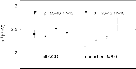
  Figure 13: Comparison of lattice spacings (the quantity plotted is actually the inverse lattice spacing, $a^{-1}$) determined from different physical quantities in quenched and unquenched simulations by the SESAM and T$\chi$L collaborations [36]. $F$ denotes the value determined from the static quark potential and $\rho$ denotes the value determined from the $\rho$-meson mass, while $2S$–$1S$ and $1P$–$1S$ denote values obtained from energy level splittings in $Q\bar{Q}$ bound states using the lattice formulation of nonrelativistic QCD.

• “Quenching”: In most current simulations the matrix elements are evaluated in the “quenched” approximation, in which the effects of virtual quark loops are neglected. For each gluon configuration $\{U_{\mu}(x)\}$, the functional integral over the quark fields in Eq. (56) can be performed formally, giving the determinant of the Dirac operator in the gluon background field corresponding to this configuration. The numerical evaluation of this determinant is possible, but is computationally very expensive, and for this reason the determinant is frequently set equal to its average value, which is equivalent to neglecting virtual quark loops. Gradually, however, unquenched calculations are beginning to be performed, e.g. in fig. 13 we show the lattice spacing obtained by the SESAM and T$\chi$L collaborations from four physical quantities in both quenched and unquenched simulations [36]. In the quenched case there is a spread of results of about $\pm 10\%$, whereas in the unquenched case the spread is smaller (although the errors are still sizeable for some of the quantities used). In the next 3–5 years it should be possible to compute most of the physical quantities discussed below without imposing this approximation.

2.3.2 Lattice Calculations of $B\to\rho,\pi$ Semileptonic Decays:

Having discussed the basics of lattice computations, I now briefly present some results from recent simulations studying $B\to\rho,\pi$ semileptonic decays. I start by making the simple observation that from lattice simulations we can only obtain the form factors for part of the physical phase space for these decays. In order to control discretization errors we require that the three-momenta of the $B$, $\pi$ and $\rho$ mesons be small in lattice units. This implies that we determine the form factors at large values of momentum transfer $q^{2}=(p_{B}-p_{\pi,\rho})^{2}$. Experiments can already reconstruct exclusive semileptonic $b\to u$ decays (see, for example, the review in [21]) and as techniques improve and new facilities begin operation, we can expect to be able to compare the lattice form factor calculations directly with experimental data at large $q^{2}$. A proposal in this direction was made by UKQCD [37] for $\bar{B}^{0}\to\rho^{+}l^{-}\bar{\nu}_{l}$ decays. To get some idea of the precision that might be reached, they parametrize the differential decay rate distribution near $q^{2}_{\mathrm{max}}$ by:

$$\frac{d\Gamma(\bar{B}^{0}\to\rho^{+}l^{-}\bar{\nu}_{l})}{dq^{2}}=10^{-12}\,\frac{G_{F}^{2}|V_{ub}|^{2}}{192\pi^{3}M_{B}^{3}}\,q^{2}\,\lambda^{\frac{1}{2}}(q^{2})\,a^{2}\left(1+b(q^{2}{-}q^{2}_{\mathrm{max}})\right),$$ (65)

where $a$ and $b$ are parameters, and the phase-space factor $\lambda$ is given by $\lambda(q^{2})=(m_{B}^{2}+m_{\rho}^{2}-q^{2})^{2}-4m_{B}^{2}m_{\rho}^{2}$. The constant $a$ plays the role of the IW function evaluated at $\omega=1$ for heavy-to-heavy transitions, but in this case there is no symmetry to determine its value at leading order in the heavy quark effective theory. UKQCD obtain [37]

$$\begin{array}[]{ccc}a=4.6{{\mathop{\raisebox{0.1pt}{\scriptsize$\begin{array}[]{@{}c@{}}+\\ -\end{array}$}}\raisebox{0.1pt}{\scriptsize$\begin{array}[]{@{}r@{}}0.4\\ 0.3\end{array}$}}}\pm 0.6\,\mathrm{Ge\kern-1.00006ptV}&\ \mbox{and}&b=(-8{{\mathop{\raisebox{0.1pt}{\scriptsize$\begin{array}[]{@{}c@{}}+\\ -\end{array}$}}\raisebox{0.1pt}{\scriptsize$\begin{array}[]{@{}r@{}}4\\ 6\end{array}$}}})\times 10^{-2}\,\mathrm{Ge\kern-1.00006ptV}^{2}.\end{array}$$ (66)

The fits are less sensitive to $b$, so it is less well-determined. The result for $a$ incorporates a systematic error dominated by the uncertainty ascribed to discretization errors and would lead to an extraction of $|V_{ub}|$ with less than 10% statistical error and about 12% systematic error from the theoretical input. The prediction for the $d\Gamma/dq^{2}$ distribution based on these numbers is presented in Fig. 14. With sufficient experimental data an accurate lattice result at a single value of $q^{2}$ would be sufficient to fix $|V_{ub}|$.

dΓ/dq2(|Vub|210-12GeV-1) $q^{2}\ (\!\,\mathrm{Ge\kern-1.00006ptV}^{2})$

Figure 14: Differential decay rate as a function of $q^{2}$ for the semileptonic decay $\bar{B}^{0}\to\rho^{+}l^{-}\bar{\nu}_{l}$, taken from [37]. Points are measured lattice data, solid curve is fit from eq. (65) with parameters given in eq. (66). The dashed curves show the variation from the statistical errors in the fit parameters. The vertical dotted line marks the charm endpoint.

In principle, a similar analysis could be applied to the decay $\bar{B}^{0}\to\pi^{+}l^{-}\bar{\nu}_{l}$. However, UKQCD find that the difficulty of performing the chiral extrapolation to a realistically light pion from the unphysical pions used in the simulations makes the results less certain. The $B\to\pi$ decay also has a smaller fraction of events at high $q^{2}$, so it will be more difficult experimentally to extract sufficient data in this region for a detailed comparison.

We would also like to know the full $q^{2}$ dependence of the form factors, which involves a large extrapolation in $q^{2}$ from the high values where lattice calculations produce results, down to $q^{2}=0$. In particular the important radiative decay $\bar{B}\to K^{*}\gamma$ (which is dominated by penguin diagrams in the Standard Model) occurs at $q^{2}=0$, so that existing lattice simulations cannot make a direct calculation of the necessary form factors. Much effort is being devoted to extrapolating the lattice results down to small values of $q^{2}$ exploiting the HQET, light-cone sum-rules [38] and axiomatic properties of quantum field theory. These studies are beyond the scope of these lectures and I refer the students to the review articles [39, 40] for a discussion and references to the original articles.

3 Lecture 3: $K^{0}-\bar{K}^{0}$ and $B^{0}-\bar{B}^{0}$ Mixing

In this lecture I will discuss $K$-$\bar{K}$ and $B$-$\bar{B}$ mixing in turn, and consider the implications of the experimental measurements of these processes for our understanding of the unitarity triangle.

3.1 $K^{0}$-$\bar{K}^{0}$ Mixing, $\epsilon_{K}$ and $\epsilon^{\prime}/\epsilon$

The process of $K^{0}$-$\bar{K}^{0}$ mixing appears in the Standard Model at one-loop level through the box-diagrams of fig. 5 (with the $b$-quark replaced by the $s$-quark), together with possible long-distance contributions. The $CP$-eigenstates ($K_{1}$ and $K_{2}$) are linear combinations of the two strong-interaction eigenstates :

$$|K_{1}\rangle=\frac{1}{\sqrt{2}}\,(|K^{0}\rangle+|\bar{K}^{0}\rangle)\hskip 50.58878ptCP|K_{1}\rangle=|K_{1}\rangle$$ (67)

and

$$|K_{2}\rangle=\frac{1}{\sqrt{2}}\,(|K^{0}\rangle-|\bar{K}^{0}\rangle)\hskip 50.58878ptCP|K_{2}\rangle=-|K_{2}\rangle\ .$$ (68)

Because of the complex phase in the CKM-matrix, the physical states (the mass eigenstates) differ from $|K_{1}\rangle$ and $|K_{2}\rangle$ by a small admixture of the other state:

$$|K_{S}\rangle=\frac{|K_{1}\rangle+\bar{\epsilon}\,|K_{2}\rangle}{(1+|\bar{\epsilon}|^{2})^{\frac{1}{2}}}\ \ \ \textrm{and}\ \ \ |K_{L}\rangle=\frac{|K_{2}\rangle+\bar{\epsilon}\,|K_{1}\rangle}{(1+|\bar{\epsilon}|^{2})^{\frac{1}{2}}}\ ,$$ (69)

(the parameter $\bar{\epsilon}$ depends on the phase convention chosen for $|K^{0}\rangle$ and $|\bar{K}^{0}\rangle$).

For exclusive decays of $K$-mesons (which have angular momentum zero) into two or three pion states, the two pion states are $CP$-even and the three-pion states are $CP$-odd. This implies that the dominant decays are:

$$K_{S}\to\pi\pi\ \ \ \textrm{and}\ \ \ K_{L}\to 3\pi\ ,$$ (70)

which is the reason why $K_{L}$ is much longer lived than $K_{S}$ ($L$ and $S$ stand for long and short respectively). $K_{L}$ and $K_{S}$ are not $CP$-eigenstates, however, and the decay $K_{L}\to 2\pi$ may occur as a result of the small component of $|K_{1}\rangle$ in $|K_{L}\rangle$, and similarly the decay $K_{S}\to 3\pi$ may occur because of the small component of $|K_{2}\rangle$ in $|K_{S}\rangle$. Such $CP$-violating decays which occur due to the fact that the mass eigenstates are not $CP$-eigenstates are called indirect $CP$-violating decays. As mentioned above, the parameter $\bar{\epsilon}$ depends on the convention used to define the phases of the states. A measure of the strength of indirect $CP$-violation is given by the physical parameter $\epsilon_{K}$ defined by the ratio:

$$\epsilon_{K}\equiv\frac{A\left(K_{L}\to(\pi\pi)_{I=0}\right)}{A\left(K_{S}\to(\pi\pi)_{I=0}\right)}=(2.280\pm 0.013)\,10^{-3}\,e^{i\frac{\pi}{4}}\ ,$$ (71)

where $A$ represents the amplitude for the corresponding process and $I=0$ implies that the two pions are in an isospin 0 state. The numerical value in eq. (71) is the empirical result.

Directly $CP$-violating decays are those in which a $CP$-even (-odd) state decays into a $CP$-odd (-even) one:

$$K_{L}\ \ \propto\ \ K_{2}\ \ +\ \ \bar{\epsilon}K_{1}\ .$$ (72)

Consider the possible quark subprocesses contributing to $K\to\pi\pi$ decays shown in fig. 15. The diagrams in fig. 15(b) and (c) are purely real, whereas that of fig. 15(a) is complex. The two pions in the final state can have total isospin $I=0$ or 2; $I=1$ is not possible by Bose symmetry. The final states in the diagrams of fig. 15(a) and (b) clearly have $I=0$, whereas that in the diagram of fig. 15(c) can have either $I=0$ or $I=2$. Thus direct $CP$-violation in kaon decays manifests itself as a non-zero relative phase between the $I=0$ and $I=2$ amplitudes.

Figure 15: Three subprocesses contributing to $K\to\pi\pi$ decays.

Of course the gluonic corrections to the diagrams in fig. 15 generate strong phases, which we denote by $\delta_{0,2}$, where the suffix $0$ or $2$ represents the isospin of the final state. These phases are independent of the form of the weak Hamiltonian. Using the Clebsch-Gordan coefficients for the combination of two isospin 1 pions we write:

$$A(K^{0}\to\pi^{+}\pi^{-}) = \sqrt{\frac{2}{3}}\,A_{0}\,e^{i\delta_{0}}+\sqrt{\frac{1}{3}}\,A_{2}\,e^{i\delta_{2}}$$ (73)

$$A(K^{0}\to\pi^{0}\pi^{0}) = \sqrt{\frac{2}{3}}\,A_{0}\,e^{i\delta_{0}}-2\sqrt{\frac{1}{3}}\,A_{2}\,e^{i\delta_{2}}\ .$$ (74)

The parameter $\epsilon^{\prime}$, which is used as a measure of direct $CP$-violation in kaon decays, is defined by:

$$\epsilon^{\prime}=\frac{\omega}{\sqrt{2}}\,e^{i\phi}\,\left(\frac{\textrm{Im}\,A_{2}}{\textrm{Re}\,A_{2}}-\frac{\textrm{Im}\,A_{0}}{\textrm{Re}\,A_{0}}\right)\ ,$$ (75)

where 

$$\omega\equiv\frac{\textrm{Re}\,A_{2}}{\textrm{Re}\,A_{0}}\ \ \ \textrm{and}\ \ \ \phi=\frac{\pi}{2}+\delta_{2}-\delta_{0}\simeq\frac{\pi}{4}\ .$$ (76)

Experimentally the two parameters $\epsilon_{K}$ (which, following standard conventions I rename from now on as $\epsilon$, $\epsilon\equiv\epsilon_{K}$) and $\epsilon^{\prime}$ can be determined by measuring the ratios:

$$\eta_{00} \equiv \frac{A(K_{L}\to\pi^{0}\pi^{0})}{A(K_{S}\to\pi^{0}\pi^{0})}\,\simeq\ \epsilon-2\epsilon^{\prime}$$ (77)

$$\eta_{+-} \equiv \frac{A(K_{L}\to\pi^{+}\pi^{-})}{A(K_{S}\to\pi^{+}\pi^{-})}\,\simeq\ \epsilon+\epsilon^{\prime}\ .$$ (78)

Direct $CP$-violation is found to be considerable smaller than indirect violation. By measuring the decays and using

$$\left|\frac{\eta_{00}}{\eta_{+-}}\right|^{2}\simeq 1\,-\,6\,\textrm{Re}\,\left(\frac{\epsilon^{\prime}}{\epsilon}\right)\ +\cdots\ ,$$ (79)

the NA31 [41] and E371 [42] experiments find $(23\pm 7)\,10^{-4}$ and $(7.4\pm 5.9)\,10^{-4}$ respectively for $\epsilon^{\prime}/\epsilon$. The Particle Data Group [7] summarises these results as:

$$\epsilon^{\prime}/\epsilon=(1.5\pm 0.8)\,10^{-3}\ .$$ (80)

We will have to wait for the results of the current generation of experiments, which will have a sensitivity of $O(10^{-4})$, to confirm or deny whether the value is indeed different from zero.

3.1.1 Determination of $\epsilon$

In this subsection I discuss the theoretical determination of $\epsilon$, following the discussion and notation in the review article by Buras and Fleischer [1]. We need to know the matrix element:

$$\langle\bar{K}^{0}\,|\,\mathcal{H}^{\Delta S=2}_{\scriptstyle{eff}}\,|\,K^{0}\rangle\ ,$$ (81)

where we write the effective Hamiltonian in the form:

$$\mathcal{H}^{\Delta S=2}_{\scriptstyle{eff}} = \frac{G_{F}^{2}}{16\pi^{2}}M_{W}^{2}\left[\lambda_{c}^{2}\eta_{1}S_{0}(x_{c})\ +\ \lambda_{t}^{2}\eta_{2}S_{0}(x_{t})+2\lambda_{c}\lambda_{t}\eta_{3}S_{0}(x_{c},x_{t})\right]$$ (82)

$$\mbox{\ \ \ }\times\left[\alpha_{s}^{(3)}(\mu)\right]^{-\frac{2}{9}}\,\left[1+\frac{\alpha_{s}^{(3)}(\mu)}{4\pi}J_{3}\right]\,O^{\Delta S=2}(\mu)\ +\ \textrm{h.c.}\ ,$$

the renormalization scale $\mu$ is chosen to be much smaller than $m_{c}$, $x_{i}=m_{i}^{2}/M_{W}^{2}$ and $\lambda_{i}=V_{id}V_{is}^{*}$ (the dependence on $\lambda_{u}$ is eliminated by unitarity, $x_{u}=0$). The non-perturbative QCD effects for $K^{0}$-$\bar{K}^{0}$ mixing are all contained in the matrix elements of the single local composite operator

$$O^{\Delta S=2}(\mu)=\bar{s}\gamma^{\mu}(1-\gamma^{5})d\ \bar{s}\gamma_{\mu}(1-\gamma^{5})d\ ,$$ (83)

the remaining terms in eq. (82) can be calculated in perturbation theory. The $S_{0}$’s are the expressions for the box-diagrams without QCD corrections:

$$S_{0}(x) = \frac{4x-11x^{2}+x^{3}}{4(1-x)^{2}}\,-\,\frac{3x^{3}\ln(x)}{2(1-x)^{3}}$$ (84)

$$S_{0}(x_{c},x_{t}) = x_{c}\left[\ln\left(\frac{x_{t}}{x_{c}}\right)-\frac{3x_{t}}{4(1-x_{t})}-\frac{3x_{t}^{2}\ln(x_{t})}{4(1-x_{t})^{2}}\right]+\cdots\ .$$ (85)

$\eta_{1},\eta_{2}$ and $\eta_{3}$ are mass-dependent short-distance QCD factors, at NLO (next-to leading order)

$$\eta_{1}=1.38\pm 0.20\ \ \ \eta_{2}=0.57\pm 0.01\ \ \textrm{and}\ \ \eta_{3}=0.47\pm 0.04\ ,$$ (86)

where the errors reflect the uncertainty in $\Lambda_{\mathrm{QCD}}$ and the quark masses. The remaining factors in eq. (82) are short-distance QCD effects, whose $\mu$-dependence cancels that in the operator $O^{\Delta S=2}$ (in the NDR-renormalization scheme $J_{3}$=1.895).

As mentioned above, all the non-perturbative QCD corrections are contained in the matrix elements of $O^{\Delta S=2}$. It is conventional to introduce the $B_{K}$ parameter by the definition:

$$\langle\bar{K}^{0}\,|\,\bar{s}\gamma^{\mu}(1-\gamma^{5})d\ \bar{s}\gamma_{\mu}(1-\gamma^{5})d\,|K^{0}\rangle\equiv\frac{8}{3}m_{K}^{2}f_{K}^{2}B_{K}(\mu)\ .$$ (87)

The motivation for introducing the parameter $B_{K}$ in this way comes from the vacuum saturation approximation (in which $B_{K}=1$), but there is no loss of generality in this definition. $B_{K}(\mu)$ depends on the renormalization scale, and it is convenient to introduce an (almost) renormalization group invariant $B_{K}$ by:

$$B_{K}=B_{K}(\mu)\left[\alpha_{s}^{(3)}(\mu)\right]^{-\frac{2}{9}}\,\left[1+\frac{\alpha_{s}^{(3)}(\mu)}{4\pi}J_{3}\right]\ .$$ (88)

The weakest link in the theoretical calculation of $\epsilon$ is the evaluation of $B_{K}$. Many lattice computations have been performed, and a recent compilation of results gave $B_{K}=0.90\pm 0.06$ [43]. A calculation based on the $1/N$ approximation gave $B_{K}=0.70\pm 0.10$ [44]. Buras and Fleischer perform their analysis with

$$B_{K}=0.75\pm 0.15\ .$$ (89)

$\epsilon$ is given in terms of the quantities introduced above by

$$\epsilon=C_{\epsilon}\,B_{K}\,\textrm{Im}\,\lambda_{t}\left\{\textrm{Re}\,\lambda_{c}\left[\eta_{1}S_{0}(x_{c})-\eta_{3}S_{0}(x_{c},x_{t})\right]-\textrm{Re}\,\lambda_{t}\,\eta_{2}S_{0}(x_{t})\right\}\,e^{i\frac{\pi}{4}}\ ,$$ (90)

where

$$C_{\epsilon}=\frac{G_{F}^{2}f_{K}^{2}m_{K}M_{W}^{2}}{6\sqrt{2}\pi^{2}(\Delta M_{K})}=3.78\cdot 10^{4}$$ (91)

and the mass difference $\Delta M_{K}=M_{K_{L}}-M_{K_{S}}$.

We obtain information about the unitarity triangle by comparing the theoretical prediction with the experimentally measured value of $\epsilon$. In terms of $\bar{\eta}$ and $\bar{\rho}$ the prediction is the hyperbola

$$\bar{\eta}\left[(1-\bar{\rho})A^{2}\eta_{2}S_{0}(x_{t})+P_{0}\right]\,A^{2}\,B_{K}\,=\,0.226\ ,$$ (92)

where $P_{0}=0.31\pm 0.02$. This is illustrated in fig. 16.

Figure 16: A precise determination of $\epsilon$ would fix the vertex $A$ to lie on a a hyperbola (schematically represented by the solid curve).

3.1.2 The $\Delta I=1/2$ Rule and $\epsilon^{\prime}/\epsilon$

In this subsection I briefly review the elements in the theoretical predictions for $\epsilon^{\prime}/\epsilon$ and related quantities. I start by rewriting eq. (75) in the form:

$$\epsilon^{\prime}=-\frac{\omega}{\sqrt{2}}\,\xi\,(1-\Omega)\,e^{i\phi}\ ,$$ (93)

where

$$\omega=\frac{\textrm{Re}\,A_{2}}{\textrm{Re}\,A_{0}}\,,\ \ \xi=\frac{\textrm{Im}\,A_{0}}{\textrm{Re}\,A_{0}}\,,\ \ \Omega=\frac{1}{\omega}\frac{\textrm{Im}\,A_{2}}{\textrm{Im}\,A_{0}}\ \ \textrm{and}\ \ \phi=\frac{\pi}{2}+\delta_{2}-\delta_{0}\simeq\frac{\pi}{4}\ .$$ (94)

Even after about 40 years, we still do not understand theoretically the $\Delta I=1/2$ rule, i.e. the empirical observation that $\omega\simeq 1/22$. The rate for transitions in which the isospin changes by 1/2 ($\Delta I=1/2$ transitions) is enhanced by a factor of about 450 over those in which it changes by 3/2 ($\Delta I=3/2$ transitions). There is a relatively small enhancement of the $\Delta I=1/2$ amplitudes, by a factor of 2-3, due to perturbative effects (i.e. in the calculation of the Wilson coefficient function). The remaining enhancement is assumed to be due to long-distance QCD effects, perhaps because the matrix-elements of penguin operators are large, but this has still to be convincingly demonstrated.

In the recent analyses of $\epsilon^{\prime}/\epsilon$, one combines the experimental values for the real parts of the amplitudes (Re $A_{0}=3.33\cdot 10^{-7}\,$GeV, Re $A_{2}=1.50\cdot 10^{-8}\,$GeV, $\omega=0.045$), with theoretical predictions for the imaginary parts. The effective Hamiltonian for these $\Delta S=1$ transitions takes the form:

$$\mathcal{H}_{eff}(\Delta S=1)=\frac{G_{F}}{\sqrt{2}}\,\sum_{i=1}^{10}\left(z_{i}(\mu)+\tau y_{i}(\mu)\right)\,O_{i}(\mu)\ ,$$ (95)

where $\tau=-V_{td}V^{*}_{ts}/V_{ud}V^{*}_{us}$. There are 10 independent operators in the $\Delta S=1$ effective Hamiltonian, and the major uncertainty is in the values of their matrix elements and in the mass of the strange quark $m_{s}$. The most complete analyses have been performed by Buras et al [45] who find:

$$(-1.2\cdot 10^{-4})<\epsilon^{\prime}/\epsilon<16\cdot 10^{-4}\ \ (I)\ \ ;\ \ \epsilon^{\prime}/\epsilon=(3.6\pm 3.4)\,10^{-4}\ \ (II)\ ,$$ (96)

where $I$ and $II$ refer to two different ways of treating the many uncertainties (more and less conservative respectively), and by the Rome group [46] who find

$$\epsilon^{\prime}/\epsilon=(4.6\pm 3.0)\,10^{-4}\ .$$ (97)

The various contributions to $\epsilon^{\prime}/\epsilon$ have different signs, and there are significant cancellations. For this reason even the expected sign cannot be predicted with full confidence.

I end this subsection with a brief summary of the main points:

• An understanding of the $\Delta I=1/2$ rule would be an important milestone in controlling non-perturbative QCD effects. This is a realistic, but non-trivial, challenge for the lattice community.

• A measurement of a non-zero value for $\epsilon^{\prime}/\epsilon$ would be a very important qualitative step in particle physics; confirming the existence of direct $CP$-violation.

• The uncertainties in the values of the matrix elements, make it difficult to make a precise prediction for $\epsilon^{\prime}/\epsilon$. We expect it to be at the several $\times 10^{-4}$ level, but accidental cancellations between contributions with opposite signs may make it smaller than this. In the coming years, experiments at CERN, FNAL and at Da$\phi$ne will be sensitive to a value of about $10^{-4}$.

3.2 $B^{0}$-$\bar{B}^{0}$ Mixing

In this subsection we consider $B$-$\bar{B}$ mixing, from which we get information about the $V_{td}$ and $V_{ts}$ elements of the CKM-matrix. I start with some general formalism for the mixing of a neutral psudoscalar meson $P^{\,0}$ with its antiparticle $\bar{P}^{\,0}$. I write the wave-function in two-component form:

$$|\psi(t)\rangle=\left(\begin{array}[]{c}a(t)\\ b(t)\end{array}\right)\equiv a(t)\,|P^{0}\rangle+b(t)\,|\bar{P}^{0}\rangle\ .$$ (98)

The time dependence of $|\psi(t)\rangle$ is given by the Schrödinger equation:

$$i\frac{d}{dt}\,|\psi(t)\rangle=\left(M-\frac{i\Gamma}{2}\right)|\psi(t)\rangle\ ,$$ (99)

where $M-i\Gamma/2$ is the $2\times 2$ “mass-matrix”, whose elements are equal to $\langle P_{i}^{0}|\mathcal{H}_{eff}|P_{j}^{0}\rangle/2M_{P}$. Using the optical theorem, the absorbtive part of this matrix comes from real intermediate states:

$$\Gamma_{ij}=\frac{1}{2M_{P}}\sum_{n}\langle P^{\,0}_{i}\,|\mathcal{H}_{W}\,|n\rangle\langle n\,|\mathcal{H}_{W}\,|P^{\,0}_{j}\rangle\,2\pi\,\delta(E_{n}-M_{P})\ .$$ (100)

For $B^{0}$-$\bar{B}^{0}$ mixing, there are no contributions to $\Gamma_{12}$ from intermediate states containing the top quark.

The mass-matrix takes the form

$$M-\frac{i\Gamma}{2}=\left(\begin{array}[]{cc}A&\ \,p^{2}\\ q^{2}&\ \,A\end{array}\right)\ ,$$ (101)

where the diagonal terms are equal by CPT-invariance, and $A$, $p^{2}$ and $q^{2}$ are complex. The eigenvalues of this matrix are $M_{1,2}=A\pm pq$, so that the mass difference between the two physical eigenstates is

$$\Delta M=M_{1}-M_{2}=2pq=2(M_{12}-i\Gamma_{12})^{\frac{1}{2}}(M_{12}^{*}-i\Gamma_{12}^{*})^{\frac{1}{2}}\ .$$ (102)

For the $B$-system, the box diagrams have contributions from $t$-quarks in the loops (see fig. 5). By unitarity these contribute only to the real part of the mass-matrix. The mass behaviour of the box diagrams in fig. 5, and the large value of $V_{tb}$ imply that these contributions dominate and that $|\Gamma_{12}|\ll|M_{12}|$ for $B$-$\bar{B}$ mixing (this is not the case for $K$-$\bar{K}$ mixing). Thus $\Delta M\simeq 2|M_{12}|$, and can be calculated from the box diagrams.

The evaluation of the box diagrams follows similarly to that in the kaon system. The non-perturbative QCD effects are contained in the matrix element of the $\Delta B=2$ operator:

$$O^{\Delta B=2}=\bar{b}\gamma^{\mu}(1-\gamma^{5})d\ \bar{b}\gamma_{\mu}(1-\gamma^{5})d\ ,$$ (103)

and it is also convenient and conventional to introduce the $B_{B}$ parameter analogously to the definition of $B_{K}$ in eq. (87). The theoretical expression for the mass difference is:

$$\Delta M=\frac{G_{F}^{2}}{6\pi^{2}}\,\eta_{B}\,M_{B}\,B_{B}\,f_{B}^{2}\,M_{W}^{2}\,S_{0}(x_{t})\,|V_{td}|^{2}\ ,$$ (104)

where $\eta_{B}$ is a pertubative QCD correction ($\eta_{B}=0.55\pm 0.01$). Throughout this discussion I have been implicitly assuming that we are considering neutral $B_{d}$ mesons, but an analogous discussion holds for the $B_{s}$ system. In the kaon system, all the non-perturbative QCD effects were contained in the parameter $B_{K}$, since the leptonic decay constant $f_{K}$ is a measured quantity. For the $B$-mesons this is not the case, and one is obliged to use model estimates or lattice or sum-rule calclulations for both the decay constants $f_{B}$ and the $B_{B}$-parameters (or of the matrix element of $O^{\Delta B=2}$ itself). For example, in a recent compilation of lattice results we obtained [39]:

$$f_{B_{d}}=(170\pm 35)\,\mathrm{Ge\kern-1.00006ptV},\ \ f_{B_{s}}=(195\pm 35)\,\mathrm{Ge\kern-1.00006ptV},\ \ B_{B_{d}}=1.4(1),$$ (105)

and

$$\xi\equiv\frac{f_{B_{s}}\sqrt{B_{B_{s}}}}{f_{B_{d}}\sqrt{B_{B_{d}}}}=1.14(8)\ .$$ (106)

Combining all the elements one obtains:

$$\Delta M_{B_{d}} = 0.50\,\textrm{ps}^{-1}\,\left[\frac{f_{B_{d}}\sqrt{B_{B_{d}}}}{200\,\mathrm{Me\kern-1.00006ptV}}\right]^{2}\,\left(\frac{\bar{m}_{t}(m_{t})}{170\,\mathrm{Ge\kern-1.00006ptV}}\right)^{1.52}\,\frac{|V_{td}|}{0.0088}\ \frac{\eta_{B}}{0.55}$$ (107)

$$\Delta M_{B_{s}} = 15.1\,\textrm{ps}^{-1}\,\left[\frac{f_{B_{s}}\sqrt{B_{B_{s}}}}{240\,\mathrm{Me\kern-1.00006ptV}}\right]^{2}\,\left(\frac{\bar{m}_{t}(m_{t})}{170\,\mathrm{Ge\kern-1.00006ptV}}\right)^{1.52}\,\frac{|V_{ts}|}{0.040}\ \frac{\eta_{B}}{0.55}\ .$$ (108)

The mass difference $\Delta M$ is a measure of the oscillation frequency to change from a $B^{0}$ to a $\bar{B}^{0}$ and vice-versa. Imagine that we start with a $B^{0}$ at time $t=0$, then the propabilities that we have a $B^{0}$ or $\bar{B}^{0}$ at a later time $t$ are $\exp(-\Gamma t)\cos^{2}(\Delta M\,t/2)$ and $\exp(-\Gamma t)\sin^{2}(\Delta M\,t/2)$ respectively. Defining $P(B^{0})$ and $P(\bar{B}^{0})$ to be the probabilities (obtained by integrating over time) that when the meson decays it is a $B$ or $\bar{B}$ respectively, we obtain

$$P(B^{0})=\frac{1}{2}\,\left[\frac{1}{\Gamma}+\frac{\Gamma}{\Gamma^{2}+(\Delta M)^{2}}\right]\ \ \textrm{and}\ \ P(\bar{B}^{0})=\frac{1}{2}\,\left[\frac{1}{\Gamma}-\frac{\Gamma}{\Gamma^{2}+(\Delta M)^{2}}\right]\ .$$ (109)

The ratio of these integrated probabilities is given by

$$r\equiv\frac{P(B^{0})}{P(\bar{B}^{0})}\ =\ \frac{x^{2}}{2+x^{2}}\ ,$$ (110)

where $x=\Delta M/\Gamma$. The 1996 Particle Data Group review quotes:

$$\Delta M_{B_{d}}=(0.474\pm 0.031)\,\textrm{ps}^{-1}\ \ \textrm{and}\ \ x_{d}=0.73\pm 0.05\ ,$$ (111)

in agreement with theoretical expectations and

$$\Delta M_{B_{s}}>5.9\,\textrm{ps}^{-1}\ \ \textrm{and}\ \ x_{s}>9.5\ \ \textrm{at }95\%\ \textrm{CL}\ .$$ (112)

The oscillation in the $B_{s}$ system are too rapid for observation in experiments which have been performed up to date.

What do these measurements imply for the determination of the position of the unitarity triangle? In principle a measurement of $\Delta M_{B_{d}}$ allows for a determination of the $V_{td}$ element of the CKM matrix. The side $BA$ of the unitarity triangle is given by:

$$\frac{|V_{td}V_{tb}^{*}|}{|V_{cd}V_{cb}^{*}|}=\frac{1}{\lambda}\frac{|V_{td}|}{|V_{cb}|}=\sqrt{(1-\bar{\rho})^{2}+\bar{\eta}^{2}}\ ,$$ (113)

so that a measurement of $V_{td}$ (assuming knowledge of $V_{cb}$) would imply that the locus of possible positions of the vertex $A$ lies on a given circle centred on $B$, see fig. 17.

Figure 17: A precise determination of $|V_{td}/V_{cb}|$ from studies of $B-\bar{B}$ mixing would fix the vertex $A$ to lie on a circle centered on the vertex $B$ (schematically represented by the solid curve).

4 Lecture 4: CP-Violation in $B$-Decays and Inclusive $B$-Decays

In this final lecture I will consider two topics in $B$-physics, $CP$-violation (and mixing-induced $CP$-violation, in particular) and the application of the heavy quark expansion to inclusive decays (and to beauty-lifetimes and the semileptonic branching ratio, in particular). I will also make some brief remarks about how difficult it is to make predictions for exclusive nonleptonic decays.

4.1 $CP$-Violation in $B$-Decays

Measurements of $CP$-asymmetries in neutral $B$-meson decays into $CP$-eigenstates will allow us to address 3 fundamental questions:

1. Is the phase in the CKM matrix the only source of $CP$-violation?

2. What are the precise values of the CKM parameters? We shall see that the principal systematic errors, particularly those due to hadronic uncertainties, are reduced significantly in some cases.

3. Is there new physics in the quark-sector?

A particularly important class of decays of neutral $B$-meson systems, are mixing induced $CP$-violating decays (these are not possible in decays of charged $B$-mesons). I now briefly review this important topic, for which we need to return to the formalism introduced in the discussion of $B$-$\bar{B}$ mixing in subsec. 3.2 above. The two neutral mass-eigenstates are given by

$$|B_{L}\rangle=\frac{1}{\sqrt{p^{2}+q^{2}}}\,\left(p\,|B^{0}\rangle+q\,|\bar{B}^{0}\rangle\right)\ \ \textrm{and}\ \ |B_{H}\rangle=\frac{1}{\sqrt{p^{2}+q^{2}}}\,\left(p\,|B^{0}\rangle-q\,|\bar{B}^{0}\rangle\right)\ .$$ (114)

Starting with a $B^{0}$ meson at time $t=0$, its subsequent evolution is governed by the Schrödinger equation (99):

$$|B^{0}_{\mathrm{phys}}(t)\rangle=g_{+}(t)\,|B^{0}\rangle+\left(\frac{q}{p}\right)g_{-}(t)|\bar{B}^{0}\rangle\ ,$$ (115)

where

$$g_{+}(t) = \exp\left[-\frac{\Gamma t}{2}\right]\,\exp[-iMt]\,\cos\left(\frac{\Delta M\,t}{2}\right)\ ,$$ (116)

$$g_{-}(t) = \exp\left[-\frac{\Gamma t}{2}\right]\,\exp[-iMt]\,i\sin\left(\frac{\Delta M\,t}{2}\right)\ ,$$ (117)

and $M=(M_{H}+M_{L})/2$ .

4.1.1 Decays of Neutral $B$-Mesons into $CP$-Eigenstates

Let $f_{CP}$ be a $CP$-eigenstate and $A,\bar{A}$ be the amplitudes

$$A\equiv\langle f_{CP}|\mathcal{H}|B^{0}\rangle\ \ \textrm{and}\ \ \bar{A}\equiv\langle f_{CP}|\mathcal{H}|\bar{B}^{0}\rangle\ .$$ (118)

Defining

$$\lambda\equiv\frac{q}{p}\,\frac{\bar{A}}{A}$$ (119)

we have

$$\langle f_{CP}\,|\,\mathcal{H}\,|\,B^{0}_{\mathrm{phys}}\rangle=A\,[g_{+}(t)\,+\,\lambda\,g_{-}(t)]\ \ \ \textrm{and}\ \ \ \langle f_{CP}\,|\,\mathcal{H}\,|\,\bar{B}^{0}_{\mathrm{phys}}\rangle=A\,\frac{p}{q}\,[g_{-}(t)\,+\,\lambda\,g_{+}(t)]\ .$$ (120)

The time-dependent rates for initially pure $B^{0}$ or $\bar{B}^{0}$ states to decay into the $CP$-eigenstate $f_{CP}$ at time $t$ are given by:

$$\Gamma(B^{0}_{\mathrm{phys}}(t)\to f_{CP}) = |A|^{2}\,e^{-\Gamma t}\left[\frac{1+|\lambda|^{2}}{2}\,+\,\frac{1-|\lambda|^{2}}{2}\cos(\Delta M\,t)-\textrm{Im}\,\lambda\,\sin(\Delta M\,t)\right]$$ (121)

$$\Gamma(\bar{B}^{0}_{\mathrm{phys}}(t)\to f_{CP}) = |A|^{2}\,e^{-\Gamma t}\left[\frac{1-|\lambda|^{2}}{2}\,+\,\frac{1-|\lambda|^{2}}{2}\cos(\Delta M\,t)+\textrm{Im}\,\lambda\,\sin(\Delta M\,t)\right]\ .$$ (122)

The time-dependent asymmetry is defined as:

$$\mathcal{A}_{f_{CP}}(t) \equiv \frac{\Gamma(B^{0}_{\mathrm{phys}}(t)\to f_{CP})-\Gamma(\bar{B}^{0}_{\mathrm{phys}}(t)\to f_{CP})}{\Gamma(B^{0}_{\mathrm{phys}}(t)\to f_{CP})+\Gamma(\bar{B}^{0}_{\mathrm{phys}}(t)\to f_{CP})}$$ (123)

$$= \frac{(1-|\lambda|^{2})\cos(\Delta M\,t)-2\textrm{Im}\,\lambda\,\sin(\Delta M\,t)}{1+|\lambda|^{2}}\ .$$ (124)

If, as is the case in some important applications, $|q/p|=1$ (which is the case if $\Delta\Gamma<<\Delta M$) and $|\bar{A}/A|=1$ (examples of this will be presented below), then $|\lambda|=1$ and the first term on the right-hand side of eq.(124) vanishes.

The form of the amplitudes $A$ and $\bar{A}$ is:

$$A=\sum_{i}\,A_{i}\,e^{i\delta_{i}}\,e^{i\phi_{i}}\ \ \ \textrm{and}\ \ \ \bar{A}=\sum_{i}\,A_{i}\,e^{i\delta_{i}}\,e^{-i\phi_{i}}$$ (125)

where the sum is over all the contributions to the process, the $A_{i}$ are real, $\delta_{i}$ are the strong phases and the $\phi_{i}$ are the phases from the CKM matrix. In the most favourable situation, all the contributions have a single CKM phase ($\phi_{D}$ say) and $\bar{A}/A=\exp(-2i\phi_{D})$. Under the assumption we are making that $\Gamma_{12}<<M_{12}$, $q/p=\sqrt{M_{12}^{*}/M_{12}}\equiv\exp(-2i\phi_{M})$, and $\lambda=\exp(-2i(\phi_{D}+\phi_{M}))$. Thus

$$\textrm{Im}\,\lambda=-\sin(2(\phi_{D}+\phi_{M}))\ .$$ (126)

From the box diagrams of fig. 5 we obtain:

$$\left(\frac{q}{p}\right)_{B_{d}}=\frac{V_{td}V_{tb}^{*}}{V^{*}_{td}V_{tb}}\ \ \ \textrm{and}\ \ \ \left(\frac{q}{p}\right)_{B_{s}}=\frac{V_{ts}V_{tb}^{*}}{V^{*}_{ts}V_{tb}}\ .$$ (127)

To illustrate the above discussion let us consider three processes in which the $b$-quark decays through the subprocess $b\to d_{j}u_{i}\bar{u}_{i}$. The corresponding tree-level diagram is

$$\mbox{\begin{picture}(80.0,50.0)(80.0,20.0) \put(0.0,0.0){} \put(0.0,0.0){} \put(0.0,0.0){} \put(0.0,0.0){} \raise 45.0pt\hbox to0.0pt{\kern 5.0pt\makebox(0.0,0.0)[r]{$b$}\hss} \ignorespaces \raise 45.0pt\hbox to0.0pt{\kern 85.0pt\makebox(0.0,0.0)[l]{$u_{i}$}\hss} \ignorespaces \raise 25.0pt\hbox to0.0pt{\kern 110.0pt\makebox(0.0,0.0)[l]{$d_{j}$}\hss} \ignorespaces \raise 5.0pt\hbox to0.0pt{\kern 110.0pt\makebox(0.0,0.0)[l]{$\bar{u}_{i}$}\hss} \ignorespaces \end{picture}}\textrm{for which}\ \ \ \ \frac{\bar{A}}{A}=\frac{V_{ib}V_{ij}^{*}}{V_{ib}^{*}V_{ij}}\ .$$ (128)

$\mathbf{B_{d}\to J/\Psi\,K_{S}:}$

In this case

$$\lambda(B\to J/\Psi K_{S})=\frac{V_{td}V_{tb}^{*}}{V_{td}^{*}V_{tb}}\ \frac{V_{cs}V_{cd}^{*}}{V_{cs}^{*}V_{cd}}\ \frac{V_{cb}V_{cs}^{*}}{V_{cb}^{*}V_{cs}}\ =-\sin(2\beta)\ .$$ (129)

The first factor in eq. (129) is the factor $(q/p)_{B_{d}}$ in eq. (127), the third factor is the analogous one for the final state kaon, and the second factor is $\bar{A}/A$ as in eq. (128) with $u_{i}=c$ and $b_{j}=s$. We recall from the discussion of the first lecture that the angle

$$\beta=\arg\left(-\frac{V_{cd}V_{cb}^{*}}{V_{td}V_{tb}^{*}}\right)\ .$$ (130)

There is also a small penguin contribution to this process, due to the subprocess:

which is proportional to $V_{tb}V_{ts}^{*}$, whose phase is, to a very good approximation, equal to that of $V_{cb}V_{cs}^{*}$. Thus hadronic uncertainties are negligible in the determination of the angle $\beta$ from this process, and for this reason we can consider it a gold-plated one. This is an (almost) ideal situation.

$\mathbf{B_{d}\to\pi^{+}\pi^{-}:}$

For this process, in the notation of eq. (128), we have $u_{i}=u$ and $d_{j}=d$, so that

$$\frac{\bar{A}}{A}=\frac{V_{ub}V_{ud}^{*}}{V_{ub}V_{ud}^{*}}$$ (131)

and Im $\lambda=\sin(2\alpha)$, where from the first lecture we recall that

$$\alpha=\arg\left(-\frac{V_{td}V_{tb}^{*}}{V_{ud}V_{ub}^{*}}\right)\ .$$ (132)

In this case there is also a small penguin contribution, which is proportional to $V_{td}^{*}V_{tb}$, which has a different phase from the tree diagram. This implies that the hadronic uncertainites are greater than for the process $B_{d}\to J/\Psi K_{S}$, although they are still reasonably small (and can be reduced further using isospin analysis).

$\mathbf{B_{s}\to\rho^{0}K_{S}:}$

For this process in the notation of eq. (128), we have $u_{i}=u$ and $d_{j}=d$ again, so that

$$\lambda(B_{s}\to\rho K_{S})=\frac{V_{ts}V_{tb}^{*}}{V_{ts}^{*}V_{tb}}\ \frac{V_{ub}V_{ud}^{*}}{V_{ub}^{*}V_{ud}}\ \frac{V_{cd}V_{cs}^{*}}{V_{cd}^{*}V_{cs}}\ .$$ (133)

Using the unitarity relations and the fact that

$$\gamma=\arg\left(-\frac{V_{ud}V_{ub}^{*}}{V_{cd}V_{cb}^{*}}\right)\ ,$$ (134)

we find that Im $\lambda=-\sin(2\gamma)$.

Although this process is frequently proposed as a potential way of measuring the angle $\gamma$, the penguin contributions are relatively large and Buras and Fleischer stress that it is a wrong way [1]. It has been suggested that it might be possible to use combinations of $B\to DK$ amplitudes to determine the angle $\gamma$ [47]. This is illustrated in fig. 18, where $|D^{0}_{+}\rangle=1/\sqrt{2}(\,|D^{0}\rangle+|\bar{D}^{0}\rangle\,)$, but clearly a measurement of all the amplitudes is a huge experimental challenge.

Figure 18: Six amplitudes from which the angle $\gamma$ can (in principle at least) be determined.

The exciting experimental and theoretical program of research into mixing induced $CP$-asymetries will continue at the (near) future $B$-factories and dedicated $B$-experiments.

4.1.2 $CP$-Violation in Charged $B$-Decays

Observation of $CP$-violation in decays of charged $B$-mesons would demonstrate the existence of direct $CP$-violation, but the hadronic uncertainties make it unlikely that they can be used to determine the parameters of the unitarity triangle with the required precision. Since we need an interference between different contributions to the amplitude, we write the amplitudes in the form:

$$A(B^{-}\to f)=V_{1}\,A_{1}\,e^{i\delta_{1}}+V_{2}\,A_{2}\,e^{i\delta_{2}}\ \ \ \textrm{and}\ \ \ A(B^{+}\to\bar{f})=V_{1}^{*}\,A_{1}\,e^{i\delta_{1}}+V_{2}^{*}\,A_{2}\,e^{i\delta_{2}}\ ,$$ (135)

where I have exhibited two contributions to each amplitude, $V_{1,2}$ are CKM-matrix elements and the $\delta_{1,2}$ are strong interaction phases. For example in the process $B^{+}\to\pi^{0}K^{+}$ the interference is between curent-current and penguin contributions, and in the decay $B^{+}\to\bar{K}^{0}K^{+}$ it is between penguin diagrams with internal $u$ and $c$ quarks.

The $CP$-violating asymmetry is now defined by

$$\mathcal{A}_{CP}\equiv\frac{\Gamma(B^{+}\to\bar{f}){-}\Gamma(B^{-}\to f)}{\Gamma(B^{+}\to\bar{f})+\Gamma(B^{-}\to f)}=\frac{2\,\textrm{Im}\,(V_{1}V_{2}^{*})\,\sin(\delta_{1}{-}\delta_{2})\,A_{1}A_{2}}{|V_{1}|^{2}A_{1}^{2}+|V_{2}|^{2}A_{2}^{2}+2\textrm{Re}\,(V_{1}V_{2}^{*})\cos(\delta_{1}{-}\delta_{2})\,A_{1}A_{2}}\ ,$$ (136)

from which we see that in order to have a non-zero asymmetry we require both Im $(V_{1}V_{2}^{*})$ and $\sin(\delta_{1}-\delta_{2})$ to be non-zero. The strong interaction phases are very difficult to quantify, so it is hard to use measurements of these $CP$-asymetries to determine the CKM matrix elements.

4.2 Inclusive Nonleptonic Decays of Beauty Hadrons

In this subsection I discuss inclusive nonleptonic decays of beauty hadrons in general, and two very interesting phenomenological problems in particular the lifetimes of the hadrons and their semileptonic branching ratios. The discussion will use the formalism of Bigi et al.(see ref. [48] and references therein), developed and used by them and many other groups, in which inclusive quantities are expanded in inverse powers of the mass of the heavy quark, e.g.

$$\Gamma(H_{b})=\frac{G_{F}^{2}m_{b}^{5}|V_{cb}|^{2}}{192\pi^{3}}\left\{c_{3}\left(1+\frac{\lambda_{1}+3\lambda_{2}}{2m_{b}^{2}}\right)+c_{5}\frac{\lambda_{2}}{m_{b}^{2}}+O\left(\frac{1}{m_{b}^{3}}\right)\right\}\ ,$$ (137)

where $\Gamma$ is the full or partial width of a beauty hadron $H_{b}$, $c_{3,5}$ are coefficients which can be computed in perturbation theory (the coefficient functions obtained when matching QCD onto the HQET) and $\lambda_{1,2}$ are the matrix elements of the kinetic energy and chromomagnetic operators respectively:

$$\lambda_{1}(B)=\frac{1}{2m_{H_{b}}}\langle H_{b}|\,\bar{h}(i\mathbf{D})^{2}h\,|H_{b}\rangle\ \ \ \ \textrm{and}\ \ \ \ \lambda_{2}=\frac{1}{3}\frac{\langle H_{b}|\bar{h}\frac{1}{2}\sigma_{ij}G^{ij}h|H_{b}\rangle}{2m_{H_{b}}}\ ,$$ (138)

and $h$ is the field of the heavy (static) quark. An important feature of the general expression in eq. (137) is the absence of terms of $O(1/m_{b})$, which is a consequence of the absence of any operators of dimension 4 which can appear in the corresponding OPE [49].

I will not discuss the derivation of the expansion in eq. (137) in detail. One starts, similarly to the derivation of the OPE for moments of deep-inelastic structure functions, by using the optical theorem which states that the width is given by the imaginary part of the forward elastic amplitude. In this case this amplitude has two insertions of the weak Hamiltonian. Since the $b$-quark is heavy and decays into lighter states, the separation of these two insertions is small, and eq. (137) is the corresponding short distance expansion (for the structure functions it is a light-cone expansion). We now apply this expansion to a study of beauty lifetimes and the semileptonic brabching ratio.

4.2.1 Beauty Lifetimes

Using the expression in eq. (137) for the widths, one readily finds the following results for the ratios of lifetimes:

$$\frac{\tau(B^{-})}{\tau(B^{0})} = 1+O\left(\frac{1}{m_{b}^{3}}\right)$$ (139)

$$\frac{\tau(\Lambda_{b})}{\tau(B^{0})} = 1+\frac{\mu_{\pi}^{2}(\Lambda_{b})-\mu_{\pi}^{2}(B)}{2m_{b}^{2}}+c_{G}\frac{\mu_{G}^{2}(\Lambda_{b})-\mu_{G}^{2}(B)}{m_{b}^{2}}+O\left(\frac{1}{m_{b}^{3}}\right)$$ (140)

$$= (0.98\pm 0.01)+O\left(\frac{1}{m_{b}^{3}}\right)\ ,$$

where $\mu_{\pi}^{2}=-\lambda_{1}$ and $\mu_{G}^{2}=3\lambda_{2}$. In order to obtain the result in eq.(140), one needs to know the difference of the kinetic energies of the $b$-quark in the baryon and meson. To leading order in the heavy quark expansion we have:

$$\mu_{\pi}^{2}(\Lambda_{b})-\mu_{\pi}^{2}(B)=-\frac{M_{B}M_{D}}{2}\left(\frac{M_{\Lambda_{b}}-M_{\Lambda_{c}}}{M_{B}-M_{D}}-\frac{3}{4}\frac{M_{B^{*}}-M_{D^{*}}}{M_{B}-M_{D}}-\frac{1}{4}\right)\ .$$ (141)

From equation (141), and using the recent measurement of $m_{\Lambda_{B}}$ from CDF [50], one finds that the right hand side is very small (less than about 0.01 GeV²). The matrix elements of the chromomagnetic operator are obtained from the mass difference of the $B^{*}$- and $B$-mesons (see eq.(138) ) and from the fact that the two valence quarks in the $\Lambda_{b}$ are in a spin-zero state (which implies that $\mu_{G}^{2}(\Lambda_{b})=0$). The theoretical predictions in eqs. (139) and (140) can be compared with the experimental measurements

$$\begin{array}[]{ccc}\displaystyle\frac{\tau(B^{-})}{\tau(B^{0})}=1.06\pm 0.04&\ \mbox{and}&\displaystyle\frac{\tau(\Lambda_{b})}{\tau(B^{0})}=0.79\pm 0.05\ .\end{array}$$ (142)

The discrepancy between the theoretical and experimental results for the ratio $\tau(\Lambda_{b})/\tau(B^{0})$ in eqs. (140) and (142) is notable. It raises the question of whether the $O(1/m_{b}^{3})$ contributions are surprisingly large, or whether there is a more fundamental problem. I postpone consideration of the latter possibility and start with a discussion of the $O(1/m_{b}^{3})$ terms.

Figure 19: Examples of diagrams whose imaginary parts contribute to the total rates for the decays of beauty hadrons (left-hand sides) and the operators they correspond to in the Operator Product Expansions. $\Gamma$ represents a Dirac matrix.

At first sight it seems strange to consider the $1/m_{b}^{3}$ corrections to be a potential source of large corrections, when the $O(1/m_{b}^{2})$ terms are only about 2%. However, it is only at this order that the “spectator” quark contributes, and so these contributions lead directly to differences in lifetimes for hadrons with different light quark constituents (consider for example the lower diagram in Fig. 19, for which, using the short-distance expansion, one obtains operators of dimension 6). Moreover, the coefficient functions of these operators are relatively large, which may be attributed to the fact that the lower diagram in Fig. 19 is a one-loop graph, whereas the corresponding diagrams for the leading contributions are two-loop graphs (see, for example, the upper diagram of Fig. 19). The corresponding phase-space enhancement factor is 16$\pi^{2}$ or so. We will therefore only consider the contributions from the corresponding four-quark operators, neglecting other $O(1/m_{b}^{3})$ corrections which do not have the phase space enhancement [51]. For each light-quark flavour $q$, there are four of these :

$$O_{1}\equiv\bar{b}\gamma_{\mu}(1-\gamma^{5})q\,\bar{q}\gamma^{\mu}(1-\gamma^{5})b\hskip 23.12692pt O_{2}\equiv\bar{b}(1+\gamma^{5})q\,\bar{q}(1+\gamma^{5})b$$ ; (143)

$$T_{1}\equiv\bar{b}\gamma_{\mu}(1-\gamma^{5})T^{a}q\,\bar{q}\gamma^{\mu}(1-\gamma^{5})T^{a}b T_{2}\equiv\bar{b}(1+\gamma^{5})T^{a}q\,\bar{q}(1+\gamma^{5})T^{a}b$$ ; (144)

where $T^{a}$ are the generators of colour $SU(3)$ and $q$ represents the fields of the light quarks. Thus we need to evaluate the matrix elements of these four operators.

For mesons, following ref. [51], I introduce the parametrization

$$\begin{array}[]{ccc}\langle B|O_{i}|B\rangle|_{\mu=m_{b}}\equiv B_{i}f_{B}^{2}M_{B}^{2}&;&\langle B|T_{i}|B\rangle|_{\mu=m_{b}}\equiv\epsilon_{i}f_{B}^{2}M_{B}^{2}\ ,\end{array}$$ (145)

where $\mu$ is the renormalization scale. We have chosen to use $m_{b}$ as the renormalization scale. Bigi et al. (see ref. [48] and references therein) prefer to use a typical hadronic scale, and estimate the matrix elements using a factorization hypothesis at this low scale. Operators renormalized at different scales can be related using renormalization group equations in the HQET (sometimes called hybrid renormalization [52]). For example, if we assume that factorisation holds at a low scale $\mu$ such that $\alpha_{s}(\mu^{2})=1/2$, then, using the (leading order) renormalization group equations, one finds $B_{1}=B_{2}=1.01$ and $\epsilon_{1}=\epsilon_{2}=-0.05$  . In the limit of a large number of colours $N_{c}$, $B_{i}=O(N_{c}^{0})$ whereas $\epsilon_{i}=O(1/N_{c})$.

For the $\Lambda_{b}$, heavy quark symmetry implies that

$$\begin{array}[]{ccc}\displaystyle\langle\Lambda_{b}|O_{2}|\Lambda_{b}\rangle=-\frac{1}{2}\langle\Lambda_{b}|O_{1}|\Lambda_{b}\rangle&\ \mbox{and}&\displaystyle\langle\Lambda_{b}|T_{2}|\Lambda_{b}\rangle=-\frac{1}{2}\langle\Lambda_{b}|T_{1}|\Lambda_{b}\rangle\ ,\end{array}$$ (146)

so that there are only two independent parameters. It is convenient to replace the operator $T_{1}$, by $\tilde{O}_{1}$ defined by

$$\tilde{O}_{1}\equiv\bar{b}^{i}\gamma_{\mu}(1-\gamma^{5})q^{j}\ \bar{q}^{j}\gamma^{\mu}(1-\gamma^{5})b^{i}\ ,$$ (147)

where $i,j$ are colour labels, and to express physical quantities in terms of the two parameters $\tilde{B}$ and $r$ defined by

$$\langle\Lambda_{b}|\tilde{O}_{1}|\Lambda_{b}\rangle_{\mu=m_{b}} \equiv -\tilde{B}\langle\Lambda_{b}|O_{1}|\Lambda_{b}\rangle_{\mu=m_{b}}$$ (148)

$$\frac{1}{2M_{\Lambda_{b}}}\langle\Lambda_{b}|O_{1}|\Lambda_{b}\rangle_{\mu=m_{b}} \equiv -\frac{f_{B}^{2}M_{B}}{48}\,r\ .$$ (149)

We do not know the values of these parameters. In quark models $\tilde{B}=1$, and $r=0.2$–$0.5$. Using experimental values of the hyperfine splittings and quark models, it has been suggested that $r$ may be larger [53], e.g.

$$\begin{array}[]{lcl}r\simeq\frac{4}{3}\frac{M_{\Sigma_{c}^{*}}^{2}-M_{\Sigma_{c}}^{2}}{M_{D^{*}}^{2}-M_{D}^{2}}=0.9\pm 0.1&\textrm{and}&\ \ r\simeq\frac{4}{3}\frac{M_{\Sigma_{b}^{*}}^{2}-M_{\Sigma_{b}}^{2}}{M_{B^{*}}^{2}-M_{B}^{2}}=1.8\pm 0.5\ .\end{array}$$ (150)

The lifetime ratios can now be written in terms of the six parameters $B_{1,2},\epsilon_{1,2},\tilde{B}$ and $r$ (as well as $f_{B}$):

$$\frac{\tau(B^{-})}{\tau(B^{0})} = 1+\left(\frac{f_{B}}{200\,\mathrm{Me\kern-1.00006ptV}}\right)^{2}\left\{0.02B_{1}+0.00B_{2}-0.70\epsilon_{1}+0.20\epsilon_{2}\right\}$$ (151)

$$\frac{\Lambda_{b}}{\tau(B^{0})} = 0.98+\left(\frac{f_{B}}{200\,\mathrm{Me\kern-1.00006ptV}}\right)^{2}\{-0.00B_{1}+0.00B_{2}-0.17\epsilon_{1}+0.20\epsilon_{2}$$ (152)

$$\hskip 43.36243pt+(-0.01-0.02\tilde{B})\,r\}\ ,$$

where the effective weak Lagrangian has been renormalized at $\mu=m_{b}$. The central question is whether it is possible, with “reasonable” values of the parameters, to obtain agreement with the experimental numbers in eq. (142). At this stage in our knowledge, the answer depends somewhat on what is meant by reasonable. For example, Neubert, guided by the arguments outlined above, has considered these ratios by varying the parameters in the following ranges [54]:

$$B_{i},\tilde{B}\in\left[\frac{2}{3},\frac{4}{3}\right]\,;\ \ \epsilon_{i}\in\left[-\frac{1}{3},\frac{1}{3}\right]\,;\ \ r\in[0.25,2.5]\,;\ \ \left(\frac{f_{B}}{200\,\mathrm{Me\kern-1.00006ptV}}\right)^{2}\in[0.8,1.2]\ .$$ (153)

He concludes that, within these ranges, it is just possible to obtain agreement at the two standard deviation level for large values of $r$ ($r\geq 1.2$) and negative values of $\epsilon_{2}$. Lattice studies of the corresponding matrix elements are underway; a recent QCD sum-rule calculation has found a small value of $r$, $r\simeq 0.1$–$0.3$ [55].

If the lattice calculations confirm that the parameter $r$ is small, or find that the other parameters are not in the appropriate ranges, then we have a breakdown of our understanding. If no explanation can be found within the standard formulation, then we will be forced to take seriously the possible breakdown of local duality. This is beginning to be studied in toy field theories [56, 57].

4.2.2 The “Baffling” Semileptonic Branching Ratio

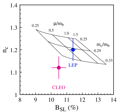
Figure 20: Theoretical Prediction (shaded region) of the semileptonic branching ratio and charm counting. The data points are the experimental results from high-energy (LEP) and low energy (i.e. at the $\Upsilon(4S)$ from CLEO) experiments.

This was the name given by Blok et al. [58] to the observation that the experimental value of the semileptonic branching ratio

$$B_{SL}=\frac{\Gamma(B\to Xe\bar{\nu})}{\sum_{l}\Gamma(B\to Xl\bar{\nu})+\Gamma_{had}+\Gamma_{rare}}$$ (154)

appeared to be lower than expected theoretically. In eq. (154) the sum is over the three species of lepton, and $\Gamma_{had}$ and $\Gamma_{rare}$ are the widths of the hadronic and rare decays respectively. Bigi et al. concluded that a branching ratio of less than 12.5% cannot be accommodated by theory [58]. Since then Bagan et al.  have completed the calculation of the $O(\alpha_{s})$ corrections, and in particular of the $b\to c\bar{c}s$ component of the decay (including the effects of the mass of the charm quark) [59]; these have the effect of decreasing $B_{SL}$. With M. Neubert, we used this input to reevaluate the branching ratio and charm counting ($n_{c}$, the average number of charmed particles per $B$-decay) [51] finding, e.g.

$$\begin{array}[]{ll}B_{SL}=12.0\pm 1.0\%\ (\mu=m_{b})&\ \ n_{c}=1.20\mp 0.06\ \ (\mu=m_{b})\\ B_{SL}=10.9\pm 1.0\%\ (\mu=m_{b}/2)&\ \ n_{c}=1.21\mp 0.06\ \ (\mu=m_{b}/2)\ .\end{array}$$ (155)

$\mu$ is the renormalization scale and the dependence on this scale is a reflection of our ignorance of higher order perturbative corrections. The experimental situation is somewhat confused, see Fig. 20. In his compilation at the ICHEP conference last year [60], Richman found that the semileptonic branching ratio obtained from $B$-mesons from the $\Upsilon(4S)$ is :

$$B_{SL}(B)=(10.23\pm 0.39)\%\ ,$$ (156)

whereas that from LEP is:

$$B_{SL}(b)=(10.95\pm 0.32)\%\ .$$ (157)

The label $b$ for the LEP measurement indicates that the decays from beauty hadrons other than the $B$-meson are included. Using the measured fractions of the different hadrons and their lifetimes, and assuming that the semileptonic widths of all the beauty hadrons are the same, one finds:

$$B_{SL}(b)=(10.95\pm 0.32)\%\Rightarrow B_{SL}(B)=(11.23\pm 0.34)\%\ ,$$ (158)

amplifying the discrepancy. It is very difficult to understand such a discrepancy theoretically, since the theoretical calculation only involves $\Gamma_{SL}$ (and not $\Gamma_{had}$ for which the uncertainties are much larger). In view of the experimental discrepancy, I consider the problem of the lifetime ratio $\tau(\Lambda_{b})/\tau(B^{0})$, described in subsection 4.2.1 above, to be the more significant theoretical one.

4.2.3 Exclusive Decays of $B$-Mesons

A large amount of experimental data is becoming available, particularly from the CLEO collaboration (see ref. [62] and references therein) on two-body (exclusive) nonleptonic decays of $B$-mesons. This is an exciting new field of investigation, which will undoubtedly teach us much about subtle aspects of the Standard Model. Unfortunately, at our present level of understanding we are not able to compute the amplitudes from first principles, and are forced to make assumptions about the non-perturbative QCD effects. Frequently these assumptions concern factorization, i.e. whether matrix elements of operators in the effective Hamiltonian which are products of two $V{-}A$ currents can be written in terms of products of matrix elements of the currents, e.g.

$$\langle D^{+}\pi^{-}|\,(\bar{d}u)_{L}\,(\bar{c}b)_{L}|\,B^{0}\rangle\stackrel{{\scriptstyle?}}{{=}}\langle D^{+}|\,(\bar{c}b)_{L}|\,B^{0}\rangle\ \langle\pi^{-}|\,(\bar{d}u)_{L}\,|\,0\rangle\ ,$$ (159)

where the first matrix element on the right hand side could be obtained from semileptonic decays (see sec. 2.1) and the second from the known value of $f_{\pi}$. In some cases, the factorization hypothesis can be motivated by the concept of colour transparency, that a light colour singlet meson, produced with large energy at the weak decay vertex (and which is hence a small colour-dipole), will travel a long way from the interaction region before it grows to a size where it could interact strongly [63, 64]. It is possible that in some cases factorization will give a reasonable first approximation and in many others it will not be useful at all. Thus current analyses are limited to a semi-quantitative level, and at this stage it is not possible to endorse any of the approaches. I will not discuss these analyses in these lectures, but to wish to point out the importance of this emerging field, (see refs. [65] and [40] for more extensive discussions).

5 Conclusions

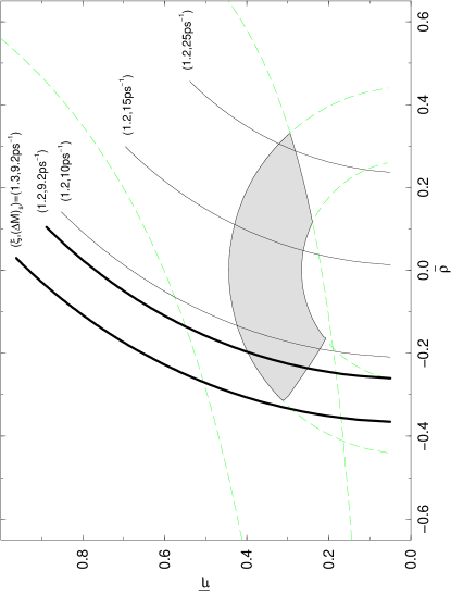
Figure 21: The current status of our knowledge of the position of the vertex $A$ of the unitarity triangle as obtained by Buras and Fleischer [1], (shaded area).

In these lectures I have briefly reviewed the formalism required for the study of the weak decays in the Standard Model of Particle Physics. From these studies we are attempting to measure the parameters of the Standard Model, to understand the origin of $CP$-violation and to look for signatures of physics beyond the Standard Model. I have explained that the major theoretical difficulty in interpreting the wealth of experimental data is our inability to control the non-perturbative strong interaction effects to sufficient precision. Througout these lectures I have illustrated the general discussion with applications to various physical processes. The current status of the uncertainties in determining the vertex $A$ of the unitarity triangle, from the analysis of Buras and Fleischer is reproduced in fig. 21. The circular arcs are obtained from information on $B-\bar{B}$ mixing, using a modified analysis to that discussed in section 3.2 above. In order to reduce the hadronic uncertainties, we can take the ratio of the expressions for $\Delta M_{B_{d}}$ and $\Delta M_{B_{s}}$ in eqs. (107) and (108), and, using the upper bounds on $\Delta M_{B_{d}}$ (0.482 ps^-1) and $|V_{ts}/V_{cb}|$ (0.993), obtain a bound for the quantity in eq. (113):

$$\frac{1}{\lambda}\frac{|V_{td}|}{|V_{cb}|}\,<\,1.0\,\xi\sqrt{\frac{10.2\,\textrm{ps}^{-1}}{\Delta M_{B_{s}}}}\ ,$$ (160)

where $\xi$ is defined in eq. (106), where the lattice result is also given. The curves in fig. 21 represent these bounds for several choices of $\xi$ and $\Delta M_{B_{s}}$ .

I end these lectures by summarising the tourist guide of Buras and Fleischer [1] to different processes, in which stars are awarded to the processes depending on the level of theoretical uncertainty.

1. These are processes in which there are no theoretical uncertainties i.e. they are particularly small (less than 2% say). Among these is the mixing-induced $CP$-violating asymmetry in $B_{d}\to J/\Psi K_{S}$ discussed in section 4.1.1, from which we expect to determine the angle $\beta$ of the unitarity triangle. Other quantities in this category which I have not had time to discuss include the ratio of (inclusive) branching ratios $\textrm{Br}(B\to X_{d}\nu\bar{\nu})/\textrm{Br}(B\to X_{s}\nu\bar{\nu})$ from which one would obtain $|V_{td}|/|V_{ts}|$ and the decays $K_{L}\to\pi^{0}\nu\bar{\nu}$ (which would give Im $\lambda_{t}$) and $K^{+}\to\pi^{+}\nu\bar{\nu}$ (which would give $|V_{td}|$). For the kaon decays I have explained in section 1.2.1, that the small mass difference between the quarks in the $K$ and $\pi$ mesons implies that the hadronic uncertainties are small.

2. The processes in this category have small hadronic uncertainties, of the order of 5-10% say. They include the evaluation of $V_{cb}$ discussed in sec. 2.1, $\Delta M_{d}/\Delta M_{s}$ discussed in section 3.2 (from which we obtain $|V_{td}|/|V_{ts}|$) and the mixing-induced $CP$-asymmetry in $B_{d}\to\pi^{+}\pi^{-}$ (from which we would obtain the angle $\alpha$) discussed in section 4.1.1. There is a large set of other mixing-induced asymetries in this category, yielding, in principle, all three angles. Being perhaps a little optimistic, the determination of $|V_{ub}|/|V_{cb}|$ in inclusive decays, also belongs to this category.

3. The processes in this category have smallish hadronic uncertainties, perhaps in the region of 15% or so. Of the quantities discussed in this course, $\Delta M_{d}$, $\Delta M_{s}$ (section 3.2) and $\epsilon$ (section 3.1.1) belong in this category.

4. As we have seen in these lectures, there are also important quantities for which the theoretical uncertainties are too large for the experimental data to give accurate information about the parameters of the Standard Model (and hence these quantities are not ascribed any stars), but which nevertheless give interesting qualitative information. These include $\epsilon^{\prime}/\epsilon$ (discussed in section 3.1.2) and most $CP$-asymmetries in decays of charged $B$’s. Non-leptonic decays of $B$-mesons in general belong to this category.

Of course it is to be hoped and expected that theoretical progress will continue, and that the interesting physical quantities will gradually acquire more stars. The theoretical community is working very hard to achieve this.

Acknowledgments

It is a pleasure to thank the students, lecturers and organisers of this school for providing such a lively and stimulating atmosphere. It was very thought-provoking and instructive to respond to the many excellent questions from the students without being able to rely on an armoury of theoretical formalism.

I warmly acknowledge my collaborators, particularly, Guido Martinelli and Matthias Neubert, with whom I learned many of the topics discussed in these lectures. I am grateful to Giulia de Divitiis and Luigi del Debbio for their comments on the manuscript.

References

- [1] A.J. Buras and R. Fleischer, hep-ph/9704376, to appear in Heavy Flavours (2nd edition), eds. A.J. Buras and M. Lindner, (World Scientific, Singapore, 1998)
- [2] J.F. Donoghue, E. Golowich and B.R. Holstein, Dynamics of the Standard Model (Cambridge University Press, Cambridge, UK, 1992)
- [3] -Decays 2nd edition, ed. S.Stone (World Scientific, Singapore, 1994)
- [4] -Violation, ed. C. Jarlskog, (World Scientific, Singapore, 1988)
- [5] J. Petersen, V. Zakharov, these proceedings
-
[6]
N. Cabibbo, Phys. Rev. Lett. 10 (1963) 531;
M. Kobayashi and T. Maskawa, Prog. Theo. Phys. 49 (1973) 652. - [7] R.M. Barnett et al., Phys. Rev. D54 (1996) 1
- [8] L. Wolfenstein, Phys. Rev. Lett. 51 (1983) 1945
- [9] E. Hagberg et al., nucl-ex/9609002
- [10] S.L. Glashow, J. Iliopoulos and L. Maiani, Phys. Rev. D2 (1970) 1285
- [11] P. Nason, these proceedings
- [12] M. Neubert, hep-ph/9702375, to appear in Heavy Flavours (2nd edition), eds. A.J. Buras and M. Lindner, (World Scientific, Singapore, 1998)
- [13] M. Luke, Phys. Lett. B252 (1990) 447
-
[14]
A. Czarnecki, Phys. Rev. Lett. 76 (1996)
4124;
A. Czarnecki and K. Melnikov Phys. Rev. Lett. 78 (1997) 3630 - [15] A. Falk and M. Neubert, Phys. Rev. D47 (1993) 2965 and 2982.
- [16] T. Mannel. Phys. Rev. D50 (1994) 428.
- [17] M.A. Shifman, N.G. Uraltsev and A.I. Vainshtein, Phys. Rev. D51 (1995) 2217.
- [18] I. Bigi, M. Shifman and N. Uraltsev, hep-ph/9703290
- [19] L. Di Ciaccio, to appear in the proceedings of the 7th International Symposium on Heavy Flavor Physics, Santa Barbara, California, July 1997
- [20] L.K. Gibbons, Proc. ICHEP96, 28th Int. Conf. on High Energy Physics, Warsaw, Poland, 25–31 July 1996, edited by Z. Ajduk and A.K. Wroblewski, World Scientific, Singapore (1997) p. 183
- [21] J.R. Patterson, Proc. ICHEP96, 28th Int. Conf. on High Energy Physics, Warsaw, Poland, 25–31 July 1996, edited by Z. Ajduk and A.K. Wroblewski, World Scientific, Singapore (1997) p. 871
- [22] N. Isgur and M. B. Wise, Phys. Rev. D42 (1990) 2388
- [23] P.A. Griffin, M. Masip and M. McGuigan, Phys. Rev. D42 (1994) 5751
- [24] H. Albrecht et al., Phys. Lett. B192 (1987) 245; Phys. Lett. B255 (1991) 297; R. Fulton et al., Phys. Rev. Lett. 64 (1990) 16; J. Bartelt et al., Phys. Rev. Lett. 71 (1993) 411
- [25] K. Symanzik, in Mathematical Problems in Theoretical Physics, eds. R. Schrader et al., Lecture Notes in Physics vol. 153 (Springer, New York, 1982); Nucl. Phys. B226 (1983) 187; Nucl. Phys. B226 (1983) 205
- [26] M. Lüscher and P. Weisz, Commun. Math. Phys. 97 (1985) 59; erratum Commun. Math. Phys. 98 (1985) 433
- [27] B. Sheikholeslami and R. Wohlert, Nucl. Phys. B259 (1985) 572
- [28] G. Heatlie et al., Nucl. Phys. B352 (1991) 266
- [29] M. Lüscher et al., Nucl. Phys. B478 (1996) 365; M. Lüscher and P. Weisz, Nucl. Phys. B479 (1996) 429; M. Lüscher et al., Nucl. Phys. B491 (1997) 323
- [30] G. Martinelli et al., Phys. Lett. B411 (1997) 141
- [31] K.G. Wilson, Phys. Rev. D10 (1974) 2445; K.G. Wilson, in New Phenomena in Subnuclear Physics, ed. A. Zichichi (Plenum Press, New York, 1975) p. 69
- [32] P. Lacock et al., Phys. Rev. D51 (1995) 6403
- [33] M. Bochicchio et al., Nucl. Phys. B262 (1985) 331; L.H. Karsten and J. Smit, Nucl. Phys. B183 (1981) 103; L. Maiani and G. Martinelli, Phys. Lett. B178 (1986) 265; G. Martinelli, S. Petrarca, C. T. Sachrajda and A. Vladikas, Phys. Lett. B311 (1993) 241; erratum Phys. Lett. B317 (1993) 660
- [34] G. Martinelli, C. Pittori, C.T. Sachrajda, M. Testa and A. Vladikas, Nucl. Phys. B445 (1995) 81
- [35] M. Lüscher, S. Sint, R. Sommer and H. Wittig, Nucl. Phys. B491 (1997) 344
- [36] SESAM and TL Collaborations, H. Hoeber et al., Proc. Lattice 97, 15th Int. Symp. on Lattice Field Theory, Edinburgh, Scotland, 1997, hep-lat/9709137
- [37] UKQCD Collaboration, J.M. Flynn et al., Nucl. Phys. B461 (1996) 327
- [38] A. Ali, V. Braun and H. Simma, Z. Phys C63 (1994) 437; P. Ball, Proc. 31st Rencontres de Moriond: Electroweak Interactions and Unified Theories, Les Arcs, France, March 1996, p. 365; V.M. Braun, Proc. Int. Europhysics Conf. on High Energy Physics, Brussels, Belgium, July 1995, p. 436; P. Ball and V.M. Braun, Phys. Rev. D55 (1997) 5561
- [39] J. Flynn and C.T. Sachrajda, hep-lat/9710057, to appear in Heavy Flavours (2nd edition), eds. A.J. Buras and M. Lindner, (World Scientific, Singapore, 1998)
- [40] C.T. Sachrajda, hep-ph/9711386, to be published in the proceedings of the 18th International Symposium on Lepton-Photon Interactions (LP97), Hamburg, Germany, 28 July - 1 Aug 1997
- [41] G.D. Barr et al., Phys. Lett. B317 (1993) 233
- [42] L.K. Gibbons et al., Phys. Rev. Lett. 70 (1993) 1203
- [43] J. Flynn, Proc. ICHEP96, 28th Int. Conf. on High Energy Physics, Warsaw, Poland, 25–31 July 1996, edited by Z. Ajduk and A.K. Wroblewski, World Scientific, Singapore (1997) p. 335
- [44] W.A. Bardeen, A.J. Buras and J.M. Gèrard, Phys. Lett. B211 (1988) 343; J.M. Gèrard, Acta Phys. Pol. B21 (1990) 257; J. Bijnens aand J. Prades, Nucl. Phys. B444 (1995) 523
- [45] A.J. Buras, M. Jamin and M.E. Lautenbacher, Phys. Lett. B389 (1996) 749
- [46] M. Ciuchini et al., Z. Phys C68 (1995) 239; M. Ciuchini, Nucl. Phys. B (Proc. Suppl.)59 (1997) 149
- [47] M. Gronau and D. Wyler, Phys. Lett. B265 (1991) 172
- [48] I.I. Bigi, B. Blok, M.A. Shifman, N.G. Uraltsev and A.I. Vainshtein, in -Decays (second edition), edited by S. Stone, (World Scientific, Singapore 1994), p. 132
- [49] I. Bigi, N. Uraltsev and A. Vainshtein, Phys. Lett. B293 (1992) 430; Erratum: Phys. Lett. B297 (1993) 477; B. Blok and M. Shifman, Nucl. Phys. B399 (1993) 441;Nucl. Phys. B399 (1993) 459;
- [50] Particle Data Group, R.M. Barnett et al., 1997 off-year partial update for the 1998 edition available on the PDG WWW pages (URL:http://pdg.lbl.gov/)
- [51] M. Neubert and C. T. Sachrajda, Nucl. Phys. B483 (1997) 339
- [52] M.A. Shifman and M.B. Voloshin, Sov. J. Nucl. Phys. 41 (1985) 120; JETP 64 (1986) 698; Sov. J. Nucl. Phys. 45 (1987) 292; H.D. Politzer and M.B. Wise, Phys. Lett. B206 (1988) 681; Phys. Lett. B208 (1988) 504
- [53] J. Rosner, Phys. Lett. B379 (1996) 267
- [54] M. Neubert, hep-ph/9707217, to appear in Proc. 2nd Int. Conf. on B Physics and CP Violation, Honolulu, Hawaii, March 1997
- [55] P. Colangelo and F. DeFazio, Phys. Lett. B387 (1996) 371
- [56] B. Blok, hep-ph/9707218; B. Blok, M. Shifman and D.X. Zhang, hep-ph/9709333
- [57] P. Colangelo, C. A. Dominquez and G. Nardulli, hep-ph/9705390
- [58] I.I. Bigi, B. Blok, M. Shifman and A. Vainshtein, Phys. Lett. B323 (1994) 408
- [59] E. Bagan, P. Ball, V. Braun and P. Gosdzinsky, Nucl. Phys. B432 (1994) 3, Phys. Lett. B342 (1995) 362 [Erratum Phys. Lett. B374 (1996) 363]; E. Bagan, P. Ball, B. Fiol and P. Gosdzinsky, Phys. Lett. B351 (1995) 546
- [60] J.D. Richman, Proc. ICHEP96, 28th Int. Conf. on High Energy Physics, Warsaw, Poland, 25–31 July 1996, edited by Z. Ajduk and A.K. Wroblewski, World Scientific, Singapore (1997) p. 143
- [61] M. Feindt, to appear in the Proceedings of the 1997 Europhysics Conference on High Energy Physics, Jerusalem, August 1997
- [62] P. Drell, hep-ex/9711011, to be published in the proceedings of the 18th International Symposium on Lepton-Photon Interactions (LP97), Hamburg, Germany, 28 July - 1 Aug 1997
- [63] J.D. Bjorken, in New Developments in High-Energy Physics, edited by E.G. Floratos and A. Vergazelakis, Nucl. Phys. B (Proc. Suppl.)11 (1989) 325
- [64] M.J. Dugan and B. Grinstein, Phys. Lett. B255 (1991) 583
- [65] M. Neubert and B. Stech, hep-ph/9705292; to appear in Heavy Flavours (2nd ed.), ed. by A.J. Buras and M. Linder (World Scientific, Singapore)