University of Wisconsin - Madison MADPH-97-1031 AMES-HET-97-13 December 1997

Abstract

We present a four-neutrino model with three active neutrinos and one sterile neutrino which naturally has maximal $\nu_{\mu}\rightarrow\nu_{\tau}$ oscillations of atmospheric neutrinos and can explain the solar neutrino and LSND results. The model predicts $\nu_{e}\rightarrow\nu_{\tau}$ and $\nu_{e}\rightarrow\nu_{\mu}$ oscillations in long–baseline experiments with $L/E\gg 1$ km/GeV with amplitudes that are determined by the LSND oscillation amplitude and argument controlled by the atmospheric $\delta m^{2}$.

There is growing experimental evidence that neutrinos oscillate [1]. The long-standing solar neutrino deficit [2, 3], the atmospheric neutrino anomaly [4, 5, 6], and the recent results from the LSND experiment on neutrinos from $\mu^{+}$ and $\pi^{+}$ decay [7] can all be understood in terms of oscillations between two neutrino species. The challenge is to describe all oscillation phenomena within a single model, since resonant oscillations for the sun, oscillations for the atmosphere, and the LSND data each require a different neutrino mass–squared difference $\delta m^{2}$ to properly describe all features of the data [8]. For example, if the atmospheric $\delta m^{2}$ scale is raised to the LSND scale, one forfeits the recently reported zenith–angle dependence of the atmospheric neutrino flux [5]. Alternatively, if the solar $\delta m^{2}$ is raised to the atmospheric $\delta m^{2}$ scale, one finds that: (i) the reduction in the solar neutrino flux is energy–independent [9], and (ii) near–maximal $\nu_{e}-\nu_{\mu}$ or $\nu_{e}-\nu_{\tau}$ mixing is necessary to describe the observed solar $\nu_{e}$ suppression; but in the context of a $3\times 3$ unitary matrix, such large mixing is inconsistent with the near maximal $\nu_{\mu}-\nu_{\tau}$ mixing deduced from the atmospheric data. Then also if $\delta m^{2}\geq 10^{-3}{\rm~{}eV}^{2}$, large $\nu_{e}$ mixing with any neutrino species is excluded by the recent CHOOZ reactor data [10]. Hence the large suppression of the solar flux can only result from resonance–enhancement, which requires a very small mass scale compared to those indicated by the atmospheric and LSND data. Since three-neutrino models can have at most two independent mass-squared differences $\delta m^{2}$, apparently not all the data can be explained with just $\nu_{e}$, $\nu_{\mu}$, and $\nu_{\tau}$.

A viable solution is to postulate one or more additional species of sterile light neutrino [11] without Standard Model gauge interactions (to be consistent with LEP measurements of $Z\rightarrow\nu\bar{\nu}$ [12]) thereby introducing another independent mass scale to the theory. The latter approach has been used with some success in the literature [13, 14]. The constraints of big-bang nucleosynthesis give the constraint

$$\delta m^{2}A<10^{-7}{\rm~{}eV}^{2}\;,$$ (1)

on the mass-squared difference $\delta m^{2}$ and oscillation amplitude $A=\sin^{2}2\theta$ for oscillations between a sterile neutrino and an active neutrino flavor [15].

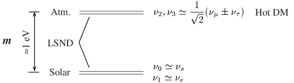
Figure 1: Neutrino mass spectrum, showing the approximate flavor content of each mass eigenstate, and showing which mass splittings are responsible for the LSND, atmospheric, and solar oscillations.

In this Letter, we examine a four-neutrino model (three active plus one sterile ) which naturally has maximal $\nu_{\mu}\rightarrow\nu_{\tau}$ oscillations of atmospheric neutrinos and which can also explain the solar neutrino and LSND results. We begin with a brief discussion of the three classes of experiments and the neutrino mass and mixing parameters needed to explain them. We then present a mass matrix whose eigenvalues consist of a nearly degenerate neutrino pair at $\sim 1$ eV and a nearly degenerate pair at low mass, as illustrated in Fig. 1. We show how the existing data almost uniquely fixes the model parameters and strictly determines what new phenomenology the model predicts. We find that the new observable signature for the model (in addition to the oscillations already indicated by the data) is $\nu_{e}\leftrightarrow\nu_{\mu}$ and $\nu_{e}\leftrightarrow\nu_{\tau}$ oscillations for $L/E\gg 1$ km/GeV. We discuss the possibility that such signals can be observed in long-baseline neutrino experiments such as those using intense muon sources at Fermilab [16] or KEK and detectors at SOUDAN, GRAN SASSO, or AMANDA as the target. We find that the SOUDAN and GRAN SASSO possibilities would probe some of the possible $\nu_{e}\rightarrow\nu_{\tau}$ oscillation region. We also compare this model to another four-neutrino mass matrix parameterization [14] which has been proposed to explain the data, and discuss their similarities and differences.

LSND. The LSND experiment [7] searches for $\bar{\nu}_{\mu}\rightarrow\bar{\nu}_{e}$ oscillations from $\mu^{+}$ decay at rest (DAR) and for $\nu_{\mu}\rightarrow\nu_{e}$ oscillations from $\pi^{+}$ decay in flight (DIF). The DAR data has higher statistics, but the allowed regions for the two processes are in good agreement and suggest $\nu_{\mu}\rightarrow\nu_{e}$ vacuum oscillation parameters that lie along the line segment described by

$$0.3{\rm~{}eV}^{2}\leq\delta m^{2}_{\rm LSND}={0.030{\rm~{}eV}^{2}\over(A_{\rm LSND})^{0.7}}\leq 2.0{\rm~{}eV}^{2}\;.$$ (2)

Larger values for $\delta m^{2}_{\rm LSND}$ are excluded at 90% C.L. by the BNL E-776 [17] and KARMEN [18] oscillation search experiments, and smaller values for $\delta m^{2}_{\rm LSND}$ are excluded by the Bugey reactor experiment, which looks for $\bar{\nu}_{e}$ disappearance [19]. If only 99% C.L. exclusion is required, $\delta m^{2}_{\rm LSND}$ as high as 10 eV² is allowed for $A_{\rm LSND}\simeq.0025$; values of $\delta m^{2}_{\rm LSND}>10$ eV² are excluded by the NOMAD experiment [20], while values above 3 eV² are disfavored by the r–process mechanism of heavy element nucleosynthesis in supernovae [21].

Atmospheric. The atmospheric neutrino experiments measure $\nu_{\mu}$ and $\nu_{e}$ (and their antineutrinos) created when cosmic rays interact with the Earth’s atmosphere. One expects about twice as many muon neutrinos as electron neutrinos from the resulting cascade of pion and other meson decays. Several experiments [4, 5] obtain a $\nu_{\mu}/\nu_{e}$ ratio that is about 0.6 of the value expected from detailed theoretical calculations of the flux [22]. The Super-Kamiokande experiment has collected the most data and a preliminary analysis indicates that their results can be explained as $\nu_{\mu}\rightarrow\nu_{\tau}$ oscillations with [1, 5, 6]

$$3\times 10^{-4}{\rm~{}eV}^{2}\leq\delta m^{2}_{\rm atm.}\leq 7\times 10^{-3}{\rm~{}eV}^{2}\,,\quad 0.8\leq A_{\rm atm.}\leq 1.0\;,$$ (3)

with the high end of each range favored. Although $\nu_{\mu}\rightarrow\nu_{s}$ oscillations (where $\nu_{s}$ is sterile) could in principle explain the atmospheric data, big-bang nucleosynthesis excludes this possibility [15] unless the chemical potential of the neutrinos is modified [23]. Independent of flux normalization considerations, the $\nu_{\mu}\rightarrow\nu_{e}$ oscillation channel is strongly disfavored by the zenith angle distributions of the data [5]. The recent CHOOZ $\bar{\nu}_{e}$ disappearance experiment also excludes $\bar{\nu}_{e}\rightarrow\bar{\nu}_{\mu}$ oscillations with large mixing $A\mathrel{\raisebox{-2.58334pt}{$\stackrel{{\scriptstyle\textstyle>}}{{\sim}}$}}0.2$ for $\delta m^{2}\geq 10^{-3}{\rm eV}^{2}$ [10].

Solar. The solar neutrino experiments [3] measure $\nu_{e}$ created in the sun. There are three types of experiments, $\nu_{e}$ capture in Cl in the Homestake mine, $\nu_{e}-e$ scattering at Kamiokande and Super-Kamiokande, and $\nu_{e}$ capture in Ga at SAGE and GALLEX; each is sensitive to different ranges of the solar neutrino spectrum and measures a suppression from the expectations of the standard solar model (SSM)[2]. Matter-enhanced MSW oscillations of $\nu_{e}\rightarrow\nu_{\mu},\nu_{\tau}$ [24], or $\nu_{s}$ [25] are sufficient to explain the data. For $\nu_{e}\rightarrow\nu_{s}$ the allowed parameter region [26] is bounded by

$$3.5\times 10^{-6}{\rm~{}eV}^{2}\leq\delta m^{2}_{\rm sol.}\leq 7.5\times 10^{-6}{\rm~{}eV}^{2}\,,\quad 2.5\times 10^{-3}\leq A_{\rm sol.}\leq 1.6\times 10^{-2}\;.$$ (4)

The allowed regions for small–angle MSW $\nu_{e}\rightarrow\nu_{\mu},\nu_{\tau}$ solutions are slightly smaller. However, if the LSND data is to be explained by $\nu_{\mu}\rightarrow\nu_{e}$ oscillations at the relatively large mass scale indicated in Eq. 2, and the atmospheric data by $\nu_{\mu}\rightarrow\nu_{\tau}$ oscillations with the much smaller scale of Eq. 3, then the solar neutrino data would appear to suggest $\nu_{e}\rightarrow\nu_{s}$ since the $\delta m^{2}_{e\tau}$ scale, which is also given by Eq. 2, is not consistent with Eq. 4. It is necessary that the eigenmass $m_{0}$ associated predominantly with $\nu_{s}$ be heavier than the mass $m_{1}$ associated predominantly with $\nu_{e}$ so that it is $\nu_{e}$ rather than ${\bar{\nu}}_{e}$ that is resonant in the sun, which requires

$$\delta m^{2}_{01}=m_{0}^{2}-m_{1}^{2}>0\;.$$ (5)

Complete description of the data. In order to explain all of the above data, one needs a model which includes the three different two-neutrino solutions described above. The appropriate mass scales $\delta m^{2}_{01}$ for MSW solar, $\delta m^{2}_{32}$ for atmospheric, and $\delta m^{2}_{21}\simeq\delta m^{2}_{31}\simeq\delta m^{2}_{31}\simeq\delta m^{2}_{31}$ for LSND oscillations are provided by the mass hierarchy $m_{1}^{2}\mathrel{\raisebox{-2.58334pt}{$\stackrel{{\scriptstyle\textstyle<}}{{\sim}}$}}m_{0}^{2}\ll m_{2}^{2}\simeq m_{3}^{2}$. Taking the small–angle solar MSW solution, the required oscillation amplitude hierarchy is $A_{es}\simeq A_{e\mu}\simeq A_{e\tau}\ll A_{\mu\tau}\simeq 1$.

Mass matrix ansatz. To describe the above oscillation phenomena, we consider the neutrino mass matrix

$$M=m\left(\begin{array}[]{cccc}\epsilon_{1}^{2}&\epsilon_{1}^{2}\epsilon_{2}&0&0\\ \epsilon_{1}^{2}\epsilon_{2}&0&0&\epsilon_{3}\\ 0&0&\epsilon_{4}^{2}&1\\ 0&\epsilon_{3}&1&\epsilon_{4}^{2}\end{array}\right)\;,$$ (6)

presented in the ($\nu_{s},\nu_{e},\nu_{\mu},\nu_{\tau}$) basis. The mass matrix $M$ contains five parameters ($m$, $\epsilon_{1}$, $\epsilon_{2}$, $\epsilon_{3}$, $\epsilon_{4}$), just enough to incorporate the required three mass differences and two small oscillation amplitudes $A_{e\mu}$ and $A_{es}$. The large amplitude $A_{\mu\tau}$ does not require a sixth parameter in our model, because the structure of the $\nu_{\mu}$–$\nu_{\tau}$ submatrix naturally gives maximal mixing here (more on this below). We note that changing the position of $\epsilon_{3}$ from the $M_{e\tau}$ element to the $M_{e\mu}$ element would cause the $\nu_{\tau}$ to oscillate into $\nu_{e}$ instead of into $\nu_{\mu}$. If nonzero terms are introduced at both the $M_{e\tau}$ and $M_{e\mu}$ positions, then the physics changes: both $\nu_{\mu}$ and $\nu_{\tau}$ would mix with $\nu_{e}$ at the LSND scale, and the $\nu_{e}-\nu_{s}$ mixing angle is also affected. Here we choose to take the minimal $M$ needed to describe the data and determine the consequences.

For simplicity, we have taken the mass matrix to be real and symmetric; then $M$ is diagonalized by an orthogonal matrix $U$. Since $U$ is real, there is no CP violation (which should be small anyway since observable CP–violation requires more than one large mixing angle, while the data seems to indicate just one). The $\epsilon_{j}$ are assumed to be small and of the same order of magnitude; phenomenologically they turn out to be within a factor of two of each other.

The smallness of $M_{es}/|M_{ss}-M_{ee}|=\epsilon_{2}$ is designed to yield the small-angle MSW solution for the sun. Simple changes in the 2x2 $\nu_{s}-\nu_{e}$ sub-block of $M$ would allow us to also consider the large–angle MSW solar solution, but since large mixing of sterile with active neutrinos is disfavored by the solar data [26] and big-bang nucleosynthesis [15] for these $\delta m^{2}$ values, we do not pursue this option here.

To a good approximation, the eigenvalues of the mass matrix in Eq. 6 are

$$m_{0}\simeq m\epsilon_{1}^{2}\,,\quad m_{1}\simeq m(\epsilon_{3}^{2}\epsilon_{4}^{2}-\epsilon_{1}^{2}\epsilon_{2}^{2})\,,\quad\textstyle m_{2,3}=\mp m\left(1\mp\epsilon_{4}^{2}+{1\over 2}\epsilon_{3}^{2}\right)\;,$$ (7)

which shows the desired hierarchy. The small relative mass splitting of the heavier masses $m_{2},m_{3}$ is governed entirely by the parameter $\epsilon_{4}^{2}$. Defining $\delta m^{2}_{ij}=m_{i}^{2}-m_{j}^{2}$, the LSND $\nu_{\mu}\rightarrow\nu_{e}$ oscillations are driven by the scale $m^{2}\simeq\delta m^{2}_{21}\simeq\delta m^{2}_{31}\simeq\delta m^{2}_{20}\simeq\delta m^{2}_{30}$, the atmospheric $\nu_{\mu}\rightarrow\nu_{\tau}$ oscillations are determined by $\delta m^{2}_{32}\simeq 4m^{2}\epsilon_{4}^{2}$, and the solar $\nu_{e}\rightarrow\nu_{s}$ oscillations are determined by $\delta m^{2}_{01}\simeq m^{2}\epsilon_{1}^{4}$. The charged-current eigenstates are approximately related to the mass eigenstates by

$$\left(\begin{array}[]{c}\nu_{s}\\ \nu_{e}\\ \nu_{\mu}\\ \nu_{\tau}\end{array}\right)=U\left(\begin{array}[]{c}\nu_{0}\\ \nu_{1}\\ \nu_{2}\\ \nu_{3}\end{array}\right)=\left(\begin{array}[]{cccc}1&-\epsilon_{2}&-{1\over\sqrt{2}}\epsilon_{1}^{2}\epsilon_{2}\epsilon_{3}&{1\over\sqrt{2}}\epsilon_{1}^{2}\epsilon_{2}\epsilon_{3}\\ \epsilon_{2}&1&{1\over\sqrt{2}}\epsilon_{3}&{1\over\sqrt{2}}\epsilon_{3}\\ -\epsilon_{2}\epsilon_{3}&-\epsilon_{3}&{1\over\sqrt{2}}&{1\over\sqrt{2}}\\ \epsilon_{2}\epsilon_{3}(\epsilon_{4}^{2}-\epsilon_{1}^{2})&\epsilon_{3}\epsilon_{4}^{2}&-{1\over\sqrt{2}}&{1\over\sqrt{2}}\end{array}\right)\left(\begin{array}[]{c}\nu_{0}\\ \nu_{1}\\ \nu_{2}\\ \nu_{3}\end{array}\right)\;.$$ (8)

Unitarity holds to first order in the $\epsilon_{j}$: $UU^{{\dagger}}=1+{\cal O}(\epsilon_{j}^{2})$. Note that $\nu_{0}$ and $\nu_{1}$ couple predominantly to $\nu_{s}$ and $\nu_{e}$, respectively, as desired. The near–degenerate $\nu_{2}$ and $\nu_{3}$ are seen to consist primarily of nearly equal mixtures of $\nu_{\mu}$ and $\nu_{\tau}$. These results are shown schematically in Fig. 1.

Oscillation probabilities. With real–valued $U$, the vacuum oscillation probabilities are, in general, given by [28]

$$P(\nu_{\alpha}\to\nu_{\beta})=\delta_{\alpha\beta}-4\sum_{i<j}U_{\alpha i}U_{\beta i}U_{\alpha j}U_{\beta j}\sin^{2}\Delta_{ji}\;,$$ (9)

where $\Delta_{ji}\equiv\delta m_{ji}^{2}L/4E=1.27(\delta m^{2}/{\rm eV}^{2})(L/{\rm km})/(E/{\rm GeV})$. For the mixing in Eq. 8, the off-diagonal vacuum oscillation probabilities, to leading order in $\epsilon_{j}$ for each $\Delta_{ij}$ and ignoring oscillations smaller than ${\cal O}(\epsilon_{j}^{4})$, are given by

$$P(\nu_{e}\to\nu_{\mu}) \simeq \epsilon_{3}^{2}\left(2\sin^{2}\Delta_{21}+2\sin^{2}\Delta_{31}-\sin^{2}\Delta_{32}\right)$$ (10)

$${}+\epsilon_{2}^{2}\epsilon_{3}^{2}\left(2\sin^{2}\Delta_{20}+2\sin^{2}\Delta_{30}-4\sin^{2}\Delta_{01}\right)\;,$$

$$P(\nu_{e}\to\nu_{\tau}) \simeq \epsilon_{3}^{2}\sin^{2}\Delta_{32}+2\epsilon_{3}^{2}\epsilon_{4}^{2}\left(\sin^{2}\Delta_{21}-\sin^{2}\Delta_{31}\right)\;,$$ (11)

$$P(\nu_{\mu}\to\nu_{\tau}) \simeq \sin^{2}\Delta_{32}+2\epsilon_{3}^{2}\epsilon_{4}^{2}\left(\sin^{2}\Delta_{31}-\sin^{2}\Delta_{21}\right)\;,$$ (12)

$$P(\nu_{e}\to\nu_{s}) \simeq 4\epsilon_{2}^{2}\sin^{2}\Delta_{01}\;,$$ (13)

$$P(\nu_{\mu}\to\nu_{s}) \simeq 4\epsilon_{2}^{2}\epsilon_{3}^{2}\sin^{2}\Delta_{01}\;,$$ (14)

where $\Delta_{01}\ll\Delta_{32}\ll\Delta_{20}\simeq\Delta_{30}\simeq\Delta_{21}\simeq\Delta_{31}$ due to the spectrum of the neutrino mass eigenvalues.

For small $L/E$ only the leading oscillations $\Delta_{20}\simeq\Delta_{21}\simeq\Delta_{30}\simeq\Delta_{31}$ contribute, and the only appreciable oscillation probability is

$$P(\nu_{e}\to\nu_{\mu})\simeq 4\epsilon_{3}^{2}\sin^{2}\Delta\;,$$ (15)

where $\Delta\equiv m^{2}L/4E$. From Eq. 15 we can fix two model parameters

$$\delta m^{2}_{\rm LSND}=m^{2}\;,\quad A_{\rm LSND}=4\epsilon_{3}^{2}\;.$$ (16)

The vacuum oscillation length associated with the LSND $\delta m^{2}$ scale is

$$\lambda_{v}=4\pi E/\delta m^{2}=2.5{\rm~{}km}(E/{\rm GeV})(\delta m^{2}_{\rm LSND}/{\rm eV}^{2})^{-1}\;.$$ (17)

For $L/E$ typical to atmospheric or long baseline neutrino experiments, the oscillations in $\Delta$ assume their average values. The $\Delta_{32}$ oscillation is now evident, and the non-negligible oscillation probabilities in vacuum are

$$P(\nu_{e}\to\nu_{\mu}) \simeq \epsilon_{3}^{2}\left(2-\sin^{2}\Delta_{32}\right)\;,$$ (18)

$$P(\nu_{e}\to\nu_{\tau}) \simeq \epsilon_{3}^{2}\sin^{2}\Delta_{32}\;,$$ (19)

$$P(\nu_{\mu}\to\nu_{\tau}) \simeq \sin^{2}\Delta_{32}\;.$$ (20)

From Eq. 20

$$\delta m^{2}_{\rm atm.}=\delta m^{2}_{32}\simeq 4m^{2}\epsilon_{4}^{2}\;,\quad A_{\rm atm.}=1\;,$$ (21)

which determines another parameter of the model. The model automatically gives maximal $\nu_{\mu}\rightarrow\nu_{\tau}$ oscillations for atmospheric neutrinos, while oscillations in other channels are suppressed. The $\nu_{\mu}$–$\nu_{\tau}$ maximal mixing is natural in the sense that it results from the large value of the $M_{\mu\tau}$ matrix element relative to the diagonal $M_{\mu\mu}$ and $M_{\tau\tau}$ elements, without any need for fine tuning of the difference $|M_{\mu\mu}-M_{\tau\tau}|$. The oscillation length resulting from the $\delta m^{2}_{32}$ scale is

$$\lambda_{v}=500{\rm~{}km}(E/{\rm GeV})(\delta m^{2}_{\rm atm}/5\times 10^{-3}{\rm eV}^{2})^{-1}\;.$$ (22)

Finally, for very large $L/E\gg(\delta m^{2}_{\rm atm.}/{\rm eV}^{2})^{-1}$ km/GeV, $\sin^{2}\Delta_{32}$ averages to ${1\over 2}$ and the appreciable oscillations in vacuum are (to leading order in the $\epsilon_{j}$)

$$P(\nu_{e}\to\nu_{s}) \simeq 4\epsilon_{2}^{2}\sin^{2}\Delta_{01}\;,$$ (23)

$$P(\nu_{e}\to\nu_{\mu}) \simeq {3\over 2}\epsilon_{3}^{2}\;,$$ (24)

$$P(\nu_{e}\to\nu_{\tau}) \simeq {1\over 2}\epsilon_{3}^{2}\;,$$ (25)

$$P(\nu_{\mu}\to\nu_{\tau}) \simeq {1\over 2}\;,$$ (26)

$$P(\nu_{\mu}\to\nu_{s}) \simeq 4\epsilon_{2}^{2}\epsilon_{3}^{2}\sin^{2}\Delta_{01}\;.$$ (27)

The solar data can then be explained with the usual MSW matter–enhanced mechanism (including the proper sign of $\delta m^{2}_{01}$ in Eq. 5) if the parameters in vacuum satisfy

$$\delta m^{2}_{\rm sol.}=\delta m^{2}_{01}\simeq 4m^{2}\epsilon_{1}^{4}\;,\quad A_{\rm sol.}=4\epsilon_{2}^{2}\;.$$ (28)

Summarizing the above analysis, the model parameters are related to the observables by

$$m^{2}=\delta m^{2}_{\rm LSND}\,,\quad\epsilon_{1}^{4}={\delta m^{2}_{\rm sol.}\over\delta m^{2}_{\rm LSND}}\,,\quad\epsilon_{2}^{2}={A_{\rm sol.}\over 4}\,,\quad\epsilon_{3}^{2}={A_{\rm LSND}\over 4}\,,\quad\epsilon_{4}^{2}={\delta m^{2}_{\rm atm.}\over 4\delta m^{2}_{\rm LSND}}\;.$$ (29)

For the specific values $\delta m^{2}_{\rm LSND}=2\rm~{}eV^{2}$, $A_{\rm LSND}=2.5\times 10^{-3}$, $\delta m^{2}_{\rm atm.}=5\times 10^{-3}\rm~{}eV^{2}$, $A_{\rm atm.}=1$, $\delta m^{2}_{\rm sol.}=4\times 10^{-6}\rm~{}eV^{2}$, and $A_{\rm sol.}=1\times 10^{-2}$, we obtain

$$m=1.4{\rm~{}eV}\,,\quad\epsilon_{1}=0.038\,,\quad\epsilon_{2}=0.050\,,\quad\epsilon_{3}=0.025\,,\quad\epsilon_{4}=0.025\,.$$ (30)

The corresponding neutrino mass eigenvalues are (in eV)

$$m_{0}=2\times 10^{-3}\,,\quad m_{1}=4\times 10^{-6}\,,\quad{1\over 2}(m_{3}+m_{2})\simeq 1.4\,,\quad{1\over 2}(m_{3}-m_{2})\simeq 9\times 10^{-4}\;.$$ (31)

For these masses $\sum m_{\nu}\approx 3$ eV, which according to recent work on early universe formation of the largest structures provides an ideal hot dark matter component [29].

If instead we use the lowest allowed mass scale for the LSND experiment we obtain $\delta m^{2}_{\rm LSND}=0.3\rm~{}eV^{2}$ and $A_{\rm LSND}=4\times 10^{-2}$, in which case

$$m=0.55{\rm~{}eV}\,,\quad\epsilon_{1}=0.060\,,\quad\epsilon_{2}=0.050\,,\quad\epsilon_{3}=0.10\,,\quad\epsilon_{4}=0.065\,,$$ (32)

with corresponding mass eigenvalues (in eV)

$$m_{0}=2\times 10^{-3}\,,\quad m_{1}=2\times 10^{-5}\,,\quad{1\over 2}(m_{3}+m_{2})\simeq 0.55\,,\quad{1\over 2}(m_{3}-m_{2})\simeq 2.3\times 10^{-3}\;.$$ (33)

In either of the above examples, the $\delta m^{2}$ scale for the atmospheric neutrino oscillation can be adjusted simply by varying $\epsilon_{4}$. Also in either case, the two heaviest masses provide relic neutrino targets for a mechanism that may generate the cosmic ray air showers observed above $\mathrel{\raisebox{-2.58334pt}{$\stackrel{{\scriptstyle\textstyle>}}{{\sim}}$}}10^{20}$ eV [30].

Model predictions. The model is constructed to provide the effective two-neutrino oscillation solutions for the LSND, atmospheric and solar data. The Solar Neutrino Observatory (SNO) [31], which can measure both charge-current (CC) and neutral-current (NC) interactions, will be able to test the $\nu_{e}\rightarrow\nu_{s}$ solar oscillation hypothesis: in the sterile case the CC/NC ratio in SNO would be unity and both CC and NC rates would be suppressed from the SSM predictions.

Given the order of magnitude of the $\delta m^{2}_{ij}$ and $U_{\alpha j}$, observable new phenomenology occurs for $L/E\gg 1$ km/GeV in the oscillation channels

$$P(\nu_{e}\rightarrow\nu_{\mu}) \simeq {1\over 4}A_{\rm LSND}(2-\sin^{2}\Delta_{\rm atm.})\;,$$ (34)

$$P(\nu_{e}\rightarrow\nu_{\tau}) \simeq {1\over 4}A_{\rm LSND}\sin^{2}\Delta_{\rm atm.}\;,$$ (35)

where $A_{\rm LSND}\sim{\cal O}(1\%)$ is the oscillation amplitude which describes the LSND results and $\Delta_{\rm atm.}=1.27\delta m^{2}_{\rm atm.}L/E\sim(\delta m^{2}_{\rm atm.}/5\times 10^{-3}{\rm~{}eV}^{2})(L/157{\rm km})({\rm GeV}/E)$ is the oscillation argument which describes the atmospheric neutrino data. In addition to the $\nu_{\mu}\rightarrow\nu_{e}$ oscillations due to $\Delta$ in Eq. 15, which reach their oscillation-averaged value of ${1\over 2}A_{\rm LSND}$, the model predicts new oscillations in the $\nu_{e}\rightarrow\nu_{\mu}$ and $\nu_{e}\rightarrow\nu_{\tau}$ channels with common oscillation length determined by $\Delta_{\rm atm.}$ and amplitude given by ${1\over 4}A_{\rm LSND}$.

How can the oscillation probabilities in Eqs.  34 and 35 be tested? A list of experiments currently underway or being planned to test neutrino oscillation hypotheses is given in Table 1 [32]. In each case the oscillation channel and the parameters which are expected to be tested are shown. Many of these experiments will not provide any constraints on the new phenomenology, although many provide some check on the existing LSND or atmospheric neutrino results (those that provide tests are noted in the table). The KARMEN upgrade, Booster Neutrino Experiment (BooNE at Fermilab), ORLANDO at Oak Ridge, and MINOS (Fermilab to SOUDAN) can test the LSND $\nu_{\mu}\rightarrow\nu_{e}$ oscillations, and for the experiments that probe $\delta m^{2}$ significantly below 1 eV², may be able to detect the contribution of the additional oscillation due to the $\sin^{2}\Delta_{32}$ term in Eq. 34. MINOS and ICARUS also aim to detect $\nu_{\tau}$ and should be able to probe some of the atmospheric neutrino allowed region for $\nu_{\mu}\rightarrow\nu_{\tau}$. NOMAD, CHORUS, and TOSCA at CERN and COSMOS at Fermilab will test $\nu_{\mu}\rightarrow\nu_{\tau}$ oscillations at most down to $\delta m^{2}\approx 0.1{\rm~{}eV}^{2}$ for maximum amplitude; these do not probe our model as there are no appreciable $\nu_{\mu}\rightarrow\nu_{\tau}$ oscillations in that region. Reactor experiments at Palo Verde in Arizona and with the BOREXINO detector in Europe will test $\bar{\nu}_{e}$ disappearance involving appreciable mixing angles, but will not test our model since the largest $\bar{\nu}_{e}$ vacuum oscillations are the $A=.04$ level or less.

Long-baseline experiments with an intense $\nu_{e}$ or $\bar{\nu}_{e}$ neutrino beam which can detect $\tau$’s, and hence see the $\nu_{e}\rightarrow\nu_{\tau}$ oscillations in Eq. 35, can provide a definitive test of the new phenomenology of our model. High intensity muon sources [16] can provide simultaneous high intensity $\nu_{\mu}$ and $\bar{\nu}_{e}$ (or $\bar{\nu}_{\mu}$ and $\nu_{e}$ for antimuons) beams with well-determined fluxes, which could then be aimed at a neutrino detector at a distant site. It is expected that $\tau$’s will be detected through their $\mu$ decay mode and that a charge determination can be made, so that one can tell if the $\tau$ originated from $\nu_{\mu}\rightarrow\nu_{\tau}$ or $\bar{\nu}_{e}\rightarrow\bar{\nu}_{\tau}$ oscillations. Current proposals [16] consider SOUDAN ($L=$ 732 km) or GRAN SASSO ($L=$ 9900 km) as the far site from an intense muon source at Fermilab. These experiments could also observe $\nu_{e}\rightarrow\nu_{\mu}$ oscillations via detection of “wrong-sign” muons. The neutrino energies are in the 10-50 GeV range. Assuming that low backgrounds can be achieved, the sensitivity to $\delta m^{2}$ is roughly proportional to the inverse square root of the detector size (given the same neutrino energy spectrum at the source); the $\delta m^{2}$ sensitivity does not depend on detector distance $L$ because although the flux in the detector falls off with $L^{2}$, the oscillation argument grows with $L^{2}$ for small $\delta m^{2}L/E$. For 20 GeV muons at Fermilab and a 10 kT detector at either SOUDAN or GRAN SASSO, the single-event $\delta m^{2}$ sensitivity for $\nu_{e}\rightarrow\nu_{\tau}$ oscillations is about $8\times 10^{-5}$ eV² for maximal mixing [16]. For large $\delta m^{2}$, the oscillation amplitude single-event sensitivity is roughly inversely proportional to the neutrino flux at the detector divided by the detector size; about $6\times 10^{-5}$ for SOUDAN and $10^{-2}$ for GRAN SASSO [16]. In general, the closer detector has comparable $\delta m^{2}$ sensitivity but better $A$ sensitivity.

Our model predicts $\nu_{e}\rightarrow\nu_{\tau}$ oscillations with amplitude $A_{\rm LSND}/4$ (which ranges from 0.0025 to 0.04) and mass-squared difference of $\delta m^{2}_{\rm atm.}$ (which ranges from $3\times 10^{-4}$ to $7\times 10^{-3}$ eV²). The region of possible $\nu_{e}\rightarrow\nu_{\tau}$ oscillations in our model and the regions which can be tested at the SOUDAN and GRAN SASSO sites are shown schematically in Fig. 2, along with the favored parameters for the LSND, atmospheric neutrino, and solar neutrino oscillations. Such experiments would be sensitive to some of the $\nu_{e}\rightarrow\nu_{\tau}$ region, though they may not cover the low-mass, small-amplitude part. These searches would also be able to test the $\nu_{e}\rightarrow\nu_{\mu}$ oscillations in Eq. 34 and the atmospheric $\nu_{\mu}\rightarrow\nu_{\tau}$ oscillations. Additionally, long baseline experiments to the AMANDA [33] detector from Fermilab or KEK may be useful in probing oscillations with small $\delta m^{2}$.

Neutrinoless double–$\beta$ decay. From the form of U and the mass eigenvalues one can readily see that neutrinoless double–$\beta$ decay is unobservable in our model. If neutrinos are Majorana particles, then the $(\beta\beta)_{0\nu}$ decay rate is proportional to

$$<m_{\nu}>\equiv|\sum_{j}U^{2}_{ej}m_{j}|\sim m\epsilon_{3}^{2}<10^{-2}{\rm eV}\;,$$ (36)

which is well below the present limit of $\sim$ 0.5 eV [27], and less than improved bounds realizable in the future. Note that possible CP–violating relative Majorana phases which we have ignored in our model can give smaller $<m_{\nu}>$ via a cancellation in the leading terms, but cannot give larger $<m_{\nu}>$.

Hot dark matter. The contribution of the neutrinos to the mass density of the universe is given by $\Omega_{\nu}=\sum m_{\nu}/(h^{2}93$ eV), where $h$ is the Hubble expansion parameter in units of 100 km/s/Mpc [34]; with $h=0.65$ our model implies $\Omega_{\nu}\approx 0.05$. An interesting test of neutrino masses is the Sloan Digital Sky Survey (SDSS) [35]. For two nearly degenerate massive neutrino species, sensitivity down to about 0.2 to 0.9 eV (depending on $\Omega$ and $h$) is expected, providing coverage of all or part of the LSND allowed range ($m=$0.55 to 1.4 eV in our model).

Resonant enhancement in matter. The curves in Fig. 2 assume vacuum oscillations. In general, large corrections to oscillations involving $\nu_{e}$ and $\nu_{s}$ are possible due to matter; the $\nu_{e}$ diagonal element in the effective mass-squared matrix receives an additional term $2\sqrt{2}G_{F}N_{e}E$ from the CC interaction, and the $\nu_{s}$ diagonal element receives the contribution $\sqrt{2}G_{F}N_{n}E$ (relative to the active neutrinos) because it does not have NC interactions, where $N_{e}$ and $N_{n}$ are the electron and neutron number density, respectively. In our model, however, these corrections do not significantly affect the large $m_{2}^{2}$ and $m_{3}^{2}$ mass eigenvalues as long as $E\ll$ 1 TeV, and hence only modify the $\delta m^{2}_{01}$ oscillation argument. For $E\geq 0.1$ GeV, the only significant change in the mixing parameters is that the $\nu_{e}-\nu_{s}$ mixing $\epsilon_{2}$ in Eqs. 10 to 14 is suppressed. The result is that for small and intermediate $L/E$ (i.e., all experiments described by Eqs. 15, 18, 19, and 20), matter does not appreciably change the observable phenomenology of the model. For large $L/E$, such as when $E\mathrel{\raisebox{-2.58334pt}{$\stackrel{{\scriptstyle\textstyle<}}{{\sim}}$}}10$ MeV for solar neutrinos, there can be maximal $\nu_{e}-\nu_{s}$ mixing which changes Eqs. 23, 24, and 27 to

$$P(\nu_{e}\to\nu_{s}) \simeq \sin^{2}\Delta_{01}\;,$$ (37)

$$P(\nu_{e}\to\nu_{\mu}) \simeq \epsilon_{3}^{2}\left({3\over 2}-\sin^{2}\Delta_{01}\right)\;,$$ (38)

$$P(\nu_{\mu}\to\nu_{s}) \simeq \epsilon_{3}^{2}\sin^{2}\Delta_{01}\;.$$ (39)

In this case the only significant effect of matter (other than the MSW enhancement of $\nu_{e}\rightarrow\nu_{s}$ that leads to the solar neutrino suppression) is to enhance the $\nu_{\mu}\rightarrow\nu_{s}$ oscillations and introduce a new oscillation in the $\nu_{e}\rightarrow\nu_{\mu}$ channel, although the amplitude of these new oscillations never gets above about 10^-2. Hence we conclude that the matter corrections for the mass matrix in Eq. 6 probably have no observable consequences.

Other models. Are other viable neutrino mixing schemes possible? A different form for the neutrino mass matrix is

$$M=m\left(\begin{array}[]{cccc}\epsilon_{1}^{2}&\epsilon_{1}^{2}\epsilon_{2}&0&0\\ \epsilon_{1}^{2}\epsilon_{2}&0&\epsilon_{3}&0\\ 0&\epsilon_{3}&1&\epsilon_{4}^{2}\\ 0&0&\epsilon_{4}^{2}&1+\epsilon_{5}^{2}\end{array}\right)\;.$$ (40)

This alternate form contains one more parameter, $\epsilon^{2}_{5}$, than the mass matrix in Eq. 6. Fine–tuning of this additional parameter is necessary to achieve maximal mixing in the $\nu_{2}-\nu_{3}$ sector. Eq. 40 is a generalization of the particular form used in Ref. [14] which has $\epsilon_{5}^{2}=2\epsilon_{4}^{2}$. Again, zero elements can be taken nonzero as long as they are very small. The eigenvalues are given approximately by

$$m_{0}\simeq m\epsilon_{1}^{2}\,,\quad m_{1}\simeq-m\epsilon_{3}^{2}\,,\quad m_{2,3}\simeq m\left[1+{1\over 2}(\epsilon_{3}^{2}+\epsilon_{5}^{2})\mp\sqrt{{1\over 4}(\epsilon_{3}^{2}-\epsilon_{5}^{2})^{2}+\epsilon_{4}^{4}}\right]\;.$$ (41)

The charged current eigenstates are approximately related to the mass eigenstates by

$$\left(\begin{array}[]{c}\nu_{s}\\ \nu_{e}\\ \nu_{\mu}\\ \nu_{\tau}\end{array}\right)=U\left(\begin{array}[]{c}\nu_{0}\\ \nu_{1}\\ \nu_{2}\\ \nu_{3}\end{array}\right)=\left(\begin{array}[]{cccc}1&-\beta\epsilon_{2}&\epsilon_{1}^{2}\epsilon_{2}\epsilon_{3}c&\epsilon_{1}^{2}\epsilon_{2}\epsilon_{3}s\\ \beta\epsilon_{2}&1&\epsilon_{3}c&\epsilon_{3}s\\ -\beta\epsilon_{2}\epsilon_{3}&-\epsilon_{3}&c&s\\ \beta\epsilon_{2}\epsilon_{3}\epsilon_{4}^{2}&\epsilon_{3}\epsilon_{4}^{2}&-s&c\end{array}\right)\left(\begin{array}[]{c}\nu_{0}\\ \nu_{1}\\ \nu_{2}\\ \nu_{3}\end{array}\right)\;.$$ (42)

where

$$\beta\equiv\epsilon_{1}^{2}/(\epsilon_{1}^{2}+\epsilon_{3}^{2})\;,$$ (43)

and

$$s\equiv\sin\theta_{\mu\tau}={1\over\sqrt{2}}\left[1+{{1\over 2}(\epsilon_{3}^{2}-\epsilon_{5}^{2})\over\sqrt{{1\over 4}(\epsilon_{3}^{2}-\epsilon_{5}^{2})^{2}+\epsilon_{4}^{4}}}\right]^{1/2}$$ (44)

determines the $\nu_{\mu}-\nu_{\tau}$ mixing and $c\equiv\cos\theta_{\mu\tau}$. We also have

$$\delta m^{2}_{sol.}=m^{2}_{0}-m^{2}_{1}\simeq m^{2}(\epsilon_{1}^{4}-\epsilon_{3}^{4})\,,\quad A_{sol.}\simeq 4\beta^{2}\epsilon_{2}^{2}\;.$$ (45)

Note that $m_{1}$ cannot be larger than $m_{0}$, since this would lead to a negative $\delta m^{2}_{\rm sol.}$ and would imply that $\bar{\nu}_{e}$ and not $\nu_{e}$ undergoes an MSW enhancement, contrary to the data. Hence $\epsilon_{1}$ must be larger than $\epsilon_{3}$ with this matrix form, which in turn limits $\beta$ to the interval $[0.5,1]$. Then $\epsilon_{2}$ must be raised by the factor $\beta^{-2}$ relative to the matrix form in Eq. 40 to give the proper MSW mixing. The LSND constraints are the same as in Eq. 16. In the $\nu_{\mu}-\nu_{\tau}$ sector, the parameters are determined by

$$\delta m^{2}_{\rm atm.}\simeq 2m^{2}\sqrt{(\epsilon_{3}^{2}-\epsilon_{5}^{2})^{2}+4\epsilon_{4}^{4}}\,,\quad A_{\rm atm.}\simeq{4\epsilon_{4}^{4}\over(\epsilon_{3}^{2}-\epsilon_{5}^{2})^{2}+4\epsilon_{4}^{4}}\;.$$ (46)

In this scenario the $\epsilon_{3}$ term significantly affects not only the lightest mass eigenvalue but also the mass splitting and mixing angle of the two heavy states. Consequently, some fine–tuning is necessary to achieve the proper phenomenology. Maximal mixing occurs only when $\epsilon_{3}\simeq\epsilon_{5}$, in which case $\delta m^{2}_{\rm atm.}=4m^{2}\epsilon_{4}^{2}$ just like our previous scenario. However, in the absence of such fine–tuning, submaximal mixing is probable, in which case a different value for $\epsilon_{4}$ is required to generate the correct $\delta m^{2}_{\rm atm.}$.

We may again solve for the parameters directly in terms of the observables. In the present case there are six parameters and six observables including the (now) possibly non–maximal amplitude for atmospheric oscillations. The result is

$$m^{2}=\delta m^{2}_{\rm LSND}\,,\quad\epsilon^{4}_{1}=\frac{\delta m^{2}_{\rm sol.}}{\delta m^{2}_{\rm LSND}}+\frac{A^{2}_{\rm LSND}}{16},$$ (47)

$$\epsilon_{2}^{2}=\frac{A_{\rm sol.}}{4}\left[1+\frac{A_{\rm LSND}\sqrt{\delta m^{2}_{\rm LSND}}}{\sqrt{A^{2}_{\rm LSND}\delta m^{2}_{\rm LSND}+16\delta m^{2}_{\rm sol.}}}\right]\,,\quad\epsilon_{3}^{2}=A_{\rm LSND}/4\,,$$ (48)

$$\epsilon_{4}^{2}=\frac{\sqrt{A_{\rm atm.}}\delta m^{2}_{\rm atm.}}{4\delta m^{2}_{\rm LSND}}\,,\quad\epsilon_{5}^{2}-\epsilon_{3}^{2}=\pm\frac{1}{2}\sqrt{1-A_{\rm atm.}}\,\frac{\delta m^{2}_{\rm atm.}}{\delta m^{2}_{\rm LSND}}\,.$$ (49)

Since the matrix form in Eq. 40 requires some fine–tuning to explain the data, some higher order terms must be retained in the expressions for the parameters.

Using the same input parameters as before, including maximal mixing in the atmospheric neutrino experiments (which implies $\epsilon_{5}=\epsilon_{3}$), we find for the largest $\delta m^{2}_{\rm LSND}$ solution

$$m=1.4{\rm~{}eV}\,,\quad\epsilon_{1}=0.039\,,\quad\epsilon_{2}=0.070\,,\quad\epsilon_{3}=\epsilon_{5}=0.025\,,\quad\epsilon_{4}=0.025\,,$$ (50)

with mass eigenvalues (in eV)

$$m_{0}=2.1\times 10^{-3}\,,\quad m_{1}=0.9\times 10^{-3}\,,\quad{1\over 2}(m_{3}+m_{2})\simeq 1.4\,,\quad{1\over 2}(m_{3}-m_{2})\simeq 9\times 10^{-4}\;.$$ (51)

For the smallest $\delta m^{2}_{\rm LSND}$ solution, we obtain

$$m=0.55{\rm~{}eV}\,,\quad\epsilon_{1}=0.103\,,\quad\epsilon_{2}=0.070\,,\quad\epsilon_{3}=\epsilon_{5}=0.100\,,\quad\epsilon_{4}=0.065\,,$$ (52)

with masses (in eV)

$$m_{0}=5.8\times 10^{-3}\,,\quad m_{1}=5.5\times 10^{-3}\,,\quad{1\over 2}(m_{3}+m_{2})\simeq 0.55\,,\quad{1\over 2}(m_{3}-m_{2})\simeq 2.3\times 10^{-3}\;.$$ (53)

In Eq. 52 some fine–tuning between $\epsilon_{5}$ and $\epsilon_{3}$ (to the 3% level) is needed for $\delta m^{2}_{\rm sol.}$ to have the correct sign and magnitude. In either Eq. 50 or 52 the mass scale for the atmospheric neutrino oscillation can also be adjusted simply by varying $\epsilon_{4}$ (for maximal mixing), or by adjusting $\epsilon_{4}$ and $\epsilon_{5}$ (for non-maximal mixing). The only new phenomenology is again $\nu_{e}\rightarrow\nu_{\mu},\nu_{\tau}$ for $L/E\gg 1$ km/GeV, except that $\sin^{2}\Delta_{\rm atm.}$ in Eqs. 34 and 35 is now replaced by $A_{\rm atm.}\sin^{2}\Delta_{\rm atm.}$ when $A_{\rm atm.}\neq 1$. The possible $\nu_{e}\rightarrow\nu_{\tau}$ oscillation amplitude is reduced by a factor $A_{\rm atm.}$ (which is apparently 0.8 or higher), which shifts the predicted region in Fig. 2 slightly to the left; otherwise this model is very similar to the model of Eq. 6.

Summary. In this letter we have presented a four-neutrino model with three active neutrinos and one sterile neutrino which naturally has maximal $\nu_{\mu}\rightarrow\nu_{\tau}$ oscillations of atmospheric neutrinos and can also explain the solar neutrino and LSND results. The model predicts $\nu_{e}\rightarrow\nu_{\tau}$ and $\nu_{e}\rightarrow\nu_{\mu}$ oscillations in long–baseline experiments with $L/E\gg 1$ km/GeV with amplitudes that are determined by the LSND oscillation amplitude and $\delta m^{2}$ scale determined by the oscillation scale of atmospheric neutrinos. Neutrino beams from an intense muon source at Fermilab or KEK with a detector at the SOUDAN or GRAN SASSO sites may be able to test part of the parameter region for these oscillations channels.

Acknowledgements. We thank K. Hagiwara and R.J.N. Phillips for discussions. This work was supported in part by the U.S. Department of Energy, Division of High Energy Physics, under Grants No. DE-FG02-94ER40817 and No. DE-FG02-95ER40896 and in part by the University of Wisconsin Research Committee with funds granted by the Wisconsin Alumni Research Foundation.

Table 1: Current and planned neutrino oscillation experiments. Check-marks denote accessible oscillation channels. The $\delta m^{2}$ and $\sin^{2}2\theta$ sensitivies are given.

									Test Model?
Experiment	$\displaystyle\nu_{\mu}\atop{\displaystyle\downarrow\atop\displaystyle\nu_{e}}$	$\displaystyle\nu_{\mu}\atop{\displaystyle\downarrow\atop\displaystyle\nu_{\tau}}$	$\displaystyle\nu_{e}\atop{\displaystyle\downarrow\atop\displaystyle\nu_{\tau}}$	$\displaystyle\nu_{e}\atop{\displaystyle\downarrow\atop\displaystyle\nu_{e}}$	$\displaystyle\delta m^{2}\atop\vskip 12.0pt plus 4.0pt minus 4.0pt\rm(eV^{2})$	$\sin^{2}2\theta$	$\displaystyle\rm Test\atop\displaystyle\rm LSND?$	$\displaystyle\rm Test\atop\displaystyle\rm Atmos?$	$\displaystyle\nu_{\mu}\atop{\displaystyle\downarrow\atop\displaystyle\nu_{e}}$	$\displaystyle\nu_{e}\atop{\displaystyle\downarrow\atop\displaystyle\nu_{\tau}}$
BOONE	$\surd$				$10^{-2}$	$6\times 10^{-4}$	$\surd$
BOREXINO				$\surd$	$10^{-6}$	0.4
CHORUS		$\surd$			0.3	$2\times 10^{-4}$
COSMOS		$\surd$			0.1	$10^{-5}$
ICARUS, NOE,	$\surd$	$\surd$			$3\times 10^{-3}$	$4\times 10^{-2}$		p
AQUA-RICH, OPERA
KARMEN	$\surd$				$4\times 10^{-2}$	$10^{-3}$	$\surd$
KamLAND	$\surd$				$2\times 10^{-3}$	0.2
K2K	$\surd$				$2\times 10^{-3}$	$5\times 10^{-2}$
Fermilab/Gran Sasso	$\surd$	$\surd$	$\surd$		$8\times 10^{-5}$	$10^{-2}$	p	$\surd$	p	p
Fermilab/Soudan	$\surd$	$\surd$	$\surd$		$8\times 10^{-5}$	$6\times 10^{-5}$	$\surd$	$\surd$	$\surd$	p
MINOS	$\surd$	$\surd$			$10^{-3}$	$10^{-2}$	p	p	p
NOMAD		$\surd$			0.5	$3\times 10^{-4}$
ORLANDO, ESS	$\surd$				$3\times 10^{-3}$	$10^{-4}$	$\surd$
Palo Verde				$\surd$	$10^{-3}$	0.2
TOSCA		$\surd$			0.1	$10^{-5}$

p = partially

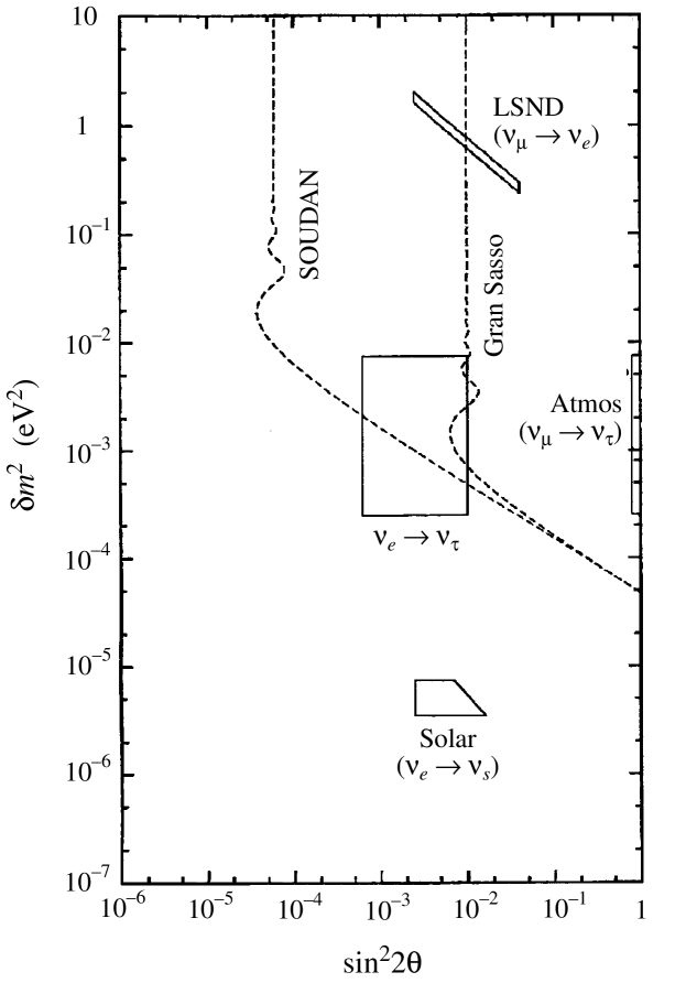
Figure 2: Predicted region in the effective $\delta m^{2}$-$\sin^{2}2\theta$ parameter space for $\nu_{e}\rightarrow\nu_{\tau}$ oscillations in the four-neutrino model (solid rectangle), which is determined by ${1\over 4}$ of the LSND $\nu_{\mu}\rightarrow\nu_{e}$ oscillation amplitude and the atmospheric neutrino $\nu_{\mu}\rightarrow\nu_{\tau}$ oscillation $\delta m^{2}$ scale. The dashed curves show the potential limits that can be set by neutrino beams from an intense muon source at Fermilab [16] to detectors at the SOUDAN and GRAN SASSO sites for muons with energy of 20 GeV. Also shown are the parameters for the solar $\nu_{e}\rightarrow\nu_{s}$ oscillation.

References

[1]
For a recent review, see talks at the ITP Conference on Solar Neutrinos:
News About SNUS, Santa Barbara, December 1997 at http://doug-pc.itp.ucsb.edu/online/snu/schedule.html
[3]
B.T. Cleveland et al., Nucl. Phys. B (Proc. Suppl.) 38, 47
(1995);
Kamiokande collaboration, Y. Fukuda et al., Phys. Rev. Lett,
77, 1683 (1996);
GALLEX Collaboration, W. Hampel et al., Phys. Lett. B388,
384 (1996);
SAGE collaboration, J.N. Abdurashitov et al., Phys. Rev. Lett.
77, 4708 (1996).
[4]
Kamiokande collaboration, K.S. Hirata et al., Phys. Lett.
B280, 146 (1992); Y. Fukuda et al., Phys. Lett.
B335, 237 (1994);
IMB collaboration, R. Becker-Szendy et al., Nucl. Phys. Proc.
Suppl. 38B, 331 (1995);
Soudan-2 collaboration, W.W.M. Allison et al., Phys. Lett. B391, 491 (1997).
[6]
J.G. Learned, S. Pakvasa, and T.J. Weiler, Phys. Lett. B207, 79 (1988);
V. Barger and K. Whisnant, Phys. Lett. B209, 365 (1988);
M.C. Gonzalez-Garcia, H. Nunokawa, O. Peres, T. Stanev, and J.W.F.
Valle, hep-ph/9712238.
[7]
Liquid Scintillator Neutrino Detector (LSND) collaboration,
C. Athanassopoulos et al., Phys. Rev. Lett. 75, 2650 (1995);
ibid. 77, 3082 (1996); nucl-ex/9706006.
[8]
G.L. Fogli, E. Lisi, D. Montanino, and G. Scioscia, Phys. Rev. D
56, 4365 (1997);
C.Y. Cardall and G.M. Fuller, Nucl. Phys. Proc. Suppl. 51B, 259 (1996);
A. Acker and S. Pakvasa, Phys. Lett. B397, 209 (1997);
Ernest Ma and Probir Roy, hep-ph/9706309.
[9]
P.I. Krastev and S.T. Petcov, Phys. Lett. B395, 69 (1997).
[10]
CHOOZ collaboration, M. Apollonio et al., hep-ex/9711002.
[11]
V. Barger, P. Langacker, J. Leveille, and S. Pakvasa, Phys. Rev. Lett.
45, 692 (1980);
J.R. Espinosa, hep-ph/9707541; G. Cleaver, M. Cvetic, J.R. Espinosa,
L. Everett, and P. Langacker, hep-ph/9705391.
[12]
LEP Electroweak Working Group and SLD Heavy Flavor Group,
D. Abbaneo et al., CERN-PPE-96-183, December 1996.
[13]
D.O. Caldwell and R.N. Mohapatra, Phys. Rev. D 48, 3259 (1993);
R. Foot and R.R. Volkas, Phys. Rev. D 52, 6595 (1995);
S.M. Bilenky, C. Giunti, and W. Grimus, hep-ph/9711416.
[14]
R.N. Mohapatra, hep-ph/9711444.
[15]
R. Barbieri and A. Dolgov, Phys. Lett. B237, 440 (1990);
K. Enqvist, K. Kainulainen, and M. Thomson, Nucl. Phys. B373, 498 (1992);
X. Shi, D.N. Schramm, and B.D. Fields, Phys. Rev. D 48, 2563 (1993);
C.Y. Cardall and G.M. Fuller, Phys. Rev. D 54, 1260 (1996);
D.P. Kirilova and M.V. Chizhov, hep-ph/9707282.
[16]
S. Geer, hep-ph/9712290.
[17]
L. Borodovsky et al., Phys. Rev. Lett. 68, 274 (1992).
[18]
KARMEN collaboration, B. Bodmann et al., Nucl. Phys. A553,
831c (1993); talk by K. Eitel at 32nd Rencontres de Moriond:
Electroweak Interactions and Unified Theories, Les Arcs, France,
March 1997, hep-ex/9706023.
[19]
Y. Declais et al., Nucl. Phys. B434, 503 (1995).
[20]
K. Zuber, talk at COSMO’97, Ambleside, England, September 1997, hep-ph/9712378.
[21]
Y.–Z. Qian et al., Phys. Rev. Lett. 71, 1965 (1993).
[22]
G. Barr, T.K. Gaisser, and T. Stanev, Phys. Rev. D 39,
3532 (1989);
M. Honda, T. Kajita, K. Kasahara, and S. Midorikawa, Phys. Rev.
D52, 4985 (1995);
V. Agrawal, T.K. Gaisser, P. Lipari, and T. Stanev, Phys. Rev.
D 53, 1314 (1996);
T.K. Gaisser et al., Phys. Rev. D 54, 5578 (1996).
[23]
R. Foot and R.R. Volkas, Phys. Rev. Lett. 75, 4350 (1995).
[24]
L. Wolfenstein, Phys. Rev. D 17, 2369 (1978);
S.P. Mikheyev and A. Smirnov, Yad. Fiz. 42, 1441 (1985);
Nuovo Cim. 9C, 17 (1986).
[25]
V. Barger, N. Deshpande, P.B. Pal, R.J.N. Phillips, and K. Whisnant,
Phys. Rev. D 43, 1759 (1991);
S. Bludman, D.C. Kennedy, and P. Langacker, Nucl. Phys. B374,
373 (1992).
[26]
N. Hata and P. Langacker, hep-ph/9705339.
[27]
H.V. Klapdor–Kleingrothaus, hep-ph/9712381.
[28]
V. Barger, K. Whisnant, D. Cline, and R.J.N. Phillips, Phys. Lett.
B93, 194 (1980).
[29]
For a recent discussion see J. Primack, astro-ph/9707285.
[30]
T.J. Weiler, hep-ph/9710431.
[31]
E. Norman et al., Solar Neutrino Observatory (SNO) collaboration,
in proc. of The Fermilab Conference: DPF 92, November 1992,
Batavia, IL, ed. by C. H. Albright, P.H. Kasper, R. Raja,
and J. Yoh (World Scientific, Singapore, 1993), p. 1450.
[32]
For World Wide Web links to more information on these and other
neutrino oscillation experiments, see the Neutrino Oscillation
Industry web page at
http://www.hep.anl.gov/NDK/Hypertext/nuindustry.html.
[33]
S. Barwick et al., AMANDA collaboration, in proc. XXVIth
International Conference on High Energy Physics, Dallas TX, August 1992,
ed. by James R. Sanford (AIP, New York, 1993), p. 1250; F. Halzen,
astro-ph/9707289.
[34]
E.W. Kolb and M.S. Turner, The Early Universe (Addison-Wesley,
Reading, 1990).
[35]
W. Hu, D.J. Eisenstein, and M. Tegmark, astro-ph/9712057.