Heavy Quark Hadroproduction in Perturbative QCD

Abstract

Existing calculations of heavy quark hadroproduction in perturbative QCD are either based on the approximate conventional zero-mass perturbative QCD theory or on next-to-leading order (NLO) fixed-flavor-number (FFN) scheme which is inadequate at high energies. We formulate this problem in the general mass variable-flavor-number scheme which incorporates initial/final state heavy quark parton distribution/fragmentation functions as well as exact mass dependence in the hard cross-section. This formalism has the built-in feature of reducing to the FFN scheme near threshold, and to the conventional zero-mass parton picture in the very high energy limit. Making use of existing calculations in NLO FFN scheme, we obtain more complete results on bottom production in the general scheme to order $\alpha_{s}^{3}$ both for current accelerator energies and for LHC. The scale dependence of the cross-section is reduced, and the magnitude is increased with respect to the NLO FFN results. It is shown that the bulk of the large NLO FFN contribution to the single heavy-quark inclusive cross-section is already contained in the (resummed) order $\alpha_{s}^{2}$ “heavy flavor excitation” term in the general scheme.

I Introduction

The production of heavy quarks in high energy processes has become an increasingly important subject of study both theoretically and experimentally [1]. The theory of heavy quark production in perturbative Quantum Chromodynamics (PQCD) is more challenging than that of light parton (jet) production because of the new physics issues brought about by the additional heavy quark mass scale. The correct theory must properly take into account the changing role of the heavy quark over the full kinematic range of the relevant process from the threshold region (where the quark behaves like a typical “heavy particle”) to the asymptotic region (where the same quark behaves effectively like a parton, similar to the well known light quarks $\left\{u,d,s\right\}$). Stimulated by significant recent experimental results on heavy quark production from HERA and the Tevatron, a number of theoretical methods have been advanced to improve existing QCD calculations of heavy quark production [2, 3, 4, 5], incorporating a dynamic role for the heavy quark parton. The purpose of this paper is to explain how the method of ACOT [2] is applied to heavy-quark production in hadron-hadron collisions, to compare results of this approach to existing “NLO” calculations, and to demonstrate that it satisfies some important consistency conditions.

Let us consider the production of a generic heavy quark, denoted by $H$, with non-zero mass $m_{H}$, in hadron-hadron collisions. We will define a quark as “heavy” if its mass is sufficiently larger than $\Lambda_{QCD}$ that perturbative QCD is applicable at the scale $m_{H}$, i.e., that $\alpha_{s}(m_{H})$ is small. Thus the $c$, $b$, and $t$ quarks are regarded as heavy, as usual. Let $Q$ be a typical large kinematic variable in the hard scattering process, in this case the $p_{T}$ of the heavy quark (or the associated heavy flavor hadron). The details of the physics of the heavy quark production process will then depend sensitively on the relative size of the two scales $m_{H}$ and $Q$. For simplicity, we will assume there is only one heavy quark – $H$ – that we need to treat. Extending our treatment to the real world case of $\left\{c,b,t\right\}$ quarks with successive higher masses is straightforward.

Conventional PQCD calculations involving heavy quarks consist of two contrasting approaches: the usual QCD parton formalism uses the zero-mass approximation ($m_{H}=0$) once the hard scale of the problem (say, $Q$) is greater than $m_{H},$ and treats $H$ just like the other light partons [6, 7, 8]; on the other hand, most recent “NLO” heavy quark production calculations consider $m_{H}$ as a large parameter irrespective of the energy scale of the physical process, and treat $H$ always as a heavy particle, never as a parton [9, 10, 11]. We shall refer to the former as the zero-mass variable-flavor-number (ZM-VFN) scheme – since the active flavor number varies, depending on the energy scale $\mu\sim Q$; and the latter as the fixed-flavor-number (FFN) scheme – since the parton flavor number is kept fixed, independent of $Q$.

Each of these approaches can only be accurate in a limited energy range appropriate for the approximation involved: $Q\gg m_{H}$ for the ZM-VFN scheme; and $Q\sim m_{H}$ for the FFN scheme. Nonetheless, both approaches have been used widely beyond their respective regions of natural applicability: on the one hand, NLO FFN calculations of $c$ and $b$ production are invoked from fixed-target to the highest collider energies [1]; and on the other hand, ZM-VFN calculations dominate practically all other standard model and new physics calculations, including most global PQCD analyses (which give rise to commonly used parton distributions [6, 7, 8]) and all popular Monte-Carlo event generators. The breakdown of the approximations beyond the original regions of applicability of these approaches can lead to unreliable results, and introduce large theoretical uncertainties. One possible sign of the latter is excessive dependence of theoretical predictions on the unphysical renormalization and factorization scale $\mu$ – which is well-known to be present in the NLO FFN calculation of hadro-production cross-section of $c$ and $b$ [12, 1].

With steadily improving experimental data on a variety of processes sensitive to the contribution of heavy quarks (including the direct measurement of heavy flavor production), it is imperative that the two diametrically opposite treatments of heavy quarks be reconciled in an unified framework which can also provide reliable theoretical predictions in the intermediate energy region, which in reality may well comprise most of the current experimentally relevant range for charm and bottom physics. This can be achieved in a general-mass variable-flavor-number (GM-VFN) scheme which retains the $m_{H}$ dependence at all energy scales, and which naturally reduces to the two conventional approaches in their respective region of validity [13, 14, 15, 2]. The method is a development of the one devised by Collins, Wilczek, and Zee [16]. The key point is that one can resum (and factor out) the mass singularities associated with the heavy quark mass $m_{H}$ into $H$ parton distribution and fragmentation functions without simultaneously taking the $m_{H}\rightarrow 0$ limit in the remaining infra-safe hard cross-section in the overall physical cross-section formula (as is routinely done in the ZM-VFN scheme). The resulting general formalism represents the natural extension of the familiar PQCD framework to include heavy quark partons both in the initial and final states of the hard scatterings which contribute to high energy processes in the SM and beyond.

The principles and the practical application of this method were described in some detail for (heavy quark parton contribution to) Higgs production in Ref. [14] and for lepto-production of heavy quarks in Ref. [15, 2]. It has been applied to the analysis of charm production in neutrino scattering [17], and, recently, to a new global QCD analysis of parton distributions [18]. In the present paper, we apply this general formalism to heavy quark production in hadron-hadron colliders. For a concise summary of this formalism, and related recent developments, see Ref. [3]; for a systematic proof of the factorization theorem which provides the theoretical foundation of this formalism, see Ref. [19]. In recent literature on leptoproduction of heavy quarks, there have been two other formulations of the VFN scheme with non-zero heavy quark mass: an order $\alpha_{s}$ scheme by Ref. [4] and an order $\alpha_{s}^{2}$ scheme by Ref. [5]. For definiteness, we shall refer to our implementation of the general principles as the ACOT scheme. Although not unique, it represents in many ways the simplest and the most natural one in relation to the familiar $\overline{\rm MS}$  ZM-VFN scheme [3]. See Ref. [20] for comments on some aspects of scheme dependence (in particular, mass-dependent or mass-independent evolution of the parton distributions), as well as on comparison to the scheme proposed by Ref. [4].

The following section presents details of our calculation scheme as applied to hadroproduction and describes the physical origin of the various terms which appear in the formalism. Sec. III contains specific information on how the various ingredients of the formalism are calculated. This is followed by numerical comparisons of the new calculation with existing FFN scheme results on the inclusive differential $p_{T}$ cross section for bottom production at current accelerator and LHC energies. In the concluding section, we discuss what remains to be done for a full understanding of heavy quark production in PQCD.

II Hadro-production of $H$ in the general mass formalism

Consider the hadro-production of a generic heavy quark $H$:

$$A+B\longrightarrow H+X$$ (1)

where $A$ and $B$ are hadrons, and $X$ includes $\overline{H}$ along with all other summed-over final state particles. In the ACOT formalism for heavy quark production developed in Refs. [13, 2, 19], the inclusive cross section for observing $H$ with a given momentum $p$ at high energies is given by a factorization formula of the same form as in the familiar zero-mass QCD parton formalism:

$$\sigma_{AB}^{HX}=\sum_{a,b,c}f_{AB}^{ab}\otimes\hat{\sigma}_{ab}^{c,r}\otimes d_{c}^{H},$$ (2)

where $\left\{A,B\right\}$ denote the initial state hadrons, $\left\{a,b\right\}$ the initial state partons, $f_{AB}^{ab}$ the associated parton distribution functions in the combination $f_{AB}^{ab}\equiv f_{A}^{a}f_{B}^{b}$, $\hat{\sigma}_{ab}^{c,r}$ the perturbatively calculable infra-red safe hard-scattering cross section for $\left\{a,b\right\}\rightarrow\left\{c,r\right\}$ which is free of large logarithms of $m_{H}$ over the full energy range, and $d_{c}^{H}$ the fragmentation functions for finding $H$ in $c$. All active partons are included in the summation over $\left\{a,b\right\}$ and $\left\{c\right\}$, including $H$ provided the renormalization and factorization scale $\mu$ is larger than $m_{H}$.

Since we shall compare our results to those of the FFN scheme, it is necessary to draw the distinction between the heavy quark $H$ and the associated light partons, we shall denote the latter collectively by $l$ for simplicity of notation. By definition, $l=\left\{g,q\right\}$ where $g$ is the gluon and $q$ denotes the light quarks in the sense of the FFN scheme: $q=\left\{u,d,s\right\}/\left\{u,d,s,c\right\}$ for charm/bottom production respectively. The number of light quark partons will be denoted by $n_{l}.$

As mentioned in the introduction, an important distinguishing feature of this general formalism from the familiar ZM-VFN parton approach is that, after subtraction of mass-singularities, the full $m_{H}$ dependence in the perturbatively calculated hard scattering coefficients $\hat{\sigma}_{ab}^{c,r}$ is retained. This allows the theory to maintain accuracy and reproduce the FFN scheme results in the threshold region, as required by physical considerations. On the other hand, our parton densities (and fragmentation functions) are defined in the $\overline{\rm MS}$  scheme, hence they satisfy mass-independent evolution equations — the same as in the usual zero-mass formalism. Considerable simplification then results in the implementation of this scheme since the well-established NLO evolution kernels and evolution programs can be directly used. It should be noted, however, that the parton densities do have implicit dependence on quark masses: to the leading power in $\Lambda/m_{H}$, this dependence is generated by the matching conditions at $\mu=m_{H}$ between the parton densities below and above the threshold — they are defined in each of the two regions by the respective renormalization scheme adopted for that region [13, 19].

The first few terms in the perturbative expansion of the production cross section, Eq. 2, are schematically

$$\begin{array}[]{rllrr}\sigma_{AB}^{HX}&=&f_{AB}^{ll^{\prime}}\,\otimes\,^{2}\hat{\sigma}_{ll^{\prime}}^{H\bar{H}}\otimes\,d_{H}^{H}&:&\text{HC0}\\ &&+f_{AB}^{lH}\,\otimes\,^{2}\hat{\sigma}_{lH}^{lH}\,\otimes d_{H}^{H}+f_{AB}^{Hl}\,\otimes\,^{2}\hat{\sigma}_{Hl}^{lH}\,\otimes d_{H}^{H}&:&\text{HE1}\\ &&+\,f_{AB}^{ll^{\prime}}\,\otimes\,^{3}\hat{\sigma}_{ll^{\prime}}^{H\bar{H}g}\otimes\,d_{H}^{H}&:&\text{HC1}\\ &&+f_{AB}^{ll^{\prime}}\,\otimes\,^{2}\hat{\sigma}_{ll^{\prime}}^{l_{1}l_{2}}\otimes d_{l_{1}}^{H}+f_{AB}^{Hl}\,\otimes\,^{2}\hat{\sigma}_{Hl}^{Hl}\otimes d_{l}^{H}&:&\text{GF1,2}\\ &&+f_{AB}^{HH}\,\otimes\,^{2}\hat{\sigma}_{HH}^{HH}\otimes d_{H}^{H}&:&\text{HH2}\end{array}$$ (3)

where repeated indices $l$, $l^{\prime}$, $l_{1}$, and $l_{2}$ are summed over all light flavors ($q$ and $g$) and the pre-superscript $n$ on ${}^{n}\hat{\sigma}$ denotes the formal order in the expansion of $\alpha_{s}$.

The physical interpretation of the various terms, labeled by the abbreviations in the last column of this equation, can be made apparent by the generic diagrams shown in Fig. 1. They are:

• HC0: the order $\alpha_{s}^{2}$ heavy flavor creation process $l~{}l^{\prime}\rightarrow H\,\bar{H}$ followed by heavy-quark fragmentation;

• HE1: the order $\alpha_{s}^{2}$ heavy flavor excitation process $l~{}H\rightarrow l~{}H$ followed by heavy-quark fragmentation;

• HC1: order $\alpha_{s}^{3}$ virtual and real corrections to HC0, $l~{}l^{\prime}\rightarrow H\bar{H}g,$ with fragmentation;

• GF1,2: order $\alpha_{s}^{2}$ (light- and heavy-) parton-gluon scattering $l~{}g\rightarrow l~{}\,g$ and $H~{}g\rightarrow H~{}g,$ followed by gluon fragmentation into the heavy quark $H$; and

• HH2: the order $\alpha_{s}^{2}$ $HH$ scattering $HH(\bar{H})\rightarrow HH(\bar{H}),$ with fragmentation.

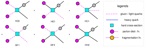
FIG. 1.: Graphical representation of the leading terms in the factorization formula which correspond to the various production mechanisms. The initial state hadron line for the parton distributions are uniformly suppressed.

For the diagrams in Fig. 1 we use a dashed line for all light partons $l$ (representing collectively gluons and light quarks) to distinguish them from the heavy quark $H$, represented by a solid line. The square blocks in these diagrams represent the hard cross sections ${}^{n}\hat{\sigma}$, obtained from all Feynman diagrams of the same order with the external lines indicated. The round blobs represent parton distribution and fragmentation functions. The initial state hadron lines for the parton distribution factors are suppressed in all the diagrams. For the differential cross section $d\sigma/dp_{T}^{H},$ the four terms involving $2\rightarrow 2$ hard scattering processes are tree-level processes. Beyond tree level, we have included only the most important order $\alpha_{s}^{3}$ term — HC1 — which contains $2\rightarrow 3$ real and $2\rightarrow 2$ virtual corrections to the leading HC0 cross-section. This term corresponds to the next-to-leading (NLO) contribution in the FFN scheme; it is known to be large and it is the only one that has been calculated to this order so far (see below). We will discuss the relative sizes of the various terms in the next paragraph, and comment on the possible significance of other terms not included here in later parts of the paper.

In conventional applications of PQCD with light partons, it is common to distinguish the order of terms in a cross section by treating the (non-perturbative) parton distributions in $f_{AB}^{ab}$ as all being of order one, and then counting powers of $\alpha_{s}$ in the hard scattering. With the inclusion of heavy quark partons, one may expect heavy quark distribution and fragmentation functions to be of order $\alpha_{s}$ in the energy region not too far above threshold, assuming they are purely radiatively generated. We know that at large $x$ the valence $u$ and $d$ quarks dominate all the other partons; while at small $x,$ it is the gluon density that dominates. For instance, in the latter region, we compare in Fig. 2 the relative sizes of the various sea partons at two energy scales to the gluon (scaled down by a factor of 5). In all cases it appears safe to regard the fully evolved heavy quark density $f_{A}^{H}$ to be of effective order $\alpha_{s}$ with respect to the dominant parton density (gluon or valence quark), i.e.,

$$f_{A}^{H}\sim{\cal O}(\alpha_{s})$$ (4)

Note, however, that the evolved charm density comes within a factor of 2 of the other sea quark densities at small $x$.

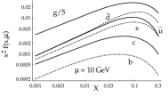
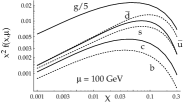
FIG. 2.: PDFs vs. $x$ for $\mu$ = 10 and 100 GeV. The gluon PDF is scaled by 1/5.

The same argument leads to the following expectations for the fragmentation functions (note, we confine ourselves to the production of the heavy flavor parton $H,$ rather than the associated hadron):

$$\begin{array}[]{lll}\,d_{H}^{H}&\sim&\delta(1-z)+{\cal O}(\alpha_{s})\\ d_{g}^{H}&\sim&{\cal O}(\alpha_{s})\\ d_{q,\bar{H}}^{H}&\sim&{\cal O}(\alpha_{s}^{2})\end{array}$$ (5)

These order-of-magnitude estimates are, of course, expected to become inapplicable at very large scales. The gluon-to-heavy-quark fragmentation function, in particular, can become substantial at large scales.

Nevertheless, let us use these estimates as the first guide to orders of magnitudes of the terms in Eq. 3. The first term (HC0) is of order $\alpha_{s}^{2}$; the HE1 and GF1 terms, and the HC1 term are of effective order $\alpha_{s}^{3}$; and the GF2 and the HH2 terms are of effective order $\alpha_{s}^{4}$. (This naive counting of effective order explains the choice of numerical suffixes in the labels for these terms.) The actual relative numerical importance of the various terms will also depend on other considerations such as large color factors or dynamical effects (e.g. spin-1 $t$-channel exchange contribution at high energies). This is well-known for the perturbative expansion of various processes, including heavy quark production calculated in the FFN scheme, where the order $\alpha_{s}^{3}$ NLO term (corresponding to HC1 without heavy quark mass subtractions) is actually larger than the order $\alpha_{s}^{2}$ LO term (HC0). We will examine in detail the numerical significance of the various terms in Sec. IV. The results are revealing, since they show simple features which are not accessible from the conventional FFN scheme perspective.

To specify fully the calculation in our scheme, we need to specify the perturbative hard cross sections $\hat{\sigma}_{ab}^{c,r}$. Following Ref. [2], we obtain these by applying the factorization formula, Eq. 2, to cross-sections involving partonic beams, that is to $\sigma_{ab}^{c,r}$ (without the caret) calculated from the relevant Feynman diagrams. Then we solve for the hard cross sections $\hat{\sigma}_{ab}^{c,r}$ order by order in $\alpha_{s}$. Specifically, in a given order $\alpha_{s}^{n},$ the factorization theorem implies that the partonic cross section has the form

$${}^{n}\sigma_{\alpha\beta}^{HX}=\sum\;^{n_{1}}f_{\alpha\beta}^{ab}\otimes\,^{n_{2}}\hat{\sigma}_{ab}^{c,r}\otimes\,^{n_{3}}d_{c}^{H},$$ (6)

where the sum is over the values of $n_{1}$, $n_{2}$, and $n_{3}$ that give the correct order, i.e., $n=n_{1}+n_{2}+n_{3}$. On the right-hand side, this equation differs from Eq. 2 in two respects. First, the parton distributions are relative to an on-shell parton target, instead of a hadron target. Secondly, we have expanded the parton-level distribution and fragmentation functions in powers of $\alpha_{s}$, with, for example, ${}^{n_{1}}f_{\alpha}^{a}$ denoting the term of $\alpha_{s}^{n_{1}}$ in the distribution function. These coefficients are calculated order by order in $\alpha_{s}$, but are not infra-red safe; they are used only in the intermediate steps toward the derivation of $\hat{\sigma}_{ab}^{c,r}$.

The most general method to obtain the hard scattering coefficients is directly from Eq. 6. All of the full partonic cross sections, the left-hand side, and the parton densities and fragmentation functions at the partonic level, on the right-hand side, can be computed from definite Feynman rules. From them, Eq. 6 gives the hard scattering coefficients. However, at the order $\alpha_{s}^{3}$ level to which we are working, it is convenient to carry out this calculation in two steps; the relation to the coefficient functions of the other schemes in the literature is then readily obtained.

First, the unsubtracted cross-sections are calculated from all relevant Feynman diagrams with the use of dimensional regularization (with the familiar parameters $\epsilon$ and $\mu$), with all light quark masses set to zero, and with the heavy quark mass non-zero. After ultra-violet renormalization (with $\overline{\rm MS}$ counter terms) and cancellation of infra-red divergences (after combining real and virtual diagrams), the cross-section formula will depend on the renormalized mass $m_{H}$ and the unphysical parameters ($\epsilon$ and $\mu$), in addition to the kinematic variables. The collinear singularities associated with the $1/\epsilon$ poles can be factorized into a kind of distribution function of light partons in a light parton $\bar{f}_{\alpha}^{a}(\epsilon,\mu)$ using the $\overline{\rm MS}$  convention. Since the cross-section is inclusive with respect to the light partons, we need no light parton fragmentation functions. Thus,

$${}^{n}\sigma_{\alpha\beta}^{HX}(m_{H},\epsilon,\mu)=\sum_{n_{1}+n_{2}=n}\;^{n_{1}}\bar{f}_{\alpha\beta}^{ab}(\epsilon,\mu)\otimes\,^{n_{2}}\tilde{\sigma}_{ab}^{HX}(m_{H},\mu),$$ (7)

where $\bar{f}_{\alpha\beta}^{ab}$ represents the product of two singular light parton distributions (cf. Eq. 2), and all non-essential (kinematical and convolution) variables have been suppressed. This concludes the first step of the construction, where the set of intermediate finite cross-sections ${}^{n}\tilde{\sigma}_{ab}^{HX}(m_{H},\mu)$ are obtained by systematically subtracting the collinear singularities.

At first sight, this appears to imply that the sub-set of ${}^{n}\tilde{\sigma}_{ab}^{HX}(m_{H},\mu)$ with $\left\{a,b\right\}=\left\{l,l^{\prime}\right\}$ (light partons) are the same as the conventional FFN scheme cross-sections. This is in fact true at the lowest non-trivial order, which is all that we will consider in this paper. However, at sufficiently high order extra heavy-quark loops come in, and these are renormalized differently in the FFN scheme and in the $\overline{{\rm MS}}$ scheme that we use when $\mu>m_{H}$. Hence the singularities to be subtracted differ by some kind of renormalization-group transformation. In this paper, we do not treat these higher order graphs.

The second stage of our calculation starts from the observation that although they are finite, the cross-sections ${}^{n}\tilde{\sigma}_{ab}^{HX}(m_{H},\mu)$ contain logarithmic mass-singularities, i.e. powers of $\ln\left(m_{H}/\mu\right)$, in the $m_{H}/\mu\rightarrow 0$ limit. The second step of the derivation consists of factoring these singularities out to arrive at the fully infra-red safe hard cross-sections ${}^{n}\hat{\sigma}_{ab}^{c,r}$ of Eq. 6. Explicitly,

$${}^{n}\tilde{\sigma}_{\alpha\beta}^{HX}(m_{H},\mu)=\sum\;^{n_{1}}\tilde{f}_{\alpha\beta}^{ab}\left(\ln(m_{H}/\mu)\right)\otimes\,^{n_{2}}\hat{\sigma}_{ab}^{c,r}(m_{H},\mu)\otimes\,^{n_{3}}\tilde{d}_{c}^{H}\left(\ln(m_{H}/\mu)\right).$$ (8)

Here the logarithmically singular terms in the $m_{H}\rightarrow 0$ limit are factored into $\tilde{f}$ and $\tilde{d}$. These are partonic level parton densities and fragmentation functions with subtractions made to remove the singularities associated with light partons. These subtractions exactly correspond to the subtractions used to obtain $\tilde{\sigma}$ from $\sigma$. The remaining infra-red safe $m_{H}$ dependence is kept in $\hat{\sigma}$ (in contrast to the conventional approach, where $m_{H}$ is set to zero).

As with all calculations of hard scattering coefficients, there is a freedom to choose exactly how to define the parton densities and fragmentation functions. The choice defines the factorization scheme, cf. [20], and thus determines how much of the finite $m_{H}$ dependence is included in $\tilde{f}$ and $\tilde{d}.$

We use the ACOT scheme [13, 2, 19]. In this scheme, the parton densities and fragmentation functions in the region $\mu>m_{H}$ are determined by the requirement that all ultra-violet divergences are renormalized by the $\overline{{\rm MS}}$ scheme — both the ultra-violet divergences in the renormalization of the interactions of QCD and the ultra-violet divergences that make finite the parton densities (in hadrons). The hard scattering coefficients $\hat{\sigma}$ in Eq. 6 are then well-defined. In the first stage of our calculation, the factorization of light parton singularities, we define the intermediate coefficients $\tilde{\sigma}$ in Eq. 7 by subtraction of collinear singularities in the $\overline{{\rm MS}}$ scheme.

Subtracting the terms which contain $\tilde{f}$ and $\tilde{d}$ with non-trivial mass singularities from ${}^{n}\tilde{\sigma}_{\alpha\beta}^{HX}(m_{H},\mu)$, we obtain the fully infra-red safe hard cross-sections ${}^{n}\hat{\sigma}_{ab}^{c,r}(m_{H},\mu)$ which we need in Eq. 2. The relevant non-vanishing perturbative parton distributions ${}^{n}\tilde{f}$ up to order $\alpha_{s},$ are:

$$\begin{array}[]{rll}{}^{0}\tilde{f}_{a}^{b}(x)&=&\delta_{a}^{b}\,\delta(1-x)\\ {}^{1}\tilde{f}_{a}^{H}(x,\mu)&=&\frac{\alpha_{s}(\mu)}{2\pi}\ \ln\left(\frac{\mu^{2}}{m_{H}^{2}}\right)\ P_{a\to H}(x)\\ {}^{1}\tilde{f}_{g}^{g}(x,\mu)&=&\frac{\alpha_{s}(\mu)}{2\pi}\ \ln\left(\frac{\mu^{2}}{m_{H}^{2}}\right)\ \delta(1-x)\end{array}$$ (9)

where $a,b=\{g,H\}$, $P_{a\to b}(x)$ is the usual first order splitting function. The only nonzero terms at order $\alpha_{s}$ in Eq. 9 come from contributions with a heavy quark loop. All one-loop corrections that involve light partons are zero, because of the well-known cancellation of IR and UV singularities. For the fragmentation functions, we have [22]:

$$\begin{array}[]{rll}{}^{0}\tilde{d}_{H}^{H}(z)&=&\delta(1-z)\\ {}^{1}\tilde{d}_{H}^{H}(z)&=&\frac{\alpha_{s}C_{F}}{2\pi}\left[\frac{1+x^{2}}{1-x}\left(\ln\frac{\mu^{2}}{M_{H}^{2}}-2\ln(1-x)-1\right)\right]_{+}\\ {}^{1}\tilde{d}_{g}^{H}(z,\mu)&=&\frac{\alpha_{s}(\mu)}{2\pi}\ \ln\left(\frac{\mu^{2}}{m_{H}^{2}}\right)\ P_{a\to b}(z)\end{array}$$ (10)

We can now substitute Eqs. 9 and 10 into Eq. 8 to solve for ${}^{n}\hat{\sigma}_{ab}^{c,r}.$ To order $\alpha_{s}^{2}$, only ${}^{0}\tilde{f}_{a}^{b}$ and ${}^{0}\tilde{d}_{a}^{b}$ are needed and we obtain the trivial identities,

$$\begin{array}[]{lll}{}^{2}\tilde{\sigma}_{l\,l^{\prime}}^{H\bar{H}}&=&{}^{2}\hat{\sigma}_{l\,l^{\prime}}^{H\bar{H}}\\ {}^{2}\tilde{\sigma}_{lH}^{lH}&=&{}^{2}\hat{\sigma}_{lH}^{lH}\\ {}^{2}\tilde{\sigma}_{HH}^{HH}&=&{}^{2}\hat{\sigma}_{HH}^{HH}\\ {}^{2}\tilde{\sigma}_{H\bar{H}}^{H\bar{H}}&=&{}^{2}\hat{\sigma}_{H\bar{H}}^{H\bar{H}}\end{array}$$ (11)

which reflect the fact that the order $\alpha_{s}^{2}$ cross sections are given by tree graphs: i.e. the ${}^{2}\tilde{\sigma}$’s are infra-red safe, in the $m_{H}\to 0$ limit. Hence they do not need any subtraction. Following the same procedure to order $\alpha_{s}^{3},$ we obtain schematically:

$${}{}\Sigma_{X}\,^{3}\tilde{\sigma}_{l\,l^{\prime}({\rm real+virtual})}^{H\bar{H}X} = {}\Sigma_{X}\,{}^{3}\hat{\sigma}_{l\,l^{\prime}}^{H\bar{H}X}$$ (14)

$$+\left[{}^{1}\tilde{f}_{g}^{g}\,\otimes\,{}^{2}\hat{\sigma}_{gl^{\prime}}^{H\bar{H}}+{}^{1}\tilde{f}_{g}^{g}\,\otimes\,{}^{2}\hat{\sigma}_{lg}^{H\bar{H}}\right]+{}^{2}\hat{\sigma}_{l\,l^{\prime}}^{H\bar{H}}\otimes\,^{1}\tilde{d}_{H}^{H}$$

$$+\left[{}^{1}\tilde{f}_{l^{\prime}}^{H}\otimes{}^{2}\hat{\sigma}_{lH}^{lH}+{}^{1}\tilde{f}_{l}^{H}\otimes{}^{2}\hat{\sigma}_{Hl^{\prime}}^{Hl^{\prime}}\right]+{}^{2}\hat{\sigma}_{ll^{\prime}}^{l_{1}l_{2}}\,\otimes\,^{1}\tilde{d}_{l_{1}}^{H}$$

For convenience, we have used a single equation to cover the various possible initial states. Not all terms on the right-hand side are applicable to all cases: for gluon-gluon scattering, $\left\{l\,l^{\prime}\right\}=\left\{gg\right\}$, all terms are present; for $\left\{l\,l^{\prime}\right\}=\left\{q\bar{q}\right\},$ only the 1st, 3rd and 5th terms contribute; and for $\left\{l\,l^{\prime}\right\}=\left\{gq(\bar{q})\right\},$ only the 1st, 4th and 5th terms contribute.

This equation can easily be inverted to obtain the order $\alpha_{s}^{3}$ hard cross section in terms of the calculated finite intermediate cross-sections ${}^{3}\tilde{\sigma}$ (with non-zero mass $m_{H})$ and various subtraction terms which remove the mass singularities associated with the heavy quark degree of freedom:

$$\begin{array}[]{lllrr}{}\Sigma_{X}\,^{3}\hat{\sigma}_{l\,l^{\prime}}^{H\bar{H}X}&=&{}\Sigma_{X}\,{}^{3}\tilde{\sigma}_{l\,l^{\prime}({\rm real+virtual})}^{H\bar{H}X}&\hskip 11.56346pt:&\mbox{HC1-FFN}\\ &&-{}^{1}\tilde{f}_{g}^{g}\otimes{}^{2}\tilde{\sigma}_{gg^{\prime}}^{H\bar{H}}-{}^{1}\tilde{f}_{g^{\prime}}^{g^{\prime}}\otimes{}^{2}\tilde{\sigma}_{gg^{\prime}}^{H\bar{H}}&:&\mbox{Fln-Sub}{}\\ &&-{}^{2}\tilde{\sigma}_{l\,l^{\prime}}^{H\bar{H}}\otimes\,^{1}\tilde{d}_{H}^{H}&:&\mbox{HF1-Sub}\\ &&-{}^{1}\tilde{f}_{l^{\prime}}^{H}\otimes{}^{2}\tilde{\sigma}_{lH}^{lH}-{}^{1}\tilde{f}_{l}^{H}\otimes{}^{2}\tilde{\sigma}_{Hl^{\prime}}^{Hl^{\prime}}&:&\mbox{HE1-Sub}\\ &&-{}^{2}\tilde{\sigma}_{ll^{\prime}}^{l_{1}l_{2}}\otimes{}^{1}\tilde{d}_{l_{1}}^{H}&:&\mbox{GF1-Sub}\end{array}$$ (15)

Here, we have replaced all tree-level ${}^{2}\hat{\sigma}$ in Eq. 11 by the corresponding ${}^{2}\tilde{\sigma}$ because they are the same, cf. Eq. 11. The content of the terms on the right-hand-side of this equation, labeled by the abbreviations in the last column, can be seen more easily from the diagrams in Fig. 3 where, for clarity, the four possible initial/final state channels are separately shown.

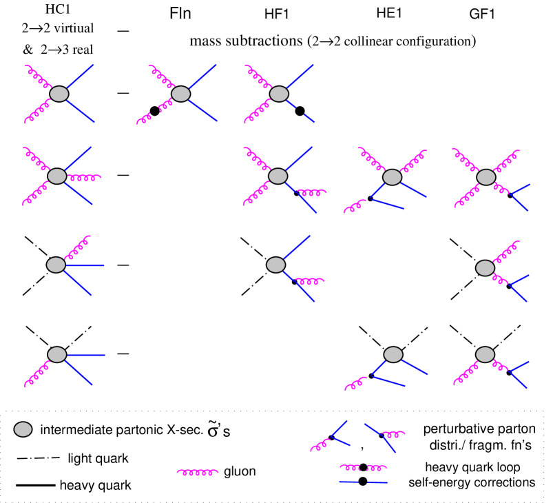
FIG. 3.: Graphical representation of the terms in the right-hand-side of Eq. 15. Collinear singularities due to light partons have already been subtracted. The vertices represented by a dot are the heavy quark parts of the perturbative distribution and fragmentation functions, as in Eqs. 9 and 10.

The terms in Eq. 15 and Fig. 3 are:

• HC1-FFN : the usual order $\alpha_{s}^{3}$ FFN scheme result, due to contributions of the NLO-HC (virtual and real) diagrams, with infra-red and collinear singularities associated with light partons cancelled/subtracted in the conventional way (in the $\overline{\rm MS}$  scheme);

• Fln-SUB : the correction to the order $\alpha_{s}^{2}$ gluon-gluon HC process due to the difference in the definition of the gluon distribution between the below-threshold ($n_{f}=n_{l}$) scheme and the above-threshold ($n_{f}=n_{l}+1$) scheme;

• HE-SUB : the subtraction of large logarithms of the heavy mass contained in ${}^{1}\tilde{f}_{g}^{H},$ cf.  Eq. 9, due to a flavor-excitation configuration;

• HF-SUB (GF-SUB) : the subtraction of large logarithms of the heavy mass in the final state heavy-quark (gluon) fragmentation residing in ${}^{1}\tilde{d}_{H,g}^{H},$ cf. Eq. 10.

After these subtractions, ${}^{3}\hat{\sigma}_{l\,l^{\prime}}^{H\bar{H}g}$ is free from all large logarithms associated with potential mass singularities, i.e. it is infra-red safe with respect to $m_{H}Q\rightarrow 0$. When this result is used in Eq. 3, the hadronic cross section is well-behaved in the high energy limit, in contrast to the FFN scheme result which would diverge because of the large logarithms. In fact, in this limit Eq. 3 reduces to the usual zero-mass $\overline{{\rm MS}}$ $\alpha_{s}^{3}$ parton formula with the $H$ quark counted just like the other light partons. This is, of course, the correct limit at high energies.

Some insight can be gained by explicitly substituting Eqs. 11, 15 in Eq. 3 and obtaining the hadronic cross section in terms of the intermediate partonic cross-sections $\left\{{}^{2}\tilde{\sigma},^{3}\tilde{\sigma}\right\}$ (which are all finite for non-zero $m_{H}$) along with the necessary subtraction terms which represent the overlap between the two sets of cross-sections and which remove the potentially dangerous mass singularities. The full set of terms are most clearly displayed in diagrammatic form, as shown in Fig. 4.

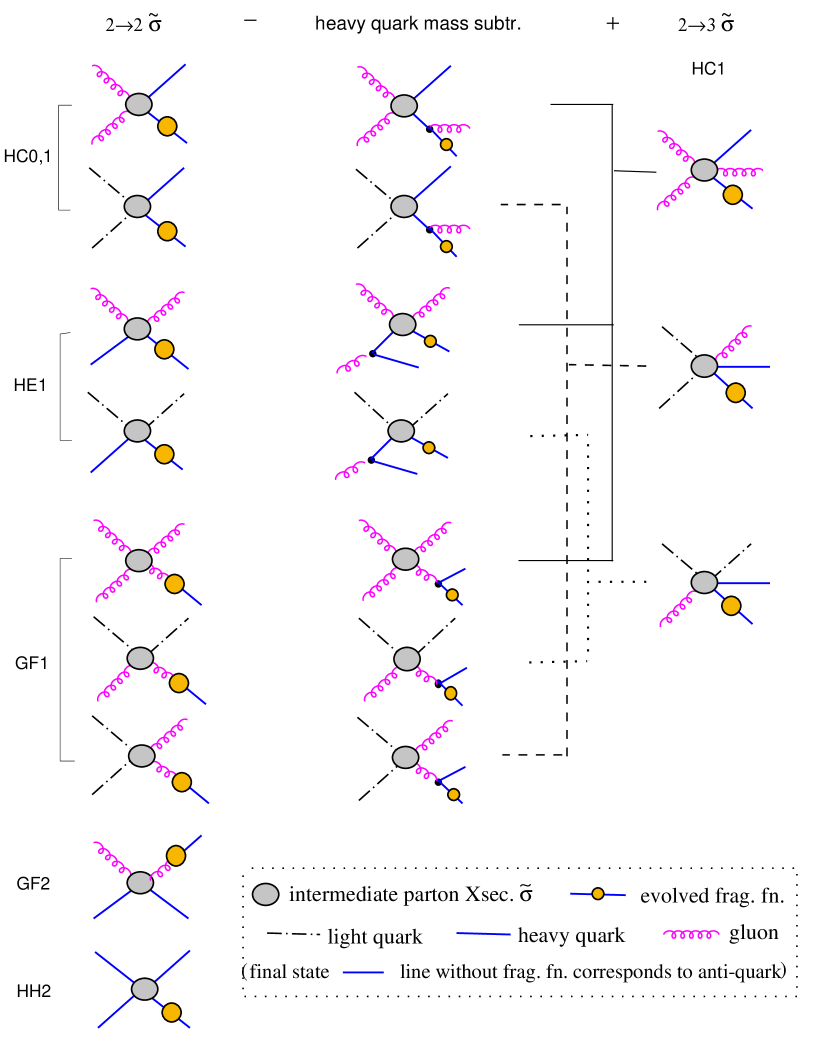
FIG. 4.: Graphical representation of the physical cross-section, Eq. 3 and Fig. 1, written in terms of the intermediate partonic cross-sections ${}^{n}\tilde{\sigma}$’s and the attendant heavy quark mass subtraction terms which represent the overlap between the 2$\rightarrow$2 and 2$\rightarrow$3 cross-sections. Initial state parton distribution function factors are uniformly suppressed.

The first column lists contributions from all the $2\rightarrow 2$ tree-level diagrams summarized in Eq. 3 and Fig. 1 plus 1-loop virtual corrections from Eq. 15; the last column lists contributions from all the $2\rightarrow 3$ terms contained in Eq. 15; and the middle column contains all the relevant subtraction terms. These terms can most easily be obtained by substituting the terms shown in Fig. 3 in those in Fig. 1, summing $l$ over $\left\{g,q\right\}$. With the exception of uniformly suppressing the initial state parton distribution factors (represented by dark blobs in Fig. 1), these diagrams contain all the ingredients needed to write down the full formula for the cross-section. In between the last two columns, we have also drawn lines to indicate the origins of the various subtraction terms in the $2\rightarrow 3$ diagrams, according to Fig. 3.

In this way of organizing the results, the order $\alpha_{s}$ subtraction terms in Fig. 4 are shown next to the relevant HE/GF/HF contributions in the same row, making explicit the physical origin of the subtractions: these terms containing large-logarithm (present in the un-regulated FFN scheme calculations) also represent the low-order components of the QCD evolved parton distribution/fragmentation functions. As an example, consider the first two terms in row one of HE1:

$${\rm(2}\rightarrow{\rm 2}\tilde{\sigma})-(m_{H}{\rm-subtraction}){\Big{|}}_{{\rm HE1}}^{gH\rightarrow gH}=f_{A}^{g}(f_{A}^{H}-f_{A}^{g}\,\otimes\,^{1}\tilde{f}_{g}^{H})\otimes\,^{2}\tilde{\sigma}_{gg}^{H\bar{H}}\otimes d_{H}^{H}$$ (16)

Both from this formula and from the corresponding graphs, one can see that the subtraction term containing $f_{A}^{g}\,\otimes\,^{1}\tilde{f}_{g}^{H}$ represents that part of the NLO-FFN contribution which is already included in the (fully evolved) parton distribution $f_{A}^{H}$. The latter, of course, represents the result of resumming all powers of $\alpha_{s}\ln\left(\mu^{2}/m_{H}^{2}\right)$, hence contains important physics not included in the NLO-FFN calculation, in addition to being well-behaved as $\mu^{2}/m_{H}^{2}$ becomes large — according to the renormalization group equation. Similar comments apply to the other 2$\rightarrow$2 $\tilde{\sigma}$ terms and the corresponding subtraction. The GF1 terms will be proportional to $(d_{g}^{H}-\,^{1}\tilde{d}_{g}^{H}\otimes d_{H}^{H})$ where $d_{g,H}^{H}$ are the fully evolved and $\,{}^{1}\tilde{d}_{g}^{H}$ the perturbative fragmentation functions.

The following (terms in) parton distribution and fragmentation functions $f_{A}^{H}$, ${}^{1}\tilde{f}_{g}^{H}$, ${}^{1}\tilde{f}_{g}^{g}$, and $d_{g}^{H}$ all vanish at the ‘threshold’, $\mu-m_{H}$ by calculation (cf. Eqs. 9,10 and Refs. [13, 2]). In addition, in the threshold region,

$$d_{H}^{H} \sim \delta(1-z)+O(\alpha_{s})$$ (17)

$$f_{A}^{H}-f_{A}^{g}\,\otimes\,^{1}\tilde{f}_{g}^{H} \sim O(\alpha_{s}^{2})$$ (18)

$$d_{g}^{H}-\,^{1}\tilde{d}_{g}^{H}\otimes d_{H}^{H} \sim O(\alpha_{s}^{2})$$ (19)

Hence, the differences between the first two columns of the terms represented in Fig. 4 — (2$\rightarrow$2 $\tilde{\sigma})-$heavy quark mass subtraction — vanish even faster than the individual terms approaching the threshold. Using these results, we obtain, in this limit

$$\begin{array}[]{rclrr}\sigma_{AB}^{HX}&\stackrel{{\scriptstyle\rm threshold}}{{\longrightarrow}}&\;\;f_{AB}^{l\,l^{\prime}}\,\otimes\,^{2}\tilde{\sigma}_{l\,l^{\prime}}^{H\bar{H}}&\hskip 11.56346pt:&\mbox{LO-FFN}\\ &&+\;f_{AB}^{l\,l^{\prime}}\,\otimes\,(\,^{3}\tilde{\sigma}_{l\,l^{\prime}\;{\rm(virtual)}}^{H\bar{H}}+\,^{3}\tilde{\sigma}_{l\,l^{\prime}\;{\rm(real)}}^{H\bar{H}l^{\prime\prime}})&:&\mbox{NLO-FFN}\\ &=&\;\;\tilde{\sigma}_{AB}^{HX}\;\;{\rm(full\;NLO-FFN\;scheme)}&&\end{array}$$ (20)

That is, the hadronic cross section in this formalism reduces to the full flavor creation (HC) result of the FFN scheme to order $\alpha_{s}^{3}$. In this region, there is effectively only one large momentum scale ($p_{T}\sim m_{H}$); and the FFN scheme is well suited to represent the correct physics.

We see, therefore, the ACOT formalism provides a natural generalization of the familiar light-parton pQCD to the case including quarks with non-zero mass which contains the right physics over the entire energy range. At high energies, Eq. 3 gives the most natural description of the underlying physics. The mass subtraction terms appearing in Eq. 15 for the $\alpha_{s}^{3}$ hard cross section correspond to the $\epsilon^{-1}$ poles arising from collinear singularities in the $m_{H}=0$ QCD parton formalism which are usually removed by $\overline{{\rm MS}}$ regularization. On the other hand, at energy scales comparable to the quark mass $m_{H}$, consistency with the physically sensible NLO-FFN calculation in the threshold region is also guaranteed by keeping the full $m_{H}$ dependence in the partonic cross sections appearing in Fig. 4, as described in the previous paragraph.

III Calculations

Our numerical calculations are carried out using Eq. 3, with hard cross sections given by Eqs. 11 and 15. (The equations are presented graphically in Fig. 4.) We briefly describe how the various quantities on the right-hand-side of the equation are obtained.

For the parton distributions $f_{A}^{a}(x,Q),$ we use the CTEQ3M set [8] for definiteness. The CTEQ parton distribution sets, in general, are evolved according to the ACOT scheme described in Ref. [2, 13, 16, 19] which is the one we use in the heavy quark production theory. This is necessary for obtaining consistent results (a point which has not been entirely obvious to all users of the scheme). The reason is: the expected compensation in the threshold region between the QCD-evolved $f_{A}^{H}(x,Q)$ and the perturbatively generated subtraction $f_{A}^{H}(x,Q)\,_{SUB}\equiv f_{A}^{g}(x,Q)\otimes\,^{1}\tilde{f}_{g}^{H}(x,Q)$ (cf. Eq. 16) will not take place unless the choice of evolution scheme and the choice of the location of the heavy quark threshold match properly. This is illustrated in Fig. 5 which compares $f_{A}^{H}(x,\mu)$ and $f_{A}^{H}(x,\mu)\,_{SUB}$ for charm and bottom as a function of $\mu$ at $x=0.1$ and $x=0.01$. Each curve individually vanishes at the threshold $\mu=m_{H}$ as required in this general scheme. As $\mu$ increases, both grow at a rapid rate because the evolution is driven by the large gluon distribution (through the mass-independent splitting kernel); however, the difference of the two, which determines the actual correction to the main contribution in this region (due to the HC process), grows slowly as one would expect on physical grounds. A failure to ensure the proper compensation between these terms due to a mismatch of schemes or the location of the threshold can lead to quite unphysical results because then the difference would be of the same order of magnitude as the individual terms.

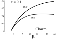
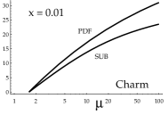
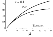
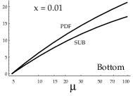
FIG. 5.: Comparison of the evolved PDFs, $f^{H}(x,\mu)$ (labeled PDF), and perturbative PDFs, ${}^{1}f^{H}(x,\mu)$ (labeled SUB), as a function of the renormalization scale $\mu$ for charm at $x=0.1$ (a) and $x=0.01$ (b), and for bottom at $x=0.1$ (c) and $x=0.01$ (d). This shows the compensation between fully evolved heavy quark parton distribution and the first order perturbative contribution (which is the only part contained in the FFN scheme calculation).

In calculating the partonic cross sections which appear in Eqs. 11 and 15, the formula for the LO-FFN cross sections ${}^{2}\tilde{\sigma}_{gg}^{HH}$ and ${}^{2}\tilde{\sigma}_{gH}^{gH}$ are well-known. For the NLO-FFN cross section, both virtual ${}^{3}\tilde{\sigma}_{gg}^{HH}$ and real ${}^{3}\tilde{\sigma}_{ll^{\prime}}^{HHl^{\prime\prime}}$, we used the Fortran codes from Ref. [11] and Ref. [23].

To calculate the gluon and heavy-quark fragmentation functions appearing in Eq. 3, we need also the QCD evolved fragmentation functions $d_{g,H}^{H}$. As mentioned earlier, for the purpose of this paper, we restrict ourselves to the $H$-quark production cross section; hence $d_{g,H}^{H}$ are parton to parton fragmentation functions. To obtain heavy flavor hadron production cross sections, it is necessary to perform an additional convolution with the appropriate hadronic fragmentation functions. The QCD evolved fragmentation functions $d_{g,H}^{H}(z,\mu)$ are generated by solving numerically the QCD evolution equation in our scheme, using as input at $\mu_{0}=m_{H}$ the perturbative formula, cf. Ref. [22, 24]. The comments about proper compensation between parton distributions made above also apply to the fragmentation functions $d_{g,H}^{H}$ and ${}^{1}\tilde{d}_{g,H}^{H}$. These features have been examined in detail during our calculation.

IV Results

We now present typical results for $b$ quark production cross section $\frac{d\sigma}{dp_{t}^{2}dy}|_{y=0}$ vs. $p_{t}$ and vs. the QCD scale parameter $\mu$ at collider energies. For simplicity, as is customary in the literature, we use a single scale parameter $\mu$ to represent the renormalization scale, the factorization scale for the parton distributions, and the factorization scale for the fragmentation functions. In principle, these could be chosen as independent; the hard cross sections would then depend on all three scales. As a rule, we shall express the scale $\mu$ as multiples of the natural physical scale $M_{T}\equiv\sqrt{p_{t}^{2}+m_{H}^{2}},$ although, again, other choices could also be considered. Except for explicit discussions concerning the $\mu$-dependence of the cross sections, our default choice of scale is $\mu^{2}=M_{T}^{2}/2$. In order to be able to clearly discern the various contributions to the steeply falling function $\frac{d\sigma}{dp_{t}^{2}dy}(p_{t})$, we shall in general use the scaled cross section $\ddot{\sigma}(p_{t})\equiv p_{t}^{5}\frac{d\sigma}{dp_{t}^{2}dy}|_{y=0}$ when examining its $p_{t}$ behavior. We concentrate mostly on b-production at the Tevatron for definiteness.

A Inclusive $p_{t}$ distribution and comparison of heavy parton picture in the FFN scheme

Fig. 6a shows $\ddot{\sigma}(p_{t})$ vs. $p_{t}$ for $b$ production at 1800 GeV, including the individual terms on the right-hand-side of Eq. 3. Over the range $10<p_{t}<100$ GeV, the two largest contributing terms are “leading order” ($2\rightarrow 2,$ tree-level) HE1 ($\hat{\sigma}_{gH\rightarrow gH}$) and HC0 ($\hat{\sigma}_{gg\rightarrow H\bar{H}}$); the other tree-level terms and the “next-to-leading” term, HC1 ($\hat{\sigma}_{gg\rightarrow gH\bar{H}},$ mass-subtracted), constitute about $10-25\%$ of the cross section, depending on the value of $p_{t}$. The left-hand-side plot shows the contributions from the individual terms; and the right-hand-side plot compares the relative sizes of the combined LO-VFN (i.e. tree-level) contribution, the NLO-VFN contribution and the total cross-section TOT-VFN when the calculation is organized in this scheme.

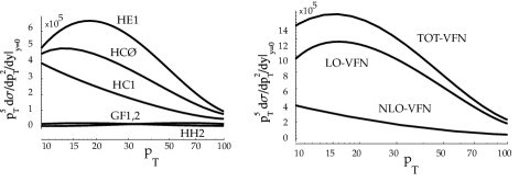
FIG. 6.: Contributions to the scaled cross section $p_{t}^{5}\,d\sigma/dp_{t}^{2}/dy|_{y=0}\ (nb\,{\rm GeV}^{3})$ vs. $p_{t}$ for $b$ production at 1800 GeV with $\mu=M_{T}/{\sqrt{2}}$ organized in the ACOT formalism. a) The curves correspond to the separate terms of Eq. 3. b) The curves are leading-order ($\alpha_{s}^{2}$) (LO-VFN), next-to-leading-order ($\alpha_{s}^{3}$) (NLO-VFN), and the total result (TOT-VFN).

Two interesting features are worth noting. First, the LO-VFN contributions (tree processes) give a reasonable approximation to the full cross section, the NLO-VFN correction is relatively small. (This is in sharp contrast to the situation in the familiar FFN scheme where the NLO-FFN term is bigger than the LO-FFN one. Cf. Fig. 7 and discussions below.) This is, of course, an encouraging result, suggesting that the heavy quark parton picture represents an efficient way to organize the perturbative QCD series. Secondly, the HE1 contribution is comparable to, and even somewhat larger than, the HCØ one – in spite of the smaller heavy quark parton distribution in the initial state compared to the gluon distribution. Closer examination reveals that two effects contribute to this non-apparent result: a larger color factor for the HE1 process, and the presence of $t$-channel gluon exchange diagrams which is absent in the HCØ process.

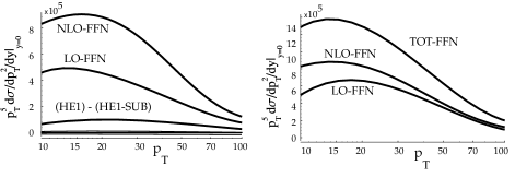
FIG. 7.: Contributions to the scaled cross section $p_{t}^{5}\,d\sigma/dp_{t}^{2}/dy|_{y=0}\ (nb\,{\rm GeV}^{3})$ vs. $p_{t}$ for $b$ production at 1800 GeV with $\mu=M_{T}/{\sqrt{2}}$ organized according to the FFN scheme. a) The curves correspond to the order $\alpha_{s}^{2}$ (LO-FFN) and order $\alpha_{s}^{3}$ (NLO-FFN) heavy-flavor creation (HC) contributions (without heavy mass subtractions). Also shown are the corrections due to the HE, GF1, GF2, and HH2 terms with associated subtractions as given in Fig. 4. The last three are numerically negligible and appear at the bottom of the plot unlabelled. Note that, (i) the NLO term is two times larger then the LO one; (ii) the contributions from are small and unlabeled. b) LO-FFN and NLO-FFN contributions along with the total result (TOT-FFN). Cf. Fig. 6 for comparison with the ACOT scheme case.

It is useful to compare the above situation with the same results organized in a way more familiar from the conventional FFN scheme point of view. For this purpose, one begins with the intermediate cross-sections $\tilde{\sigma}$ for heavy flavor creation processes only, HC0 ($\tilde{\sigma}_{gg\rightarrow H\bar{H}}$) and HC1 ($\tilde{\sigma}_{gg\rightarrow gH\bar{H}},$ no mass-subtraction). Corrections to the FFN scheme calculations in the full scheme then consist of the remaining terms on the right-hand-side of the cross section formula depicted in Fig. 4, which are now most naturally organized with the mass-subtraction terms combined with the corresponding $2\rightarrow 2$ cross-sections in the same row. Fig. 7a,b show $\ddot{\sigma}(p_{t})$ vs. $p_{t}$ in the same format as in the previous plot but with individual contributions organized in this way. The largest term is now the “NLO” HC1 ($\tilde{\sigma}_{gg\rightarrow gH\bar{H}}$) followed by the “LO” HC0 of the conventional FFN scheme. The fact that the NLO (order $\alpha_{s}^{3}$) term $\tilde{\sigma}_{HC1}$ is much larger than the LO term (order $\alpha_{s}^{2}$) $\tilde{\sigma}_{HC0}$ – the “K-factor” is typically of the order $\sim 2.5$ – is disturbing from the perturbation theory point of view, as has been known since the order $\alpha_{s}^{3}$ calculations were first done. On the other hand, we see from Fig. 7a, the corrections to the FFN scheme terms, consisting of the other terms in Fig. 4, are positive but not very large – again of the order of  $\stackrel{{\scriptstyle<}}{{\sim}}$ 20%. This means that the effects of resumming the collinear logarithms, represented by these additional terms, are modest for this case – a non-obvious result on account of the large K-factor and the significant $\mu$-dependence of the FFN scheme calculations (see next subsection). The net effect of these correction terms is to increase the theoretical cross-section. This is encouraging since the NLO FFN scheme result is known to be systematically smaller than the experimentally measured cross section at the Tevatron. However, this increase appears to fall short of the current observed discrepancy [1, 25]. Cf. Fig. 8.

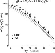
FIG. 8.: Comparison with experimental b-production data at the Tevatron $\sqrt{s}=1800$ GeV, $|y|<1$.[26, 27] The dashed lines represent the $\mu$-variation in the FFN scheme, and solid lines represent the $\mu$-variation in the VFN scheme. To gauge the $\mu$ scale variation, we choose $\mu=M_{T}/2$ for upper curves, and $\mu=2M_{T}$ for lower curves.

A comparison of Figs. 6 and 7 shows that, interestingly, the HE1 ($\hat{\sigma}_{HE1}$) contribution to the heavy quark production cross section in the heavy quark parton picture is quite comparable to the HC1 contribution in the complementary FFN scheme view ($\tilde{\sigma}_{HC1},$ no mass-subtraction) – to within about 10%. Thus, at least for this energy range, the heavy quark parton picture overlaps considerably with the FFN heavy flavor creation picture as far as the inclusive $p_{t}$ distribution is concerned — these two pictures are complementary rather than mutually exclusive, as sometimes perceived in the literature. It is, of course, much easier to calculate the tree-level HE1 cross section (a text book case) than the HC1 one (a tour de force). Thus, for this physical quantity, the heavy quark parton picture represents a much more efficient way to arrive at the right answer. This approximate equivalence between the HE1 and HC1 contributions to the inclusive $p_{t}$ cross section cannot, of course, be taken literally. The two contributions do not have the same ($s,\,p_{t},\mu,y$) dependence – in fact, the $\mu$ dependence can be rather different, as we will discuss next.

B Scale dependence of the cross section

In Fig. 9 we show a representative plot of $\sigma(p_{t},\mu)$ vs. $\mu$ at $p_{t}=20$ GeV. The tree-level HC0 and HE1 terms give the dominant contributions. In addition to the common $\alpha_{s}^{2}(\mu)$ factor, HC0 is predominantly driven by the gluon distribution, and this is a decreasing function of $\mu$. On the other hand, the tree-level HE1 term is driven by the heavy-quark distribution, and this is a increasing function of $\mu$. These two components compensate each other. Thus the full LO cross-section in the VFN ACOT scheme has a moderate $\mu$ dependence.

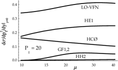
FIG. 9.: Scale ($\mu$) dependence of the leading ($\alpha_{s}^{2}$) order contributions to the cross section $d\sigma/dp_{t}^{2}/dy|_{y=0}\ (nb\,{\rm GeV}^{-2})$ for $b$ production at 1800 GeV with $p_{t}=20$ GeV in the ACOT formalism.

The situation is different for the FFN scheme, shown in Fig. 10. Here one finds that both the LO-FFN and NLO-FFN results (proportional to light parton distributions) are decreasing functions of $\mu$, resulting in a steep $\mu$ dependence for the combined result, TOT-FFN. If we were to compute higher order corrections in the FFN scheme, we would eventually observe compensating terms to reduce the $\mu$ dependence (as we know the “all-orders” result must be independent of $\mu$). The corrections to the FFN scheme result which have been resummed in the ACOT scheme into HE and GF contributions (minus subtractions) represent a part of these higher-order effect.

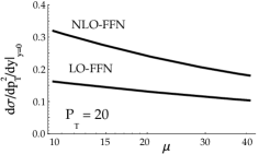
FIG. 10.: Scale ($\mu$) dependence of the main contributions to the cross section $d\sigma/dp_{t}^{2}/dy|_{y=0}\ (nb\,{\rm GeV}^{-2})$ for $b$ production at 1800 GeV with $p_{t}=20$ GeV organized in the FFN scheme.

In Fig. 11 we compare directly the TOT-FFN and the TOT-VFN results. The TOT-VFN result ranges from $\sim 5\%$ to $\sim 25\%$ above the TOT-FFN result depending on the choice of $\mu$. The additional resummed terms (labeled Difference) is seen to improve the $\mu$ dependence. (See also Fig. 13 below for LHC energies.)  Perhaps the improvement is not as complete as one might expect. This suggests there is still some non-negligible physics missing from the calculation. One possible source might be the NLO-HE process (HE2), on account of the large size of HE1. This is an ${\cal O}(\alpha_{s}^{3})$ contribution which has yet to be computed.

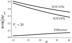
FIG. 11.: Comparison of the total cross section $d\sigma/dp_{t}^{2}/dy|_{y=0}\ (nb\,{\rm GeV}^{-2})$ in the ACOT and FFN formalism vs. $\mu$ for $b$ production at 1800 GeV with $p_{t}=20$ GeV. The Difference curve represents the additional resummed contributions included in the ACOT result.

Fig. 12 displays the scaled cross section vs. the physical variable  $p_{T}$ for the range of $\mu$ $[M_{T}/2,2M_{T}]$. The upper band corresponds to $\mu=M_{T}/2$, and the lower to $\mu=2M_{T}$. We see the increase in central value of the cross-section as well as the reduction in scale dependence in the ACOT scheme compared to the FFN scheme. The improvement is not dramatic in either case at this energy.

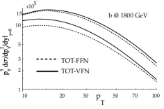
FIG. 12.: Variation of the total cross section $p_{t}^{5}\,d\sigma/dp_{t}^{2}/dy|_{y=0}\ (nb\,{\rm GeV}^{3})$ in the ACOT and FFN formalism vs. $p_{t}$ for $b$ production at 1800 GeV. To gauge the $\mu$ scale variation, we choose $\mu=M_{T}/2$ for upper curves, and $\mu=2M_{T}$ for lower curves.

One expects this to change at higher energies. Fig. 13 shows the corresponding results at the LHC energy of $\sqrt{s}=14\ TeV$. For comparison, we also present results for b-production at the CERN $Sp\bar{p}S$ energy of $\sqrt{s}=630\ GeV$ in Fig. 14.

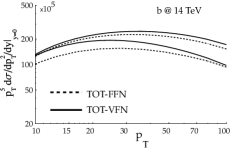
FIG. 13.: Same as Fig. 12, with $b$ production at 14 TeV.

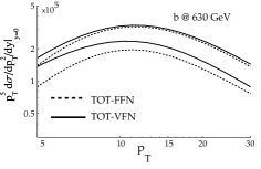
FIG. 14.: Same as Fig. 12, with $b$ production at 630 GeV.

C The Rapidity Distribution

Although the inclusive HE1 contribution in the ACOT was roughly comparable to the HC1 term in the FFN schemes, the dependence on the individual variables ($s,\,p_{t},\mu,y$) can be quite different. Having already investigated the $\mu$-dependence, we turn to the rapidity dependence of the underlying processes.

In Fig. 15 we compare the rapidity distribution for the HE1 and the HCØ  processes. To more easily compare the relative shape, we have scaled the two curves to equal area. We observe that the HE1 process yields a broader rapidity distribution than the HCØ  processes. In part, this is expected as the HE1 process includes a t-channel gluon exchange which can give an enhanced contribution in the forward direction. To see the relative effect on the rapidity distribution for the complete next-to-leading order calculations, in Fig. 16 we display the ratio of the TOT-VFN compared to the TOT-FFN cross section as a function of the rapidity.

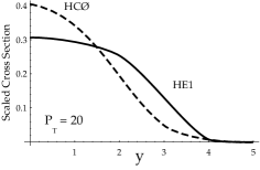
FIG. 15.: Comparison of the rapidity ($y$) distribution for the HCØ and HE1 processes for $b$ production at 1800 GeV with $p_{t}=20$ GeV and $\mu=M_{T}$. The curves are scaled to equal area to facilitate comparison of the shapes.

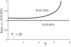
FIG. 16.: Comparison of the total cross section $d\sigma/dp_{t}^{2}/dy$ in the ACOT and FFN formalism vs. $y$ for $b$ production at 1800 GeV with $p_{t}=20$ GeV and $\mu=M_{T}$. The curves are scaled by the total FFN cross section to facilitate comparison of the relative magnitude.

D Comment on related work

It is worth mentioning that the resummation of large logarithms in the fixed-order calculations into parton distributions and fragmentation functions has also been studied by Cacciari and Greco [24]. In the notation of Eq. 2, their approach amounts to adopting the following ansatz for the hadro-production cross section:

$$\sigma_{AB}^{HX}=\sum_{a,b,c}f_{\left\{AB\right\}}^{\left\{ab\right\}}\otimes\hat{\sigma}_{ab}^{c,r}(m_{H}=0)\otimes d_{c}^{H}$$ (21)

where ($a,b,c$) are summed over all parton flavors including $H,$ and $\hat{\sigma}_{ab}^{c,r}(m_{H}=0)$ is given by the zero-mass (i.e. light-parton) NLO jet cross section calculation. This is a good approximation in the asymptotic region $p_{T}\gg m_{H},$ but it does not reproduce the right physics when $p_{T}$ is not significantly larger than the quark mass. The main result of their calculation was that the predicted $b$-production cross section has less scale dependence than the FFN scheme result, but it lies within the uncertainty band of the latter. Hence their predictions lie substantially below the experimental measurement and somewhat below our results. Our theory resums the same large logarithms associated with final state collinear singularities. But in addition, (i) we treat initial state parton distributions and final state fragmentations of the heavy quark symmetrically; and, more importantly, (ii) by keeping the heavy quark mass in the hard cross section according to the general factorization theorem, our results are applicable over the entire energy range. Strictly speaking, by using the order $\alpha_{s}^{3}$ jet cross section in Eq. 21, Ref. [24] includes higher order corrections to the corresponding terms in our calculation (GF1 and HF1 terms in Eq. 3). However, as shown above, the contribution from the latter is already small. Hence, the corrections are not expected to be important, and they are, in any case, of the same numerical order as NNLO flavor creation terms which are not currently calculated. Nonetheless, this difference may be responsible for the seemingly smaller $\mu$ dependence of their results. It is hard to be sure because their calculation is applicable only when $p_{T}\gg m_{H}$.

V Concluding Remarks

In this paper, we have systematically developed the theory for hadro-production of heavy quarks according to the natural pQCD scheme of Ref. [13, 15, 2, 19] which generalizes the conventional (zero-mass) “improved QCD parton model” to include quark mass effects. This formalism has the advantage that it contains the correct physics over a wide range of energies and $Q$ ($p_{T}$), and it reduces to the conventional results both at the low and the high energy limits. In particular, it coincides with the widely used FFN scheme in its natural region of applicability where $Q$ is or the same order of magnitude as $m_{H}$ – the one-large-scale region. Improvement over the FFN scheme results become important when $Q\gg m_{H}$. This is manifested both in the reduced theoretical uncertainty and in the increased cross-section. The improvement comes at the price of somewhat more complicated calculations. As seen in Eq.15 and Fig.4, in addition to the FFN scheme contributions, one needs to compute the other terms involving flavor excitation and fragmentation processes and their subtractions. As emphasized in Sec. III, these calculations must be done with care, due to the delicate cancellations required.

This more complete and consistent theory is, however, not a cure-for-all. Within our scheme, the residue scale dependence seen in Sec.IV may suggest that certain non-negligible higher order terms still need to be included. Our cross-section predictions, although higher than the existing FFN ones, still fall somewhat short of the $b$ cross-section measured at the Tevatron. Some physics effects not included in our formalism could be important: notably, those related to large logarithms of the type $\ln(Q^{2}/s),\ln(m_{H}^{2}/s)$ $\sim\ln x$ which needs to be separately resummed. This is another example of the small-x problem.[28] In this paper, we also have not addressed questions concerning the hadronization of the heavy quark which is not yet fully understood.

As an important physical process involving the interplay of several large scales, heavy quark production poses a significant challenge for further development of QCD theory.

REFERENCES

- [1] S. Frixione, M. L. Mangano, P. Nason, and G. Ridolfi, in Heavy Flavours II, edited by A. J. Buras and M. Lindner (unpublished), hep-ph/9702287; M. L. Mangano, hep-ph/9711337.
- [2] M. A. G. Aivazis, J. C. Collins, F. I. Olness, and W.-K. Tung, Phys. Rev. D 50, 3102 (1994).
- [3] W.-K. Tung, in Deep Inelastic Scattering and QCD, 5th International Workshop (DIS 97), edited by J. Repond and D. Krakauer (American Institute of Physics, Chicago, 1997), p. 1014.
- [4] A. D. Martin, R. G. Roberts, M. G. Ryskin, and W. J. Stirling, hep-ph/9612449.
- [5] M. Buza, Y. Matiounine, J. Smith, and W. L. van Neerven, hep-ph/9707263; hep-ph/9612398; M. Buza and W. L. van Neerven, Nucl. Phys. B500, 301 (1997).
- [6] E. Eichten, I. Hinchliffe, K. Lane, and C. Quigg, Rev. Mod. Phys. 56, 579 (1984); 58, 1065 (1986).
- [7] A. D. Martin, W. J. Stirling, and R. G. Roberts, Int. J. Mod. Phys. A10, 2885 (1995); Phys. Rev. D 50, 6734 (1994); Phys. Lett. B306, 145 (1993); B309, 492(E) (1993).
- [8] H. L. Lai et al., Phys. Rev. D 55, 1280 (1997); H. L. Lai et al., ibid. 51, 4763 (1995); J. Botts et al., Phys. Lett. B304, 159 (1993).
- [9] J. Collins, D. Soper, and G. Sterman, Nucl. Phys. B250, 199 (1985).
- [10] P. Nason, S. Dawson, and R. K. Ellis, Nucl. Phys. B303, 607 (1988); B327, 49 (1989); B335, 260(E) (1990).
- [11] W. Beenakker, H. Kuijf, W. L. van Neerven, and J. Smith, Phys. Rev. D 40, 54 (1989); W. Beenakker, W. L. van Neerven, R. Meng, G. A. Schuler, and J. Smith, Nucl. Phys. B351, 507 (1991).
- [12] G. Altarelli et al., Nucl. Phys. B308, 724 (1988).
- [13] J. C. Collins and W.-K. Tung, Nucl. Phys. B278, 934 (1986).
- [14] F. I. Olness and W.-K. Tung, Nucl. Phys. B308, 813 (1988).
- [15] M. A. G. Aivazis, F. I. Olness, and W.-K. Tung, Phys. Rev. D 50, 3085 (1994).
- [16] J. Collins, F. Wilczek, and A. Zee, Phys. Rev. D 18, 242 (1978).
- [17] A. O. Bazarko et al., Z. Phys. C65, 189 (1995); A.O. Bazarko, Ph.D. thesis, Columbia University, NEVIS-1504 (1994); S. A. Rabinowitz et al., Phys. Rev. Lett. 70, 134 (1993).
- [18] H. L. Lai and W.-K. Tung, Z. Phys. C74, 463 (1997).
- [19] J. C. Collins, preprint in preparation.
- [20] F. I. Olness and R. J. Scalise, hep-ph/9707459, Phys. Rev. D (to be published).
- [21] S. J. Brodsky, P. Hoyer, C. Peterson, and N. Sakai, Phys. Lett. 93B, 451 (1980).
- [22] B. Mele and P. Nason, Nucl. Phys. B361, 626 (1991).
- [23] M. L. Mangano, P. Nason, and G. Ridolfi, Nucl. Phys. B373, 295 (1992).
- [24] M. Cacciari and M. Greco, Nucl. Phys. B421, 530 (1994).
- [25] E. L. Berger, R. Meng, and W.-K. Tung, Phys. Rev. D 46, 1895 (1992); E. L. Berger and R. Meng, ibid. 46, 169 (1992).
- [26] CDF Collaboration (F. Abe et al.), Phys. Rev. D 50, 4252 (1994); Phys. Rev. Lett. 79, 572 (1997); 75, 1451 (1995); 71, 500 (1993).
- [27] D0 Collaboration (S. Abachi et al.), Phys. Rev. Lett. 74, 3548 (1995).
- [28] E. M. Levin, M. G. Ryskin, and Yu. M. Shabelskii, Phys. Lett. B260, 429 (1991); J. C. Collins and R. K. Ellis, Nucl. Phys. B360, 3 (1991).