CERN-TH/97-279
MPI-PhT/97-64
hep-ph/9710335
October 1997

Next-to-Leading QCD Corrections to $B\to X_{s}\gamma$:
Standard Model and Two-Higgs Doublet Model

M. Ciuchini^a, G. Degrassi^b, P. Gambino^c, G.F. Giudice^b

^a INFN, Sezione Sanità, V.le Regina Elena, 299, I-00186 Roma, Italy
^b Theory Division, CERN CH-1211 Geneva 23, Switzerland
^c Max Planck Institut für Physik, W. Heisenberg Institut,
Föhringer Ring 6, München, D-80805, Germany

Abstract

We present the QCD corrections to the matching conditions of the $\Delta B=1$ magnetic and chromo-magnetic operators in the Standard Model and in two-Higgs doublet models. We use an off-shell matching procedure which allows us to perform the computation using Taylor series in the external momenta, instead of asymptotic expansions. In the Standard Model case, we confirm previous results derived on-shell and we obtain $BR(B\to X_{s}\gamma)=(3.62\pm 0.33)\times 10^{-4}$. In the case of the usual two-Higgs doublet model, we show that going from the leading to the next-to-leading order result improves the CLEO bound on the charged-Higgs mass from 260 GeV to 380 GeV. This limit is very sensitive to the definition of errors and we carefully discuss the theoretical uncertainties. Finally, in the case of the two-Higgs doublet model in which both up- and down-type quarks couple to the same Higgs field, the theoretical prediction for $BR(B\to X_{s}\gamma)$ can be reduced by at most 20% with respect to the Standard Model value.

1 Introduction

Interest in radiative $B$ decays has been renewed in recent years, after the first measurements of the exclusive $BR(B\to K^{\star}\gamma)$ [1] and the inclusive $BR(B\to X_{s}\gamma)$ [2] were performed by the CLEO collaboration. Theoretically these processes are interesting because they are sensitive to physics beyond the Fermi scale already at the leading order (LO) so that they are potentially well suited to probe new physics. Moreover these are “rare” processes with quite large branching ratios, of the order of $10^{-4}$, partly because they are strongly enhanced by the QCD corrections. Finally, the non-perturbative corrections to the inclusive decay turn out to be small [3, 4, 5, 6, 7], thus lending greater confidence on the perturbative calculation.

Experimentally, the measurement at the $\Upsilon(4S)$ [2]

$$BR(B\to X_{s}\gamma)=(2.32\pm 0.57\pm 0.35)\times 10^{-4}$$ (1)

was found in good agreement with the LO predictions [8, 9], which however suffer from a large theoretical uncertainty, $\sim 30-40\%$, coming mainly from the choices of the renormalization and matching scales, which are not well defined at the LO.

Recently the next-to-leading order (NLO) calculation in the Standard Model (SM) has been completed [10, 11, 12, 13], raising the accuracy to the $10\%$ level. The new predictions [13, 14] turn out to be slightly larger than the CLEO measurement. However preliminary ALEPH results [15] now indicate a larger branching ratio measured at the $Z^{0}$ resonance,

$$BR(B\to X_{s}\gamma)=(3.38\pm 0.74\pm 0.85)\times 10^{-4}~{}.$$ (2)

Since this result is only preliminary and a complete analysis is now in progress, we will not use it in our discussion. However, if this result is confirmed, it shows that the experimental situation is not settled.

In this paper, we present a new computation of the matching conditions of the $\Delta B=1$ magnetic and chromo-magnetic operators in the SM and in the two-Higgs-doublet model at the NLO, using an off-shell procedure. We confirm the previous results in the SM [10, 16, 14], obtained by on-shell matching, and present the charged Higgs contribution to the Wilson coefficients in the two-Higgs-doublet model. The paper is organised as follows. In sec. 2, we give some general formulae useful for implementing the matching conditions and discuss the peculiarities of our approach. Section  3 is devoted to some technical details of the calculation. In sec. 4, the relevant formulae for computing the NLO corrections to $BR(B\to X_{s}\gamma)$ are collected and a new phenomenological analysis in the context of the SM is presented. Sec. 5 contains the new coefficients computed in the two-Higgs doublet model and a discussion of the bounds enforced by the measurement of $BR(B\to X_{s}\gamma)$ on the parameter space $(M_{H^{+}},\tan\beta)$ of the model. Particular care is devoted to the definition of the theoretical errors, which play a major rôle in the phenomenological analysis, especially in the two-Higgs doublet model. Finally, in sec. 6, we summarise our results and conclusions.

2 The Matching Conditions at the NLO

In this section we discuss the determination of the matching condition of the $\Delta B=1$ effective Hamiltonian $H_{eff}$ at the NLO.

The $\Delta B=1$ effective Hamiltonian is given by

$$H_{eff}=-\frac{4G_{F}}{\sqrt{2}}V^{\star}_{ts}V_{tb}\vec{Q}(\mu)\cdot\vec{C}(\mu)~{},$$ (3)

where $G_{F}$ is the Fermi coupling constant and $V$ is the Cabibbo-Kobayashi-Maskawa (CKM) quark mixing matrix. $\vec{Q}(\mu)$ is the row vector containing the renormalised dimension-six local operators which form the basis for the operator product expansion (OPE) of the $\Delta B=1$ weak-current product and $\vec{C}(\mu)$ are the corresponding Wilson coefficients. The determination of the effective Hamiltionan requires three steps: i) choice of the operator basis; ii) computation of the initial conditions for the Wilson coefficients by matching suitable amplitudes computed in the “full” and in the effective theory renormalised at a matching scale $\mu_{\scriptscriptstyle W}$; iii) calculation of the relevant anomalous dimension matrix which determines the dependence of the Wilson coefficients on the renormalization scale $\mu$ through the renormalization group equations.

In the following we present the computation of the matching conditions for the (chromo-) magnetic operators in the case of the SM and of the two-Higgs-doublet model. The calculation in the SM, originally carried out in ref. [10], has been already recently confirmed [16, 14]. The case of the two-Higgs doublet model is a novelty.

A remarkable difference between our calculations and previous ones is that we work with the off-shell effective Hamiltonian, matching off-shell matrix elements, while the authors of refs. [10, 16, 14] always use on-shell conditions. The advantage of an off-shell matching relies on the fact that one can choose a suitable kinematical configuration such that the relevant Feynman diagrams can be evaluated using ordinary Taylor expansions in the external momenta, in contrast to the on-shell case [16], in which asymptotic expansions [17] must be employed. However, this requires to work with an enlarged operator basis.

The off-shell operator basis relevant for our calculation is [13, 18, 19]:

$$\begin{array}[]{rl}Q_{1}=&(\bar{s}_{L}\gamma_{\mu}t^{a}c_{L})(\bar{c}_{L}\gamma^{\mu}t^{a}b_{L})\vspace{0.2cm}\\ Q_{2}=&(\bar{s}_{L}\gamma_{\mu}c_{L})(\bar{c}_{L}\gamma^{\mu}b_{L})\vspace{0.2cm}\\ Q_{3}=&(\bar{s}_{L}\gamma_{\mu}b_{L})\sum_{q}(\bar{q}\gamma^{\mu}q)\vspace{0.2cm}\\ Q_{4}=&(\bar{s}_{L}\gamma_{\mu}t^{a}b_{L})\sum_{q}(\bar{q}\gamma^{\mu}t^{a}q)\vspace{0.2cm}\\ Q_{5}=&(\bar{s}_{L}\gamma_{\mu}\gamma_{\nu}\gamma_{\rho}b_{L})\sum_{q}(\bar{q}\gamma^{\mu}\gamma^{\nu}\gamma^{\rho}q)\vspace{0.2cm}\\ Q_{6}=&(\bar{s}_{L}\gamma_{\mu}\gamma_{\nu}\gamma_{\rho}t^{a}b_{L})\sum_{q}(\bar{q}\gamma^{\mu}\gamma^{\nu}\gamma^{\rho}t^{a}q)\vspace{0.2cm}\\ Q_{7}=&\frac{e}{16\pi^{2}}m_{b}(\bar{s}_{L}\sigma^{\mu\nu}b_{R})F_{\mu\nu}\vspace{0.2cm}\\ Q_{8}=&\frac{g_{s}}{16\pi^{2}}m_{b}(\bar{s}_{L}\sigma^{\mu\nu}t^{a}b_{R})G_{\mu\nu}^{a}\vspace{0.2cm}\\ Q_{9}=&\frac{i}{16\pi^{2}}\bar{s}_{L}\not\!\!D\not\!\!D\not\!\!Db_{L}\vspace{0.2cm}\\ Q_{10}=&\frac{ie}{16\pi^{2}}\bar{s}_{L}\left\{\not\!\!D,\sigma_{\mu\nu}F^{\mu\nu}\right\}b_{L}\vspace{0.2cm}\\ Q_{11}=&\frac{e}{16\pi^{2}}\bar{s}_{L}\gamma_{\nu}b_{L}D_{\mu}F^{\mu\nu}\vspace{0.2cm}\\ Q_{12}=&\frac{1}{16\pi^{2}}m_{b}\,\bar{s}_{L}\not\!\!D\not\!\!Db_{R}\vspace{0.2cm}\\ Q_{13}=&\frac{ig_{s}}{16\pi^{2}}\bar{s}_{L}\left\{\not\!\!D,\sigma^{\mu\nu}t^{a}G^{a}_{\mu\nu}\right\}b_{L}\vspace{0.2cm}\\ Q_{14}=&\frac{g_{s}}{16\pi^{2}}\bar{s}_{L}\gamma^{\nu}t^{a}b_{L}D^{\mu}G^{a}_{\mu\nu}~{},\vspace{0.2cm}\end{array}$$ (4)

where $g_{s}$ ($e$) is the strong (electromagnetic) coupling constant, $q_{L,R}$ are the chiral quark fields, $G^{a}_{\mu\nu}$ ($F_{\mu\nu}$) is the QCD (QED) field strength, $D_{\mu}$ is the $SU(3)_{C}\times U(1)_{Q}$ covariant derivative and $t^{a}$ are the colour matrices, normalised such that $\mbox{Tr}\left(t^{a}t^{b}\right)=\delta^{ab}/2$. On-shell $Q_{9},...,Q_{14}$ are no longer independent operators and, by applying the equations of motion (EOM), they can be written as linear combinations of the operators $Q_{1},...,Q_{8}$.

In order to calculate the Wilson coefficients of the magnetic operators, one has to match a suitable amplitude computed both in the “full” and the effective theory between the same external states at a matching scale $\mu_{\scriptscriptstyle W}$. Schematically, the condition is

$$\langle s\gamma|J^{\mu}J^{\dagger}_{\mu}|b\rangle=\langle s\gamma|\vec{Q}(\mu_{\scriptscriptstyle W})\vec{C}(\mu_{\scriptscriptstyle W})|b\rangle~{},$$ (5)

where $J^{\mu}J_{\mu}^{\dagger}$ denotes the weak current product which is responsible for the $\Delta B=1$ transitions in the “full” theory.

At the NLO, retaining only the leading terms in $1/M_{W}^{2}$, the relevant amplitude computed in the “full” theory is given by

$$\langle s\gamma|J^{\mu}J_{\mu}^{\dagger}|b\rangle=\langle s\gamma|\vec{Q}^{(0)}|b\rangle\cdot(\vec{T}^{(0)}+\frac{\alpha_{s}}{4\pi}\vec{T}^{(1)})~{},$$ (6)

where $\langle\vec{Q}^{(0)}\rangle$ are the tree-level matrix elements of the operators in eq. (4). Introducing the perturbative expansion

$$\vec{C}(\mu)=\vec{C}^{(0)}(\mu)+\frac{\alpha_{s}}{4\pi}\vec{C}^{(1)}(\mu)$$ (7)

and defining a matrix $r$ such that

$$\langle s\gamma|\vec{Q}(\mu_{\scriptscriptstyle W})|b\rangle=\left(r^{(0)}+\frac{\alpha_{s}}{4\pi}r^{(1)}\right)\langle s\gamma|\vec{Q}^{(0)}|b\rangle~{},$$ (8)

the matching condition, eq. (5), becomes

$$\vec{T}^{(0)}+\frac{\alpha_{s}}{4\pi}\vec{T}^{(1)}=r^{(0)T}\vec{C}^{(0)}+\frac{\alpha_{s}}{4\pi}(r^{(1)T}\vec{C}^{(0)}+r^{(0)T}\vec{C}^{(1)})~{},$$ (9)

namely

$$\vec{C}^{(0)}=(r^{(0)T})^{-1}\vec{T}^{(0)}~{},\qquad\vec{C}^{(1)}=(r^{(0)T})^{-1}(\vec{T}^{(1)}-r^{(1)T}(r^{(0)T})^{-1}\vec{T}^{(0)})~{}.$$ (10)

Notice that i) in the presence of the magnetic operators, $r^{(0)}$ is not the identity matrix. Indeed the operator $Q_{2}$ has non-vanishing matrix element on $Q_{11}$ and $Q_{14}$ at the LO, through a one-loop diagram. Therefore the elements $r^{(0)}_{2,11}$ and $r^{(0)}_{2,14}$ do not vanish. ii) $\vec{T}^{(1)}$ contains terms proportional to $\log(m^{2}/M_{W}^{2})$ and similarly $r^{(1)}$ contains $\log(m^{2}/\mu_{\scriptscriptstyle W}^{2})$, $m^{2}$ being the infrared regulator, so that the matching conditions depend on $\log(\mu_{\scriptscriptstyle W}^{2}/M_{W}^{2})$, but are independent of the infrared regulator. These $\log$ terms compensate a change of the matching scale $\mu_{\scriptscriptstyle W}$ at the NLO, as stressed in ref. [14]. Since the OPE must be valid on any matrix element, the Wilson coefficients cannot depend on the external states used to impose the matching conditions [20, 21]. For this reason our choice of matching on off-shell states is completely justified.

According to eq. (10), we first have to perform the tree-level matching by computing the relevant penguin diagrams for the various operator insertions. Only $C_{2}$ and $C_{7}$–$C_{14}$ are found to be non-vanishing at the LO. The LO matching of the off-shell effective Hamiltionian, $(r^{(0)T})^{-1}\vec{T}^{(0)}$, has already been computed in ref. [18]. We have repeated the calculation and confirmed the results in eq. (27) of ref. [18].

Then we can proceed to calculate the finite parts of the two-loop diagrams, obtained by attaching gluons to the LO diagrams. Since we are only interested in on-shell magnetic operators, at the NLO we just need the coefficients of the operators which have a projection on the magnetic ones. Using the EOM, one finds

$$C_{7_{OS}} = C_{7}+C_{10}$$

$$C_{8_{OS}} = C_{8}+C_{13}~{},$$ (11)

$C_{7_{OS}}$ and $C_{8_{OS}}$ being the coefficients of the on-shell magnetic and chromo-magnetic dipole operators respectively. Given the texture of $r^{(0)}$, we have to compute only $\vec{T}^{(1)}_{i}$, and $r^{(1)}_{ij}$ with $i=7,8,10,13$ and $j=1,\dots,14$.

In the on-shell basis, it is more convenient to use the “effective” (chromo-) magnetic coefficients, defined as [9, 8, 13]

$$C_{7_{OS}}^{eff}=C_{7_{OS}}+\sum_{i=1}^{6}y_{i}C_{i_{OS}}$$

$$C_{8_{OS}}^{eff}=C_{8_{OS}}+\sum_{i=1}^{6}z_{i}C_{i_{OS}}~{},$$ (12)

where $y$ and $z$ are scheme-dependent constant vectors, given by

$$y_{i}^{NDR}=(0,0,-\frac{1}{3},-\frac{4}{9},-\frac{20}{3},-\frac{80}{9})$$

$$z_{i}^{NDR}=(0,0,1,-\frac{1}{6},20,-\frac{10}{3}),$$ (13)

in NDR. These definitions guarantee that the LO matrix element of the effective Hamiltonian for the transition $b\to s\gamma$ ($b\to sg$) is proportional to $C_{7_{OS}}^{eff}$ ($C_{8_{OS}}^{eff}$) only.

Before outlining in the following section some technical details of the calculation, we discuss here some general features.

1. We have regularized the ultraviolet divergences using naive dimensional regularization (NDR) with anti-commuting $\gamma_{5}$ and defined the renormalized operators in the $\overline{\mbox{MS}}$ scheme.

2. We use a background-field gauge [22] for QCD which avoids the appearance of non-gauge-invariant operators in the off-shell basis [23]. Moreover, in this gauge, the external-gluon-field renormalization cancels out against the renormalization of the strong-coupling constant which is present in the definition of the operators with an external gluon field. In the electroweak sector we employ the Fujikawa gauge [24, 25].

3. Flavour non-diagonal quark self-energies $\Sigma_{ij}(p)$ appear at one loop in the “full” theory. These can produce dimension-four operators in the effective theory, see e.g. ref. [19]. However it is well known [26] that the appearance of dimension-four operators can be avoided by choosing suitable renormalization conditions in the “full” theory, which cancel the momentum-independent part of the off-diagonal self-energies. This can be done by imposing that, for on-shell quark states $q(p)$, $\bar{q}_{i}(p)\Sigma_{ij}(p)=\Sigma_{ij}(p)q_{j}(p)=0$, see e.g. ref. [25].

4. Light-quark masses play the rôle of infrared regulators. However Feynman diagrams involving the three-gluon vertex present additional infrared divergences that are not regulated by this procedure. The simplest regulators in our approach are masses, thus we have computed these diagrams with a fictitious gluon mass. Since the gluon mass is bound to violate the QCD Ward-Takahashi identities at some order of the perturbative expansion [23], we have repeated the calculation regularising these infrared divergences using the dimensional regularization. We have found that, in this particular calculation, the gluon mass is a “well-behaved” infrared regulator.

5. A final observation concerns the matrix elements of $Q_{3}$ and $Q_{4}$. These operators have a scheme-dependent ${\cal O}(\alpha_{s}^{0})$ matrix element between $b$ and $s\gamma$, which is non-vanishing in NDR [27, 28]. Their contribution has to be explicitly considered in the on-shell matching procedure [10, 16, 14]. This is however not necessarily the case for off-shell matching conditions, even if the same operators are also present in the off-shell basis. Indeed, these operators have vanishing off-shell initial conditions up to the NLO. The contribution coming from $Q_{3,4}$ to the on-shell matching is provided off-shell by the ${\cal O}(\alpha_{s})$ matrix element of $Q_{11,14}$. The EOM account for the mismatch in the power of $\alpha_{s}$.

3 Outline of the Calculation

We work in an off-shell kinematical configuration in which all external momenta are assumed to be much smaller than the masses of the particles running inside the loops. However, in this framework $m_{s}$ is kept only when it is needed as an infrared regulator.

To extract $C_{7_{OS}}$ (and analogously $C_{8_{OS}}$) we notice that the most general vertex diagram having as external particles two fermions and one photon can be decomposed in $12\times 2$ objects, where 12 are the possible combinations of one Lorentz index and two momenta (like, for example, $p\hskip-5.03125pt\lower 1.31944pt\hbox to5.03125pt{\hss\sl/\/\hss}\,q^{\mu}$ with $p$ and $q$ independent momenta) while 2 takes into account the two possible chiralities. Using standard techniques [29] one can construct projectors for each of these 24 objects and then take the appropriate combination of them which, after the use of EOM and the Gordon identity, contributes to the on-shell magnetic operator. We observe that these projectors depend on the kinematical configuration assumed. We find it convenient to work in a “scaled” configuration defined by $q^{2}=0,\>p\cdot q=p^{2}/2$ where $p$ and $q$ are the momenta carried by the $b$ quark and the photon respectively, under the assumption $p^{2}\ll m_{s}^{2},\,m_{b}^{2}$. In this configuration the projector for the tensor part of the on-shell (chromo-)magnetic operator is

$$P_{(7,8)}^{\mu} = \frac{1}{2\,{p^{4}}\,(n-2)}\left({p^{2}}\,\gamma^{\mu}p\hskip-5.03125pt\lower 1.31944pt\hbox to5.03125pt{\hss\sl/\/\hss}-{p^{2}}\,\gamma^{\mu}\,q\hskip-4.8229pt\lower 1.31944pt\hbox to4.8229pt{\hss\sl/\/\hss}-m_{b}\,\gamma^{\mu}q\hskip-4.8229pt\lower 1.31944pt\hbox to4.8229pt{\hss\sl/\/\hss}p\hskip-5.03125pt\lower 1.31944pt\hbox to5.03125pt{\hss\sl/\/\hss}\,+2p\hskip-5.03125pt\lower 1.31944pt\hbox to5.03125pt{\hss\sl/\/\hss}q\hskip-4.8229pt\lower 1.31944pt\hbox to4.8229pt{\hss\sl/\/\hss}\,p^{\mu}-2\,{p^{2}}\,p^{\mu}\right.$$ (14)

$$~{}~{}~{}~{}~{}~{}~{}~{}~{}~{}~{}~{}~{}~{}~{}+\left.m_{b}\,n\,p\hskip-5.03125pt\lower 1.31944pt\hbox to5.03125pt{\hss\sl/\/\hss}\,q^{\mu}-m_{b}\,n\,q\hskip-4.8229pt\lower 1.31944pt\hbox to4.8229pt{\hss\sl/\/\hss}\,q^{\mu}+n\,q\hskip-4.8229pt\lower 1.31944pt\hbox to4.8229pt{\hss\sl/\/\hss}p\hskip-5.03125pt\lower 1.31944pt\hbox to5.03125pt{\hss\sl/\/\hss}\,q^{\mu}\right)$$

and works by contracting it with the amplitudes and taking the trace. In eq. (14) $n$ is the dimension of the space-time and $\mu$ is the index carried by the photon. As it can be seen from eq. (14) the projector contains powers of $p^{2}$ in the denominator. However, because of our assumption $p^{2}\ll m_{s}^{2},\,m_{b}^{2}$, we can perform ordinary Taylor series to eliminate the unphysical poles when $p^{2}\rightarrow 0$. Consequently, the actual computation of the graphs both for the “full” and the effective theory is reduced to the calculation of massive self-energy integrals with no external momenta. Explicit results on two-loop integrals of this kind are known [30].

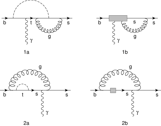
Figure 1: Examples of the correspondence between diagrams in the “full” theory and in the off-shell effective theory.

The use of an off-shell configuration induces in the result for the “full” theory the appearance of terms that behave as $1/m_{s}^{2}$, $1/m_{b}^{2}$, $\log\,m_{s}^{2}$, $\log\,m_{b}^{2}$ as $m_{s},\,m_{b}\rightarrow 0$. However, the effective theory has the same infrared behaviour and there is a one-to-one correspondence between $m_{s},\,m_{b}\rightarrow 0$ divergent contributions in the diagrams of the “full” and those of the effective theory. It is worth reminding that this correspondence works in the off-shell operator basis of eq. (4). In particular, diagrams like (1a) in fig. 1 have a counterpart in the effective theory, depicted in (1b), that requires the introduction of a $b\rightarrow sg\gamma$ vertex. Such a vertex is indeed present in the operators $Q_{9},\,Q_{10},\,Q_{12},\,Q_{13}$ while it does not appear in the on-shell operator basis. The corresponding contribution can be worked out either through the use of the Ward identities that relate the 1PI $b\rightarrow s\gamma$, $b\rightarrow sg$ vertex to the $b\rightarrow sg\gamma$ one [31], or by direct computation of the Feynman rules from the relevant operators. In an analogous way, topology (2a) requires a $b\to s$ transition vertex in the effective theory. The leading behaviour of (2a) as $m_{s},m_{b}\rightarrow 0$ is ${\cal O}(1/m_{s}^{2})$, ${\cal O}(1/m_{b}^{2})$ and this is eliminated if the “full” theory is renormalized on-shell [25] (see discussion in point 3 of section 2). Alternatively, if the vanishing of the off-diagonal mass terms is not enforced, then the introduction of the dimension-four operators [19]

$$\begin{array}[]{rl}M_{1}=&\frac{i}{16\pi^{2}}\,\bar{s}_{L}\not\!\!D\,b_{L},\vspace{0.2cm}\\ M_{2}=&\frac{1}{16\pi^{2}}m_{b}\,\bar{s}_{L}\,b_{R},\end{array}$$ (15)

in the diagram (2b) will provide such a cancellation. However, topology (2a) also shows an infrared logarithmic behaviour in the light quark masses. This cannot be eliminated through renormalization but it is actually cancelled when the operators $Q_{9}$ and $Q_{12}$ are inserted in diagram (2b).

It should be noticed that the cancellation of infrared $m_{s},\,m_{b}$ contributions between “full” and effective theory works before enforcing the GIM mechanism. Therefore the charm diagrams do not present any additional difficulty. The charm contribution to $C_{7_{OS}}$ can be obtained by replacing $m_{t}$ with $m_{c}$ and taking the limit $m_{c}\rightarrow 0$. After performing this operation one is left with some $\log\,m_{c}$ terms. However, the effective theory contains also the contribution of the operator $Q_{2}$ that provides the cancellation of these logarithmic terms through two-loop diagrams.

As already said, the procedure for extracting $C_{8_{OS}}$ is completely analogous, the only difference being that instead of introducing a $b\rightarrow sg\gamma$ vertex, one needs a $b\rightarrow sgg$ vertex. This is present in the operators $Q_{8},\,Q_{9},\,Q_{12},\,Q_{13},\,Q_{14}$. Again, the infrared divergent contributions associated with the gluon cancel diagram by diagram between the “full” and the effective theory.

4 Standard Model Results

In this section we present the result for the SM. The analysis is performed in the on-shell basis obtained by applying the EOM to the operators $Q_{9}\!-\!Q_{14}$. All the Wilson coefficients are now intended in the on-shell basis, but for simplicity we drop the subscript $OS$. The NLO expression for the branching ratio of the inclusive radiative decay $B\to X_{s}\gamma$ has been presented in ref. [13]:

$$BR_{\gamma}\equiv BR(B\to X_{s}\gamma) =BR(B\to X_{c}e\bar{\nu}_{e})\left|\frac{V_{ts}^{*}V_{tb}}{V_{cb}}\right|^{2}\frac{6\alpha_{e}}{\pi f(z)\kappa(z)}\frac{\bar{m}_{b}^{2}(\mu_{b})}{m_{b}^{2}}$$ (16)

$$\times\left(|D|^{2}+A\right)\left(1-\frac{\delta^{NP}_{SL}}{m_{b}^{2}}+\frac{\delta^{NP}_{\gamma}}{m_{b}^{2}}+\frac{\delta^{NP}_{c}}{m_{c}^{2}}\right)~{}.$$

Here and throughout the paper $m_{q}$ ($q=c,b,t$) denotes the quark pole mass, while ${\bar{m}}_{q}$ denotes the $\overline{MS}$ running mass,

$$\bar{m}_{q}(m_{q})=m_{q}\left[1-\frac{4}{3}\frac{\alpha_{s}(m_{q})}{\pi}\right]~{}.$$ (17)

Also $z=m_{c}^{2}/m_{b}^{2}$ and $f(z)$ and $\kappa(z)$ are the phase-space factor and the QCD correction [32] for the semileptonic decay,

$$\kappa(z)=1-\frac{2\alpha_{s}(\bar{\mu}_{b})}{3\pi}\frac{h(z)}{f(z)}$$ (18)

$$f(z)=1-8z+8z^{3}-z^{4}-12z^{2}\ln z$$ (19)

$$h(z)=-(1-z^{2})\left(\frac{25}{4}-\frac{239}{3}z+\frac{25}{4}z^{2}\right)+z\ln z\left(20+90z-\frac{4}{3}z^{2}+\frac{17}{3}z^{3}\right)$$

$$+z^{2}\ln^{2}z\;(36+z^{2})+(1-z^{2})\left(\frac{17}{3}-\frac{64}{3}z+\frac{17}{3}z^{2}\right)\ln(1-z)$$

$$-4(1+30z^{2}+z^{4})\ln z\;\ln(1-z)-(1+16z^{2}+z^{4})\left[6{\rm Li}_{2}(z)-\pi^{2}\right]$$

$$-32z^{3/2}(1+z)\left[\pi^{2}-4{\rm Li}_{2}(\sqrt{z})+4{\rm Li}_{2}(-\sqrt{z})-2\ln z\;\ln\left(\frac{1-\sqrt{z}}{1+\sqrt{z}}\right)\right].$$ (20)

In eq. (18) $\bar{\mu}_{b}$ is the renormalization scale relevant to the semileptonic process, a priori different than the renormalization scale relevant to the radiative decay, as stressed in ref. [14].

In order to relate the quark decay rate to the actual hadronic process, we have included the corrections obtained with the method of the Heavy-Quark Effective Theory (HQET), for a review, see e.g. ref. [33]. In terms of the contributions to a heavy hadron mass from kinetic energy ($\lambda_{1}$) and chromo-magnetic interactions ($\lambda_{2}$), the $1/m_{b}^{2}$ corrections to the semileptonic and radiative decays are

$$\delta_{SL}^{NP}=\frac{\lambda_{1}}{2}+\frac{3}{2}\lambda_{2}\left[1-4\frac{(1-z)^{4}}{f(z)}\right]~{},$$ (21)

$$\delta_{\gamma}^{NP}=\frac{\lambda_{1}}{2}-\frac{9}{2}\lambda_{2}~{}.$$ (22)

Notice that the dependence on the poorly-known parameter $\lambda_{1}$ drops out in eq. (16). We take $\lambda_{2}=(m_{B^{*}}^{2}-m_{B}^{2})/4=0.12$ GeV², as extracted from B-meson mass splitting. Voloshin [5] has considered also $1/m_{c}^{2}$ non-perturbative corrections coming from interference between the operators $O_{2}$ and $O_{7}$. With the correct sign found in ref. [6], these are given by

$$\delta_{c}^{NP}=-\frac{1}{9}\frac{\lambda_{2}}{C^{(0)}_{7}}\left(C^{(0)}_{2}-\frac{C^{(0)}_{1}}{6}\right)~{},$$ (23)

where $C^{(0)}_{2}$ and $C^{(0)}_{7}$ are the corresponding Wilson coefficients at the LO computed at the scale $\mu_{b}$. It appears that higher-order terms in $1/m_{c}^{2}$ are suppressed [7], and therefore non-perturbative corrections are presumably under control.

In eq. (16), $A$ is the correction coming from the bremsstrahlung process $b\to s\gamma g$, with a cutoff on the photon energy $E_{\gamma}>(1-\delta)m_{b}/2$ [11, 34],

$$A = \left(e^{-\alpha_{s}(\mu_{b})\ln\delta(7+2\ln\delta)/3\pi}-1\right)|C_{7}^{(0)eff}(\mu_{b})|^{2}$$ (24)

$$+\frac{\alpha_{s}(\mu_{b})}{\pi}\sum_{\stackrel{{\scriptstyle i,j=1}}{{i\leq j}}}^{8}C_{i}^{(0)eff}(\mu_{b})C_{j}^{(0)eff}(\mu_{b})f_{ij}(\delta).$$

The coefficients $f_{ij}(\delta)$, which have been computed in ref. [11, 34], are defined as in ref. [13]. To conform to previous literature, we define a “total” inclusive decay by choosing $\delta=0.99$, although for comparison we will also present results for $\delta=0.90$. The numerical values of the coefficients $f_{ij}(\delta)$, for $\delta=0.99$ and $\sqrt{z}=0.29$, are

$$f_{ij}=\pmatrix{0.0009&-0.0113&-0.0035&0.0006&-0.0459&-0.0600&-0.0030&0.0010\cr&0.0340&0.0210&-0.0035&0.2754&0.3599&0.0182&-0.0061\cr&&0.0140&-0.0047&0.3277&0.0666&0.0421&-0.0140\cr&&&0.0088&-0.0546&0.1570&-0.0070&0.0023\cr&&&&1.9369&0.9506&0.5926&-0.1975\cr&&&&&0.9305&0.0002&-0.0001\cr&&&&&&3.4211&0.3897\cr&&&&&&&3.2162}$$ (25)

Finally

$$D=C_{7}^{(0)eff}(\mu_{b})+\frac{\alpha_{s}(\mu_{b})}{4\pi}\left\{C_{7}^{(1)eff}(\mu_{b})+\sum_{i=1}^{8}C_{i}^{(0)eff}(\mu_{b})\left[r_{i}+\gamma_{i7}^{(0)eff}\ln\frac{m_{b}}{\mu_{b}}\right]\right\}~{}.$$ (26)

The coefficients $r_{i}$, obtained from an NLO matrix element calculation, have been calculated in ref. [12] for $i=1,2,7,8$. They can be found in ref. [13], together with the corresponding values of $\gamma_{i7}^{(0)eff}$. The dependence on $\mu_{b}$, the renormalization scale relevant for the $B\to X_{s}\gamma$ process, cancels out in $D$ at the leading order in $\alpha_{s}$. The relations between the Wilson coefficients at the low-energy scale $\mu_{b}$ and the high-energy scale $\mu_{\scriptscriptstyle W}$, obtained by renormalization group evolution, can be found in refs. [13, 14]. We are interested here in the expressions of the Wilson coefficients at the scale $\mu_{\scriptscriptstyle W}$, at which the “full” theory is matched into an effective theory with five quark flavours. In the SM model, they are given by

$$C^{eff}_{i}(\mu_{\scriptscriptstyle W})=C^{(0)eff}_{i}(\mu_{\scriptscriptstyle W})+\frac{\alpha_{s}(\mu_{\scriptscriptstyle W})}{4\pi}C^{(1)eff}_{i}(\mu_{\scriptscriptstyle W})$$ (27)

$$C_{i}^{(0)eff}(\mu_{\scriptscriptstyle W})=C_{i}^{(0)}(\mu_{\scriptscriptstyle W})=\left\{\begin{array}[]{cc}0&\mbox{ for $i=1,3,4,5,6$}\\ 1&\mbox{ for $i=2$}\\ \vspace{0.2cm}F_{i}^{(1)}(x)&\mbox{ for $i=7,8$},\\ \end{array}\right.$$ (28)

$$F_{7}^{(1)}(x)=\frac{x(7-5x-8x^{2})}{24(x-1)^{3}}+\frac{x^{2}(3x-2)}{4(x-1)^{4}}\ln x$$ (29)

$$F_{8}^{(1)}(x)=\frac{x(2+5x-x^{2})}{8(x-1)^{3}}-\frac{3x^{2}}{4(x-1)^{4}}\ln x$$ (30)

$$x=\frac{\bar{m}_{t}^{2}(\mu_{\scriptscriptstyle W})}{M_{\scriptscriptstyle W}^{2}}.$$ (31)

The NLO top-quark running mass at the scale $\mu_{\scriptscriptstyle W}$ is given by

$$\bar{m}_{t}(\mu_{\scriptscriptstyle W})=\bar{m}_{t}(m_{t})\left[\frac{\alpha_{s}(\mu_{\scriptscriptstyle W})}{\alpha_{s}(m_{t})}\right]^{\frac{\gamma_{0}^{m}}{2\beta_{0}}}\left[1+\frac{\alpha_{s}(m_{t})}{4\pi}\frac{\gamma_{0}^{m}}{2\beta_{0}}\left(\frac{\gamma_{1}^{m}}{\gamma_{0}^{m}}-\frac{\beta_{1}}{\beta_{0}}\right)\left(\frac{\alpha_{s}(\mu_{\scriptscriptstyle W})}{\alpha_{s}(m_{t})}-1\right)\right]~{},$$ (32)

$$\beta_{0}=11-\frac{2}{3}n_{f}~{},~{}~{}~{}~{}\beta_{1}=102-\frac{38}{3}n_{f}~{},$$ (33)

$$\gamma_{0}^{m}=8~{},~{}~{}~{}~{}\gamma_{1}^{m}=\frac{404}{3}-\frac{40}{9}n_{f}~{},$$ (34)

and it is related to the pole mass by eq. (17). Here $n_{f}$ is the effective number of quark flavours. We have computed the NLO corrections using the method illustrated in sect. 3 and confirmed the results of ref. [10]

$$C_{i}^{(1)eff}(\mu_{\scriptscriptstyle W})=\left\{\begin{array}[]{cc}15+6\ln\frac{\mu_{\scriptscriptstyle W}^{2}}{M_{\scriptscriptstyle W}^{2}}&\mbox{ for $i=1$}\\ 0&\mbox{ for $i=2,3,5,6$}\\ E(x)-\frac{2}{3}+\frac{2}{3}\ln\frac{\mu_{\scriptscriptstyle W}^{2}}{M_{\scriptscriptstyle W}^{2}}&\mbox{ for $i=4$}\\ G_{i}(x)+\Delta_{i}(x)\ln\frac{\mu_{\scriptscriptstyle W}^{2}}{M_{\scriptscriptstyle W}^{2}}&\mbox{for $i=7,8$},\end{array}\right.$$ (35)

$$E(x)=\frac{x(-18+11x+x^{2})}{12(x-1)^{3}}+\frac{x^{2}(15-16x+4x^{2})}{6(x-1)^{4}}\ln x-\frac{2}{3}\ln x.$$ (36)

$$G_{7}(x) = \frac{-16x^{4}-122x^{3}+80x^{2}-8x}{9(x-1)^{4}}{\rm Li}_{2}\left(1-\frac{1}{x}\right)+\frac{6x^{4}+46x^{3}-28x^{2}}{3(x-1)^{5}}\ln^{2}x$$ (37)

$$+\frac{-102x^{5}-588x^{4}-2262x^{3}+3244x^{2}-1364x+208}{81(x-1)^{5}}\ln x$$

$$+\frac{1646x^{4}+12205x^{3}-10740x^{2}+2509x-436}{486(x-1)^{4}}\vspace{0.2cm}$$

$$G_{8}(x) = \frac{-4x^{4}+40x^{3}+41x^{2}+x}{6(x-1)^{4}}{\rm Li}_{2}\left(1-\frac{1}{x}\right)+\frac{-17x^{3}-31x^{2}}{2(x-1)^{5}}\ln^{2}x$$ (38)

$$+\frac{-210x^{5}+1086x^{4}+4893x^{3}+2857x^{2}-1994x+280}{216(x-1)^{5}}\ln x$$

$$+\frac{737x^{4}-14102x^{3}-28209x^{2}+610x-508}{1296(x-1)^{4}}$$

$$\Delta_{7}(x)=\frac{208-1111x+1086x^{2}+383x^{3}+82x^{4}}{81(x-1)^{4}}+\frac{2x^{2}(14-23x-3x^{2})}{3(x-1)^{5}}\ln x$$ (39)

$$\Delta_{8}(x)=\frac{140-902x-1509x^{2}-398x^{3}+77x^{4}}{108(x-1)^{4}}+\frac{x^{2}(31+17x)}{2(x-1)^{5}}\ln x$$ (40)

The $\mu_{\scriptscriptstyle W}$ dependence in all terms of order $\alpha_{s}$ in eq. (26) cancels out because eqs. (39) and (40) satisfy the relation

$$\Delta_{i}=\gamma_{0}^{m}x\frac{\partial C_{i}^{(0)}}{\partial x}+\frac{1}{2}\sum_{j=1}^{8}\gamma_{ji}^{(0)eff}C_{j}^{(0)}$$ (41)

$\mu_{b}$	$\bar{\mu}_{b}$	$\mu_{\scriptscriptstyle W}$	$m_{t}$	${}_{\left|\frac{V_{tb}V^{\star}_{ts}}{V_{cb}}\right|^{2}}$	$m_{c}/m_{b}$	$m_{b}-m_{c}$	$BR_{SL}$	$\alpha_{s}(M_{Z})$	$\alpha_{e}^{-1}$
[GeV]	[GeV]	[GeV]	[GeV]			[GeV]
Central values
4.8	4.8	80.33	175	0.95	0.29	3.39	0.1049	0.118	130.3
Errors/Ranges
${}^{+4.8}_{-2.4}$	${}^{+4.8}_{-2.4}$	${}^{+80.33}_{-40.16}$	$\pm 5$	$\pm 0.03$	$\pm 0.02$	$\pm 0.04$	$\pm 0.0046$	$\pm 0.003$	$\pm 2.3$
Uncertainty in $BR_{\gamma}$ (LO)
${}_{+24}^{-19}\%$	-	${}^{+9.3}_{-9.7}\%$	$\pm 1.6\%$	$\pm 3.2\%$	${}^{+8.5}_{-7.3}\%$	${}^{-0.07}_{+0.08}\%$	$\pm 4.4\%$	${}^{+2.3}_{-2.2}\%$	${}^{-1.7}_{+1.8}\%$
Uncertainty in $BR_{\gamma}$ (NLO)
${}^{+0.0}_{-3.5}\%$	${}^{-1.4}_{+2.1}$	${}^{-1.1}_{+2.1}\%$	$\pm 1.4\%$	$\pm 3.2\%$	${}^{+4.5}_{-3.8}\%$	$\mp 0.4\%$	$\pm 4.4\%$	${}^{+2.9}_{-2.8}\%$	${}^{-1.7}_{+1.8}\%$

Table 1: The input parameters entering the calculation of $BR_{\gamma}$, their central values, their errors, their influence on the uncertainty in $BR_{\gamma}$ at the LO and NLO. The other constants entering the calculation are $M_{\scriptscriptstyle W}=80.33$ GeV, $\lambda_{2}=0.12$ GeV², $m_{s}/m_{b}=50$, and $\delta=0.99$.

The values of the parameters chosen in our numerical analysis are shown in table 1. The value of $\alpha_{s}(M_{Z})$, obtained from an average of low- and high-energy measurements, is taken from ref. [36]. From this we calculate $\alpha_{s}$ at a generic scale $\mu$ with the NLO result

$$\alpha_{s}(\mu)=\frac{\alpha_{s}(M_{Z})}{v}\left(1-\frac{\beta_{1}}{\beta_{0}}\frac{\alpha_{s}(M_{Z})}{4\pi}\frac{\ln v}{v}\right)~{}~{}~{}~{}~{}v=1+\beta_{0}\frac{\alpha_{s}(M_{Z})}{2\pi}\ln\frac{\mu}{M_{Z}}~{}.$$ (42)

The top quark mass is obtained by combining the results by CDF [37] ($m_{t}=176.8\pm 4.4^{stat}\pm 4.8^{syst}$ GeV) and D0 [38] ($m_{t}=173.3\pm 5.6^{stat}\pm 6.2^{syst}$ GeV). The difference between the bottom and charm mass is obtained from the HQET relation between the quark and hadron masses, $m_{b}-m_{c}=3.39\pm 0.03\pm 0.03$ GeV [39], where the first error is from the uncertainty in $\lambda_{1}$ and the second one from higher-order corrections. The ratio $m_{c}/m_{b}$ is chosen in the range $0.29\pm 0.02$, which corresponds to $m_{b}=4.77\pm 0.15$ GeV.

The uncertainty on the electromagnetic coupling $\alpha_{e}$ corresponds to the arbitrariness of choosing the renormalization scale between $m_{b}$ and $M_{\scriptscriptstyle W}$, as QED corrections have not been included.

The experimental situation on the semileptonic branching ratio $BR_{SL}$ is rather controversial (for a review, see ref. [40]). The two measurements at the $\Upsilon(4S)$ give $BR_{SL}=(10.49\pm 0.17\pm 0.43)$% (CLEO [41]) and $BR_{SL}=(9.7\pm 0.5\pm 0.4)$% (ARGUS [42]). On the other hand, the average of the four LEP experiments gives [43, 44] $BR_{SL}^{Z}=(10.95\pm 0.13\pm 0.29)$%. However the $B$ samples at the $Z^{0}$ also contain $B$ hadrons which have typically shorter lifetimes than $B$ mesons. Following Neubert [39], we can correct $BR_{SL}^{Z}$ using the average lifetime of the corresponding $B$ mixture and obtain $BR_{SL}=(11.23\pm 0.34)\%$ at $Z^{0}$. The low- and high-energy results show a certain discrepancy. However, a reanalysis of the LEP results is finding new systematic errors and a new dedicated analysis is in progress [44]. For this reason we prefer to use only the CLEO result.

In terms of the Wolfenstein parameters $\lambda$, $\rho$, and $\eta$ related to the standard parametrisation [36] by

$$s_{12}=\lambda,~{}~{}~{}\frac{s_{13}e^{-i\delta}}{s_{23}}=\lambda(\rho-i\eta)$$ (43)

and using unitarity, the relevant CKM factor can be written as

$$\left|\frac{V_{ts}^{*}V_{tb}}{V_{cb}}\right|^{2}=1+(2\rho-1)\lambda^{2}~{}.$$ (44)

For $\lambda=0.221$ and $\rho$ in the range between $-0.3$ and 0.3, we obtain the value shown in table 1. The new physics contributions that we will consider in sect. 5 can modify the values of $\rho$ obtained from fits of different flavour-physics measurements. However, since we allow a rather large range for $\rho$, these effects are included in the error.

To estimate higher-order effects, we vary the different renormalization scales $\mu_{b}$, $\bar{\mu}_{b}$, and $\mu_{\scriptscriptstyle W}$ in the ranges given in table 1, which correspond to shifts in the logarithms of the scale by an amount $\pm\ln 2$ around their central values $\mu_{b}=\bar{\mu}_{b}=m_{b}$, $\mu_{\scriptscriptstyle W}=M_{\scriptscriptstyle W}$. In the NLO calculation we have dropped all explicit ${\cal O}(\alpha_{s}^{2})$ terms in eq. (16). To allow a better comparison, we also perform the calculation in LO approximation, where ${\cal O}(\alpha_{s})$ terms are set to zero and $\alpha_{s}$ is evolved using the one-loop renormalization group equation.

The result of the numerical evaluation of eq. (16) is

$$BR_{\gamma}=(2.66\pm 0.74)\times 10^{-4}~{}~{}~{}({\rm LO})$$ (45)

$$BR_{\gamma} = (3.62\pm 0.33)\times 10^{-4}~{}~{}~{}({\rm NLO},\delta=0.99)$$ (46)

$$(3.54\pm 0.32)\times 10^{-4}~{}~{}~{}({\rm NLO},\delta=0.90)$$

The error is obtained by adding in quadratures the errors due to the different input parameters shown in table 1. If the error is asymmetric, we always choose the larger uncertainty. The $\mu_{b}$ scale dependence dominates the error at the LO, but it is drastically reduced at the NLO. This is illustrated in fig. 2. The result in eq. (46) is in agreement with those presented in refs. [13, 14]. The slightly different $\mu_{b}$ dependence we are finding comes from our choice of defining $\bar{m}_{b}$ in eq. (16) at the scale $\mu_{b}$ (where the operator $Q_{7}$ is defined), instead of $m_{b}$ as in refs. [13, 14]. Of course this just corresponds to a higher-order effect, and this ambiguity is taken into account by the theoretical uncertainty.

Given the controversial situation in $BR_{SL}$, it is useful to quote also the prediction for the ratio $BR_{\gamma}/BR_{SL}$ (for $\delta=0.99$)

$$BR_{\gamma}/BR_{SL}=(2.54\pm 0.70)\times 10^{-3}~{}~{}~{}({\rm LO})$$ (47)

$$BR_{\gamma}/BR_{SL}=(3.45\pm 0.27)\times 10^{-3}~{}~{}~{}({\rm NLO})$$ (48)

Figure 2: The $\mu_{b}$ scale dependence of $BR_{\gamma}(\delta=0.99)$ at LO (lower curves) and NLO (upper curves). The solid line represents the case in which all input parameters are fixed to their central values. The dashed lines represent the errors coming from all input parameters, other than $\mu_{b}$, added in quadratures.

5 Two-Higgs Doublet Models

In this section we investigate the prediction for $BR_{\gamma}$ in models with two Higgs doublets. The new ingredient with respect to the SM is the presence of a charged Higgs scalar particle which gives new contributions to the Wilson coefficients of the effective theory. The interaction between quarks and the charged Higgs $H^{\pm}$ is defined by the Lagrangian

$${\cal L}=(2\sqrt{2}G_{F})^{1/2}\sum_{i,j=1}^{3}\bar{u}_{i}\left(A_{u}m_{u_{i}}V_{ij}\frac{1-\gamma_{5}}{2}-A_{d}V_{ij}m_{d_{i}}\frac{1+\gamma_{5}}{2}\right)d_{j}H^{+}+{\rm h.c.}$$ (49)

Here $i,j$ are generation indices, $m_{u,d}$ are quark masses, and $V$ is the CKM matrix. We are considering only models in which FCNCs vanish at tree level [45]. Therefore we have two possibilities which are parametrised by the model-dependent coefficients $A_{u}$ and $A_{d}$. The first possibility, referred to as Model I, is that both up and down quarks get their masses from the same Higgs doublet $H_{2}$, and

$$A_{u}=A_{d}=1/\tan\beta~{},$$ (50)

where $\tan\beta=\langle H_{2}^{0}\rangle/\langle H_{1}^{0}\rangle$. The case of Model II is that up quarks get their masses from Yukawa couplings to $H_{2}$, while down quarks get masses from couplings to $H_{1}$, and

$$A_{u}=-1/A_{d}=1/\tan\beta~{}.$$ (51)

The latter case is particularly interesting because it is realized in the minimal supersymmetric extension of the SM.

In the language of the effective theory, it is easy to include the charged-Higgs effect. We just need to compute the new Wilson coefficients at the matching scale $\mu_{\scriptscriptstyle W}$, since they contain all the relevant ultraviolet information. At the LO, the charged-Higgs contribution, to be added to eq. (28) is given by [46]

$$\delta C_{i}^{(0)eff}(\mu_{\scriptscriptstyle W})=0~{}~{}~{}~{}~{}i=1,...,6$$ (52)

$$\delta C_{7,8}^{(0)eff}(\mu_{\scriptscriptstyle W})=\frac{A_{u}^{2}}{3}F_{7,8}^{(1)}(y)-A_{u}A_{d}F_{7,8}^{(2)}(y)$$ (53)

$$F_{7}^{(2)}(y)=\frac{y(3-5y)}{12(y-1)^{2}}+\frac{y(3y-2)}{6(y-1)^{3}}\ln y$$ (54)

$$F_{8}^{(2)}(y)=\frac{y(3-y)}{4(y-1)^{2}}-\frac{y}{2(y-1)^{3}}\ln y$$ (55)

$$y=\frac{\bar{m}_{t}^{2}(\mu_{\scriptscriptstyle W})}{M_{H}^{2}}~{},$$ (56)

and $F_{7,8}^{(1)}$ are defined in eqs. (29)–(30).

At the NLO, the charged-Higgs contributions to the Wilson coefficients are

$$\delta C_{i}^{(1)eff}(\mu_{\scriptscriptstyle W})=0~{}~{}~{}~{}~{}i=1,2,3,5,6$$ (57)

$$\delta C_{4}^{(1)eff}(\mu_{\scriptscriptstyle W})=E^{H}(y)$$ (58)

$$\delta C_{7}^{(1)eff}(\mu_{\scriptscriptstyle W}) = G_{7}^{H}(y)+\Delta_{7}^{H}(y)\ln\frac{\mu_{\scriptscriptstyle W}^{2}}{M_{H}^{2}}-\frac{4}{9}E^{H}(y)$$

$$\delta C_{8}^{(1)eff}(\mu_{\scriptscriptstyle W}) = G_{8}^{H}(y)+\Delta_{8}^{H}(y)\ln\frac{\mu_{\scriptscriptstyle W}^{2}}{M_{H}^{2}}-\frac{1}{6}E^{H}(y)$$ (59)

with

$$G_{7}^{H}(y) = A_{d}A_{u}\frac{4}{3}y\left[\frac{4(-3+7y-2y^{2})}{3(y-1)^{3}}{\rm Li}_{2}\left(1-\frac{1}{y}\right)+\frac{8-14y-3y^{2}}{3(y-1)^{4}}\ln^{2}y\right.$$ (60)

$$\left.+\frac{2(-3-y+12y^{2}-2y^{3})}{3(y-1)^{4}}\ln y+\frac{7-13y+2y^{2}}{(y-1)^{3}}\right]$$

$$+A^{2}_{u}\frac{2}{9}y\left[\frac{y(18-37y+8y^{2})}{(y-1)^{4}}{\rm Li}_{2}\left(1-\frac{1}{y}\right)+\frac{y(-14+23y+3y^{2})}{(y-1)^{5}}\ln^{2}y\right.$$

$$+\frac{-50+251y-174y^{2}-192y^{3}+21y^{4}}{9(y-1)^{5}}\ln y$$

$$\left.+\frac{797-5436y+7569y^{2}-1202y^{3}}{108(y-1)^{4}}\right]$$

$$\Delta_{7}^{H}(y) = A_{d}A_{u}\frac{2}{9}y\left[\frac{21-47y+8y^{2}}{(y-1)^{3}}+\frac{2(-8+14y+3y^{2})}{(y-1)^{4}}\ln y\right]$$ (61)

$$+A_{u}^{2}\frac{2}{9}y\left[\frac{-31-18y+135y^{2}-14y^{3}}{6(y-1)^{4}}+\frac{y(14-23y-3y^{2})}{(y-1)^{5}}\ln y\right]$$

$$G_{8}^{H}(y) = A_{d}A_{u}\frac{1}{3}y\left[\frac{-36+25y-17y^{2})}{2(y-1)^{3}}{\rm Li}_{2}\left(1-\frac{1}{y}\right)+\frac{19+17y}{(y-1)^{4}}\ln^{2}y\right.$$ (62)

$$\left.+\frac{-3-187y+12y^{2}-14y^{3})}{4(y-1)^{4}}\ln y+\frac{3(143-44y+29y^{2})}{8(y-1)^{3}}\right]$$

$$+A^{2}_{u}\frac{1}{6}y\left[\frac{y(30-17y+13y^{2})}{(y-1)^{4}}{\rm Li}_{2}\left(1-\frac{1}{y}\right)-\frac{y(31+17y)}{(y-1)^{5}}\ln^{2}y\right.$$

$$+\frac{-226+817y+1353y^{2}+318y^{3}+42y^{4}}{36(y-1)^{5}}\ln y$$

$$\left.+\frac{1130-18153y+7650y^{2}-4451y^{3}}{216(y-1)^{4}}\right]$$

$$\Delta_{8}^{H}(y) = A_{d}A_{u}\frac{1}{3}y\left[\frac{81-16y+7y^{2}}{2(y-1)^{3}}-\frac{19+17y}{(y-1)^{4}}\ln y\right]$$ (63)

$$+A_{u}^{2}\frac{1}{6}y\left[\frac{-38-261y+18y^{2}-7y^{3}}{6(y-1)^{4}}+\frac{y(31+17y)}{(y-1)^{5}}\ln y\right]$$

$$E^{H}(y)=A_{u}^{2}\left[\frac{y(16-29y+7y^{2})}{36(y-1)^{3}}+\frac{y(3y-2)}{6(y-1)^{4}}\ln y\right]~{}.$$ (64)

The $\mu_{\scriptscriptstyle W}$ dependence cancels in terms of ${\cal O}(\alpha_{s})$, since the $H^{\pm}$ contribution satisfies eq. (41).

Figure 3: Predicted $BR_{\gamma}(\delta=0.99)$ in Model II as a function of the charged-Higgs mass $M_{H}$, for $\tan\beta=2$ at LO (solid line). The dashed lines represent the uncertainty obtained by adding in quadratures the errors coming from the different input parameters. The dot-dashed lines define the uncertainty range with the “scanning” method (see text).

Figure 4: Predicted $BR_{\gamma}(\delta=0.99)$ in Model II as a function of the charged-Higgs mass $M_{H}$, for $\tan\beta=2$ at NLO (solid line). The dashed lines represent the uncertainty obtained by adding in quadratures the errors coming from the different input parameters. The dot-dashed lines define the uncertainty range with the “scanning” method (see text).

In figs. 3 and 4 we show the predicted value of $BR_{\gamma}$ in Model II as a function of the charged-Higgs mass $M_{H}$, for $\tan\beta=2$ at LO and NLO with $\delta=0.99$. As apparent from these figures, the decoupling at large $M_{H}$ occurs very slowly. Moreover, the $H^{\pm}$ contribution always increases the SM value of $BR_{\gamma}$. Since the SM prediction is already quite higher than the CLEO measurement, one can obtain very stringent bounds on $M_{H}$ [47]. These bounds are very sensitive on the errors of the theoretical prediction. Improving the calculation to the NLO has important effects on these bounds, since the theoretical error is significantly reduced, as shown in figs. 3 and 4.

Because of the large sensitivity on errors, we will use two different methods to define the bounds on $M_{H}$. We define a “Gaussian” standard deviation by adding different input errors in quadratures. We also define a “scanning” method of estimating errors by varying independently all input parameters within the ranges defined in table 1. Figures 3 and 4 show the errors on the theoretical prediction using one “Gaussian” standard deviation (dashed lines), or using the “scanning” method (dot-dashed lines). If we apply the “scanning” method to the SM, we obtain (for $\delta=0.99$)

$$BR_{\gamma}=(2.66^{+1.78}_{-1.09})\times 10^{-4}~{}~{}~{}({\rm LO})$$ (65)

$$BR_{\gamma}=(3.62^{+0.92}_{-0.77})\times 10^{-4}~{}~{}~{}({\rm NLO})$$ (66)

$$BR_{\gamma}/BR_{SL}=(2.54^{+1.52}_{-0.97})\times 10^{-3}~{}~{}~{}({\rm LO})$$ (67)

$$BR_{\gamma}/BR_{SL}=(3.45^{+0.69}_{-0.61})\times 10^{-3}~{}~{}~{}({\rm NLO})$$ (68)

This has to be compared with the “Gaussian” standard deviation error given in eqs. (45)–(48).

Figure 5: Exclusion regions in the plane $BR_{\gamma}/BR_{SL}$ versus $M_{H}$ for $\tan\beta=$ 1 (dashed lines), 2 (solid lines), 5 (dot-dashed lines) obtained by our NLO calculation with $\delta=0.90$. The upper lines correspond to a theoretical uncertainty defined by one “Gaussian” standard deviation, and the lower lines to the “scanning” method (see text).

Next, we exclude a value of $M_{H}$ if the minimum of $BR_{\gamma}$ inside the “Gaussian” (or “scanning”) band lies above the present CLEO 95% CL upper bound $BR_{\gamma}<4.2\times 10^{-4}$ [2]. The corresponding limits on $M_{H}$ are shown in table 2, for different values of $\tan\beta$. If we restrict our consideration to the case $\tan\beta>1$, the dependence on $\tan\beta$ is very mild, and the limit practically saturates for $\tan\beta\mathrel{\hbox to0.0pt{\raise 2.15277pt\hbox{$>$}\hss}{\lower 2.15277pt\hbox{$\sim$}}}2$. Notice that, for a “Gaussian” error, going from the LO to the NLO calculation allows an improvement of the limit on $M_{H}$ from about 260 GeV to about 370 GeV, for large $\tan\beta$, even in the more conservative case of $\delta=0.90$. Had we neglected the NLO Higgs matching condition, but kept the remaining NLO corrections (as done in ref. [48]), we would find a much stronger limit $M_{H}>460$ GeV ($\tan\beta=5$, “Gaussian” error).

$\tan\beta$	theor. error	$M_{H}$ (LO)	$M_{H}$ (NLO)	$M_{H}$ (NLO)
		[GeV]	[GeV]($\delta=0.99$)	[GeV] ($\delta=0.90$)
1	“Gaussian”	300	473	408
2	“Gaussian”	268	440	377
5	“Gaussian”	258	430	368
1	“scanning”	240	316	276
2	“scanning”	208	287	249
5	“scanning”	198	278	242

Table 2: Lower bounds on the charged-Higgs mass $M_{H}$ from the CLEO 95% CL limit $BR_{\gamma}<4.2\times 10^{-4}$, using LO or NLO calculations. The theoretical uncertainty is estimated either with one “Gaussian” standard deviation, with input parameter errors added in quadratures, or with the “scanning” method, by varying independently the input parameters within their range. The NLO results are presented for two different values of the cut on the photon energy $\delta$.

It may seem disturbing to integrate out the top quark, the $W$, and a charged Higgs as heavy as 300 GeV or more at the same scale $\mu_{\scriptscriptstyle W}$. However, since we have completed the NLO calculation, the residual dependence on $\mu_{\scriptscriptstyle W}$ is very small. A resummation of the leading logarithms of $M_{H}/m_{W}$ has been performed in ref. [49].

Figure 6: The ratio between $BR_{\gamma}(\delta=0.90)$ predicted in Model I and the SM value, for the minimum $\tan\beta$ allowed by the $R_{b}$ measurement (solid line), for $\tan\beta=2$ (dashed line) and $\tan\beta=3$ (dot-dashed line). The solid line is interrupted at $\tan\beta=1$.

Certainly one of the reasons we are able to obtain such strong bounds on $M_{H}$ is the poor agreement between SM prediction and CLEO measurement. In view of the preliminary ALEPH result on $BR_{\gamma}$ and the controversial situation on $BR_{SL}$, it is more appropriate to present our results in a fashion which is independent of the present measurements. This is done in fig. 5, which shows the bound on $M_{H}$ according to the “Gaussian” and “scanning” methods, for any given value of the experimental upper bound on $BR_{\gamma}/BR_{SL}$ in the more conservative case $\delta=0.90$. The region below the curves is excluded by our theoretical calculation. As future measurements on $BR_{\gamma}/BR_{SL}$ improve, on can simply read off the limit on $M_{H}$ from the lines of fig. 5.

It should be remarked that, although Model II corresponds to the supersymmetric Higgs sector, these bounds do not directly apply to the supersymmetric extension of the SM. The reason is that contributions coming from other new particles can partly compensate the effect of the charged Higgs. In particular, in the supersymmetric limit, there is an exact cancellation of different contributions [50]. In the realistic case of broken supersymmetry, this cancellation is spoiled but, if charginos and stops are light, it may still be partially effective. Nevertheless, the bound presented here severely restricts the allowed region of parameter space.

In the case of Model I, the charged-Higgs contribution reduces the value of $BR_{\gamma}$ and therefore we cannot obtain any significant bound. On the other hand, it is interesting that new physics effects can bring the prediction for $BR_{\gamma}$ closer to the CLEO value.

A significant effect can only be expected for small $\tan\beta$, since in Model I all charged-Higgs contributions vanish in the limit of large $\tan\beta$, as $\tan^{-2}\beta$. When $\tan\beta$ is reduced, the top Yukawa coupling grows, and one eventually is limited by new contributions to $R_{b}$, $B^{0}$-$\bar{B}^{0}$ mixing, and occurrence of a Landau pole at intermediate energies (see e.g. ref. [51]). We have checked that the strongest experimental lower bound on $\tan\beta$ comes from $R_{b}$, the ratio between the bottom and hadronic $Z^{0}$ widths. Using the 95% CL lower limit $R_{b}>0.2155$ obtained from a combined LEP+SLD analysis ($R_{b}=0.2170\pm 0.009$ [43]) and the smallest top-quark mass value inside our range ($m_{t}=170$ GeV), we derive a lower bound on $\tan\beta$ of 1.8, 1.4, 1.0 for $M_{H}=85$, 200, and 425 GeV, respectively. For these values of $\tan\beta$ and $M_{H}$, the $B^{0}$-$\bar{B}^{0}$ mixing parameter is increased by about 30% with respect to the SM. Such an increase is compatible with experiments, given that the theoretical uncertainty on the hadronic parameter $F_{B}^{2}B_{B}$ is at least 40%. In correspondence to this minimum value of $\tan\beta$ we obtain the maximum reduction factor of $BR_{\gamma}$ with respect to the SM value, plotted in fig. 6. This reduction can be at best about 20%. For comparison we also show the theoretical prediction on $BR_{\gamma}/(BR_{\gamma})_{SM}$ for different values of $\tan\beta$. The lines in fig. 6 correspond to the central values of the input parameters defined in table 1, and error effects have not been included.

6 Conclusions

We have presented the ${\cal O}(\alpha_{s})$ QCD corrections to the matching conditions of the flavour-violating magnetic and chromo-magnetic operators both in the SM and in two-Higgs doublet model. We have worked with an off-shell effective Hamiltonian, and this has allowed us to compute the relevant Feynman diagrams without the use of asymptotic expansions.

Following this different method we have confirmed the results for the matching conditions in the SM first found in ref. [10], and recently recomputed in refs. [16, 14]. Our numerical analysis for the branching ratio of $B\to X_{s}\gamma$ gives

$$BR_{\gamma}=(3.62\pm 0.33)\times 10^{-3}$$ (69)

in agreement with previous literature [13, 14].

We have then extended our results to the case of two-Higgs doublet models. In the case of Model II, the charged-Higgs contribution always increases the SM prediction. Since the present CLEO measurement lies below the SM result, $B\to X_{s}\gamma$ provides quite stringent bounds on the charged-Higgs mass $M_{H}$. These bounds are very sensitive to the theoretical errors. The improvement of the calculation to the NLO significantly reduces the theoretical uncertainty and therefore tightens considerably the $M_{H}$ bounds. Our results are summarised in fig. 5, which shows the region in the plane $BR_{\gamma}/BR_{SL}$ versus $M_{H}$ excluded by our theoretical calculation. An experimental upper bound on $BR_{\gamma}/BR_{SL}$ can then be easily translated into a bound on $M_{H}$. For instance, using the present CLEO experimental results and a theoretical uncertainty defined by one “Gaussian” standard deviation, we find that charged-Higgs masses below 370 GeV are excluded. This result improves the bound of about 260 GeV obtained by LO calculations. We recall that the experimental results for $BR_{SL}$ show a certain discrepancy between low- and high-energy measurements (as discussed in sect. 4) and the preliminary ALEPH result for $B\to X_{s}\gamma$ is not in perfect agreement with the CLEO measurements. As shown in fig. 5, developments in the experimental situation can have an important effect on the $M_{H}$ bounds.

This bound on $M_{H}$ does not directly apply to the case of supersymmetric models, since contributions from other new particles can compensate the charged Higgs effect, and this is indeed known to happen in certain cases [50]. Nevertheless, it is clear that this bound is so strong that it severely restricts the allowed parameter space. This has important consequences on the prediction of new particle masses and on their observability at future colliders. However, it has to be remarked once again that the impressive restrictiveness of our bound on $M_{H}$ is partly a consequence of the poor agreement between theory and the CLEO measurement. Developments on the experimental side or new understanding of non-perturbative effects may then partially relax this bound.

Finally we have investigated the Model I version of theories with two-Higgs doublets. In this case, the charged-Higgs contribution reduces the SM value for $BR_{\gamma}$. Therefore one cannot derive useful bounds on $M_{H}$, but instead the theoretical prediction can be brought closer to the CLEO measurement. However, in view of the limits on $R_{b}$, the Model I charged Higgs can reduce the SM prediction for $BR_{\gamma}$ by at most 20%.

We wish to thank  F. Borzumati,  P. Chankowski,  K. Chetyrkin,  C. Greub, M. Mangano, G. Martinelli, M. Misiak, M. Neubert, M. Testa, and C. Wagner for useful conversations and D. Schlatter and H. Wachsmuth for discussions of the experimental results. We also acknowledge useful communications with A. Buras, G. Isidori, and N. Pott. One of us (G.D.) would like to thank the Physics Department of New York University for the kind ospitality during the initial stage of this project.

Note added: The calculation of the matching condition of $Q_{7}$ for the two-Higgs doublet model II, in the large $\tan\beta$ limit, has also been recently presented in ref. [52], and the result agrees with our eq. (60). In the final version of this paper, various formulae entering the calculation of $BR(B\to X_{s}\gamma)$ have been corrected, following suggestions by F. Borzumati, C. Greub, M. Misiak and M. Neubert.

References

• [1] R. Ammar et al. (CLEO Collab.), Phys. Rev. Lett. 71 (1993) 674.
• [2] M.S. Alam et al. (CLEO Collab.), Phys. Rev. Lett. 74 (1995) 2885.
• [3] A.F. Falk, M. Luke, and M. Savage, Phys. Rev. D49 (1994) 3367.
• [4] N.G. Deshpande, X.-G. He, and J. Trampetic, Phys. Lett. B367 (1996) 362;
J.M. Soares, Phys. Rev. D53 (1996) 241;
G. Eilam, A. Ioanissian, R.R. Mendel, and P. Singer, Phys. Rev. D53 (1996) 3629.
• [5] M.B. Voloshin, Phys. Lett. B397 (1997) 295.
• [6] G. Buchalla, G. Isidori, and S.J. Rey, preprint hep-ph/9705253.
• [7] A. Khodjamirian, R. Rückl, G. Stoll, and D. Wyler, Phys. Lett. B402 (1997) 167;
Z. Ligeti, L. Randall, and M.B. Wise, Phys. Lett. B402 (1997) 178;
A.K. Grant, A.G. Morgan, S. Nussinov, and R.D. Peccei, Phys. Rev. D56 (1997) 3151.
• [8] A.J. Buras, M. Misiak, M. Münz and S. Pokorski, Nucl. Phys. B424 (1994) 374.
• [9] M. Ciuchini et al., Phys. Lett. B334 (1994) 137.
• [10] K. Adel and Y.P. Yao, Phys. Rev. D49 (1994) 4945.
• [11] A. Ali and C. Greub, Z. Phys. C49 (1991) 431; Phys. Lett. B259 (1991) 182; Z. Phys. C60 (1993) 433; Phys. Lett. B361 (1995) 146.
• [12] C. Greub, T. Hurth and D. Wyler, Phys. Lett. B380 (1996) 385; Phys. Rev. D54 (1996) 3350.
• [13] K. Chetyrkin, M. Misiak and M. Münz, Phys. Lett. B400 (1997) 206.
• [14] A.J. Buras, A. Kwiatkowski and N. Pott, preprint TUM-HEP-287-97 [hep-ph/9707482].
• [15] F. Parodi, talk presented at the 32nd Rencontres de Moriond, March 1997.
• [16] C. Greub and T. Hurth, Phys. Rev. D56 (1997) 2934.
• [17] See V.A. Smirnov, Mod. Phys. Lett. A10 (1995) 1485 and references therein.
• [18] G. Cella, G .Curci, G. Ricciardi and A. Viceré, Nucl. Phys. B431 (1994) 417.
• [19] H. Simma, Z. Phys. C61 (1994) 67.
• [20] K. Wilson, Phys. Rev. D179 (1969) 1499.
• [21] E. Witten, Nucl. Phys. B122 (1977) 109.
• [22] L.F. Abbott, Nucl. Phys. B185 (1981) 189.
• [23] J.C. Collins, Renormalization, Cambridge University Press (1984).
• [24] K. Fujikawa, Phys. Rev. D7 (1973) 393.
• [25] N.G. Deshpande and M. Nazerimonfared, Nucl. Phys. B213 (1983) 390.
• [26] G. Altarelli and L. Maiani, Phys. Lett. B52 (1974) 351;
M.K. Gaillard and B.W. Lee, Phys. Rev. Lett. 33 (1974) 108.
• [27] M. Misiak, Phys. Lett. B269 (1991) 161.
• [28] M. Ciuchini et al., Phys. Lett. B316 (1993) 127;
M. Ciuchini, E. Franco, L. Reina and, L. Silvestrini, Nucl. Phys. B421 (1994) 41.
• [29] See for example A. Czarnecki and B. Krause, Nucl. Phys. Proc. Suppl. 51C, (1996), 148.
• [30] A.T. Davydychev and B. Tausk, Nucl. Phys. B397 (1993) 123.
• [31] H. Simma and D. Wyler, Nucl. Phys. B344 (1990) 283.
• [32] N. Cabibbo and L. Maiani, Phys. Lett. B79 (1978) 109;
Y. Nir, Phys. Lett. B221 (1989) 184.
• [33] M. Neubert, Phys. Rep. 245 (1994) 259;
Int. J. Mod. Phys. A11 (1996) 4173.
• [34] N. Pott, Phys. Rev. D54 (1996) 938.
• [35] F. Borzumati and C. Greub, preprint ZU-TH 31/97 [hep-ph/9802391].
• [36] Particle Data Group, R.M. Barnett et al., Phys. Rev. D54 (1996) 1.
• [37] S. Leone, for the CDF Coll., Proc. High-Energy Physics International Euroconference on Quantum Chromodynamics: QCD 97, Montpellier, France, 3-9 Jul 1997.
• [38] K. Genser, for the D0 Coll., Proc. 11th Les Rencontres de Physique de la Vallee d’Aoste: Results and Perspectives in Particle Physics, La Thuile, Italy, 2-8 Mar 1997.
• [39] M. Neubert, in Heavy Flavours, ed. by A.J. Buras and M. Lindner, World Scientific, Singapore, preprint hep-ph/9702375.
• [40] J.D. Richman, Proc. 28th International Conference on High-energy Physics (ICHEP 96), Warsaw, Poland, 25-31 Jul 1996.
• [41] B. Barish et al. (CLEO Coll.), Phys. Rev. Lett. 76 (1996) 1570.
• [42] H. Albrecht et al. (ARGUS Coll.), Phys. Lett. B318 (1993) 397.
• [43] LEP Collaborations, LEP Electroweak Working Group, SLD Heavy Flavour Group, preprint LEPEWWG/97-02.
• [44] M. Feindt, talk at International Europhysics Conference on High-Energy Physics, Jerusalem, Israel, 19-26 August 1997.
• [45] S.L. Glashow and S. Weinberg, Phys. Rev. D15 (1977) 1958.
• [46] W.S. Hou and R.S. Willey, Phys. Lett. B202 (1988) 591;
B. Grinstein, R. Springer, and M. Wise, Nucl. Phys. B339 (1990) 269.
• [47] J.L. Hewett and J.D. Wells, Phys. Rev. D55 (1997) 5549;
T. Hayashi, M. Matsuda, and M. Tanimoto, Prog. Theor. Phys. 89 (1993) 1047;
J.L. Hewett, Phys. Rev. Lett. 70 (1993) 1045;
V. Barger, M. Berger, and R.J.N. Phillips, Phys. Rev. Lett. 70 (1993) 1368;
S. Bertolini, F. Borzumati, A. Masiero, and G. Ridolfi, Nucl. Phys. B353 (1991) 591.
• [48] M. Misiak, S. Pokorski, and J. Rosiek, in “Heavy Flavors II”, eds. A.J. Buras and M. Lindner, World Scientific, Singapore, hep-ph/9703442;
P. H. Chankowski and S. Pokorski, in “Perspectives in supersymmetry”, ed. G.L. Kane, World Scientific, Singapore, hep-ph/9707497.
• [49] H. Anlauf, Nucl. Phys. B430 (1994) 245.
• [50] R. Barbieri and G.F. Giudice, Phys. Lett. B309 (1993) 86.
• [51] V. Barger, J.L. Hewett, and R.J.N. Phillips, Phys. Rev. D41 (1990) 3421;
G. Buchalla et al., Nucl. Phys. B355 (1991) 305;
Y. Grossman, Nucl. Phys. B426 (1994) 355.
• [52] P. Ciafaloni, A. Romanino, and A. Strumia, preprint hep-ph/9710312.