LU TP 97-28

October 1997

Transverse and Longitudinal
Bose-Einstein Correlations
Bo Andersson and Markus Ringnér

Department of Theoretical Physics, Lund University,

Sölvegatan 14A, S-223 62 Lund, Sweden

Abstract:
We show how a difference in the correlation length longitudinally and transversely, with respect to the jet axis in $e^{+}e^{-}$ annihilation, arises naturally in a model for Bose-Einstein correlations based on the Lund string model. In genuine three-particle correlations the difference is even more apparent and they provide therefore a good probe for the longitudinal stretching of the string field. The correlation length between pion pairs is found to be rather independent of the pion multiplicity and the kaon content of the final state.

PACS codes: 12.38Aw, 13.85, 13.87Fh

Keywords: Bose-Einstein Correlations, Fragmentation, The Lund Model, QCD

1 Introduction

The Hanbury-Brown-Twiss (HBT) effect (popularly known as the Bose-Einstein effect) corresponds to an enhancement in the two identical boson correlation function when the two particles have similar energy-momenta. A well-known formula [1] to relate the two-particle correlation function (in four momenta $p_{j},j=1,2$ with $q=p_{1}-p_{2}$) to the space-time density, $\rho$, of (chaotic) emission sources is

$$\frac{\sigma d^{2}\sigma_{12}}{d\sigma_{1}d\sigma_{2}}=1+|{\cal R}(q)|^{2}$$ (1)

where ${\cal R}$ is the normalised Fourier transform of the source density

$${\cal R}(q)=\frac{\int\rho(x)\exp(iqx)}{\int\rho(x)dx}$$ (2)

The commonly used event generators HERWIG and JETSET are based upon classical stochastical processes and do not include HBT-effects (although Sjöstrand, in JETSET, has introduced an ingenious method to simulate any given distribution by means of a kind of mean-field potential attraction between the bosons in the final state).

In this letter we will further investigate some features of the methods developed in [3] (an extension of [2] to multi-boson final states). We will show that the model predicts, due to the properties of string fragmentation, a difference between the correlation length along the string and transverse to it. In practice this means that if we introduce the longitudinal and transverse components of the vector $q$ (defined with respect to the thrust direction) then we obtain a noticeable difference in the correlation distributions. This becomes even more noticeable when we go to the three-particle HBT effect (which was predicted in [3]) because in this case even more of the longitudinal stretching of the string field becomes obvious. Finally we will investigate the influence of the kaon and baryon content of the states on the HBT effects between the pions.

2 Longitudinal and transverse correlation lengths

The starting point of our Bose-Einstein model [2, 3] is an interpretation of the (non-normalised) Lund string area fragmentation probability for an n-particle state (cf Fig 1)

$$dP(p_{1},p_{2},\ldots,p_{n})=\prod_{1}^{n}Ndp_{j}\delta(p_{j}^{2}-m_{j}^{2})\delta(\sum p_{j}-P_{tot})\exp(-bA)$$ (3)

in accordance with a quantum mechanical transition probability containing the final state phase space multiplied by the square of a matrix element ${\cal M}$. In [2] and in more detail in [3] a possible matrix element is suggested in accordance with (Schwinger) tunneling and the (Wilson) loop operators necessary to ensure gauge invariance. The matrix element is

$${\cal M}=\exp(i\kappa-b/2)A$$ (4)

where the area $A$ is interpreted in coordinate space, $\kappa$ is the string constant (phenomenologically $\kappa\simeq 1$ $GeV/fm$) and $b\simeq 0.3$ $GeV/fm$ is the decay constant. Note that the parameter $b$ is much smaller than $\kappa$. From now on we will, as is usual in the Lund model, go over to the energy momentum space. Then the area $A\rightarrow 2\kappa^{2}A$, while $b\rightarrow b/2\kappa^{2}$, as explained in [3].

The transverse momentum properties are in the Lund model taken into account by means of a Gaussian tunneling process. In this way the produced $(q\bar{q})$-pair in each vertex will obtain $\pm{\bf k}_{\perp}$ and the hadron stemming from the combination of a $\bar{q}$ from one vertex and a $q$ from the adjacent vertex obtains ${\bf p}_{\perp}={\bf k}_{\perp j+1}-{\bf k}_{\perp j}$.

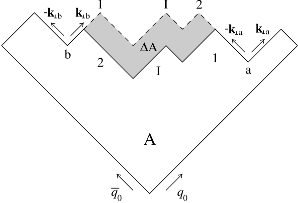
Figure 1: The decay of a Lund Model string spanning the space–time area $A$. The particles $1$ and $2$ are identical bosons and the particle(s) produced in between them is denoted by $I$. The two possible ways, $(\ldots,1,I,2,\ldots)$ and $(\ldots,2,I,1,\ldots)$, to produce the state are shown and the area difference between the two cases, $\Delta A$, is shaded. The two neighbouring vertices of the state with the two identical bosons are denoted by $a$ and $b$, and the transverse momenta of the quarks produced in the neighbouring vertices are $\pm{\bf k}_{\perp a}$ and $\pm{\bf k}_{\perp b}$, respectively.

In case there are two or more identical bosons the matrix element should be symmetrised and in general we obtain the symmetrised production amplitude

$${\cal M}=\sum_{{\cal P}}{\cal M}_{{\cal P}}$$ (5)

where the sum goes over all possible permutations of the identical particles. The squared amplitude occurring in Eq (3) will then be

$$|{\cal M}|^{2}=\sum_{{\cal P}}|{\cal M}_{{\cal P}}|^{2}\left(1+\sum_{{\cal P}^{\prime}\neq{\cal P}}\frac{2\mbox{Re}({\cal M}_{{\cal P}}{\cal M}_{{\cal P}^{\prime}}^{\ast})}{|{\cal M}_{{\cal P}}|^{2}+|{\cal M}_{{\cal P}^{\prime}}|^{2}}\right)$$ (6)

JETSET will provide the outer sum in Eq (6) by the generation of many events but it is evident that the model predicts a quantum mechanical interference weight, $w_{{\cal P}}$, for each given final state characterised by the permutation ${\cal P}$:

$$w_{{\cal P}}=1+\sum_{{\cal P}^{\prime}\neq{\cal P}}\frac{2\mbox{Re}({\cal M}_{{\cal P}}{\cal M}_{{\cal P}^{\prime}}^{\ast})}{|{\cal M}_{{\cal P}}|^{2}+{\cal M}_{{\cal P}^{\prime}}|^{2}}$$ (7)

In the Lund Model we note in particular for the case exhibited in Fig 1, with two identical bosons denoted 1 and 2 having a state $I$ in between, that the decay area is different if the two identical particles are exchanged. It is evident that the interference between the two permutation matrices will contain the area difference, $\Delta A$, and the resulting general weight formula will be

$$w_{{\cal P}}=1+\sum_{{\cal P}^{\prime}\neq{\cal P}}\frac{\textstyle\cos\frac{\textstyle\Delta A}{\textstyle 2\kappa}}{\textstyle\cosh\left(\frac{\textstyle b\Delta A}{\textstyle 2}+\frac{\textstyle\Delta(\sum{\bf k}^{2}_{\perp j})}{\textstyle 2\kappa}\right)}$$ (8)

where $\Delta$ stands for the difference between the configurations described by the permutations ${\cal P}$ and ${\cal P}^{\prime}$ and the sum is taken over all the vertices. In our MC implementation of the weight we replace the string constant $\kappa$ in the transverse momentum generation with the default (in JETSET) transverse width, $2\sigma^{2}$ (which is of the order of $\kappa$). The calculation of the weight function for $n$ identical bosons contains $n!-1$ terms and it is therefore from a computational point of view of exponential-type. We have in [3] introduced approximate methods reducing it to power-type instead and we refer for details to this work.

We have seen that the transverse and longitudinal components of the particles momenta stem from different generation mechanisms. This is clearly manifested in the weight in Eq (8) where they give different contributions. In the following we will therefore in some detail analyse the impact of this difference on the transverse and longitudinal correlation lengths, as implemented in the model.

In order to understand the properties of the weight in Eq (8) we again consider the simple case in Fig 1. The area difference of the two configurations depends upon the energy momentum vectors $p_{1},p_{2}$ and $p_{I}$ and can in a dimensionless and useful way be written as

$$\frac{\Delta A}{2\kappa}=\delta p\delta x_{L}$$ (9)

where $\delta p=p_{2}-p_{1}$ and $\delta x_{L}=(\delta t;0,0,\delta z)$ is a reasonable estimate of the space-time difference, along the surface area, between the production points of the two identical bosons.

In order to preserve the transverse momenta of the particles in the state $(1,I,2)$ it is necessary to change the generated ${\bf k}_{\perp}$ at the two internal vertices around the state $I$ during the permutation, i.e. to change the Gaussian weights. Also in this case we may write a formula similar to Eq (9) for the transverse momentum change:

$$\frac{\Delta(\sum{\bf k}_{\perp j}^{2})}{2\kappa}=\delta{\bf p}_{\perp}\delta{\bf x}_{\perp}$$ (10)

where ${\delta{\bf p}}_{\perp}$ is the difference ${\bf p}_{\perp 2}-{\bf p}_{\perp 1}$ and $\delta{\bf x}_{\perp}=({\bf k}_{\perp b}-(-{\bf k}_{\perp a}))/\kappa$. The two neighbouring vertices of the state $(1,I,2)$ ($(2,I,1)$) are denoted by $a$ and $b$ and ${\bf k}_{\perp b}+{\bf k}_{\perp a}$ corresponds to the states transverse momentum exchange to the outside. Therefore $\delta{\bf x}_{\perp}$ constitutes a possible estimate of the transverse distance between the production points of the pair.

For the general case when the permutation ${\cal P}^{\prime}$ is more than a two-particle exchange there are formulas similar to Eqs (9) and (10) although they are more complex (and the expressions do not vanish when only two of the exchanged particles have the same energy momentum).

It is evident from the considerations leading to Eqs (9) and (10) that only particles with a finite longitudinal distance and small relative energy momenta will give significant contributions to the weights. We also note that we are in this way describing longitudinal correlation lengths along the colour fields, inside which a given flavour combination is compensated. The corresponding transverse correlation length describes the tunneling (and in this model it provides a damping chaoticity).

The weight distribution we obtain is discussed in [3] (and with varying kaon and baryon content also below). It is strongly centered around unity although there are noticeable tails to both larger and smaller (even negative) weights. The total production probability is, however, positive and we find negligible changes in the JETSET default observables (besides the correlation functions) by this extension of the Lund model.

3 Results

Two-dimensional Bose-Einstein correlations in $e^{+}e^{-}$ annihilation have been analysed at lower energies than LEP by the TASSO collaboration [4]. Although they find that their data is compatible with a spherically symmetric correlation function they conclude that at least one order of magnitude of more data is required to obtain more detailed information. With the large statistics available from LEP we have therefore generated $q\bar{q}$-events at the $Z^{0}$ pole to investigate the properties of our model. Short-lived resonances like the $\rho$ and $K^{*}$ are allowed to decay before the BE-symmetrisation, while more long-lived ones are not affected.

We have analysed two-particle correlations in the Longitudinal Centre-of-Mass System (LCMS). For each pair of particles the LCMS is the system in which the sum of the two particles momentum components along the jet axis is zero, which of course also means that the sum of their momenta is perpendicular to the jet axis. The transverse and longitudinal momentum differences are then defined in the LCMS as

$$q_{t}=\sqrt{(p_{x2}-p_{x1})^{2}+(p_{y2}-p_{y1})^{2}}$$ (11)

$$q_{L}=|p_{z2}-p_{z2}|$$

where the jet axis is along the z-axis.

We have taken the ratio of the two-particle probability density of pions, $\rho_{2}$, with and without BE weights applied as the two-particle correlation function, $R_{2}$

$$R_{2}(p_{1},p_{2})=\frac{\rho_{2w}(p_{1},p_{2})}{\rho_{2}(p_{1},p_{2})}$$ (12)

and the resulting function is shown in Fig 2. It is clearly seen that it is not symmetric in $q_{L}$ and $q_{\perp}$ and in particular that the correlation length, as measured by the inverse of the width of the correlation function, is longer in the longitudinal than in the transverse direction. This difference remains for reasonable changes of the width in the transverse momentum generation. For comparison we have also analysed events where the Bose-Einstein effect has been simulated by the LUBOEI algorithm implemented in JETSET [5]. In LUBOEI the BE effect is simulated as a mean-field potential between identical bosons which is spherically symmetric in $Q$. Analysing only the initial particles and particles stemming from short-lived decays results for the LUBOEI events in a correlation function with identical transverse and longitudinal correlation lengths. The correlation lengths are in agreement with the source radii input to LUBOEI. Using all the final pion pairs, after all decays, in the analysis results in a small decrease in the transverse correlation length and of course a large decrease in the height for $q_{L}\simeq q_{\perp}\simeq 0$, while the longitudinal correlation length is rather unaffected. The pions from long lived decays affect the correlation lengths in the same way both for our model and for LUBOEI.

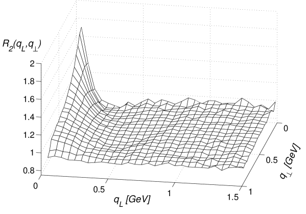
Figure 2: The ratio $R_{2}(q_{L},q_{\perp})$ of the number of charged pion pairs having relative four-momentum components $q_{L}$ and $q_{\perp}$ with and without Bose-Einstein weights applied. The sample consists of particles which are either initially produced or stemming from short-lived resonances.

In [3] it is shown that our model gives rise to genuine three-particle correlations. We will in this letter continue to investigate three-particle correlations and we will in particular use our knowledge of the different contributions to the weight function to study the genuine higher order correlations. We will also exhibit how the genuine higher order terms in the weight function mainly clusters particles in the longitudinal direction.

The total three-particle correlation function is in analogy with Eq (12)

$$R_{3}^{{}^{\prime\prime}}(p_{1},p_{2},p_{3})=\frac{\rho_{3w}(p_{1},p_{2},p_{3})}{\rho_{3}(p_{1},p_{2},p_{3})}$$ (13)

To get the genuine three-particle correlation function, $R_{3}$, the consequences of having two-particle correlations in the model have to be subtracted from $R_{3}^{{}^{\prime\prime}}$. To this aim we have calculated the weight taking into account only configurations where pairs are exchanged, $w^{{}^{\prime}}$. In this way the three-particle correlations which only are a consequence of lower order correlations can be defined as

$$R_{3}^{{}^{\prime}}(p_{1},p_{2},p_{3})=\frac{\rho_{3w^{{}^{\prime}}}(p_{1},p_{2},p_{3})}{\rho_{3}(p_{1},p_{2},p_{3})}$$ (14)

The genuine three-particle correlation function, $R_{3}$, is then given by

$$R_{3}=R_{3}^{{}^{\prime\prime}}-R_{3}^{{}^{\prime}}+1$$ (15)

Figure 3: $R_{3}^{{}^{\prime\prime}}(Q)$ and $R_{3}^{{}^{\prime}}(Q)$ are shown in the left figure, while the figure to the right shows $R_{3}(Q)$. The existence of genuine three-particle correlations is apparent.

We have analysed $R_{3}$ in one dimension as a function of the kinematical variable

$$Q=\sqrt{Q_{12}^{2}+Q_{13}^{2}+Q_{23}^{2}}~{}~{}~{}~{}\mbox{with}~{}~{}~{}~{}Q_{ij}^{2}=-(p_{i}-p_{j})^{2}$$ (16)

and in two dimensions we have used the following variables calculated in the LCMS for each triplet of identical bosons

$$q_{L}=\sqrt{q_{L12}^{2}+q_{L13}^{2}+q_{L23}^{2}}~{}~{}~{}~{}\mbox{with}~{}~{}~{}~{}q_{Lij}^{2}=(p_{zi}-p_{zj})^{2}$$ (17)

$$q_{\perp}=\sqrt{q_{\perp 12}^{2}+q_{\perp 13}^{2}+q_{\perp 23}^{2}}~{}~{}~{}~{}\mbox{with}~{}~{}~{}~{}q_{\perp ij}^{2}=({\bf p}_{\perp i}-{\bf p}_{\perp j})^{2}$$

where the $z$-axis is along the jet axis.

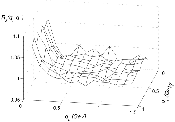
Figure 4: The ratio $R_{3}(q_{L},q_{\perp})$ of the number of triplets of charged pions with and without Bose-Einstein weights applied.

In Fig 3 the correlation functions $R_{3}^{{}^{\prime\prime}}(Q),R_{3}^{{}^{\prime}}(Q)$ and $R_{3}(Q)$ are shown, and the existence of genuine three-particle correlations in the model is clearly exhibited.

This way of getting the genuine correlations is not possible in an experimental situation, where one has to find other ways to get a $R_{3}^{{}^{\prime}}$ reference sample. We have suggested one possible option in [3] and the results in this letter are in agreement with the conclusions of that investigation. In the present analysis the contribution to the correlations from higher order configurations in the weight calculation is apparent. We note that $R_{3}$ flattens out earlier, i.e. for lower $Q$-values than $R_{3}^{{}^{\prime\prime}}$. This means that the genuine three-particle correlations have a longer correlation length compared to the consequences of lower order correlations. Performing the same analysis in two dimensions in the LCMS for each triplet results in the $R_{3}(q_{L},q_{\perp})$ distribution shown in Fig 4. The effect of the higher order terms is to pull the triplets closer in the longitudinal direction while the transverse direction is rather unaffected. This suggests that higher order correlations are more sensitive to the longitudinal stretching of the string field.

We have also studied the correlation length for pion pairs as a function of the final charged multiplicity and the kaon content of the state. Within statistical errors which are relatively large we see no dependence on either the charged multiplicity or the number of kaons. Since one might suspect that events with many pions are premiered by the re-weighting the average baryon and kaon content of the events have been investigated. We find that the changes of the average multiplicity of different kaon species as well as of the average multiplicity of protons and neutrons in the final state are much smaller than the experimental errors as summarised in [6].

References

- [1] M.G. Bowler, Z Phys. C29, 617 (1985)
- [2] B. Andersson and W. Hofmann, Phys. Lett. B169, 364 (1986)
- [3] B. Andersson and M. Ringnér, LU TP 97-07 and hep-ph/9704383 (1997)
- [4] M. Althoff et al. (TASSO Coll.), Z. Phys. C30, 355 (1986)
- [5] L. Lönnblad and T. Sjöstrand, Phys. Lett. B351, 293 (1995)
- [6] Particle Data Group, Phys. Rev. D54, 187 (1996)