Neutrino oscillations in a model with a source and detector

Abstract

We study the oscillations of neutrinos in a model in which the neutrino is coupled to a localized, idealized source and detector. By varying the spatial and temporal resolution of the source and detector we are able to model the full range of source and detector types ranging from coherent to incoherent. We find that this approach is useful in understanding the interface between the Quantum Mechanical nature of neutrino oscillations on the one hand and the production and detection systems on the other hand. This method can easily be extended to study the oscillations of other particles such as the neutral $K$ and $B$ mesons. We find that this approach gives a reliable way to treat the various ambiguities which arise when one examines the oscillations from a wave packet point of view. We demonstrate that the conventional oscillation formula is correct in the relativistic limit and that several recent claims of an extra factor of 2 in the oscillation length are incorrect. We also demonstrate explicitly that the oscillations of neutrinos which have separated spatially may be “revived” by a long coherent measurement.

I Introduction

The flavour oscillations of particles are a fascinating demonstration of quantum mechanics in the macroscopic world. Flavour oscillations can generically occur when the states which are produced and detected in a given experiment are superpositions of two or more eigenstates which have different masses. The oscillations of $K$ and $B$ mesons have been observed experimentally [1] and have been used to place stringent constraints on physics beyond the Standard Model. If neutrinos are massive, they too may oscillate, and this could lead to the resolution of the well-known solar neutrino problem [2, 3, 4]. More recently, the discussion of particle oscillations has been extended to include supersymmetric particles in supersymmetric extensions of the Standard Model [5].

The phenomenon of particle oscillations has been studied extensively and is generally thought to be very well understood. There nevertheless remain several subtle issues which continue to cause some confusion. The key to a complete understanding of any such issue lays in treating correctly the necessary interplay between the “classical” and “quantum” natures of the particles which are interfering to produce the oscillations. Thus, for example, the interference effect itself is purely “quantum” in nature (it requires that the particles be described by waves), and yet the resulting oscillations in space are only observable if the particles are sufficiently localized in space [6]. This example highlights the fact that any discussion of particle oscillations implicitly assumes that the mass eigenstates which are interfering to produce the oscillations are described by some sort of wave packets.

Despite the success of the wave packet approach in clarifying many aspects of the phenomenon of particle oscillations [6, 7, 8, 9], the approach is not without its own difficulties. The results of a given calculation will depend, for example, on the details of the initial mass eigenstate wave packets (including their shape, spectrum and relative normalization). One particularly difficult problem which arises is the conversion of the final time-evolved wave packets into an experimentally observable quantity: since it is generally the flux of particles which is measured in an experiment, one is required to calculate a current density rather than a probability density. The difference between a current density and a probability density, at least naively, involves a factor of the velocity $v$, which is very significant if the mass eigenstates have quite different masses. Thus, if one would calculate the probability density at the detector and integrate it over time, the resulting expression would have factors of $1/v$ pre-multiplying the various terms, leading to an enhancement of the terms corresponding to heavier mass eigenstates. In the case of neutrinos, as was noted in [8, 9, 10], this would skew the usual oscillation formula quite dramatically if one of the mass eigenstate neutrinos was non-relativistic. Efforts to construct an appropriate current density which retains the necessary wave packet features have had mixed success. A calculation in the kaon case appears to give reliable results [11], but it can be shown that unphysical effects arise if one attempts to define a suitable current when the mass eigenstates have very different masses [12].

There is another very striking apparent “ambiguity” which arises if one does not treat the delicate interplay between the classical and quantum natures of the particles correctly. In this case the “ambiguity” leads to an alleged error by a factor of “2” in the calculation of the oscillation length [13]. In order to understand the source of the ambiguity, we follow the discussion given by Lipkin [14]. Suppose we consider the oscillations in time of a system for which the initial and final states are not eigenstates of the free Hamiltonian. The phase of the interference term will then be given by $\phi(t)$$=$$(E_{1}-E_{2})t$, where $E_{i}$$\equiv$$(p^{2}+m_{i}^{2})^{1/2}$. Detectors do not measure oscillations directly as a function of time, however, so one needs somehow to convert this expression into an oscillation in terms of space. We may then, as is conventionally done, set $x$$=$$vt$, with $v$$=$$2p/(E_{1}+E_{2})$ representing a sort of average velocity. We then obtain the following phase in terms of $x$,

$$\phi_{\rm conv}(x)=\frac{(m_{1}^{2}-m_{2}^{2})x}{2p}.$$ (1)

This is the conventional (and correct) result for the phase difference. Let us now attempt to incorporate a classical aspect of the problem and argue that since the two mass eigenstates travel at different speeds, they will arrive at the detector at different times $t_{1}$ and $t_{2}$, related by $x$$=$$pt_{1}/E_{1}$$=$$pt_{2}/E_{2}$. Taking the phase of the interference term to be $\phi(t_{1},t_{2})$$=$$E_{1}t_{1}-E_{2}t_{2}$, we then obtain

$$\phi_{\rm new}(x)=\frac{(m_{1}^{2}-m_{2}^{2})x}{p},$$ (2)

which differs from the conventional phase difference, Eq. (1), by a factor of two. This result, were it correct, would indeed be rather remarkable.

The first resolution of this ambiguity was given by Lipkin [14] (see also Ref. [15]) who argued, on physical grounds, that the energies (rather than the momenta) of the two mass eigenstates should be set equal. In this case the oscillations are described in terms of distances directly (since it is the momenta of the two eigenstates which differ) and the “correct” oscillation formula is obtained. Lowe et al [16] and Kayser [17] have extended this discussion and have argued that the key to avoiding ambiguities is to ensure that one evaluates the wave functions of the mass eigenstates at precisely the same space-time point. That is, even though classically the mass eigenstates will arrive at the detector at different times, quantum mechanically the wave functions corresponding to different space-time points cannot interfere. Indeed the analysis leading to the expression in Eq. (2) involves interfering the wave functions for the two mass eigenstates at the same position but different times and hence gives the incorrect result. This issue is, in fact, quite subtle. For example a long coherent measurement in time may be used to “revive” particle oscillations even after the mass eigenstate wave packets have completely separated spatially [18]. Thus, wave packets arriving at the “classically” separated times $t_{1}$ and $t_{2}$ – and having negligible overlap in their wave packets – may still interfere to give rise to oscillations. There is then some sense in which wave functions corresponding to different space-time points may interfere.

In light of the issues presented above, it is our view that a proper treatment of the Quantum – Classical interface of particle oscillations should incorportate the source and the detector as key components of the system. In this paper we present a simple model for a particle source-detector system which addresses many of the above issues in a very natural and self-consistent way. We shall, for concreteness, consider the case of neutrino oscillations, but our approach could easily be adapted to other situations. The source and detector will be modeled by simple harmonic oscillators which are de-excited or excited by emitting or absorbing neutrinos of a given flavour. (Two-level “fermionic” source – detector systems could also be considered.) Having defined the model, it will be straightforward to calculate the oscillation probability as a function of the distance between the source and detector. The resulting expressions will be found to exhibit all of the known “wave packet” characteristics in the relativistic limit, but will also give useful insight into cases in which one or more of the mass eigenstates is non-relativistic. In particular, we will find no evidence for the enhancement of non-relativistic neutrinos which can occur in conventional wave packet analyses. Including the source explicitly in the calculation gives the added benefit that the characteristics of the initial wave packets corresponding to the various mass eigenstates are completely determined by the characteristics of the source and need not be put in by hand. Our approach is similar in spirit to the calculations in Refs. [19, 20], but is more transparent due to the simplified model which we consider. (See also Ref. [21] for a similar calculation performed within the context of elementary quantum mechanics.) One advantage of our simplified approach is that the dependence on the time-resolution of the detector is very clear. This will allow us to verify explicitly that a long coherent measurement in time may be used to revive the oscillations of particles whose wave packets have separated spatially. We shall also settle the issue of the “factor of 2” (hopefully) once and for all.

We begin in the next section by analyzing a simple model in which the neutrino is described by a complex scalar field. This field is coupled to two localized simple harmonic oscillators, representing the source and detector. Modeling the neutrino by a complex scalar field allows for a simpler and more complete evaluation of physical quantities than if a spinor field is used. In Sec. II A we study the case of a single neutrino species coupled to the source and detector. This allows for a careful analysis of the efficiency of our system at producing and detecting neutrinos of different masses. Although no oscillations are possible in this case, this calculation will be essential in interpreting the results when neutrino oscillations are present. In Sec. II B we couple several neutrino fields to the source and detector. This gives rise in a natural way to oscillations (as a function of the distance between the source and detector) in the probability for the source to decay and the detector to be excited. These are of course “neutrino oscillations.” Sec. II C contains a brief analysis of the non-relativistic case. We then extend our analysis in Sec. III to a more realistic model in which the neutrinos are described by Dirac spinor fields. These results are compared to the ones with a complex scalar field. We conclude in Sec. IV with a summary and discussion of our results.

II A Model for a Neutrino Source and Detector

The idea of using an idealized detector to clarify physically measurable quantities in Quantum Field Theory has been used extensively in the analysis of Quantum Fields in non-inertial frames and in gravitational backgrounds [23]. In our idealized model, we have chosen to couple the neutrino field to two harmonic oscillators, one representing a neutrino “source,” and the other representing a neutrino “detector.” The neutrinos are first taken to be complex scalar fields which simplifies the calculations considerably.

The physical picture which we have in mind is the following: we imagine our “source” and “detector” to be microscopic on the scale of some macroscopic “bulk” source and detector, but to also be very massive compared to the energy of the exchanged neutrino (so that the dynamical degrees of freedom of the source and detector may be ignored). Thus, for example, the source (detector) could represent some nucleus inside a bulk sample which undergoes beta decay (inverse beta decay). The spatial “widths” of the source and detector in our calculation are then widths appropriate to, say, nuclear or atomic dimensions. In principle, the oscillation probability which we calculate here should subsequently be averaged incoherently over the physical dimensions of the macroscopic source and detector, although we do not perform this average. If the size of the macroscopic source and detector are much smaller than the neutrino oscillation length (which they need to be in order to observe oscillations), then this averaging would have only a small effect.

The interactions at the source and detector will be made explicitly time dependent so that they may be turned “on” and “off.” This is in keeping with our physical picture. In general a real (microscopic) source or detector will be in an environment which is “noisy,” so that the coherent emission or absorption of a neutrino gets cut off after some time due to the interactions of the source or detector with its surrounding environment [9, 18]. The amount of time which the model source or detector spend being “on” is then related to the “coherence time” of the physical source or detector.

Our calculation proceeds as follows. We first write a Lagrangian which couples the source and detector to the neutrino field. In the initial state of the system, the source is in its first excited state (ready to emit a neutrino) and the detector is in its ground state. We then calculate the probability that at some time far in the future the source is found to be in its ground state and the detector in its first excited state. The model will be constructed in such a way that this interaction will correspond to exactly one neutrino being exchanged between the source and detector (to first non-vanishing order in perturbation theory.) In this approach, then, the neutrinos themselves are not observed, but are simply the exchange particles in the source-detector interaction.

A A Single Species of Neutrino

To describe our model, we begin with a single complex scalar field $\phi(x)$ and two oscillators $q_{1}(t)$ and $q_{2}(t)$ describing the source and detector, respectively. The action for our model is given by

$$S=\int d^{4}x\left({\cal L}_{\phi}^{0}+{\cal L}_{\rm int}\right)+\int dtL_{q}^{0},$$ (3)

where

$${\cal L}_{\phi}^{0} = -\phi^{\dagger}(x)\left(\Box+m^{2}\right)\phi(x),$$ (4)

$$L_{q}^{0} = \dot{q}_{1}^{\dagger}(t)\dot{q}_{1}(t)-\Omega_{1}^{2}q_{1}^{\dagger}(t)q_{1}(t)+\dot{q}_{2}^{\dagger}(t)\dot{q}_{2}(t)-\Omega_{2}^{2}q_{2}^{\dagger}(t)q_{2}(t),$$ (5)

$${\cal L}_{\rm int} = -\epsilon_{1}(t)\left(\phi^{\dagger}(x)q_{1}(t)h_{1}({\bf x})+\phi(x)q_{1}^{\dagger}(t)h_{1}^{*}({\bf x})\right)$$ (7)

$$-\epsilon_{2}(t)\left(\phi^{\dagger}(x)q_{2}(t)h_{2}({\bf x})+\phi(x)q_{2}^{\dagger}(t)h_{2}^{*}({\bf x})\right).$$

The functions $\epsilon_{i}(t)$ are explicit functions of time which allow us to “turn on” and “turn off” the interactions, and the functions $h_{1}({\bf x})$ ($h_{2}({\bf x})$) are smooth functions of ${\bf x}$ which vanish outside the source (detector).

We quantize the free fields in the usual way, requiring

$$\left[\phi({\bf x},t),\pi({\bf y},t)\right] = i\delta^{3}({\bf x}-{\bf y}),$$ (8)

$$\left[q_{i}(t),p_{i}(t)\right] = i.$$ (9)

All other commutators are taken to vanish. The field operators may then be expressed in terms of creation and annihilation operators as follows

$$\phi(x) = \int d\tilde{k}\left(a(k)e^{-ik\cdot x}+b^{\dagger}(k)e^{ik\cdot x}\right),$$ (10)

$$q_{i}(t) = \frac{1}{2\Omega_{i}}\left(A_{i}e^{-i\Omega_{i}t}+B_{i}^{\dagger}e^{i\Omega_{i}t}\right),$$ (11)

where

$$d\tilde{k}\equiv\frac{d^{3}k}{(2\pi)^{3}2E}$$ (12)

and where the annihilation and creation operators satisfy the commutation relations

$$\left[a(k),a^{\dagger}(k^{\prime})\right] = \left[b(k),b^{\dagger}(k^{\prime})\right]=(2\pi)^{3}2E\delta^{3}({\bf k}-{\bf k}^{\prime}),$$ (13)

$$\left[A_{i},A_{i}^{\dagger}\right] = \left[B_{i},B_{i}^{\dagger}\right]=2\Omega_{i}.$$ (14)

We interpret $a^{\dagger}(k)$ and $a(k)$ in the usual way as the operators which create and annihilate, respectively, a neutrino state with four-momentum $k$. $b^{\dagger}(k)$ and $b(k)$ act similarly with respect to the anti-neutrino states. The operators $A_{i}^{\dagger}$ and $A_{i}$ and $B_{i}^{\dagger}$ and $B_{i}$ interpolate between the energy levels of the harmonic oscillators.

We take as our initial state

$$|s,-\infty\rangle=|0;1;0\rangle\equiv|0\rangle_{\phi}\otimes|1\rangle_{1}\otimes|0\rangle_{2}$$ (15)

in which

$$|1\rangle_{i}\equiv A_{i}^{\dagger}|0\rangle_{i}$$ (16)

represents the first excited state of the oscillator $i$ and in which $|0\rangle_{\phi}$ is the neutrino vacuum state. We wish to calculate the amplitude for the process in which the source de-excites to its ground state and the detector is excited to its first excited state. That is,

$${\cal A}\equiv\langle 0;0;1|s,\infty\rangle=\langle 0;0;1|T{\rm exp}\left[-i\int_{-\infty}^{\infty}H^{S}(t^{\prime})dt^{\prime}\right]|s,-\infty\rangle,$$ (17)

in which $H^{S}$ represents the Hamiltonian in the Schrödinger picture. The modulus squared of this amplitude is the probability for the transition to take place.

We shall assume the couplings in the interaction Hamiltonian to be sufficiently small that the amplitude in Eq. (17) is always much less than unity. This is of course always the case in the real-world situation which we are attempting to model – neutrino interactions are so weak that perturbation theory is always valid. It is then straightforward to evaluate (17) using standard techniques to obtain to leading order and up to an over-all unobservable phase,

$${\cal A}=-\frac{1}{2}\langle 0;0;1|T\left[\int_{-\infty}^{\infty}dt^{\prime}dt^{\prime\prime}H_{\rm int}^{H}(t^{\prime})H_{\rm int}^{H}(t^{\prime\prime})\right]|0;1;0\rangle,$$ (18)

where $H_{\rm int}^{H}(t)$ refers to the interaction Hamiltonian evaluated in terms of the free fields in the Heisenberg picture at time $t$. The above expression may be evaluated explicitly in terms of neutrino propagators [19, 20] for arbitrary turn-on/off functions $\epsilon_{i}(t)$. We find it simpler, however, to “design” the turn on/off functions so that the source and detector are never on at the same time, and, furthermore, so that the source always turns on first and only then the detector. (This avoids the unphysical situation in which the detector emits an anti-neutrino which is subsequently absorbed by the source. The amplitude for this process would in any case be very small since it violates energy conservation.) Under this assumption only one of the time-orderings in the propagator gets picked up and ${\cal A}$ may be evaluated using Eqs. (10), (11), (13), (14) and (16) to obtain

$${\cal A} = -\langle 0;0;1|\int dt^{\prime}dt^{\prime\prime}d^{3}x^{\prime}d^{3}x^{\prime\prime}\epsilon_{1}(t^{\prime})\epsilon_{2}(t^{\prime\prime})$$ (20)

$$\;\;\times\phi(x^{\prime\prime})q_{2}^{\dagger}(t^{\prime\prime})h_{2}^{*}({\bf x}^{\prime\prime})\phi^{\dagger}(x^{\prime})q_{1}(t^{\prime})h_{1}({\bf x}^{\prime})|0;1;0\rangle$$

$$= -\int dt^{\prime}dt^{\prime\prime}d^{3}x^{\prime}d^{3}x^{\prime\prime}d\tilde{k}\epsilon_{1}(t^{\prime})\epsilon_{2}(t^{\prime\prime})h_{1}({\bf x}^{\prime})h_{2}^{*}({\bf x}^{\prime\prime})$$ (22)

$$\;\;\times\exp\left[-i(E-\Omega_{2})t^{\prime\prime}+i(E-\Omega_{1})t^{\prime}+i{\bf k}\cdot({\bf x}^{\prime\prime}-{\bf x}^{\prime})\right].$$

Since the amplitude is proportional to $\langle 0|\phi(x^{\prime\prime})\phi^{\dagger}(x^{\prime})|0\rangle$, it is clear from Eq. (10) that this interaction corresponds to the creation and subsequent annihilation of a single neutrino.

In order to proceed further we choose $h_{1}$, $h_{2}$ and $\epsilon_{1}$ to be Gaussians since this allows many of the integrals to be evaluated exactly. Setting

$$h_{1}({\bf x}) = \left(\sqrt{2\pi}\sigma_{x_{1}}\right)^{-3}e^{-|{\bf x}|^{2}/{2\sigma_{x_{1}}^{2}}},$$ (23)

$$h_{2}({\bf x}) = \left(\sqrt{2\pi}\sigma_{x_{2}}\right)^{-3}e^{-|{\bf x}-{\bf x}_{D}|^{2}/{2\sigma_{x_{2}}^{2}}},$$ (24)

$$\epsilon_{1}(t) = \epsilon_{1}^{0}e^{-t^{2}/2\sigma_{t_{1}}^{2}}$$ (25)

we obtain

$${\cal A} = -\left(\frac{\sqrt{2\pi}\epsilon_{1}^{0}\sigma_{t_{1}}}{4\pi^{2}x_{D}}\right)\int_{-\infty}^{\infty}dt^{\prime\prime}\epsilon_{2}(t^{\prime\prime})\int_{m}^{\infty}dE\exp\left[-i(E-\Omega_{2})t^{\prime\prime}-\frac{1}{2}(E-\Omega_{1})^{2}\sigma_{t_{1}}^{2}\right.$$ (27)

$$\left.\;\;-\frac{1}{2}k^{2}(\sigma_{x_{1}}^{2}+\sigma_{x_{2}}^{2})\right]\sin(kx_{D}),$$

where

$$k\equiv\sqrt{E^{2}-m^{2}}.$$ (28)

Before choosing an explicit form for $\epsilon_{2}(t)$, which determines characteristics of the detector, let us make a few observations regarding the above expression for the amplitude. First of all, for large $x_{D}$, the amplitude decreases like $x_{D}^{-1}$ so that the probability falls like $x_{D}^{-2}$, as expected on geometrical grounds in three dimensions. At the origin, however, the amplitude does not diverge (despite the $1/x_{D}$ factor), due to the sine function in the integrand. A second observation is that conservation of energy at the source and of momentum at both the source and detector are governed by the relative sizes of $\sigma_{t_{1}}$, $\sigma_{x_{1}}$ and $\sigma_{x_{2}}$. This situation is in accordance with the uncertainty principle (and is in fact necessary, as discussed above, in order to observe oscillations). In general, neither energy nor momentum need be conserved exactly if the source and detector are localized in space and time. The specific set-up which we have chosen favours energies close to the energy of the excited source, $\Omega_{1}$, and momenta close to zero. This latter point is due to the fact that our souce and detector have no dynamical degrees of freedom – they cannot recoil when a neutrino is emitted or absorbed – and thus the neutrino gets all of its momentum from the uncertainties in the positions of the source and detector. In order to avoid the problem that low momenta are favoured, we shall typically choose to set $\sigma_{t_{1}}$$\gg$$\sigma_{x_{1,2}}$ in our numerical work below. When several neutrino fields are coupled to the source and detector, this will mean that the energies of the mass eigenstates will be approximately equal, while their momenta will be determined by their energies. Furthermore, the sizes of the neutrino wave packets will then be determined more by the amount of time for which the source emits an uninterrupted wave-train than by the localization of the source-field interaction in configuration space. In Sec. III, when we extend our analysis to fermionic neutrinos, we will allow the source to decay by emitting both a neutrino and its associated lepton. In this case the neutrino’s momentum will no longer be centered about $k$$\approx$$0$.

Let us now study the system as a function of the coherence time of the detector. At one extreme we can imagine that a given (microscopic) detector is turned on for the entire time that the neutrino “wave packet” passes by. This is an ultimately “coherent” detection event. Another possibility is that a given microscopic detector turns on and off without sampling the entire wave packet. In order to model the former scenario we use a simple step function for $\epsilon_{2}$, while for the latter case we use a gaussian:

$$\epsilon_{2}^{\rm step}(t) \equiv \epsilon_{2}^{0}\theta(t_{2}-t)\theta(t-t_{1}),$$ (29)

$$\epsilon_{2}^{\rm gauss}(t) \equiv \epsilon_{2}^{0}e^{-(t-t_{D})^{2}/2\sigma_{t_{2}}^{2}}.$$ (30)

The step function detector turns on abruptly at time $t_{1}$ and off again abruptly at time $t_{2}$ (with $t_{1}$ and $t_{2}$ chosen such that the entire wave packet passes by while the detector is on), while the gaussian detector turns on and off gradually at a time centered around $t_{D}$. Since the coherent (step function) detector “catches” the entire wave packet, there is no need to integrate the resulting expression for the probability over time. This is not the case for the incoherent (gaussian) detector: since each individual microscopic detector sees only a piece of the wave packet, one must sum incoherently over all of the microscopic detectors in order to correctly model the response of the bulk detector. If there are many microscopic detectors in the bulk detector, this incoherent sum corresponds to integrating the expression for the probability over $t_{D}$.

It is straightforward to evaluate the amplitudes for both types of detectors and we obtain

$${\cal A}_{\rm step} = \tilde{N}(t_{2}-t_{1})\int_{m}^{\infty}dE\,\frac{\sin\left[(E-\Omega_{2})(t_{2}-t_{1})/2\right]}{\left[(E-\Omega_{2})(t_{2}-t_{1})/2\right]}\,\exp\left[-\frac{i}{2}(E-\Omega_{2})(t_{1}+t_{2})\right.$$ (32)

$$\left.\;\;-\frac{1}{2}(E-\Omega_{1})^{2}\sigma_{t_{1}}^{2}-\frac{1}{2}k^{2}(\sigma_{x_{1}}^{2}+\sigma_{x_{2}}^{2})\right]\sin(kx_{D}),$$

$${\cal A}_{\rm gauss} = \tilde{N}\sqrt{2\pi}\sigma_{t_{2}}\int_{m}^{\infty}dE\exp\left[-\frac{1}{2}(E-\Omega_{1})^{2}\sigma_{t_{1}}^{2}-\frac{1}{2}(E-\Omega_{2})^{2}\sigma_{t_{2}}^{2}\right.$$ (34)

$$\left.\;\;-\frac{1}{2}k^{2}(\sigma_{x_{1}}^{2}+\sigma_{x_{2}}^{2})-i(E-\Omega_{2})t_{D}\right]\sin(kx_{D}),$$

where

$$\tilde{N}\equiv-\frac{\epsilon_{1}^{0}\epsilon_{2}^{0}\sigma_{t_{1}}}{(2\pi)^{3/2}x_{D}}.$$ (35)

It is not possible in general to obtain analytic closed-form solutions of these integrals, but they are simple to evaluate numerically. In so doing, we obtain exact (to second order in perturbation theory) solutions to the problem which we are studying, including all effects due to the spreading of the neutrino wave packets. Alternatively, we may, in some cases, find reliable approximations for these integrals. Such is the case for the step function detector if the neutrino’s mass is not too close to the production and detection thresholds ($m$$\ll$$\Omega_{i}-1/\sigma_{t_{1}}$). Taking $t_{1}$ to be a time before the first bit of neutrino flux arrives at the detector and $t_{2}$ to be a time after the entire neutrino wave packet has passed (formally, $t_{2}$$\to$$\infty$), we find

$$\lim_{t_{2}\rightarrow\infty}{\cal A}_{\rm step}(x_{D},t_{1},t_{2}) \simeq -i\tilde{N}\pi\exp\left[i\bar{k}x_{D}-\frac{1}{2}(\Omega_{2}-\Omega_{1})^{2}\sigma_{t_{1}}^{2}\right.$$ (37)

$$\left.\;\;\;\;-\frac{1}{2}(\Omega_{2}^{2}-m^{2})(\sigma_{x_{1}}^{2}+\sigma_{x_{2}}^{2})\right],$$

where $\bar{k}$$\equiv$$(\Omega_{2}^{2}-m^{2})^{1/2}$. (The details of this calculation may be found in Appendix A.) Note that the coherent detector “picks out” momenta corresponding to the energy $\Omega_{2}$.

The modified “probability” associated with the above amplitude is given by

$${\cal P}_{\rm step}(x_{D})\equiv\left|{\cal A}_{\rm step}(x_{D})\right|^{2}/\tilde{N}^{2},$$ (38)

where we have dropped the implicit dependence on $t_{1}$ and $t_{2}$. We have also divided through by $\tilde{N}^{2}$ because the value of that constant (including the fall-off as $x_{D}^{-2}$) is not really of interest to us since in any calculation of the oscillation probability $\tilde{N}^{2}$ always factors out. Taking the ratio of this probability for two different values of the mass reveals that the system is more efficient at producing and detecting higher-mass neutrinos:

$$\frac{{\cal P}_{\rm step}(m;x_{D})}{{\cal P}_{\rm step}(m^{\prime};x_{D})}\simeq\exp\left[(m^{2}-m^{\prime 2})(\sigma_{x_{1}}^{2}+\sigma_{x_{2}}^{2})\right].$$ (39)

The mass-dependence of the source/detector system arises due to the fact that our source and detector favour neutrino states with momenta close to zero. This feature was predicted already in the discussion following Eq. (27) and is due to the fact that the source and detector in our model cannot “recoil” and thus the neutrino gets all of its momentum from the uncertainty in the positions of the source and detector. Thus the upper limit on the neutrino’s momentum is given by $k_{\rm max}$$\sim$$1/\sigma_{x_{1,2}}$. Note that this preference for non-relativistic neutrinos is essentially a quirk of our model and should not be viewed as a physical effect. The mass-dependence of the system can be minimized by setting $\sigma_{x_{1,2}}$ to be much less than $\Omega_{1,2}^{-1}$. In such cases, the step function detector becomes nearly “ideal;” that is, it detects neutrinos of different masses with nearly the same efficiency.

We now turn to the gaussian detector and define a modified probability in analogy with Eq. (38)

$${\cal P}_{\rm gauss}(x_{D},t_{D},\sigma_{t_{2}})\equiv\left|{\cal A}_{\rm gauss}(x_{D},t_{D},\sigma_{t_{2}})\right|^{2}/\tilde{N}^{2}.$$ (40)

This expression gives the probability that a given microscopic detector – turned on for a time $\sigma_{t_{2}}$ centered around the time $t_{D}$ – is excited. We need to convert this expression into one giving the probability that the bulk detector “detects” the neutrino (i.e., that one of the micropscopic detectors is excited.) We assume that the bulk detector is “on” for all $t_{D}$$>$$0$ – in the sense that at any given time many of the microscopic detectors are “on” – but that the microscopic detectors themselves turn on and off randomly, so that the number which are “on” at any given time is roughly constant. Then the probability that the bulk detector “detects” the neutrino is proportional to the integral of Eq. (40) over $t_{D}$. We thus refer to this type of bulk detector as an “incoherent” detector, since we sum the probability incoherently over different times.

The time integral of Eq. (40) may actually be done explicitly. Let us define the following (unnormalized) time-integrated probability

$${\cal P}_{\rm incoh}(x_{D},\sigma_{t_{2}})\equiv\int_{0}^{\infty}dt_{D}{\cal P}_{\rm gauss}(x_{D},t_{D},\sigma_{t_{2}}).$$ (42)

Since the integrand is symmetric under $t_{D}$$\rightarrow$$-t_{D}$, we may formally extend the integration to negative infinity and divide by two. The time integral then reduces to a delta function in energy and allows us to perform one of the energy integrals. As a result, we obtain

$${\cal P}_{\rm incoh}(x_{D},\sigma_{t_{2}}) = 2\pi^{2}\sigma_{t_{2}}^{2}\int_{m}^{\infty}dE\exp\left[-(E-\Omega_{1})^{2}\sigma_{t_{1}}^{2}-(E-\Omega_{2})^{2}\sigma_{t_{2}}^{2}\right.$$ (44)

$$\left.\;\;-k^{2}(\sigma_{x_{1}}^{2}+\sigma_{x_{2}}^{2})\right]\sin^{2}(kx_{D}).$$

If $m$$\ll$$\Omega_{i}-1/\sigma_{t_{i}}$ and $\sigma_{t_{1,2}}$$\gg$$\sigma_{x_{1,2}}$ (the latter condition is always assumed) then we may approximate the above expression by setting $\sin^{2}(kx_{D})$$\approx$$1/2$ to yield

$${\cal P}_{\rm incoh}(x_{D},\sigma_{t_{2}}) \simeq \frac{\pi^{5/2}\sigma_{t_{2}}^{2}}{\left(\sigma_{t_{1}}^{2}+\sigma_{t_{2}}^{2}+\sigma_{x_{1}}^{2}+\sigma_{x_{2}}^{2}\right)^{1/2}}\exp\left[m^{2}(\sigma_{x_{1}}^{2}+\sigma_{x_{2}}^{2})\right]$$ (46)

$$\;\;\times\exp\left[\frac{\left(\Omega_{1}\sigma_{t_{1}}^{2}+\Omega_{2}\sigma_{t_{2}}^{2}\right)^{2}}{\left(\sigma_{t_{1}}^{2}+\sigma_{t_{2}}^{2}+\sigma_{x_{1}}^{2}+\sigma_{x_{2}}^{2}\right)}-\Omega_{1}^{2}\sigma_{t_{1}}^{2}-\Omega_{2}^{2}\sigma_{t_{2}}^{2}\right].$$

Thus, under the above conditions the “incoherent” gaussian detector has the same mass-dependence as the step function detector does (c.f. Eq. (39)):

$$\frac{{\cal P}_{\rm incoh}(m;x_{D},\sigma_{t_{2}})}{{\cal P}_{\rm incoh}(m^{\prime};x_{D},\sigma_{t_{2}})}\simeq\exp\left[(m^{2}-m^{\prime 2})(\sigma_{x_{1}}^{2}+\sigma_{x_{2}}^{2})\right].$$ (47)

This fact is rather remarkable and shows again that it is correct to perform the time integral in Eq. (42).

Fig. 1 shows a plot of the time-integrated probability, Eq. (44), as a function of the neutrino mass for two different values of $\sigma_{x_{1,2}}$. This probability may be regarded as giving a measure of the efficiency with which the system produces and detects a neutrino of a given mass. For convenience, the probabilities have been normalized to their values at $m$$=$$0$. In each case, the solid line gives the exact result and the dashed line shows the approximation for non-threshold masses derived in Eq. (46). Clearly the approximation is quite good if the mass is not too close to the neutrino production and detection thresholds. Furthermore, it is clear that this detector can be made “ideal” (that is, the probability to detect a neutrino may be made mass-independent) by using suitably small values for $\sigma_{x_{1,2}}$. The mass-dependence for large $\sigma_{x_{1,2}}$ occurs for the same reason as in the case of the step function detector and is due to the fact that the source and detector in our model cannot recoil (see the discussion following Eq. (39)). The dash-dotted line shows a plot of $1/v(m)$ for comparison. This would be the analogous efficiency found in a wave packet calculation [8]. Since our detector may be made mass-independent by a suitable choice of the $\sigma_{x_{i}}$, we see that a “well designed” detector will not exhibit such an effect.

B Several Neutrinos

Now that we have studied the characteristics of the source/detector system in the single-neutrino case, we turn to the case in which there are several neutrino fields coupled to the source and detector. Suppose that there are $N$ different neutrino mass eigenstates. Then, in order to model the real-life situation, we suppose that there are also several different types of sources and detectors, each of which couple to a “weak eigenstate” which is a given unitary linear combination of the neutrino mass eigenstates. The action of Eq. (3) is then generalized to

$$S=\int d^{4}x\left({\cal L}_{\phi}^{0}+{\cal L}_{\rm int}\right)+\int dtL_{q}^{0},$$ (48)

where

$${\cal L}_{\phi}^{0} = -\sum_{i}\phi^{\dagger}_{i}(x)\left(\Box+m^{2}_{i}\right)\phi_{i}(x),$$ (49)

$$L_{q}^{0} = \sum_{\alpha}\left[\dot{q}_{1}^{\alpha\dagger}(t)\dot{q}_{1}^{\alpha}(t)-\Omega_{1}^{\alpha 2}q_{1}^{\alpha\dagger}(t)q_{1}^{\alpha}(t)+\dot{q}_{2}^{\alpha\dagger}(t)\dot{q}_{2}^{\alpha}(t)-\Omega_{2}^{\alpha 2}q_{2}^{\alpha\dagger}(t)q_{2}^{\alpha}(t)\right],$$ (50)

$${\cal L}_{\rm int} = -\sum_{\alpha,i}\left[\epsilon_{1}(t)\left({\cal U}_{\alpha i}^{*}\phi^{\dagger}_{i}(x)q_{1}^{\alpha}(t)h_{1}({\bf x})+{\cal U}_{\alpha i}\phi_{i}(x)q_{1}^{\alpha\dagger}(t)h_{1}^{*}({\bf x})\right)\right.$$ (52)

$$\left.\;\;\;\;\;\;+\epsilon_{2}(t)\left({\cal U}_{\alpha i}^{*}\phi^{\dagger}_{i}(x)q_{2}^{\alpha}(t)h_{2}({\bf x})+{\cal U}_{\alpha i}\phi_{i}(x)q_{2}^{\alpha\dagger}(t)h_{2}^{*}({\bf x})\right)\right],$$

and in which ${\cal U}$ is a unitary matrix. Note that the subscripts “1” and “2” on the functions $\epsilon$ and $h$ and on the fields $q$ refer, respectively, to the source and detector. These should not be confused with the subscripts on the fields $\phi$ which refer to the mass eigenstates. Also note that we have taken $\epsilon$ and $h$ to be independent of the flavour or mass eigenstate in question. In principle there could be such a dependence, but including it would unnecessarily complicate our analysis. In what follows, we shall also set $\Omega_{i}^{\alpha}$$=$$\Omega_{i}$, for all $\alpha$, in order to “idealize” our sources and detectors.

The experimental set-up which we wish to consider is a simple generalization of that given in the previous section. In this case we imagine that the initial state of the system has an $\alpha$-flavour “source” oscillator in its first excited state and that the final state has a $\beta$-flavour “detector” oscillator in its first excited state. The amplitude for this process may then be calculated as in the single-neutrino case and we find

$${\cal A}_{\alpha\rightarrow\beta} = -\sum_{i,j}{\cal U}_{\beta j}{\cal U}_{\alpha i}^{*}\langle 0;0;1_{\beta}|\int dt^{\prime}dt^{\prime\prime}d^{3}x^{\prime}d^{3}x^{\prime\prime}\epsilon_{1}(t^{\prime})\epsilon_{2}(t^{\prime\prime})$$ (54)

$$\;\;\times\phi_{j}(x^{\prime\prime})q_{2}^{\beta\dagger}(t^{\prime\prime})h_{2}^{*}({\bf x}^{\prime\prime})\phi^{\dagger}_{i}(x^{\prime})q_{1}^{\alpha}(t^{\prime})h_{1}({\bf x}^{\prime})|0;1_{\alpha};0\rangle$$

$$= -\sum_{i}{\cal U}_{\beta i}{\cal U}_{\alpha i}^{*}\int dt^{\prime}dt^{\prime\prime}d^{3}x^{\prime}d^{3}x^{\prime\prime}d\tilde{k}_{i}\epsilon_{1}(t^{\prime})\epsilon_{2}(t^{\prime\prime})h_{1}({\bf x}^{\prime})h_{2}^{*}({\bf x}^{\prime\prime})$$ (56)

$$\;\;\times\exp\left[-i(E_{i}-\Omega_{2})t^{\prime\prime}+i(E_{i}-\Omega_{1})t^{\prime}+i{\bf k}\cdot({\bf x}^{\prime\prime}-{\bf x}^{\prime})\right],$$

in which we have defined

$$E_{i} \equiv \sqrt{k^{2}+m_{i}^{2}}.$$ (57)

Taking $h_{1}$, $h_{2}$ and $\epsilon_{1}$ to be gaussians with widths $\sigma_{x_{1}}$, $\sigma_{x_{2}}$ and $\sigma_{t_{1}}$ as in the single-neutrino case (see Eqs. (23), (24) and (25)), we may further simplify this expression

$${\cal A}_{\alpha\rightarrow\beta} = -\left(\frac{\sqrt{2\pi}\epsilon_{1}^{0}\sigma_{t_{1}}}{4\pi^{2}x_{D}}\right)\sum_{i}{\cal U}_{\beta i}{\cal U}_{\alpha i}^{*}\int_{-\infty}^{\infty}dt^{\prime\prime}\epsilon_{2}(t^{\prime\prime})\int_{m_{i}}^{\infty}dE\exp\left[-i(E-\Omega_{2})t^{\prime\prime}\right.$$ (59)

$$\left.\;\;-\frac{1}{2}(E-\Omega_{1})^{2}\sigma_{t_{1}}^{2}-\frac{1}{2}k_{i}^{2}(\sigma_{x_{1}}^{2}+\sigma_{x_{2}}^{2})\right]\sin(k_{i}x_{D}),$$

where

$$k_{i}\equiv\sqrt{E^{2}-m_{i}^{2}}.$$ (60)

This expression is clearly just a simple generalization of Eq. (27). The final step in our calculation is to substitute the expressions (29) and (30) for $\epsilon_{2}(t)$ in the step function and gaussian detector cases. This yields

$${\cal A}^{\rm step}_{\alpha\rightarrow\beta} = \tilde{N}(t_{2}-t_{1})\sum_{i}{\cal U}_{\beta i}{\cal U}_{\alpha i}^{*}\int_{m_{i}}^{\infty}dE\,\frac{\sin\left[(E-\Omega_{2})(t_{2}-t_{1})/2\right]}{\left[(E-\Omega_{2})(t_{2}-t_{1})/2\right]}\,\sin(k_{i}x_{D})$$ (62)

$$\times\exp\left[-\frac{i}{2}(E-\Omega_{2})(t_{1}+t_{2})-\frac{1}{2}(E-\Omega_{1})^{2}\sigma_{t_{1}}^{2}-\frac{1}{2}k_{i}^{2}(\sigma_{x_{1}}^{2}+\sigma_{x_{2}}^{2})\right],$$

$${\cal A}^{\rm gauss}_{\alpha\rightarrow\beta} = \tilde{N}\sqrt{2\pi}\sigma_{t_{2}}\sum_{i}{\cal U}_{\beta i}{\cal U}_{\alpha i}^{*}\int_{m_{i}}^{\infty}dE\exp\left[-\frac{1}{2}(E-\Omega_{1})^{2}\sigma_{t_{1}}^{2}-\frac{1}{2}(E-\Omega_{2})^{2}\sigma_{t_{2}}^{2}\right.$$ (64)

$$\left.\;\;-\frac{1}{2}k_{i}^{2}(\sigma_{x_{1}}^{2}+\sigma_{x_{2}}^{2})-i(E-\Omega_{2})t_{D}\right]\sin(k_{i}x_{D}),$$

where $\tilde{N}$ is defined in (35).

We are finally in a position to define the oscillation probability as a function of distance for the two cases. In both cases our definition of the probability is a “physical” one. We imagine that the source produces neutrinos of type $\alpha$ ($\alpha$$=$$e,\mu,\tau,\ldots$) and that we set a $\beta$-neutrino detector at some distance $x_{D}$ from the source. We prepare the source (or an ensemble of identically prepared sources) in an excited state, wait a long period of time, and then check to see if the detector has been excited. After repeating this experiment enough times to get good statistics, we repeat the procedure with a $\beta^{\prime}$-neutrino detector, and so on. The probability to observe a $\beta$ neutrino is then simply the number of events observed in “$\beta$-mode” divided by the total number of events in all modes. Since we have attempted to make our source/detector system as “ideal” as possible, there are no further corrections for detector efficiencies or other effects of that nature. The normalized coherent and incoherent oscillation probabilities may then be defined as

$${\cal P}_{\alpha\rightarrow\beta}^{\rm coh}(x_{D}) = \lim_{t_{2}\rightarrow\infty}\frac{\left|{\cal A}^{\rm step}_{\alpha\rightarrow\beta}(x_{D},t_{1},t_{2})\right|^{2}}{\sum_{\beta^{\prime}}\left|{\cal A}^{\rm step}_{\alpha\rightarrow\beta^{\prime}}(x_{D},t_{1},t_{2})\right|^{2}},$$ (65)

$${\cal P}_{\alpha\rightarrow\beta}^{\rm incoh}(x_{D},\sigma_{t_{2}}) = \frac{\int_{0}^{\infty}dt_{D}\left|{\cal A}^{\rm gauss}_{\alpha\rightarrow\beta}(x_{D},t_{D},\sigma_{t_{2}})\right|^{2}}{\sum_{\beta^{\prime}}\int_{0}^{\infty}dt_{D}\left|{\cal A}^{\rm gauss}_{\alpha\rightarrow\beta^{\prime}}(x_{D},t_{D},\sigma_{t_{2}})\right|^{2}}.$$ (66)

It is understood in the first expression that $t_{1}$ is taken to be some time before the first bit of neutrino “flux” arrives at the detector.

The expressions which we have derived for our two types of detectors are in forms which are amenable to numerical calculation. The coherent probability may be found after a single integration over energy and the incoherent probability requires two integrations, one over energy and one over time. In the two-neutrino case, the time integral in Eq. (66) may be done by hand, but this is not possible in general for more neutrinos. The reason for this is that the integrand is no longer symmetric under $t_{D}$$\rightarrow$$-t_{D}$ due to the possible presence of phases in the mixing matrix ${\cal U}$.

Let us examine the case with two flavours in some detail. In this case, the matrix ${\cal U}$ may be taken to be a real orthogonal matrix parametrized by one angle, $\theta$. The time integral in the numerator of (66) may be performed explicitly and we find

$$\int_{0}^{\infty}dt_{D}\left|{\cal A}^{\rm gauss}_{\alpha\rightarrow\beta}(x_{D},t_{D},\sigma_{t_{2}})\right|^{2} =$$ (69)

$$2\pi^{2}\sigma_{t_{2}}^{2}\tilde{N}^{2}\sum_{i,j}{\cal U}_{\beta i}{\cal U}_{\beta j}{\cal U}_{\alpha i}{\cal U}_{\alpha j}\int_{{\rm max}(m_{i},m_{j})}^{\infty}dE\sin(k_{i}x_{D})\sin(k_{j}x_{D})$$

$$\times\exp\left[-(E-\Omega_{1})^{2}\sigma_{t_{1}}^{2}-(E-\Omega_{2})^{2}\sigma_{t_{2}}^{2}-(E^{2}-(m_{i}^{2}+m_{j}^{2})/2)(\sigma_{x_{1}}^{2}+\sigma_{x_{2}}^{2})\right].$$

Fig. 2 shows several plots of the flavour-conserving probability ${\cal P}_{e\rightarrow e}(x_{D})$ as a function of $x_{D}$ for two relativistic neutrinos, using both the “coherent” and the “incoherent” detector. The various parameters chosen for the plot are as indicated in the figure. Recall that $\Omega_{1}$ and $\Omega_{2}$ (set equal here) are the energies of the excited source and detector, respectively. Since we have chosen to set $\sigma_{x_{i}}$$\ll$$\sigma_{t_{i}}$, the energies of the mass eigenstates are approximately equal to $\Omega$ and their momenta are determined by their energies. The values employed here for $\theta$, $m_{1}$ and $m_{2}$ are chosen merely for the purpose of illustration. Note that the curves do not go all the way to $x_{D}$$=$$0$, since our formulas are not valid for very small $x_{D}$.

Figs. 2(a) and (b) show plots of the probability for detecting the same-flavour neutrino as was emitted in the case of an “incoherent” detector (see Eq. (66)) for several different values of the time resolution of the detector, $\sigma_{t_{2}}$. The dotted curve in (b) is the analogous result derived using the wave packet approach [8]. This appears to be a good approximation to our result in the limit as $\sigma_{t_{2}}$$\rightarrow$$0$. It is clear from these plots that the coherence length of the oscillations is dependent on the time resolution of the detector; that is, as was noted in Ref. [18], a long coherent measurement in time is capable of “reviving” oscillations of neutrinos whose mass eigenstate wave packets have become physically separated. This effect is particularly striking in the case of the probability detected by the coherent detector, shown by the solid curve in Fig. 2(c). In this case the oscillations appear to have been completely revived even after, according to an “incoherent” measurement (dotted curve), the wave packets have completely separated.

We have already discussed to some extent how it is possible for a long coherent measurement in time to revive the oscillations of neutrinos even after the mass eigenstates have separated spatially. Essentially, the accurate measurement of the energy picks out the plane wave in the wave packet which has existed coherently through both pulses [18]. Our present approach allows for a complementary way to view the situation. The question of whether the wave packets corresponding to two mass eigenstates have separated or not depends on the temporal and spatial resolution of the detector. We may demonstrate this effect by way of an example. Let us take a “snapshot” of the wave packets corresponding to two different mass eigenstates at a fixed time $t_{D}$$=$$150$ using the incoherent detector with different widths, $\sigma_{t_{2}}$. Figs. 3(a) and (b) show the detection probabilities (given by Eq. (40), but separately normalized over $x_{D}$) for the two mass eigenstates. In (a), the time resolution of the detector is taken to be $\sigma_{t_{2}}$$=$$1$ and there is almost no overlap between the two wave packets. Indeed, comparison with Fig. 2(a) shows that, for $x_{D}$$\approx$$150$, the oscillations have been almost completely damped out. If the detector is taken to have a broader time resolution as in Fig. 3(b), however, the wave packets appear to have a non-negligible overlap. In this case the width due to the finite time resolution of the detector has been added to the original widths of the wave packets. Comparison with Fig. 2(a) shows that in this case the oscillations have not yet been wiped out for $x_{D}$$\approx$$150$. From this point of view, then, the fact that the conventional “wave packet” approach for relativistic neutrinos agrees with the source/detector approach (see Fig. 2(b)) for very small $\sigma_{t_{2}}$ is not that surprising. The wave packet approach simply ignores the finite time resolution of the detector.

The “coherent” and “incoherent” probabilities, Eqs. (65) and (66), may both be reliably approximated in the relativistic limit. Setting $\Omega$$\equiv$$\Omega_{1}$$=$$\Omega_{2}$ for convenience, we obtain

$${\cal P}_{\alpha\rightarrow\beta}^{\rm coh}(x_{D})\simeq\frac{1}{\cal N}\sum_{i,j}{\cal U}_{\beta i}{\cal U}_{\alpha i}{\cal U}_{\beta j}{\cal U}_{\alpha j}\exp\left[i(\bar{k}_{i}-\bar{k}_{j})x_{D}+(m_{i}^{2}+m_{j}^{2})(\sigma_{x_{1}}^{2}+\sigma_{x_{2}}^{2})/2\right]$$ (70)

and

$${\cal P}_{\alpha\rightarrow\beta}^{\rm incoh}(x_{D},\sigma_{t_{2}}) \simeq \frac{1}{\cal N}\sum_{i,j}{\cal U}_{\beta i}{\cal U}_{\alpha i}{\cal U}_{\beta j}{\cal U}_{\alpha j}\exp\left[i(\bar{k}_{i}-\bar{k}_{j})x_{D}+(m_{i}^{2}+m_{j}^{2})(\sigma_{x_{1}}^{2}+\sigma_{x_{2}}^{2})/2\right]$$ (72)

$$\;\;\;\;\;\;\;\;\;\;\;\times\exp\left[-\frac{x_{D}^{2}\left(1/v_{i}-1/v_{j}\right)^{2}}{4\left(\sigma_{t_{1}}^{2}+\sigma_{t_{2}}^{2}\right)}\right]$$

for the coherent and incoherent cases, respectively, where we have defined

$${\cal N} = \sum_{i}{\cal U}_{\alpha i}^{2}\exp\left[m_{i}^{2}(\sigma_{x_{1}}^{2}+\sigma_{x_{2}}^{2}),\right]$$ (73)

$$\bar{k}_{i} = \sqrt{\Omega^{2}-m_{i}^{2}},$$ (74)

$$v_{i} = \bar{k}_{i}/\Omega.$$ (75)

These expressions are identical except for the damping of the cross-terms which occurs in the approximation for the “incoherent” case, Eq. (72). Note that the oscillation length which may be extracted from either of these expressions is exactly what one finds in the usual approach, with no spurious factor of “$2$.” The approximation for the “coherent” case contains no damping whatsoever, demonstrating that an infinitely long coherent measurement does indeed completely revive the oscillations of the neutrinos! We also note that, while our expression for the incoherent case, Eq. (72), bears some resemblance to the analogous expression obtained in the wave packet approach (see, for example, [8]), our expression has an intrinsic dependence on the temporal and spatial resolution of the detector which is ignored in the wave packet approach. (This dependence on the detection process has also been investigated recently in  [22].) Finally, we note the absence of factors of $1/v_{i}$ pre-multiplying the exponentials such as can occur in wave packet calculations.

C The Non-relativistic Case

It is worthwhile to consider briefly the oscillations of non-relativistic neutrinos in our toy model. Let us assume that one of the mass eigenstates is relatively light and let us study the behaviour of the oscillation probability as the mass of the other neutrino (in the two-neutrino case) is varied. Furthermore, let us restrict our attention to the case of the incoherent detector, which is the more realistic of the two detector types. As the mass of the heavier neutrino increases, the packets separate more quickly and, for sufficiently non-relativistic neutrinos, the oscillations are damped out almost immediately. It is convenient, then, to simply study the asymptotic expression

$${\cal P}_{\alpha\rightarrow\beta}^{\infty}(\sigma_{t_{2}})\equiv\lim_{x_{D}\rightarrow\infty}{\cal P}_{\alpha\rightarrow\beta}^{\rm incoh}(x_{D},\sigma_{t_{2}}).$$ (76)

The main non-relativistic effect in our toy model is due to the model’s dependence on $\sigma_{x_{1,2}}$ rather than being related to nonrelativistic effects of the oscillations themselves. Recall from our discussion in Sec. II A that our source and detector are more efficient at producing and detecting non-relativistic neutrinos (see also Fig. 1.) This dependence skews the results for the oscillations, as one might expect.

In Fig. 4 we have plotted the probability for a $\nu_{e}$ to be detected as a $\nu_{e}$ in the limit as $x_{D}$$\rightarrow$$\infty$ (${\cal P}^{\infty}_{e\rightarrow e}$ in Eq. (76)) as a function of the mass of the heavier neutrino. The various curves correspond to different values of $\sigma_{x_{1,2}}$, the spatial resolution of the source and detector. For larger values of $\sigma_{x_{1,2}}$, this probability is indeed skewed quite dramatically due to the fact that the heavier mass eigenstate starts to dominate the probability distribution. Recall our earlier explanation as to why this occurs in our model. Since our source and detector do not “recoil” when the neutrino is emitted or absorbed, the upper limit on the neutrino’s momentum is given by $k_{\rm max}$$\sim$$1/\sigma_{x_{1,2}}$ (the reader is referred to the discussion following Eq. (39)). We emphasize, however, that this effect is an artifact of our model and would not be expected to occur in more realistic models. We shall discuss this point further below when we consider how our approach might be extended to the more realistic case in which the neutrino is not the only decay particle emitted. Note also that as $m_{2}$ increases above the production/detection threshold all of the solid curves approach the same value of $\cos^{2}\theta$. (How abrupt the threshold is depends on how large $\sigma_{t_{1}}$ and $\sigma_{t_{2}}$ are, of course.) The dotted curve shows, for comparison, the result which is obtained if the detection efficiencies for the mass eigenstates are weighted by $1/v_{i}$. We see no evidence in our model for this type of behaviour.

III Towards a More Realistic Calculation

In this section we show how the bosonic model of the previous section may be modified to account correctly for the fermionic nature of the neutrinos (which we shall assume to be Dirac neutrinos) and for the $V-A$ nature of neutrino interactions. This will have the added benefit of prefering neutrinos with $nonzero$ momentum. Once again the source and detector will be modeled by harmonic oscillators. This time, however, the oscillators will be coupled to the usual $V-A$ leptonic current rather than simply to the neutrino field. As a result, the interactions at the source and detection points will involve both the neutrino and its associated charged lepton. It is convenient to take the initial state to consist only of the source and detector, both in their first excited states. The source decays by emitting a neutrino and its associated charged anti-lepton, and the detector decays by absorbing the neutrino and emitting another charged lepton:

$$({\rm source})^{*} \rightarrow \nu(k)+l_{\alpha}^{+}(p_{1})+({\rm source})\vspace{-.2in}$$ (78)

$$\hskip 10.84006pt\hookrightarrow\hskip 10.84006pt\nu(k)+({\rm detector})^{*}\rightarrow l_{\beta}^{-}(p_{2})+({\rm detector}).$$

This sequence of events is illustrated schematically in Fig. 5. The system may be described by the following action

$$S=\int d^{4}x\left({\cal L}_{\nu}^{0}+{\cal L}_{\rm int}\right)+\int dtL_{q}^{0},$$ (79)

where

$${\cal L}_{\nu}^{0} = \sum_{i}\overline{\nu}_{i}(x)\left(i\partial/-m_{i}\right)\nu_{i}(x),$$ (80)

$$L_{q}^{0} = \sum_{\alpha}\left[\dot{q}_{1}^{\alpha\dagger}(t)\dot{q}_{1}^{\alpha}(t)-\Omega_{1}^{2}q_{1}^{\alpha\dagger}(t)q_{1}^{\alpha}(t)+\dot{q}_{2}^{\alpha\dagger}(t)\dot{q}_{2}^{\alpha}(t)-\Omega_{2}^{2}q_{2}^{\alpha\dagger}(t)q_{2}^{\alpha}(t)\right],$$ (81)

$${\cal L}_{\rm int} = -\sum_{\alpha}\left[\epsilon_{1}(t)q_{1}^{\alpha}(t)h_{1}({\bf x})j_{\alpha}^{0}(x)+\epsilon_{2}(t)q_{2}^{\alpha}(t)h_{2}({\bf x})j_{\alpha}^{0\dagger}(x)+{\rm h.c.}\right],$$ (82)

and where $j_{\alpha}^{0}(x)$ is the zeroth component of the leptonic $V-A$ current

$$j_{\alpha}^{\mu}(x)\equiv\sum_{i}{\cal U}_{\alpha i}^{*}\overline{\nu}_{i}\gamma^{\mu}P_{L}l_{\alpha}(x),\;\;\;\;\;l_{\alpha}=e,\mu,\tau,\ldots,$$ (83)

with $P_{L}$$\equiv$$(1-\gamma^{5})/2$. Once again, $\epsilon_{1(2)}$ and $h_{1(2)}$ are functions which parametrize the temporal and spatial couplings of the neutrino and lepton fields to the source (detector).

The calculation of the amplitude proceeds in complete analogy with the calculation for the bosonic case and we shall omit most of the details. As above, we take $\epsilon_{1}(t)$ ($\epsilon_{2}(t)$) to be a gaussian of width $\sigma_{t_{1}}$ ($\sigma_{t_{2}}$) centered at $t$$=$$0$ ($t$$=$$t_{D}$) and $h_{1}({\bf x})$ ($h_{2}({\bf x})$) to be a gaussian of width $\sigma_{x_{1}}$ ($\sigma_{x_{2}}$) centered at ${\bf x}$$=$$0$ (${\bf x}$$=$${\bf x}_{D}$) (see Eqs. (23), (24), (25) and (30)). Thus, we omit here the case of the (coherent) “step function” detector and consider only the (incoherent) “gaussian” detector. Also, recall that the energies of the source and detector are $\Omega_{1}$ and $\Omega_{2}$, respectively. The amplitude to detect a neutrino of flavour $\beta$ given that a neutrino of flavour $\alpha$ was emitted at the source is then given by

$${\cal A}_{\alpha\rightarrow\beta} = (2\pi)\epsilon_{1}^{0}\epsilon_{2}^{0}\sigma_{t_{1}}\sigma_{t_{2}}\sum_{i}{\cal U}_{\beta i}{\cal U}_{\alpha i}^{*}\int\frac{d^{3}k}{(2\pi)^{3}2E_{i}}\exp\left[-\frac{1}{2}(\Omega_{1}-E(p_{1})-E_{i})^{2}\sigma_{t_{1}}^{2}\right.$$ (86)

$$\left.\!\!\!-\frac{1}{2}(\Omega_{2}+E_{i}-E(p_{2}))^{2}\sigma_{t_{2}}^{2}-\frac{1}{2}|{\bf k}+{\bf p}_{1}|^{2}\sigma_{x_{1}}^{2}-\frac{1}{2}|{\bf k}-{\bf p}_{2}|^{2}\sigma_{x_{2}}^{2}-iE_{i}t_{D}+i{\bf k}\cdot{\bf x}_{D}\right]$$

$$\!\!\!\times\;\;\overline{u}_{\beta}(p_{2})\gamma^{0}P_{L}\left(k/+m_{i}\right)\gamma^{0}P_{L}v_{\alpha}(p_{1}),$$

in which the subscripts on the $u$ and $v$ spinors refer to their flavours; the spinors also have an implicit spin index which has been omitted.

The above expression for the amplitude is qualitatively similar to the analogous expression, Eq. (64), derived previously in the bosonic model, with a few notable exceptions. On a technical note, we see first that it is no longer possible to perform the angular parts of the ${\bf k}$ integral exactly as was done in the previous case. This occurs because of the presence of the momenta of the charged leptons, ${\bf p}_{1}$ and ${\bf p}_{2}$, which complicate the integrand somewhat. A related point is that now the neutrinos’ momenta are not centered around zero, as was the case above. Rather, we have for the momenta

$${\bf k} \approx -{\bf p}_{1},$$ (87)

$${\bf k} \approx {\bf p}_{2}$$ (88)

and for the energies

$$\Omega_{1} \approx E(p_{1})+E_{i},$$ (89)

$$E_{i}+\Omega_{2} \approx E(p_{2}),$$ (90)

where $E_{i}$ is the energy of the $i^{\em th}$ neutrino mass eigenstate. The relations (87)–(90) are only approximate equalities since the degree to which each of them holds is determined by the relative sizes of $\sigma_{x_{1}},\ldots,\sigma_{t_{2}}$. The fact that the neutrinos’ momenta are not centered about the origin is rather encouraging because it indicates that this model would not be expected to have the (unphysical) feature that it favours non-relativistic neutrinos, as was the case in the bosonic model of the previous section. The final difference, compared to the bosonic case, is the presence of the matrix element, $\overline{u}_{\beta}\ldots v_{\alpha}$, which contains all of the information regarding the neutrinos’ spins. It is interesting to note the presence of the factor

$$\frac{(k/+m_{i})}{2E_{i}},$$ (91)

which arises in this case in part due to the sum over spins of the neutrino $u$ spinors, $\sum_{s}u^{s}(k_{i})\overline{u}^{s}(k_{i})$. This same factor appears in the field theoretic calculation of Ref. [19], but in that case is due to an integral in the complex $k_{0}$ plane which extracts the pole of the propagator [24]. We need not do any such integration since we always insist that our source be turned “off” before our detector is turned “on.” This forces the neutrinos to always be on-shell.

It would be possible at this point to proceed as we did in the previous section. First we could examine the response of the detector to the source by looking very carefully at the case in which there is only one neutrino. Armed with this knowledge we could define the probability in analogy with the bosonic case and study its behaviour as a function of the various parameters of the theory. While this progam might be deserving of future study, for now we shall content ourselves with a more qualitative examination of the generic features of this model.

As we have noted, two of the main qualitative differences between this model and our former bosonic model are the different energy-momentum conservation equations and the presence of the matrix element in the integrand. A further difference is that in order to obtain the oscillation probability, we now need to integrate over the momenta of the two outgoing charged leptons. Since the ${\bf k}$ integral in the expression for the amplitude is expected to be dominated by values of ${\bf k}$ which are parallel to ${\bf x}_{D}$ [20], the ${\bf p}_{1}$ and ${\bf p}_{2}$ integrals would similarly be dominated by values anti-parallel and parallel, respectively, to ${\bf x}_{D}$, due to the damping terms in the exponential of Eq. (86). In order to get some idea of the effect of the matrix element as a function of the neutrino’s mass, then, let us evaluate it when all of the momenta are parallel (or anti-parallel) to ${\bf x}_{D}$. (A somewhat similar analysis to the following may be found in Ref. [25].) Choosing an explicit representation for the gamma matrices and adopting the normalization conditions of Itzykson and Zuber [26, pp. 57, 145-6, 201], we find that only two of the four helicity combinations of the leptons survive, yielding

$${\cal M}^{++}_{\alpha\rightarrow\beta}(m_{i}) = -(E_{i}-k)\frac{(E(p_{1})+m_{\alpha}+p_{1})(E(p_{2})+m_{\beta}-p_{2})}{2\left[4m_{\alpha}m_{\beta}(E(p_{1})+m_{\alpha})(E(p_{2})+m_{\beta})\right]^{1/2}},$$ (92)

$${\cal M}^{--}_{\alpha\rightarrow\beta}(m_{i}) = -(E_{i}+k)\frac{(E(p_{1})+m_{\alpha}-p_{1})(E(p_{2})+m_{\beta}+p_{2})}{2\left[4m_{\alpha}m_{\beta}(E(p_{1})+m_{\alpha})(E(p_{2})+m_{\beta})\right]^{1/2}},$$ (93)

where $k$$\equiv$$|{\bf k}|$, etc., and where the “$++$” and “$--$” superscripts refer to the helicities of the lepton and anti-lepton. In the limit as the neutrino mass goes to zero, only the combination in which both leptons have negative helicity survives, since the exchanged neutrino can only have negative helicity in that limit. For non-zero masses it becomes possible to also produce lepton pairs with positive helicity.

The quantities which will occur in the oscillation probability are the squares of the matrix elements. Let us define

$$h^{+}_{\alpha\rightarrow\beta}(m_{i}) = |{\cal M}^{++}_{\alpha\rightarrow\beta}(m_{i})|^{2}/|{\cal M}^{--}_{\alpha\rightarrow\beta}(0)|^{2},$$ (94)

$$h^{-}_{\alpha\rightarrow\beta}(m_{i}) = |{\cal M}^{--}_{\alpha\rightarrow\beta}(m_{i})|^{2}/|{\cal M}^{--}_{\alpha\rightarrow\beta}(0)|^{2}.$$ (95)

Then $h^{+}$ ($h^{-}$) gives some measure of the probability that the source/detector interaction gives rise to two leptons with positive (negative) helicity. Since the efficiency of the system at producing and detecting neutrinos of a given mass is determined to some extent by the functions $h^{\pm}$, it is useful to plot them as a function of the mass of the exchanged neutrino.

It turns out that the energy-momentum conservation equations, Eqs. (87)–(90), are over-complete. Thus, for given values of the charged lepton and neutrino masses, for example, $\Omega_{1}$ and $\Omega_{2}$ may be found such that all of the conditions are met, but when the neutrino mass is varied, at least one of the conditions needs to be violated. This problem is related to the difficulty which occurred in the bosonic model (where momenta close to zero were favoured) and has its root in the fact that our source and detector are fixed and do not recoil. For the purposes of our plot, let us require that Eqs. (87), (89) and (90) hold exactly – so that energy and momentum are conserved at the source and energy is conserved at the detector – and allow the momentum conservation at the detector, Eq. (88), to be violated. As in our previous model, this can again be allowed by setting $\sigma_{x_{2}}$ to be somewhat small. For the plot let us take $\alpha$$=$$\beta$$=e$, so that both the source and detector are sensitive to electron neutrinos. We then set

$$\Omega_{1} = 0.6\;{\rm MeV},\;\;\;\Omega_{2}=0.5\;{\rm MeV},$$ (96)

$$m_{\alpha} = m_{\beta}=m_{e}=0.511\;{\rm MeV}.$$ (97)

Fig. 6 shows a plot of $h^{+}_{e\rightarrow e}(m)$ and $h^{-}_{e\rightarrow e}(m)$ as a function of the neutrino mass. The “threshold” in this case is determined by the condition $\Omega_{1}$$=$$m_{e}+m$, where $m$ is the neutrino mass. The upper curve corresponds to the negative helicity case and approaches unity as $m$$\rightarrow$$0$. The lower curve disappears in the same limit. For neutrino masses closer to threshold, fairly substantial deviations from the $m$$=$$0$ case are observed to occur.

The plot in Fig. 6 should of course be treated with some caution, since it shows only the square of the matrix element evaluated at some “optimal” energy and momentum configuration. In general, the oscillation probability will also receive contributions due to energy and momentum configurations which are non-optimal. Furthermore, it has been found that the procedure which we have followed can lead to non-sensical results if the neutrino mass is taken to be large compared to the lepton mass. In any case, however, the plot does demonstrate something which might be regarded as “typical”: for non-relativistic neutrinos there will be a non-zero probability to produce charged leptons in the final state which have the “wrong” helicity configurations. Thus, particularly if the spin of the leptons were to be measured in a certain experiment, one could expect there to be quite strong mass effects for non-relativistic neutrinos. In our case, for example, there is a suppression of the negative helicity final states for large mass and a mild enhancement of the positive helicity ones.

Since in this model the neutrinos no longer have their momenta centered about the (unphysical) value of “zero,” one would expect in this case that the non-relativistic neutrinos would not be favoured, as was found to be the case in the bosonic model studied above. In fact, it is possible that there would be a suppression for non-relativistic neutrinos due to the phase space suppression of the final state leptons, for small momenta. This question could really only be answered by performing a thorough numerical analysis of the model, which we shall not do at this time.

IV Discussion and Conclusions

Most phenomenological work in the field of Particle ($\nu$, $K$, $B$, …) oscillations describes the oscillations as a function of time and then converts the time dependence of the results to a space dependence. There have been many attempts in the literature to improve on these calculations by explicitly including the spatial dependence of the wave function. These approaches have necessarily lead to the description of the wave function as a wave packet. It has been shown that several recent claims that such wave packet approaches lead to different results than the simple time–oscillation approach, are incorrect and that a proper wave packet calculation leads to the “expected” results.

In this paper we have presented a novel approach to the study of the spatial dependence of neutrino (and other particle) oscillations. We have done this by coupling the neutrino field to an idealized, localized model of a source and detector which we have chosen to describe as simple harmonic oscillators which can be excited or de-excited by the absorption or emission of a neutrino. The system begins with the source in the first excited state and the detector in its ground state. We then compute the probability that at a much later time the source is in its ground state (so that it has emitted a neutrino) and the detector is in its first excited state (so that it has absorbed a neutrino). This probability is evaluated as a function of the distance between the source and the detector and it depends, in detail, on the spatial extent of the source and the detector as well as on the length of time for which each is on. We have seen how to use this dependence to obtain a better understanding of how neutrino oscillations depend on the time resolution and the coherence properties of the source and the detector. We have also seen how our approach is useful in clarifying several subtle issues related to the Quantum Mechanics of neutrino oscillations.

A Approximate Amplitude for the Coherent Detector

In this appendix we shall derive an approximation for the $t_{2}$$\rightarrow$$\infty$ limit of the integral given in Eq. (32) and investigate under what circumstances the approximation is valid.

The form for the integral given in Eq. (32) is convenient for numerical work, but is not particularly convenient for the limit which we wish to consider. Let us instead go back to the definition of this expression, gotten by inserting Eq. (29) into Eq. (27). We may now formally take the limit as $t_{2}$$\rightarrow$$\infty$ by giving $\Omega_{2}$ a small imaginary piece. This yields

$${\cal A}_{\rm step}(x_{D},t_{1},\infty) = -i\tilde{N}\int_{m}^{\infty}\frac{dE}{E-\Omega_{2}-i\epsilon}\exp\left[-\frac{1}{2}(E-\Omega_{1})^{2}\sigma_{t_{1}}^{2}\right.$$ (A2)

$$\left.-\frac{1}{2}k^{2}(\sigma_{x_{1}}^{2}+\sigma_{x_{2}}^{2})-i(E-\Omega_{2})t_{1}\right]\sin(kx_{D}),$$

where the limit $\epsilon$$\rightarrow$$0^{+}$ is understood. This integral may be simplified by employing the relation

$$\frac{1}{E-\Omega_{2}-i\epsilon}=i\pi\delta(E-\Omega_{2})+PP\frac{1}{E-\Omega_{2}}$$ (A3)

to obtain

$${\cal A}_{\rm step}(x_{D},t_{1},\infty) = \tilde{N}\pi\exp\left[-\frac{1}{2}(\Omega_{2}-\Omega_{1})^{2}\sigma_{t_{1}}^{2}-\frac{1}{2}(\Omega_{2}^{2}-m^{2})(\sigma_{x_{1}}^{2}+\sigma_{x_{2}}^{2})\right]\sin(\bar{k}x_{D})$$ (A6)

$$-i\tilde{N}PP\int_{m}^{\infty}\frac{dE}{E-\Omega_{2}}\exp\left[-\frac{1}{2}(E-\Omega_{1})^{2}\sigma_{t_{1}}^{2}\right.$$

$$\left.\;\;-\frac{1}{2}k^{2}(\sigma_{x_{1}}^{2}+\sigma_{x_{2}}^{2})-i(E-\Omega_{2})t_{1}\right]\sin(kx_{D}),$$

where we have defined

$$\bar{k}\equiv\sqrt{\Omega_{2}^{2}-m^{2}}.$$ (A7)

In order to approximate Eq. (A6) it is useful to make a change of variables. On the interval $(m,\Omega_{2})$ we define $\tilde{E}$$=$$\Omega_{2}-E$ and on $(\Omega_{2},\infty)$ we define $\tilde{E}$$=$$E-\Omega_{2}$. Then the integral in (A6) may be approximated by

$$i\tilde{N}\int_{0}^{\Omega_{2}-m}\frac{d\tilde{E}}{\tilde{E}}\left\{\exp\left[i\tilde{E}t_{1}-\frac{1}{2}(\tilde{E}-\Delta\Omega)^{2}\sigma_{t_{1}}^{2}\right.\right.$$ (A8)

$$\left.-\frac{1}{2}((\tilde{E}-\Omega_{2})^{2}-m^{2})(\sigma_{x_{1}}^{2}+\sigma_{x_{2}}^{2})\right]\sin\left(\sqrt{(\tilde{E}-\Omega_{2})^{2}-m^{2}}x_{D}\right)$$ (A9)

$$-\exp\left[-i\tilde{E}t_{1}-\frac{1}{2}(\tilde{E}+\Delta\Omega)^{2}\sigma_{t_{1}}^{2}\right.$$ (A10)

$$\left.\left.-\frac{1}{2}((\tilde{E}+\Omega_{2})^{2}-m^{2})(\sigma_{x_{1}}^{2}+\sigma_{x_{2}}^{2})\right]\sin\left(\sqrt{(\tilde{E}+\Omega_{2})^{2}-m^{2}}x_{D}\right)\right\},$$ (A11)

where $\Delta\Omega$$\equiv$$\Omega_{2}-\Omega_{1}$ and where the only approximation so far is that the interval $(\Omega_{2},\infty)$ has been truncated to $(\Omega_{2},2\Omega_{2}-m)$. This approximation is valid if the major contribution to the integral comes from energies close to $\Omega_{2}$. In order to further approximate the integral, let us make the ansatz that the integral in (A11) is dominated by values so close to $\tilde{E}$$=$$0$ that is valid to set $\tilde{E}$$=$$0$ in the gaussian pieces. At the end of the calculation we will be able to see in which cases this is a reasonable approximation. When dealing with the oscillating terms we must be a bit more careful. Writing the sine’s in terms of exponentials and Taylor-expanding the arguments to first order in $\tilde{E}$ (which essentially amounts to ignoring the spreading of the wave packets) leads to the following approximation for (A11)

$$\frac{1}{2}\tilde{N}\exp\left[-\frac{1}{2}(\Omega_{2}-\Omega_{1})^{2}\sigma_{t_{1}}^{2}-\frac{1}{2}(\Omega_{2}^{2}-m^{2})(\sigma_{x_{1}}^{2}+\sigma_{x_{2}}^{2})\right]$$ (A14)

$$\times\int_{0}^{\Omega_{2}-m}\frac{d\tilde{E}}{\tilde{E}}\left[e^{i\tilde{E}t_{1}}\left(e^{i(\bar{k}-\tilde{E}/\bar{v})x_{D}}-e^{-i(\bar{k}-\tilde{E}/\bar{v})x_{D}}\right)\right.$$

$$\left.\;\;-e^{-i\tilde{E}t_{1}}\left(e^{i(\bar{k}+\tilde{E}/\bar{v})x_{D}}-e^{-i(\bar{k}+\tilde{E}/\bar{v})x_{D}}\right)\right]$$

$$= -i\tilde{N}\exp\left[\ldots\right]\int_{0}^{\Omega_{2}-m}\frac{d\tilde{E}}{\tilde{E}}\left[e^{i\bar{k}x_{D}}\sin\left(\tilde{E}\left(\frac{x_{D}}{\bar{v}}-t_{1}\right)\right)\right.$$ (A16)

$$\left.\;\;+e^{-i\bar{k}x_{D}}\sin\left(\tilde{E}\left(\frac{x_{D}}{\bar{v}}+t_{1}\right)\right)\right],$$

where

$$\bar{v}\equiv\frac{\sqrt{\Omega_{2}^{2}-m^{2}}}{\Omega_{2}}.$$ (A17)

The final step in the approximation is to note that, if

$$\frac{x_{D}}{\bar{v}}\pm t_{1}\gg\sigma_{t_{1}}$$ (A18)

and if $|\Delta\Omega\sigma_{t_{1}}|$ is less than or of order unity, then we may approximate the sine terms by delta functions, since

$$\lim_{L\rightarrow\infty}\frac{\sin(xL)}{x}=\pi\delta(x).$$ (A19)

This brings us to the desired result

$${\cal A}_{\rm step}(x_{D},t_{1},\infty) \simeq -i\tilde{N}\pi\exp\left[i\bar{k}x_{D}-\frac{1}{2}(\Omega_{2}-\Omega_{1})^{2}\sigma_{t_{1}}^{2}\right.$$ (A21)

$$\left.\;\;\;\;-\frac{1}{2}(\Omega_{2}^{2}-m^{2})(\sigma_{x_{1}}^{2}+\sigma_{x_{2}}^{2})\right].$$

Note that the condition in Eq. (A18) simply requires that the detector be turned on before any appreciable amount of flux reaches it.

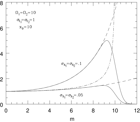
FIG. 1.: Plot of the “incoherent probability” ${\cal P}_{\rm incoh}$ (Eq. (44), normalized to its value at $m$$=$$0$) as a function of mass for the case of a single neutrino, taking $\sigma_{x_{1,2}}$$=$$0.1,0.05$. In each case, the solid line shows the exact result and the dashed line shows the result obtained in the approximation of Eq. (46). The dash-dotted line shows a plot of $1/v(m)$ for comparison.

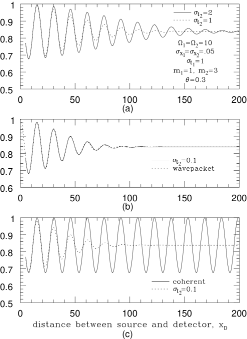
FIG. 2.: Oscillation probabilities as a function of distance. The two curves in (a) correspond to the “incoherent” detector with time resolutions $\sigma_{t_{2}}$$=$$1,2$. The solid curve in (b) gives the “incoherent” probability for $\sigma_{t_{2}}$$=$$0.1$. The dotted curve shows the analogous result obtained in the wave packet approach. The solid curve in (c) shows the probability measured by the “coherent” detector.

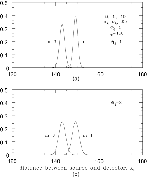
FIG. 3.: “Snapshots” of two mass eigenstate wave packets using incoherent detectors with different time resolutions. The wave packets have been individually normalized over $x_{D}$. In (a) the time resolution of the detector is such that the wave packets appear to be nearly separated, while in (b) the same wave packets appear to overlap due to the broader temporal resolution in that case.

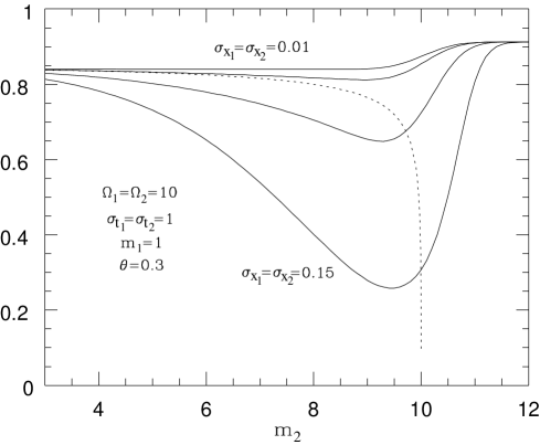
FIG. 4.: Plot of the constant flavour-conserving probability, ${\cal P}^{\infty}_{e\rightarrow e}$, defined in Eq. (76) as a function of the mass of the heavier neutrino. The solid lines correspond to spatial widths $\sigma_{x_{1,2}}$$=$$0.01,0.05,0.1,0.15$ and the dotted line shows the value obtained in the wave packet approach if the contributions corresponding to the various mass eigenstates are weighted by $1/v_{i}$.

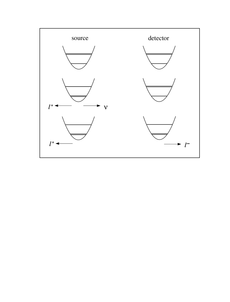
FIG. 5.: A schematic illustration of the sequence of events in the source/detector system for fermionic neutrinos considered in Sec. III. The excited source decays by emitting a neutrino and its associated anti-lepton. The detector subsequently absorbs the neutrino and emits a lepton.

FIG. 6.: Plot of the two functions $h^{+}_{e\rightarrow e}$ and $h^{-}_{e\rightarrow e}$ as a function of the neutrino mass. These provide a measure of the probability to produce lepton pairs with helicity $+1$ and $-1$, for $h^{+}$ and $h^{-}$, respectively.

REFERENCES

-
[1]
See, for example, R. Adler et al. (CPLEAR Collaboration),
Phys. Lett. B 363 (1995) 237;
Phys. Lett. B 363 (1995) 243;
D. Buskulic et al. (ALEPH Collaboration), Z. Phys. C 75 (1997) 397. - [2] B. Pontecorvo, Sov. Phys. JETP 26 (1968) 984.
- [3] L. Wolfenstein, Phys. Rev. D 17 (1978) 2369; Phys. Rev. D 20 (1979) 2634.
- [4] S.P. Mikheyev and A. Yu. Smirnov, Yad. Fiz. 42 (1985) 1441 [Sov. J. Nucl. Phys. 42 (1985) 913]; Il Nuovo Cimento C 9 (1986) 17.
- [5] N. Arkani-Hamed, J.L. Feng, L.J. Hall and H.-C. Cheng, hep-ph/9704205, and references therein.
- [6] B. Kayser, Phys. Rev. D 24 (1981) 110.
- [7] S. Nussinov, Phys. Lett. B 63 (1976) 201.
- [8] C. Giunti, C.W. Kim and U.W. Lee, Phys. Rev. D 44 (1991) 3635.
- [9] C. W. Kim and A. Pevsner, “Neutrinos in Physics and Astrophysics,” Contemporary Concepts in Physics, Vol. 8, edited by H. Feshbach (Harwood Acad. Publishers, Chur, 1993).
- [10] C.W. Kim, C. Giunti and U.W. Lee, Nucl. Phys. B (Proc. Suppl.) 28A (1992) 172.
- [11] B. Ancochea, A. Bramon, R. Muñoz-Tapia and M. Nowakowski, Phys. Lett. B 389 (1996) 149.
- [12] K.A. Kiers, Ph.D. thesis, University of British Columbia, 1996.
-
[13]
Y.N. Srivastava, A. Widom and E. Sassaroli,
Phys. Lett. B 344 (1995) 436;
Z. Phys. C 66 (1995) 601; hep-ph/9507330; hep-ph/9511294;
S. Mohanty, hep-ph/9702428 (see, however, S. Mohanty, hep-ph/9706328). - [14] H. Lipkin, Phys. Lett. B 348 (1995) 604.
- [15] Y. Grossman and H. Lipkin, Phys. Rev. D 55 (1997) 2760; hep-ph/9606315.
- [16] J. Lowe, B. Bassalleck, H. Burkhardt, A. Rusek, G.J. Stephenson Jr. and T. Goldman, Phys. Lett. B 384 (1996) 288.
- [17] B. Kayser, in the Proceedings of the 28th International Conference on High Energy Physics, (World Scientific, Warsaw, 1996), hep-ph/9702327; “The Frequency of Neutral Meson and Neutrino Oscillation,” SLAC-PUB-7123.
- [18] K. Kiers, S. Nussinov and N. Weiss, Phys. Rev. D 53 (1996) 537.
- [19] C. Giunti, C.W. Kim, J.A. Lee and U.W. Lee, Phys. Rev. D 48 (1993) 4310.
- [20] W. Grimus and P. Stockinger, Phys. Rev. D 54 (1996) 3414.
- [21] J. Rich, Phys. Rev. D 48 (1993) 4318.
- [22] C. Giunti, C.W. Kim and U.W. Lee, hep-ph/9709494.
- [23] See, for example, W. G. Unruh and R. M. Wald, Phys. Rev. D 29 (1984) 1047.
- [24] This connection has also been noted in Ref. [20].
- [25] C. Giunti, C.W. Kim and U.W. Lee, Phys. Rev. D 45 (1992) 2414.
- [26] C. Itzykson and J.-B. Zuber, “Quantum Field Theory,” (McGraw-Hill Inc., New York, 1980).