Light-Cone Quantized QCD and Novel Hadron Phenomenology

I review progress made in solving gauge theories such as collinear quantum chromodynamics using light-cone Hamiltonian methods. I also show how the light-cone Fock expansion for hadron wavefunctions can be used to compute operator matrix elements such as decay amplitudes, form factors, distribution amplitudes, and structure functions, and how it provides a tool for exploring novel features of QCD. I also review commensurate scale relations, leading-twist identities which relate physical observables to each other, thus eliminating renormalization scale and scheme ambiguities in perturbative QCD predictions.

1 Introduction

The key challenge of nonperturbative quantum chromodynamics is to compute the spectrum of hadrons and gluonic states from first principles as well as determine the wavefunctions for each QCD bound state in terms of its quark and gluon degrees of freedom. If we had such a complete solution, then we could compute the quark and gluon structure functions and distribution amplitudes which control hard-scattering inclusive and exclusive reactions, as well as all of the operator matrix elements of currents which underlie electro-weak form factors and the weak decay amplitudes of the light and heavy hadrons. The knowledge of hadron wavefunctions would also provide a deep understanding of the physics of QCD at the amplitude level, illuminating exotic effects of the theory such as color transparency, intrinsic heavy quark effects, hidden color, diffractive processes, and the QCD van der Waals interactions.

Solving a quantum field theory such as QCD is clearly not easy. However, highly non-trivial, one-space one-time relativistic quantum field theories which mimic many of the features of QCD have already been completely solved using light-cone Hamiltonian methods.$\!{}^{{\bf?}}$ In fact, virtually any (1+1) quantum field theory can be solved using the method of Discretized Light-Cone-Quantization (DLCQ). $\!{}^{{\bf?},{\bf?}}$ In DLCQ, a quantum field theory is rendered discrete in momentum space by imposing periodic or anti-periodic boundary conditions. The Hamiltonian $H_{LC}$, which can be constructed from the Lagrangian using light-cone time quantization, can then be diagonalized, in analogy to Heisenberg’s solution of the eigenvalue problem in quantum mechanics. In the one-space one-time theories, the diagonalization is a straightforward computational problem, and the resulting eigenvalues and eigensolutions then provide the complete spectrum of hadrons, together with their respective light-cone wavefunctions.

A beautiful illustration of the application of light-cone quantization to the solution of a quantum field theory is the DLCQ analysis of “collinear” QCD: a variant of $QCD(3+1)$ defined by dropping all of interaction terms in $H^{QCD}_{LC}$ involving transverse momenta.$\!{}^{{\bf?}}$ Even though this theory is effectively two-dimensional, the transversely-polarized degrees of freedom of the gluon field are retained as two scalar fields. Antonuccio and Dalley $\!{}^{{\bf?}}$ have recently used DLCQ to solve this theory. The diagonalization of $H^{\rm collinear}_{LC}$ provides not only the complete bound and continuum spectrum of the collinear theory, but it also yields the complete ensemble of light-cone Fock state wavefunctions needed to construct the quark and gluon structure functions of each hadronic and gluonic state. For example, Antonuccio and Dalley obtain the spectrum of gluonia, and the polarized gluon and quark structure functions of the mesonic states. Although the collinear theory is a drastic approximation to physical $QCD(3+1)$, the phenomenology of its DLCQ solutions demonstrate general features of gauge theory, such as the peaking of the wavefunctions at minimal invariant mass, color coherence, and the helicity retention of leading partons in the polarized structure functions at $x\rightarrow 1$. The DLCQ solutions of the one-space one-time gauge theories can be obtained for arbitrary coupling strength, flavors, and colors.

The solutions to collinear QCD provide a “standard candle” or theoretical laboratory in which other nonperturbative methods proposed to solve QCD, such as lattice gauge theory, Bethe-Salpeter methods, and various approximations can be tested and compared.

The fact that one actually solve a non-trivial relativistic quantum field theory in one space and one time gives hope that the full solutions to QCD(3+1) will eventually be accomplished. In these lectures I shall also discuss the possibility that one can use the collinear theory as a first approximation to a procedure which systematically constructs the full wavefunction solutions of QCD(3+1). I will also outline the progress made in understanding hadrons at the amplitude level, using the light-cone Fock expansion as a physics tool for exploring novel features of QCD in hadron physics. I also review commensurate scale relations, a method which relates physical observables to each other, thus eliminating ambiguities due to scale and scheme ambiguities.

2 The Light-Cone Fock Expansion

The concept of the “number of constituents” of a relativistic bound state such as a hadron in quantum chromodynamics, is not only frame-dependent, but its value can fluctuate to an arbitrary number of quanta. Thus when a laser beam crosses a proton at fixed “light-cone” time $\tau=t+z/c=x^{0}+x^{z}$, an interacting photon can encounter a state with any given number of quarks, anti-quarks, and gluons in flight (as long as $n_{q}-n_{\overline{q}}=3$). The probability amplitude for each such $n$-particle state of on-mass shell quarks and gluons in a hadron is given by a light-cone Fock state wavefunction $\psi_{n/H}(x_{i},\vec{k}_{\perp i},\lambda_{i})$, where the constituents have positive longitudinal light-cone momentum fractions

$$x_{i}=\frac{k^{+}_{i}}{P^{+}}=\frac{k^{0}+k^{z}_{i}}{P^{0}+P^{z}}\ ,\quad\sum^{n}_{i=1}x_{i}=1\ ,$$ (1)

relative transverse momentum

$$\vec{k}_{\perp i}\ ,\quad\sum^{n}_{i=1}\vec{k}_{\perp i}=\vec{0}_{\perp}\ ,$$ (2)

and helicities $\lambda_{i}.$ The ensemble {$\psi_{n/H}$} of such light-cone Fock wavefunctions is a key concept for hadron physics, providing a conceptual basis for representing physical hadrons (and also nuclei) in terms of their fundamental quark and gluon degrees of freedom.$\!{}^{{\bf?}}$ In the light-cone formalism, the vacuum is essentially trivial. Since each particle moves forward in light-cone time $\tau$ with positive light-cone momenta fractions $x_{i}$, light-cone perturbation theory is particularly simple and intuitive, involving many fewer diagrams than equal-time theory.

The light-cone Fock expansion is defined in the following way: one first constructs the light-cone time evolution operator $P^{-}=P^{0}-P^{z}$ and the invariant mass operator $H_{LC}=P^{-}P^{+}-P^{2}_{\perp}$ in light-cone gauge $A^{+}=0$ from the QCD Lagrangian. The total longitudinal momentum $P^{+}=P^{0}+P^{z}$ and transverse momenta $\vec{P}_{\perp}$ are conserved, i.e., are independent of the interactions. The matrix elements of $H_{LC}$ on the complete orthonormal basis $\{|n>\}$ of the free theory $H^{0}_{LC}=H_{LC}(g=0)$ can then be constructed. The matrix elements $\left\langle{n\,|\,H_{LC}\,|\,m}\right\rangle$ connect Fock states differing by 0, 1, or 2 quark or gluon quanta, and they include the instantaneous quark and gluon contributions imposed by eliminating dependent degrees of freedom in light-cone gauge.

In practice it is essential to introduce an ultraviolet regulator in order to limit the total range of $\left\langle{n\,|\,H_{LC}\,|\,m}\right\rangle$, such as a “global” cutoff in the invariant mass of the free Fock states:

$${\cal M}^{2}_{n}=\sum^{n}_{i=1}\frac{k^{2}_{\perp}+m^{2}}{x}<\Lambda^{2}_{\rm global}\ .$$ (3)

One can also introduce a “local” cutoff to limit the change in invariant mass $|{\cal M}^{2}_{n}-{\cal M}^{2}_{m}|<\Lambda^{2}_{\rm local}$ which provides spectator-independent regularization of the sub-divergences associated with mass and coupling renormalization.

The natural renormalization scheme for the coupling is $\alpha_{V}(Q)$, the effective charge defined from the scattering of two infinitely heavy quark test charges. The renormalization scale can then be determined from the virtuality of the exchanged momentum, as in the BLM and commensurate scale methods.$\!{}^{{\bf?},{\bf?}}$ I will discuss this further in Section 18.

In the DLCQ method , the matrix elements $\left\langle{n\,|\,H^{(\Lambda)}_{LC}\,|\,m}\right\rangle$, are made discrete in momentum space by imposing periodic or anti-periodic boundary conditions in $x^{-}=x^{0}-x^{z}$ and $\vec{x}_{\perp}$ (see Section 3). Upon diagonalization of $H_{LC}$, the eigenvalues provide the invariant mass of the bound states and eigenstates of the continuum. The projection of the hadronic eigensolutions on the free Fock basis define the light-cone wavefunctions. For example, for the proton,

$$\,\left|\,{p}\right\rangle = \sum_{n}\left\langle{n\,|\,p}\right\rangle\,\,\left|\,{n}\right\rangle$$

$$= \psi^{(\Lambda)}_{3q/p}(x_{,}\vec{k}_{\perp i},\lambda_{i})\,\,\left|\,{uud}\right\rangle$$

$$+\psi^{(\Lambda)}_{3qg/p}(x_{i},\vec{k}_{\perp i},\lambda_{i})\,\,\left|\,{uudg}\right\rangle+\cdots$$

The light-cone formalism has the remarkable feature that the $\psi^{(\Lambda)}_{n/H}(x_{i},\vec{k}_{\perp i},\lambda_{c})$ are invariant under longitudinal boosts; i.e., they are independent of the total momentum $P^{+}$, $\vec{P}_{\perp}$ of the hadron. As we shall discuss below, given the $\psi^{(\Lambda)}_{n/H},$ we can construct any electromagnetic or electroweak form factor from the diagonal overlap of the LC wavefunctions.$\!{}^{{\bf?}}$ This is illustrated in detail in Section 6. Similarly, the matrix elements of the currents that define quark and gluon structure functions can be computed from the integrated squares of the LC wavefunctions.$\!{}^{{\bf?}}$

These properties of the LC formalism are all highly-nontrivial features. In contrast, in equal-time formalism, the evaluation of any electromagnetic form factor requires the computation of non-diagonal matrix elements of bound state Fock wavefunctions in which the parton number can change by two units; even worse, matrix elements involving spontaneous pair production or annihilation is also required, so a complete solution of the vacuum is also required. In light-cone quantization, the full vacuum is also the vacuum of the free theory and thus is trivial. Further, the equal-time computation is only valid in one Lorentz frame; boosting the result to a different frame is a dynamical problem as complicated as solving the complete Hamiltonian problem itself.

In general, any hadronic amplitude such as quarkonium decay, heavy hadron decay, or any hard exclusive hadron process can be constructed as the convolution of the light-cone Fock state wavefunctions with quark-gluon matrix elements $\!{}^{{\bf?}}$

$${\cal M}_{\rm Hadron} = \prod_{H}\sum_{n}\int\prod^{n}_{i=1}d^{2}k_{\perp}\prod^{n}_{i=1}dx\,\delta\left(1-\sum^{n}_{i=1}x_{i}\right)\,\delta\left(\sum^{n}_{i=1}\vec{k}_{\perp i}\right)$$ (5)

$$\times\psi^{(\Lambda)}_{n/H}(x_{i},\vec{k}_{\perp i},\Lambda_{i})\,{\cal M}^{(\Lambda)}_{q,g}\ .$$

Here ${\cal M}^{(\Lambda)}_{q,g}$ is the underlying quark-gluon subprocess scattering amplitude, where the (incident or final) hadrons are replaced by quarks and gluons with momenta $x_{i}p^{+}$, $x_{i}\vec{p}_{\perp}+\vec{k}_{\perp i}$ and invariant mass above the separation scale ${\cal M}^{2}_{n}>\Lambda^{2}$. The LC ultraviolet regulators thus provide a LC factorization scheme for elastic and inelastic scattering, separating the hard dynamical contributions with invariant mass squared ${\cal M}^{2}>\Lambda^{2}_{\rm global}$ from the soft physics with ${\cal M}^{2}\leq\Lambda^{2}_{\rm global}$ which is incorporated in the nonperturbative LC wavefunctions. The DGLAP evolution of parton distributions can be derived by computing the variation of the Fock expansion with respect to $\Lambda^{2}_{\rm global}$.$\!{}^{{\bf?}}$

The use of the global cutoff to separate hard and soft physics is more than a convention; it is essential in order to correctly analyze the behavior of deep inelastic scattering structure functions in the $x_{bj}\to 1$ endpoint regime.$\!{}^{{\bf?}}$ At large $x$, the spectator constituents of the hadron target are forced to stop, placing the struck quark far off shell. From the stand-point of the LC Hamiltonian theory, the LC energy $M^{2}-{\cal M}_{n}^{2}$ becomes infinitely negative. Similarly, in the covariant formalism, the Feynman virtuality becomes infinitely spacelike: $k_{F}^{2}-m_{q}^{2}=(p-p_{s})^{2}-m_{s}^{2}=-x(M^{2}-{\cal M}_{n}^{2})\to-(m_{s}^{2}+k^{2}_{\perp})/(1-x)$ for $x\to 1$. Here $x$ is the light-cone momentum fraction of the light quark, $p_{s}$ is the four-momentum of the remnant spectator system with $p^{2}_{s}=m^{2}_{s}>0.$ Thus in the large $x$ regime, where $k_{F}^{2}$ becomes far off-shell, one cannot separate the hard physics from the physics of the target wavefunction. The LC factorization scheme correctly isolates this phenomena. An important physical consequence is that DGLAP evolution is truncated; effectively, the starting evolution scale is of order $-k^{2}_{F}$. Thus in the $x_{Bj}\sim 1$ regime where $W^{2}=(p+q)^{2}=(1-x_{Bj})Q^{2}/x_{bj}$ is fixed, the DGLAP evolution due to the radiation of hard gluons is truncated and the power law behavior $(1-x_{Bj})^{n}$ dictated by the underlying hadron wavefunctions is maintained. It is this fact which allows exclusive-inclusive duality in deep inelastic lepton scattering to be maintained: the nominal power law (dimensional counting) behavior of structure functions at $x\to 1$ and the power-law fall off of form factors at large $Q^{2}$ match at fixed $W^{2}$.

The simplest, but most fundamental, characteristic of a hadron in the light-cone representation, is the hadronic distribution amplitude,$\!{}^{{\bf?}}$ defined as the integral over transverse momenta of the valence (lowest particle number) Fock wavefunction; e.g., for the pion

$$\phi_{\pi}(x_{i},Q)\equiv\int d^{2}k_{\perp}\,\psi^{(Q)}_{q\overline{q}/\pi}(x_{i},\vec{k}_{\perp i},\lambda)$$ (6)

where the global cutoff $\Lambda_{global}$ is identified with the resolution $Q$. The distribution amplitude controls leading-twist exclusive amplitudes at high momentum transfer, and it can be related to the gauge-invariant Bethe-Salpeter wavefunction at equal light-cone time $\tau=x^{+}$. The distribution amplitude is boost and gauge invariant. Its $\log Q$ evolution can be derived from the perturbatively-computable tail of the valence light-cone wavefunction in the high transverse momentum regime.$\!{}^{{\bf?},{\bf?}}$

Exclusive processes are particularly challenging to compute in quantum chromodynamics because of their sensitivity to the unknown nonperturbative bound state dynamics of the hadrons. However, in some important cases, the leading power-law behavior of an exclusive amplitude at large momentum transfer can be computed rigorously in the form of a factorization theorem which separates the soft and hard dynamics. For example, the leading $1/Q^{2}$ fall-off of the meson form factors can be computed as a perturbative expansion in the QCD coupling$\!{}^{{\bf?},{\bf?}}$:

$$F_{M}(Q^{2})=\int^{1}_{0}dx\int^{1}_{0}dy\phi_{M}(x,{\tilde{Q}})T_{H}(x,y,Q^{2})\phi_{M}(y,{\tilde{Q}}),$$ (7)

where $\phi_{M}(x,{\tilde{Q}})$ is the process-independent meson distribution amplitude which encodes the nonperturbative dynamics of the bound valence Fock state up to the resolution scale ${\tilde{Q}}$, and

$$T_{H}(x,y,Q^{2})=16\pi C_{F}{\alpha_{s}(\mu)\over(1-x)(1-y)Q^{2}}\left(1+O(\alpha_{s})\right)$$ (8)

is the leading-twist perturbatively calculable subprocess amplitude $\gamma^{*}q(x)\overline{q}(1-x)\to q(y)\overline{q}(1-y)$, obtained by replacing the incident and final mesons by valence quarks collinear up to the resolution scale ${\tilde{Q}}$. The contributions from non-valence Fock states and the correction from neglecting the transverse momentum in the subprocess amplitude from the nonperturbative region are higher twist, i.e., they are power-law suppressed. The transverse momenta in the perturbative domain lead to the evolution of the distribution amplitude and to next-to-leading-order (NLO) corrections in $\alpha_{s}$. The contribution from the endpoint regions of integration, $x\sim 1$ and $y\sim 1,$ are power-law and Sudakov suppressed and thus can only contribute corrections at higher order in $1/Q$.$\!{}^{{\bf?}}$

The physical pion form factor must be independent of the separation scale $\tilde{Q}.$ Again, it should be emphasized that the natural variable to make this separation is the light-cone energy, or equivalently the invariant mass ${\cal M}^{2}={\vec{k_{\perp}}^{2}/x(1-x)}$, of the off-shell partonic system.$\!{}^{{\bf?},{\bf?}}$ Any residual dependence on the choice of $\tilde{Q}$ for the distribution amplitude will be compensated by a corresponding dependence of the NLO correction in $T_{H}.$ However, the NLO prediction for the pion form factor depends strongly on the form of the pion distribution amplitude as well as the choice of renormalization scale $\mu$ and scheme. I will discuss recent progress in eliminating such scheme and scale ambiguities and testing QCD in exclusive processes in Sections 18 and 19.

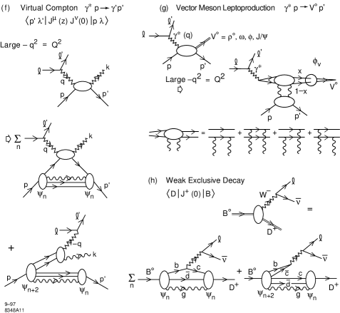
Figure 1: Computation of QCD processes in terms of light-cone Fock wavefunctions. The various processes are described in the text.

A catalog of applications of light-cone Fock wavefunctions to QCD processes is illustrated in Fig. 1. The light-cone expansion for a proton in terms of the complete set of color-singlet baryon number $B=1$ free Fock states is illustrated in Fig. 1a. The distribution amplitude which controls high momentum transfer mesonic processes is illustrated in Fig. 1b. The meson distribution amplitude $\phi_{M}(x,Q)$ is defined such that the invariant mass ${\cal M}$ of the free partons in any intermediate state are cutoff at the ultraviolet scale $Q$. The relation of structure functions in deep inelastic lepton scattering to the integrated square of light-cone Fock wavefunctions is illustrated in Fig. 1c. As shown in Fig. 1d, the light-cone wavefunctions provide an exact basis for the computation of the matrix elements of spacelike local currents in terms of diagonal overlap integrals with $x_{i}=x_{i}^{\prime}$ unchanged and parton number $n=n^{\prime}$. Figure 1d also illustrates the factorization of the nucleon form factors at high momentum transfer in terms of the convolution of a hard-scattering amplitude $T_{H}(x_{i},y_{i},Q)$ (for the scattering the valence quarks from the initial to final direction) with the nucleon distribution amplitudes. Figure 1e illustrates the application of perturbative QCD factorization to the Compton scattering amplitude at large $-t$ and $s$. Figure 1f illustrates the computation of a non-forward matrix element of currents; specifically virtual Compton scattering where the incident photon has large incident virtuality $q^{2}=-Q^{2}$. Non-diagonal $n^{\prime}=n-2$ Fock state convolutions are required when evaluating such processes in a collinear reference frame. The computation of a weak decay matrix element $B^{0}\to D^{+}\ell\overline{\nu}$ in terms of light-cone Fock wavefunctions is illustrated in Fig. 1g. Both diagonal and non-diagonal overlap integrals contribute. Finally, the perturbative QCD factorization of the dominant contribution to vector meson leptoproduction at large photon virtuality $Q^{2}$ and high energy $s\gg-t,Q^{2}$ is illustrated in Fig. 1h. The dominant contribution arises from longitudinally polarized photons, and the $q\overline{q}$ pair typically has small transverse size $b_{\perp}\sim 1/Q$. The coupling of the quark pair to the outgoing vector meson is controlled by the vector meson distribution amplitude.

3 DLCQ: A Program for Solving QCD (3+1).

The DLCQ method $\!{}^{{\bf?}}$ consists of diagonalizing the light-cone Hamiltonian at fixed $x^{+}$ on a free Fock basis $\{\,\left|\,{n}\right\rangle\}$; i.e. the complete set of eigenstates of the free Hamiltonian $H^{0}_{LC}$ satisfying periodic or anti-periodic boundary conditions in $x^{-}$. The eigenvalue problem is

$$H_{LC}\,\left|\,{\Psi}\right\rangle = M^{2}\,\left|\,{\Psi}\right\rangle$$ (9)

$$\left\langle{n\,|\,H_{LC}\,|\,m}\right\rangle\left\langle{m\,|\,\Psi}\right\rangle = M^{2}\left\langle{n\,|\,\Psi}\right\rangle$$ (10)

with

$$k^{+}_{i}=\frac{2\pi}{L}\,n_{i}>0\qquad P^{+}=\frac{2\pi}{L}\,K\qquad\Sigma n_{i}=K\ .$$ (11)

Here $K$, the “harmonic resolution,” is an arbitrary positive integer. The continuum limit corresponds to $K\Rightarrow\infty$. The value of length $L$ is an irrelevant boost parameter in that it never appears in physics results. Since there are only a finite number of partitions of a given $K$ among the positive integers $n_{i}$ with $\Sigma n_{i}=K$, the number of distribution Fock states are automatically rendered discrete. The transverse momenta are also made discrete by choosing periodic or anti-periodic conditions in $x_{\perp}$. Then

$$\vec{k}_{\perp i}=\frac{2\pi}{L_{\perp}}\ \vec{n}_{\perp i}\ .$$ (12)

The limit on the number of states is then controlled by the global cutoff.

The diagonalization of the light-cone Hamiltonian thus becomes the problem of diagonalizing large Hermitian matrices, a numerical analysis problem, solvable by Lanczos or other methods. In the case of 1+1 dimensions, the problem is completely tractable, so virtually any 1+1 quantum field theory can be solved in this manner.

In the case of QCD (1+1) in $A^{+}=0$ gauge, where there are no dynamical gluons, the only interaction terms arise from “instantaneous” gluon exchange:

$$H^{LC}_{I}=\frac{g^{2}}{\pi}\left[\frac{1}{(k^{+}-\ell^{+})^{2}}-\frac{1}{(k^{+}+m^{+})^{2}}\right]$$ (13)

corresponding to $t$-channel or $s$-channel contributions in the amplitude

$$\overline{q}(k^{+})\,q(m^{+})+\overline{q}(\ell^{+})\,q(n^{+})\ .$$ (14)

There is also a mass renormalization contribution to $q(n^{+})$ generated from normal ordering

$$\delta H=\frac{g^{2}}{\pi}\ \sum^{n^{+}}_{m=1}\ \frac{1}{m^{2}}\ .$$ (15)

The solution to the diagonalization of the light-cone Hamiltonian produces not only the mass eigenvalues of the theory, but also the eigensolutions, as wavefunction coefficients in the LC Fock basis:

$$\,\left|\,{\Psi}\right\rangle=\sum_{n}\psi_{n}(x_{i},\vec{k}_{\perp i},\lambda_{i})\,\left|\,{n}\right\rangle$$ (16)

where each Fock component $\,\left|\,{n}\right\rangle$ has the same global and conserved quantum numbers as the eigenstate. The values of the light-cone momentum fractions are evaluated at

$$x^{+}_{i}=\frac{k^{+}_{i}}{p^{+}}=\frac{n_{i}}{K}=\left\{\frac{1}{K}\,,\frac{2}{K}\,,\frac{3}{K}\,\cdots\frac{K-1}{K}\right\}\$$ (17)

Thus one samples the wavefunctions at rational points which approach the continuum theory at $K\rightarrow\infty$. The absence of the end-points at $x_{i}=0,1$ corresponds to the neglect of zero modes. Except for massless, collinear $k_{1}$, such parton configurations are associated with infinitely massive free energy:

$${\cal M}^{2}_{n}=\sum^{n}_{i=1}\,\left(\frac{k^{2}_{\perp}+m^{2}}{x}\right)_{i}\rightarrow\infty$$ (18)

and thus exceed the global cutoff limit. Physically, the $x\rightarrow 0$ limit is associated with partons infinitely far in rapidity from the center of mass of the bound state itself

$$y_{i}-Y=\ell n\,x_{i}\ ;$$ (19)

such partons are only relevant at very large energies $W^{2}=(p+q)^{2}$ in the computation of structure functions. On the other hand, the LC Fock wavefunctions do not necessarily vanish at $x_{i}=0$ since they may correspond to soft gluons with $m^{2}$ and $k^{2}_{\perp}=0$. In general, even the fermion distribution need not vanish at $x\rightarrow 0$ in gauge theory since only the combination from the sum over states,

$$\sum\left[\frac{(\vec{k}_{\perp}-g\,\vec{A}_{\perp})^{2}+m^{2}}{x}\right]_{i}$$ (20)

has to be finite in the interacting theory. As Antonuccio and Dalley and I $\!{}^{{\bf?}}$ have recently shown, the cancellation of infinities at $x_{i}\rightarrow 0$ for fermions in gauge theory imposes strict “ladder relations” between Fock states with one or two more or less gluons in the bound state. We have also shown how this type of analysis leads to Regge power-law behavior of the quark distributions at $x\rightarrow 0$.

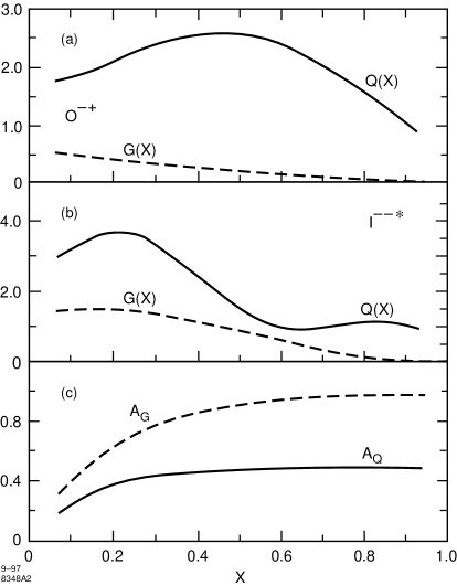
Figure 2: Examples of quark and gluon distributions in meson bound states in collinear QCD. From Antonuccio and Dalley.$\!{}^{{\bf?}}$ (a) Lowest $J_{z}=0$ mesonic state; (b) excited $J_{z}=1$ mesonic state; (c) longitudinal helicity asymmetry in lowest $J_{z}=1$ mesonic state.

These interesting features are illustrated in Fig. 2a and 2b which shows the gluon $G(x)$ and quark $Q(x)$ distributions of the lowest $0^{-+}$ and first excited $1^{--}$ mesonic bound states of collinear QCD $(N_{c}\rightarrow\infty)$ from DLCQ.$\!{}^{{\bf?}}$ Neither the quark nor the gluon distributions vanish at $x\rightarrow 0$. The polarization asymmetry for quarks and gluons with helicity aligned and anti-aligned to the $J_{z}$ spin of $1^{--}$ ground state shown in Fig. 2c demonstrates the tendency toward helicity alignment at $x\rightarrow 1$.

4 Jet Hadronization in Light-Cone QCD

One of the goals of nonperturbative analysis in QCD is to compute jet hadronization from first principles. The DLCQ solutions provide a possible method to accomplish this. By inverting the DLCQ solutions, we can write the “bare” quark state of the free theory as

$$\,\left|\,{q_{0}}\right\rangle=\sum\,\left|\,{n}\right\rangle\left\langle{n\,|\,q_{0}}\right\rangle$$ (21)

where now $\{\,\left|\,{n}\right\rangle\}$ are the exact DLCQ eigenstates of $H_{LC}$, and $\left\langle{n\,|\,q_{0}}\right\rangle$ are the DLCQ projections of the eigensolutions. The expansion in automatically infrared and ultraviolet regulated if we impose global cutoffs on the DLCQ basis:

$$\lambda^{2}<\Delta{\cal M}^{2}_{n}<\Lambda^{2}\ .$$ (22)

where $\Delta{\cal M}^{2}_{n}={\cal M}^{2}_{n}-(\Sigma{\cal M}_{i})^{2}$. It would be interesting to study this type of jet hadronization at the amplitude level for the existing DLCQ solutions to QCD (1+1) and collinear QCD.

5 Light-Cone Quantization and Renormalization Theory

The renormalization procedure for LC Hamiltonian theory is well understood in perturbation theory. For example, mass and coupling renormalization counter terms can be introduced in the standard way in QED to absorb the ultraviolet divergences at each order of perturbation theory. An explicit method, “alternating denominators”, which provides an automatic method to construct the local counter terms, was used$\!{}^{{\bf?}}$ to compute the lepton anomalous moments through order $\alpha^{2}$ and partly through order $\alpha^{3}.$ Lepage and I have employed an ultraviolet Hamiltonian renormalization scheme to derive the hard-scattering expansion for exclusive processes in QCD, including the evolution equations for the renormalized distribution amplitudes. Burkardt and Langnau$\!{}^{{\bf?}}$ have shown that kinetic and vertex mass renormalization counter terms are needed to restore the full invariance structure of the theory when one uses a light-cone regulation such as the global cutoff. Burkardt$\!{}^{{\bf?}}$ also has shown that tadpole diagram renormalization of $g\phi^{4}$ theory is consistently handled in the LC theory as a zero mode component to the renormalization of the scalar particles. The renormalization of Yukawa theories has also been analyzed.$\!{}^{{\bf?}}$ Hiller, McCartor, and I are working on a program in which the full Lorentz-invariant structure of light-cone Hamiltonian theory is restored using generalized Pauli-Villars regularization.

One of the advantages of DLCQ is that it provides a convenient infrared regularization of zero modes since they become discrete entities. In some model field theories, the zero modes take the place of the vacuum in reproducing the physics of spontaneous symmetry breaking. In other cases, such as the massive Schwinger model QED (1+1), the zero modes allow a simulation of external electric fields. As yet it is not clear whether LC zero roles play an essential role in analyzing QCD(3+1).

6 Form Factors and Light-Cone Wavefunctions

A critical advantage of the light-cone formalism is that the knowledge of the LC Fock wavefunction is sufficient to compute the elastic electroweak form factors. It is remarkable that all such matrix elements can be computed from diagonal (parton-conserving) overlap integrals of the LC Fock wavefunctions. In this section I will review the light-cone formalism for the computation of form factors for both elementary and composite systems.$\!{}^{{\bf?},{\bf?},{\bf?}}$ We can choose light-cone coordinates with the incident lepton directed along the $z$ direction$\!{}^{{\bf?}}$ $(p^{\pm}\equiv p^{0}\pm p^{3})$:

$$p^{\mu}\equiv(p^{+},p^{-},\overrightarrow{\!\!p}_{1})=\left(p^{+},\frac{M^{2}}{p^{+}},\overrightarrow{\!\!0}\!\!_{\perp}\right)\ ,\qquad q=\left(0,\frac{2q\cdot p}{p^{+}},\overrightarrow{\!\!q}\!\!_{\perp}\right)\ ,$$ (23)

where $q^{2}=-2q\cdot p=-q^{2}\!\!_{\perp}$ and $M=m_{\ell}$ is the mass of the composite system. The Dirac and Pauli form factors can be identified$\!{}^{{\bf?},{\bf?}}$ from the spin-conserving and spin-flip current matrix elements $(J^{+}=J^{0}+J^{3})$:

$${\cal M}^{+}_{\uparrow\uparrow} = \left\langle p+q,\uparrow\left|\frac{J^{+}(0)}{p^{+}}\right|p,\uparrow\right\rangle=2F_{1}(q^{2})\ ,$$ (24)

$${\cal M}^{+}_{\uparrow\downarrow} = \left\langle p+q,\uparrow\left|\frac{J^{+}(0)}{p^{+}}\right|p,\uparrow\right\rangle=-2(q_{1}-iq_{2})\ \frac{F_{2}(q^{2})}{2M}\ ,$$ (25)

where $\uparrow$ corresponds to positive spin projection $S_{z}=+\frac{1}{2}$ along the $\widehat{z}$ axis.

Each Fock-state wave function $\left|n\right\rangle$ of the incident lepton is represented by the functions $\psi^{(n)}_{p,S_{z}}(x_{i},\vec{k}\!\!_{\perp i},S_{i})$, where

$$k^{\mu}\equiv(k^{+},k^{-},\vec{k}\!\!_{\perp})=\left(xp^{+},\,\frac{k^{2}_{\perp}+m^{2}}{xp^{+}},\vec{k}\!\!_{\perp}\right)$$

specifies the light-cone momentum coordinates of each constituent $i=1,\ldots,n$, and $S_{i}$ specifies its spin projection $S^{i}_{z}$. Momentum observation on the light cone requires

$$\sum^{n}_{i=1}k_{\perp i}=0\ ,\qquad\sum^{n}_{i=1}x_{i}=1\ ,$$

and thus $0<x_{i}<1$. The amplitude to find $n$ (on-mass-shell) constituents in the lepton is then $\psi^{(n)}$ multiplied by the spinor factors $u_{S_{i}}(k_{i})/(k^{+}_{i})^{-1/2}$ or $v_{S_{i}}(k_{i})/(k^{+}_{i})^{1/2}$ for each constituent fermion or anti-fermion. The Fock state is off the “energy shell”:

$$\left(p^{-}-\sum^{n}_{i=1}k^{-}_{i}\right)p^{+}=\sum^{n}_{i=1}\left(\frac{\vec{k}^{2}\!\!_{\perp i}+m^{2}_{i}}{x_{i}}\right)\ .$$

The quantity $(\vec{k}^{2}\!\!_{\perp i}+m^{2}_{i})/x_{i}$ is the relativistic analog of the kinetic energy $\vec{p}^{2}_{i}/2m_{i}$ in the Schrödinger formalism.

The wave function for the lepton directed along the final direction $p+q$ in the current matrix element is then

$$\psi^{(n)}_{p+q,S^{\prime}_{z}}(x_{i},\vec{k}^{\prime}\!\!_{\perp i},S^{\prime}_{i})\ ,$$

where$\!{}^{{\bf?}}$

$$\vec{k}^{\prime}\!\!_{\perp j}=\vec{k}\!\!_{\perp j}+(1-x_{j})\vec{q}\!\!_{\perp}$$

for the struck constituent and

$$\vec{k}^{\prime}\!\!_{\perp i}=\vec{k}\!\!_{\perp i}-x_{i}\vec{q}\!\!_{\perp}$$

for each spectator $(i\neq j)$. The $\vec{k}{}^{\prime}\!\!_{\perp}$ are transverse to the $p+q$ direction with

$$\sum^{n}_{i=1}\vec{k}^{\prime}\!\!_{\perp i}=0\ .$$

The interaction of the current $J^{+}(0)$ conserves the spin projection of the struck constituent fermion $(\overline{u}_{s},\gamma^{+}u_{s})/k_{+}=2\delta_{ss^{\prime}}$. Thus from Eqs. (24) and (25)

$$F_{1}(q^{2})=\frac{1}{2}{\cal M}^{+}_{\uparrow\uparrow}=\sum_{j}e_{j}\int[dx]\,\left[d^{2}\vec{k}\!\!_{\perp}\right]\,\psi^{*(n)}_{p+q,\uparrow}\left(x,\vec{k}^{\prime}\!\!_{\perp},S\right)\,\psi^{(n)}_{p,\uparrow}\left(x,\vec{k}\!\!_{\perp},S\right)\ ,$$ (26)

and

$$-\left(\frac{q_{1}-iq_{2}}{2M}\right)F_{1}(q^{2})=\frac{1}{2}{\cal M}^{+}_{\uparrow\downarrow}$$ (27)

$$= \sum_{j}e_{j}\int[dx]\,\left[d^{2}\vec{k}\!\!_{\perp}\right]\,\psi^{*(n)}_{p+q,\uparrow}\left(x,\vec{k}^{\prime}\!\!_{\perp},S\right)\,\psi^{(n)}_{p,\uparrow}\left(x,\vec{k}\!\!_{\perp},S\right)\ ,$$

where $e_{j}$ is the fractional charge of each constituent. [A summation of all possible Fock states $(n)$ and spins $(S)$ is assumed.] The phase-space integration is

$$[dx]\equiv\delta\left(1-\sum x_{i}\right)\prod^{n}_{i=1}dx_{i}\ ,$$ (28)

and

$$\left[d^{2}k_{\perp}\right]\equiv 16\pi^{3}\delta^{(2)}\left(\sum k_{\perp i}\right)\prod^{n}_{i=1}\frac{d^{2}k_{\perp}}{16\pi^{3}}\ .$$ (29)

Equation (26) evaluated at $q^{2}=0$ with $F_{1}(0)=1$ is equivalent to wavefunction normalization. The anomalous moment $a=F_{2}(0)/F_{1}(0)$ can be determined from the coefficient linear in $q_{1}-iq_{2}$ from the coefficient linear in $q_{1}-iq_{2}$ from $\psi^{*}_{p+q}$ in Eq. (27). In fact,

$$\frac{\partial}{\partial\vec{q}\!\!_{\perp}}\,\psi^{*}_{p+q}\equiv-\sum_{i\neq j}x_{i}\frac{\partial}{\partial\vec{k}\!\!_{\perp i}}\,\psi^{*}_{p+q}$$ (30)

(summed over spectators), we can, after integration by parts, write explicitly

$$\frac{a}{M}=-\sum_{j}e_{j}\int[dx]\int\left[d^{2}k_{\perp}\right]\sum_{i\neq j}\psi^{*}_{p\uparrow}x_{i}\left(\frac{\partial}{\partial k_{1i}}+i\frac{\partial}{\partial k_{2i}}\right)\psi_{p\downarrow}\ .$$ (31)

The wave function normalization is

$$\int[dx]\int\left[d^{2}k_{\perp}\right]\,\psi^{*}_{p\uparrow}\,\psi_{p\uparrow}=\int[dx]\int d^{2}k_{\perp}\psi^{*}_{p\downarrow}\,\psi_{p\downarrow}=1\ .$$ (32)

A sum over all contributing Fock states is assumed in Eqs. (31) and (32). We thus can express the anomalous moment in terms of a local matrix element at zero momentum transfer. It should be emphasized that Eq. (31) is exact; it is valid for the anomalous element of any spin-$\frac{1}{2}$ system.

In the case of the electron’s anomalous moment to order $\alpha$ in QED,$\!{}^{{\bf?},{\bf?}}$ the contributing intermediate Fock states are the electron-photon states with spins $\left|-\frac{1}{2},1\right\rangle$ and $\left|\frac{1}{2},-1\right\rangle$:

$$\psi_{p\downarrow}=\frac{e/\sqrt{x}}{M^{2}-\frac{k^{2}_{\perp}+\lambda^{2}}{x}-\frac{k^{2}_{\perp}+\widehat{m}^{2}}{1-x}}\times\left\{\begin{array}[]{l}\sqrt{2}\ \frac{(k_{1}-ik_{2})}{x}\ \left(\left|-\frac{1}{2}\right\rangle\rightarrow\left|-\frac{1}{2},1\right\rangle\right)\\[5.0pt] \sqrt{2}\ \frac{M(1-x)-\widehat{m}}{1-x}\ \left(\left|-\frac{1}{2}\right\rangle\rightarrow\left|\frac{1}{2},-1\right\rangle\right)\end{array}\right.$$ (33)

and

$$\psi^{*}_{p\uparrow}=\frac{e/\sqrt{x}}{M^{2}-\frac{k^{2}_{\perp}+\lambda^{2}}{x}-\frac{k^{2}_{\perp}+\widehat{m}^{2}}{1-x}}\times\left\{\begin{array}[]{l}-\sqrt{2}\ \frac{M(1-x)-\widehat{m}}{1-x}\ \left(\left|-\frac{1}{2},1\right\rangle\rightarrow\left|\frac{1}{2}\right\rangle\right)\\[5.0pt] -\sqrt{2}\ \frac{(k_{1}-ik_{2})}{x}\ \left(\left|\frac{1}{2},-1\right\rangle\rightarrow\left|\frac{1}{2}\right\rangle\right)\ .\end{array}\right.$$ (34)

The quantities to the left of the curly bracket in Eqs. (33) and (34) are the matrix elements of

$$\frac{\overline{u}}{(p^{+}-k^{+})^{1/2}}\,\gamma\cdot\epsilon^{*}\,\frac{u}{(p^{+})^{1/2}}\quad\hbox{and}\quad\frac{\overline{u}}{(p^{+})^{1/2}}\,\gamma\cdot\epsilon\,\frac{u}{(p^{+}-k^{+})^{1/2}}\ ,$$

respectively, where $\widehat{\epsilon}=\widehat{\epsilon}_{\uparrow(\downarrow)}=\pm(1/\sqrt{2})(\widehat{x}\pm i\widehat{y})$, $\epsilon\cdot k=0$, $\epsilon^{+}=0$ in the light-cone gauge for vector spin projection $S_{z}=\pm 1$.$\!{}^{{\bf?},{\bf?}}$ For the sake of generality, we let the intermediate lepton and vector boson have mass $\widehat{m}$ and $\lambda$, respectively.

Substituting (33) and (34) into Eq. (31), one finds that only the $\left|-\frac{1}{2},1\right\rangle$ intermediate state actually contributes to $a$, since terms which involve differentiation of the denominator of $\psi_{p\downarrow}$ cancel. We thus have$\!{}^{{\bf?}}$

$$a=4M\,e^{2}\int\frac{d^{2}k_{\perp}}{16\pi^{3}}\int^{1}_{0}dx\ \frac{\left[\widehat{m}-(1-x)M\right]/x(1-x)}{\left[M^{2}-(k^{2}_{\perp}+\widehat{m}^{2})/(1-x)-(k^{2}_{\perp}+\lambda^{2})/x\right]^{2}}\ ,$$ (35)

or

$$a=\frac{\alpha}{\pi}\int^{1}_{0}dx\ \frac{M\left[\widehat{m}-M(1-x)\right]x(1-x)}{\widehat{m}^{2}x+\lambda^{2}(1-x)-M^{2}x(1-x)}\ ,$$ (36)

which, in the case of QED $(\widehat{m}=M,\lambda=0)$ gives the Schwinger results $a=\alpha/2\pi$.

The general result (31) can also be written in matrix form:

$$\frac{a}{2M}=-\sum_{j}e_{j}\int[dx]\left[d^{2}k_{\perp}\right]\,\psi^{+}\overrightarrow{\!\!S}\!\!_{\perp}\cdot\overrightarrow{\!\!L}\!\!_{\perp}\psi\ ,$$ (37)

where $S$ is the spin operator for the total system and $\overrightarrow{\!\!L}\!\!_{\perp}$ is the generator of “Galiean” transverse boosts $\!{}^{{\bf?},{\bf?}}$ on the light cone, i.e., $\overrightarrow{\!\!S}\!\!_{\perp}\cdot\overrightarrow{\!\!L}\!\!_{\perp}=(S_{+}L_{-}+S_{-}L_{+})/2$ where $S_{\pm}=(S_{1}\pm iS_{2})$ is the spin-ladder operator and

$$L_{\pm}=\sum_{i\neq j}x_{i}\left(\frac{\partial}{\partial k_{\perp i}}\mp i\,\frac{\partial}{\partial k_{2i}}\right)$$ (38)

(summed over spectators) in the analog of the angular momentum operator $\overrightarrow{\!\!p}\times\overrightarrow{\!\!r}$. Equation (31) can also be written simply as an expectation value in impact space.

The results given in Eqs. (26), (27), and (31) are also valid for calculating the anomalous moments and form factors of hadrons in quantum chromodynamics directly from the quark and gluon wave functions $\psi(\overrightarrow{\!\!k}\!\!_{\perp},x,S)$. These wave functions can also be used to construct the structure functions and distribution amplitudes which control large momentum transfer inclusive and exclusive processes. $\!{}^{{\bf?},{\bf?}}$ The charge radius of a composite system can also be written in the form of a local, forward matrix element:

$$\frac{\partial F_{1}(q^{2})}{\partial q^{2}}\Bigg{|}_{q^{2}=0}=-\sum_{j}e_{j}\int[dx]\,\left[d^{2}k_{\perp}\right]\,\psi^{*}_{p,\uparrow}\left(\sum_{i\neq j}x_{i}\,\frac{\partial}{\partial\overrightarrow{\!\!k}\!\!_{\perp i}}\right)^{2}\psi_{p,\uparrow}\ .$$ (39)

7 Magnetic and Electroweak Moments of Nucleons in the Light-Cone Formalism

The use of covariant kinematics leads to a number of striking conclusions for the electromagnetic and weak moments of nucleons and nuclei. For example, magnetic moments cannot be written as the naive sum $\overrightarrow{\mu}=\sum\overrightarrow{\mu}_{i}$ of the magnetic moments of the constituents, except in the nonrelativistic limit where the radius of the bound state is much larger than its Compton scale: $R_{A}M_{A}\gg 1$. The deuteron quadrupole moment is in general nonzero even if the nucleon-nucleon bound state has no $D$-wave component.$\!{}^{{\bf?}}$ The breakdown of simple additivity for moments and the contradictions with the traditional nonrelativistic formalism, even for weak binding, is due to the fact that the so-called “static” moments must be computed as transitions between states of different momentum $p^{\mu}$ and $p^{\mu}+q^{\mu}$, with $q^{\mu}\rightarrow 0$. Thus one must construct current matrix elements between boosted states. The Wigner boost generates nontrivial corrections to the current interactions of bound systems. $\!{}^{{\bf?}}$ Remarkably, in the case of the deuteron, both the quadrupole and magnetic moments become equal to that of the Standard Model in the limit $M_{d}R_{d}\rightarrow 0.$ In this limit, the three form factors of the deuteron have the same ratios as do those of the $W$ boson in the Standard Model.$\!{}^{{\bf?}}$

One can also use light-cone methods to show that the proton’s magnetic moment $\mu_{p}$ and its axial-vector coupling $g_{A}$ have a relationship independent of the specific form of the light-cone wavefunction.$\!{}^{{\bf?}}$ At the physical value of the proton radius computed from the slope of the Dirac form factor, $R_{1}=0.76$ fm, one obtains the experimental values for both $\mu_{p}$ and $g_{A}$; the helicity carried by the valence $u$ and $d$ quarks are each reduced by a factor $\simeq 0.75$ relative to their nonrelativistic values. At infinitely small radius $R_{p}M_{p}\rightarrow 0$, $\mu_{p}$ becomes equal to the Dirac moment, as demanded by the Drell-Hearn-Gerasimov sum rule.$\!{}^{{\bf?},{\bf?}}$ Another surprising fact is that as $R_{1}\rightarrow 0$ the constituent quark helicities become completely disoriented and $g_{A}\rightarrow 0$.

One can understand the origins of the above universal features even in an effective three-quark light-cone Fock description of the nucleon. In such a model, one assumes that additional degrees of freedom (including zero modes) can be parameterized through an effective potential.$\!{}^{{\bf?}}$ After truncation, one could in principle obtain the mass $M$ and light-cone wavefunction of the three-quark bound-states by solving the Hamiltonian eigenvalue problem. It is reasonable to assume that adding more quark and gluonic excitations will only refine this initial approximation.$\!{}^{{\bf?}}$ In such a theory the constituent quarks will also acquire effective masses and form factors.

Since we do not have an explicit representation for the effective potential in the light-cone Hamiltonian $P^{-}_{\rm eff}$ for three quarks, we shall proceed by making an Ansatz for the momentum-space structure of the wavefunction $\Psi$. Even without explicit solutions of the Hamiltonian eigenvalue problem, one knows that the helicity and flavor structure of the baryon eigenfunctions will reflect the assumed global SU(6) symmetry and Lorentz invariance of the theory. As we will show below, for a given size of the proton the predictions and interrelations between observables at $Q^{2}=0,$ such as the proton magnetic moment $\mu_{p}$ and its axial coupling $g_{A},$ turn out to be essentially independent of the shape of the wavefunction.$\!{}^{{\bf?}}$

The light-cone model given by Ma $\!{}^{{\bf?}}$ and by Schlumpf $\!{}^{{\bf?}}$ provides a framework for representing the general structure of the effective three-quark wavefunctions for baryons. The wavefunction $\Psi$ is constructed as the product of a momentum wavefunction, which is spherically symmetric and invariant under permutations, and a spin-isospin wave function, which is uniquely determined by SU(6)-symmetry requirements. A Wigner-Melosh rotation $\!{}^{{\bf?},{\bf?}}$ is applied to the spinors, so that the wavefunction of the proton is an eigenfunction of $J$ and $J_{z}$ in its rest frame.$\!{}^{{\bf?},{\bf?},{\bf?}}$ To represent the range of uncertainty in the possible form of the momentum wavefunction, one can choose two simple functions of the invariant mass ${\cal M}$ of the quarks:

$$\psi_{\rm H.O.}({\cal M}^{2}) = N_{\rm H.O.}\exp(-{\cal M}^{2}/2\beta^{2}),$$ (40)

$$\psi_{\rm Power}({\cal M}^{2}) = N_{\rm Power}(1+{\cal M}^{2}/\beta^{2})^{-p}\;,$$ (41)

where $\beta$ sets the characteristic internal momentum scale. Perturbative QCD predicts a nominal power-law fall off at large $k_{\perp}$ corresponding to $p=3.5$.$\!{}^{{\bf?}}$ The Melosh rotation insures that the nucleon has $j=\frac{1}{2}$ in its rest system. It has the matrix representation $\!{}^{{\bf?}}$

$$R_{M}(x_{i},k_{\perp i},m)=\frac{m+x_{i}{\cal M}-i\overrightarrow{\sigma}\cdot(\vec{n}\times\vec{k}_{i})}{\sqrt{(m+x_{i}{\cal M})^{2}+k_{\perp i}^{2}}}$$ (42)

with $\vec{n}=(0,0,1)$, and it becomes the unit matrix if the quarks are collinear, $R_{M}(x_{i},0,m)=1.$ Thus the internal transverse momentum dependence of the light-cone wavefunctions also affects its helicity structure.$\!{}^{{\bf?}}$

As we showed in Section 6, the Dirac and Pauli form factors $F_{1}(Q^{2})$ and $F_{2}(Q^{2})$ of the nucleons are given by the spin-conserving and the spin-flip matrix elements of the vector current $J^{+}_{V}$ (at $Q^{2}=-q^{2}$) $\!{}^{{\bf?}}$

$$F_{1}(Q^{2}) = \langle p+q,\uparrow|J^{+}_{V}|p,\uparrow\rangle,$$ (43)

$$(Q_{1}-iQ_{2})F_{2}(Q^{2}) = -2M\langle p+q,\uparrow|J^{+}_{V}|p,\downarrow\rangle\;.$$ (44)

We then can calculate the anomalous magnetic moment $a=\lim_{Q^{2}\rightarrow 0}F_{2}(Q^{2})$. The same parameters as given by Schlumpf $\!{}^{{\bf?}}$ are chosen, namely $m=0.263$ GeV (0.26 GeV) for the up (down) quark masses, $\beta=0.607$ GeV (0.55 GeV) for $\psi_{\rm Power}$ ($\psi_{\rm H.O.}$), and $p=3.5$. The quark currents are taken as elementary currents with Dirac moments $\frac{e_{q}}{2m_{q}}.$ All of the baryon moments are well-fit if one takes the strange quark mass as 0.38 GeV. With the above values, the proton magnetic moment is 2.81 nuclear magnetons, and the neutron magnetic moment is $-1.66$ nuclear magnetons. (The neutron value can be improved by relaxing the assumption of isospin symmetry.) The radius of the proton is 0.76 fm, i.e., $M_{p}R_{1}=3.63$.

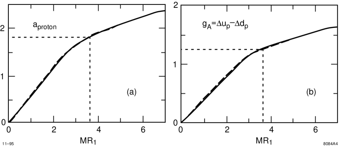
Figure 3: (a). The anomalous magnetic moment of the proton $a_{p}=F_{2}(0)$ as a function of its Dirac radius $M_{p}R_{1}$ in Compton units. (b). The axial vector coupling of the neutron to proton beta-decay as a function of $M_{p}R_{1}.$ In each figure, the broken line is computed from a wavefunction with power-law fall off and the solid curve is computed from a Gaussian wavefunction. The experimental values at the physical proton Dirac radius are indicated by the dotted line.

In Fig. 3(a) we show the functional relationship between the anomalous moment $a_{p}$ and its Dirac radius predicted by the three-quark light-cone model. The value of

$$R^{2}_{1}=-6\frac{dF_{1}(Q^{2})}{dQ^{2}}\Bigl{|}_{Q^{2}=0}$$ (45)

is varied by changing $\beta$ in the light-cone wavefunction while keeping the quark mass $m$ fixed. The prediction for the power-law wavefunction $\psi_{\rm Power}$ is given by the broken line; the continuous line represents $\psi_{\rm H.O.}$. Figure 3(a) shows that when one plots the dimensionless observable $a_{p}$ against the dimensionless observable $MR_{1}$ the prediction is essentially independent of the assumed power-law or Gaussian form of the three-quark light-cone wavefunction. Different values of $p>2$ also do not affect the functional dependence of $a_{p}(M_{p}R_{1})$ shown in Fig. 3(a). In this sense the predictions of the three-quark light-cone model relating the $Q^{2}\rightarrow 0$ observables are essentially model-independent. The only parameter controlling the relation between the dimensionless observables in the light-cone three-quark model is $m/M_{p}$ which is set to 0.28. For the physical proton radius $M_{p}R_{1}=3.63$ one obtains the empirical value for $a_{p}=1.79$ (indicated by the dotted lines in Fig. 3(a)).

The prediction for the anomalous moment $a$ can be written analytically as $a=\langle\gamma_{V}\rangle a^{\rm NR}$, where $a^{\rm NR}=2M_{p}/3m$ is the nonrelativistic ($R\rightarrow\infty$) value and $\gamma_{V}$ is given as $\!{}^{{\bf?}}$

$$\gamma_{V}(x_{i},k_{\perp i},m)=\frac{3m}{{\cal M}}\left[\frac{(1-x_{3}){\cal M}(m+x_{3}{\cal M})-\vec{k}_{\perp 3}^{2}/2}{(m+x_{3}{\cal M})^{2}+\vec{k}_{\perp 3}^{2}}\right]\;.$$ (46)

The expectation value $\langle\gamma_{V}\rangle$ is evaluated as

$$\langle\gamma_{V}\rangle=\frac{\int[d^{3}k]\gamma_{V}|\psi|^{2}}{\int[d^{3}k]|\psi|^{2}}\;.$$ (47)

Let us now take a closer look at the two limits $R\rightarrow\infty$ and $R\rightarrow 0$. In the nonrelativistic limit we let $\beta\rightarrow 0$ and keep the quark mass $m$ and the proton mass $M_{p}$ fixed. In this limit the proton radius $R_{1}\rightarrow\infty$ and $a_{p}\rightarrow 2M_{p}/3m=2.38$, since $\langle\gamma_{V}\rangle\rightarrow 1$. Thus the physical value of the anomalous magnetic moment at the empirical proton radius $M_{p}R_{1}=3.63$ is reduced by 25% from its nonrelativistic value due to relativistic recoil and nonzero $k_{\perp}$.

To obtain the ultra-relativistic limit we let $\beta\rightarrow\infty$ while keeping $m$ fixed. In this limit the proton becomes pointlike, $M_{p}R_{1}\rightarrow 0$, and the internal transverse momenta $k_{\perp}\rightarrow\infty$. The anomalous magnetic momentum of the proton goes linearly to zero as $a=0.43M_{p}R_{1}$ since $\langle\gamma_{V}\rangle\rightarrow 0$. Indeed, the Drell-Hearn-Gerasimov sum rule $\!{}^{{\bf?},{\bf?}}$ demands that the proton magnetic moment become equal to the Dirac moment at small radius. For a spin-$\frac{1}{2}$ system

$$a^{2}=\frac{M^{2}}{2\pi^{2}\alpha}\int_{s_{th}}^{\infty}\frac{ds}{s}\left[\sigma_{P}(s)-\sigma_{A}(s)\right]\;,$$ (48)

where $\sigma_{P(A)}$ is the total photo absorption cross section with parallel (anti-parallel) photon and target spins. If we take the point-like limit, such that the threshold for inelastic excitation becomes infinite while the mass of the system is kept finite, the integral over the photo absorption cross section vanishes and $a=0$.$\!{}^{{\bf?}}$ In contrast, the anomalous magnetic moment of the proton does not vanish in the nonrelativistic quark model as $R\rightarrow 0$. The nonrelativistic quark model does not reflect the fact that the magnetic moment of a baryon is derived from lepton scattering at nonzero momentum transfer, i.e., the calculation of a magnetic moment requires knowledge of the boosted wavefunction. The Melosh transformation is also essential for deriving the DHG sum rule and low-energy theorems of composite systems.$\!{}^{{\bf?}}$

A similar analysis can be performed for the axial-vector coupling measured in neutron decay. The coupling $g_{A}$ is given by the spin-conserving axial current $J_{A}^{+}$ matrix element

$$g_{A}(0)=\langle p,\uparrow|J^{+}_{A}|p,\uparrow\rangle\;.$$ (49)

The value for $g_{A}$ can be written as $g_{A}=\langle\gamma_{A}\rangle g_{A}^{\rm NR}$, with $g_{A}^{\rm NR}$ being the nonrelativistic value of $g_{A}$ and with $\gamma_{A}$ given by $\!{}^{{\bf?},{\bf?}}$

$$\gamma_{A}(x_{i},k_{\perp i},m)=\frac{(m+x_{3}{\cal M})^{2}-k_{\perp 3}^{2}}{(m+x_{3}{\cal M})^{2}+k_{\perp 3}^{2}}\;.$$ (50)

In Fig. 3(b) the axial-vector coupling is plotted against the proton radius $M_{p}R_{1}$. The same parameters and the same line representation as in Fig. 3(a) are used. The functional dependence of $g_{A}(M_{p}R_{1})$ is also found to be independent of the assumed wavefunction. At the physical proton radius $M_{p}R_{1}=3.63$, one predicts the value $g_{A}=1.25$ (indicated by the dotted lines in Fig. 3(b)), since $\langle\gamma_{A}\rangle=0.75$. The measured value is $g_{A}=1.2573\pm 0.0028$.$\!{}^{{\bf?}}$ This is a 25% reduction compared to the nonrelativistic SU(6) value $g_{A}=5/3,$ which is only valid for a proton with large radius $R_{1}\gg 1/M_{p}.$ The Melosh rotation generated by the internal transverse momentum $\!{}^{{\bf?}}$ spoils the usual identification of the $\gamma^{+}\gamma_{5}$ quark current matrix element with the total rest-frame spin projection $s_{z}$, thus resulting in a reduction of $g_{A}$.

Thus, given the empirical values for the proton’s anomalous moment $a_{p}$ and radius $M_{p}R_{1},$ its axial-vector coupling is automatically fixed at the value $g_{A}=1.25.$ This is an essentially model-independent prediction of the three-quark structure of the proton in QCD. The Melosh rotation of the light-cone wavefunction is crucial for reducing the value of the axial coupling from its nonrelativistic value 5/3 to its empirical value. The near equality of the ratios $g_{A}/g_{A}(R_{1}\rightarrow\infty)$ and $a_{p}/a_{p}(R_{1}\rightarrow\infty)$ as a function of the proton radius $R_{1}$ shows the wave-function independence of these quantities. We emphasize that at small proton radius the light-cone model predicts not only a vanishing anomalous moment but also $\lim_{R_{1}\rightarrow 0}g_{A}(M_{p}R_{1})=0$. One can understand this physically: in the zero radius limit the internal transverse momenta become infinite and the quark helicities become completely disoriented. This is in contradiction with chiral models, which suggest that for a zero radius composite baryon one should obtain the chiral symmetry result $g_{A}=1$.

The helicity measures $\Delta u$ and $\Delta d$ of the nucleon each experience the same reduction as does $g_{A}$ due to the Melosh effect. Indeed, the quantity $\Delta q$ is defined by the axial current matrix element

$$\Delta q=\langle p,\uparrow|\overline{q}\gamma^{+}\gamma_{5}q|p,\uparrow\rangle\;,$$ (51)

and the value for $\Delta q$ can be written analytically as $\Delta q=\langle\gamma_{A}\rangle\Delta q^{\rm NR}$, with $\Delta q^{\rm NR}$ being the nonrelativistic or naive value of $\Delta q$ and $\gamma_{A}$ given by Eq. (50).

The light-cone model also predicts that the quark helicity sum $\Delta\Sigma=\Delta u+\Delta d$ vanishes as the proton radius $R_{1}$ becomes small. Note that $\Delta\Sigma$ depends on the proton size, and it should not be identified as the vector sum of the rest-frame constituent spins. The rest-frame spin sum is not a Lorentz invariant for a composite system.$\!{}^{{\bf?}}$ Empirically, one can measure $\Delta q$ from the first moment of the leading-twist polarized structure function $g_{1}(x,Q).$ In the light-cone and parton model descriptions, $\Delta q=\int_{0}^{1}dx[q^{\uparrow}(x)-q^{\downarrow}(x)]$, where $q^{\uparrow}(x)$ and $q^{\downarrow}(x)$ can be interpreted as the probability for finding a quark or antiquark with longitudinal momentum fraction $x$ and polarization parallel or anti-parallel to the proton helicity in the proton’s infinite momentum frame.$\!{}^{{\bf?}}$ [In the infinite momentum frame there is no distinction between the quark helicity and its spin projection $s_{z}.$] Thus $\Delta q$ refers to the difference of helicities at fixed light-cone time or at infinite momentum; it cannot be identified with $q(s_{z}=+\frac{1}{2})-q(s_{z}=-\frac{1}{2}),$ the spin carried by each quark flavor in the proton rest frame in the equal-time formalism.

Thus the usual SU(6) values $\Delta u^{\rm NR}=4/3$ and $\Delta d^{\rm NR}=-1/3$ are only valid predictions for the proton at large $MR_{1}.$ At the physical radius the quark helicities are reduced by the same ratio 0.75 as is $g_{A}/g_{A}^{\rm NR}$ due to the Melosh rotation. Qualitative arguments for such a reduction have been given elsewhere.$\!{}^{{\bf?},{\bf?}}$ For $M_{p}R_{1}=3.63,$ the three-quark model predicts $\Delta u=1,$ $\Delta d=-1/4,$ and $\Delta\Sigma=\Delta u+\Delta d=0.75$. Although the gluon contribution $\Delta G=0$ in our model, the general sum rule $\!{}^{{\bf?}}$

$$\frac{1}{2}\Delta\Sigma+\Delta G+L_{z}=\frac{1}{2}$$ (52)

is still satisfied, since the Melosh transformation effectively contributes to $L_{z}$.

Suppose one adds polarized gluons to the three-quark light-cone model. Then the flavor-singlet quark-loop radiative corrections to the gluon propagator will give an anomalous contribution $\delta(\Delta q)=-\frac{\alpha_{s}}{2\pi}\Delta G$ to each light quark helicity.$\!{}^{{\bf?}}$ The predicted value of $g_{A}=\Delta u-\Delta d$ is of course unchanged. For illustration we shall choose $\frac{\alpha_{s}}{2\pi}\Delta G=0.15$. The gluon-enhanced quark model then gives values which agree well with the present experimental values.

In summary, one sees that relativistic effects are crucial for understanding the spin structure of nucleons. By plotting dimensionless observables against dimensionless observables, we obtain relations that are independent of the momentum-space form of the three-quark light-cone wavefunctions. For example, the value of $g_{A}\simeq 1.25$ is correctly predicted from the empirical value of the proton’s anomalous moment. For the physical proton radius $M_{p}R_{1}=3.63$, the inclusion of the Wigner-Melosh rotation due to the finite relative transverse momenta of the three quarks results in a $\sim 25\%$ reduction of the nonrelativistic predictions for the anomalous magnetic moment, the axial vector coupling, and the quark helicity content of the proton. At zero radius, the quark helicities become completely disoriented because of the large internal momenta, resulting in the vanishing of $g_{A}$ and the total quark helicity $\Delta\Sigma.$

8 Constructing Hadron Wavefunctions in Light-Cone Quantized QCD

Our ultimate goal is to actually calculate the light cone wavefunctions of the hadrons. In the next two sections, I will discuss possible methods in which one can obtain constraints and determine important properties of the wavefunctions, even in the absence of explicit solutions.

A remarkable feature of collinear QCD is that although the theory is effectively one-space and one-time, one still retains the two physical degrees of freedom from the transversely-polarized gluons. Thus the spectrum of collinear QCD contains gluonium states, as well as gluonic quanta in the higher Fock states of the mesons and baryons eigenstates of the theory. We have also seen that some of the features of the structure functions of hadrons in collinear QCD match well to the phenomenological features of QCD[3+1] such as the helicity retention of the leading constituents at large $x\to 1$ in the polarized structure functions.

Recently Antonuccio, Pinsky and I have investigated the possibility that one may be able to construct useful models of the light-cone wavefunctions of QCD[3+1] by extension of the collinear QCD solutions. We have been considering two methods:

(1) Minimal Subtraction. Let us ignore the complications of spin and write the solution to the $n$-quark/antiquark light-cone wavefunction of a hadron in the collinear theory in the form

$$\Psi_{n}\left[\frac{m^{2}_{i}+g^{2}A^{2}_{\perp}}{x_{i}}\,,\,\overrightarrow{\!\!A}_{\perp}\right]$$

where the functional dependence of the operator $\Psi_{n}$ in the field variable $\overrightarrow{\!\!A}_{\perp}$ connects Fock states of different gluon number. The natural generalization of this dependence to the transverse space dependence is

$$\Psi_{n}\rightarrow\Psi_{n}\left[\frac{m^{2}_{i}+(\overrightarrow{\!\!k}_{\perp}-g\overrightarrow{\!\!A}_{\perp})^{2}}{x_{i}}\,,\,\left(\overrightarrow{\!\!k}_{\perp}-g\overrightarrow{\!\!A}_{\perp}\right)\right]$$

It is interesting to note that the mechanical light-cone kinetic energy

$$\frac{m^{2}_{i}+(\overrightarrow{\!\!k}_{\perp}-g\overrightarrow{\!\!A}_{\perp})^{2}}{x_{i}}\,$$

is the essential variable which controls the dynamics of gauge theory. This is in agreement with the fact that in laser physics the effective mass of an electron in an intense laser beam is $m_{\rm effective}^{2}=m_{e}^{2}+e^{2}A^{2}.$ The laser analog also suggest that a classical approximation to the gauge field may be useful when the particle number is high. This could be appropriate when analyzing the physics of small $x$.

(2) The Light-Cone Lippmann-Schwinger Equation. In principle, we can also construct the wavefunctions of QCD(3+1) starting with collinear QCD(1+1) solutions by systematic perturbation theory in $\Delta H$, where $\Delta H$ contains the terms linear and quadratic in the transverse momenta $\overrightarrow{\!\!k}_{\perp i}$ which are neglected in the Hamilton $H_{0}$ of collinear QCD. We can write the exact eigensolution of the full Hamiltonian as

$$\psi_{(3+1)}=\psi_{(1+1)}+\frac{1}{M^{2}-H+i\epsilon}\,\Delta H\,\psi_{(1+1)}\ ,$$

where

$$\frac{1}{M^{2}-H+i\epsilon}={\frac{1}{M^{2}-H_{0}+i\epsilon}}+{\frac{1}{M^{2}-H+i\epsilon}}\Delta H{\frac{1}{M^{2}-H_{0}+i\epsilon}}$$

can be represented as the continued iteration of the Lippmann Schwinger resolvant. Note that the matrix $(M^{2}-H_{0})^{-1}$ is known to any desired precision from the DLCQ solution of collinear QCD.

In each of these methods, the resulting wavefunction can be considered as approximate solution to 3+1 QCD hadron wavefunctions which could be subsequently improved by variational or other methods.

9 Determining the Far Off-Shell Behavior of Hadron LC Wavefunctions

In many cases of physical interest we are specifically interested in the behavior of the LC wavefunctions in the far-off-shell domain where ${\cal M}^{2}_{n}$ exceeds the global cutoff. This occurs for large parton momenta, $k^{2}_{\perp}\rightarrow\infty$, $x_{i}\rightarrow 1$ and for massive quanti-antiquark fluctuations. In fact, in such domains, we can construct the wavefunction perturbatively and obtain rigorous QCD predictions.

The basic method is as follows.$\!{}^{{\bf?}}$ Suppose we can solve

$$H_{LC}(\mu)\,\left|\,{\psi^{(\mu)}}\right\rangle=M^{2}\,\left|\,{\psi^{(\mu)}}\right\rangle$$ (53)

in the soft-domain with ${\cal M}^{2}_{n}<\mu^{2}$, where $\mu^{2}$ is of the order of a few GeV². Then

$$\,\left|\,{\psi^{(\mu)}}\right\rangle=\sum_{n}\,\left|\,{n}\right\rangle\left\langle{n\,|\,\psi}\right\rangle\,\theta(\mu^{2}-M^{2}_{n})\equiv P^{(\mu)}\,\left|\,{\psi}\right\rangle\ .$$ (54)

We can also define the complement projection operator $Q^{(\mu)}$ with $P^{(\mu)}+Q^{(\mu)}=1$. The full solution satisfies $H\,\left|\,{\psi}\right\rangle=M^{2}\,\left|\,{\psi}\right\rangle$ or

$$PHP\,\left|\,{\psi}\right\rangle+PHQ\,\left|\,{\psi}\right\rangle = M^{2}P\,\left|\,{\psi}\right\rangle$$

$$QHP\,\left|\,{\psi}\right\rangle+QHQ\,\left|\,{\psi}\right\rangle = M^{2}Q\,\left|\,{\psi}\right\rangle\ .$$ (55)

Therefore

$$\,\left|\,{\psi}\right\rangle=\,\left|\,{\psi^{(\mu)}}\right\rangle+\frac{1}{M^{2}-QHQ}\ QH_{\pm}\,\left|\,{\psi^{(\mu)}}\right\rangle$$ (56)

where only high mass $({\cal M}^{2}_{n}>\mu^{2})$ perturbatively calculable intermediate states appear. An example is the behavior of the valence wavefunction at large internal transverse momentum. One finds at large $\vec{k}_{\perp}=\vec{q}_{\perp}$

$$\psi(x,q_{\perp}) = \frac{1}{m^{2}-\frac{\vec{q}^{2}_{\perp}+m^{2}}{x(1-x)}}\int^{1}_{0}dy\int d^{2}\ell_{\perp}\,V(x,q_{\perp};y,\ell_{\perp})\,\psi^{(\mu)}(y,\ell_{\perp})$$ (57)

$$\cong -\frac{x(1-x)}{\vec{q}^{2}_{\perp}}\ \alpha_{s}(\vec{q}^{2}_{\perp})\int^{1}_{0}dy\,V_{1g}(x,y)\,\psi(y,q^{2}_{\perp})$$

where

$$\phi(y,Q^{2})=\int^{Q^{2}}\frac{d^{3}\ell_{\perp}}{16\pi^{3}}\ \psi_{(2)}(y,\ell_{\perp})$$ (58)

is the meson distribution amplitude, which takes the role of the wavefunction “at-the-origin” in analogous nonrelativistic calculations. The simple $\alpha_{s}(q^{2}_{\perp})/\vec{q}^{2}_{\perp}$ fall-off of the valence wavefunction is the key input to the derivation of dimensional counting rules for form factors and other exclusive processes in QCD.$\!{}^{{\bf?}}$ One can also derive the evolution equation for

$$\frac{\partial\phi(y,Q^{2})}{\partial\log Q^{2}}$$ (59)

from this result and the simple properties of the one-gluon exchange kernel.

10 Structure Functions at the End-Point

The $x\rightarrow 1$ behavior of quark and gluon wavefunctions is controlled by far-off-shell configuration and thus can be analyzed perturbatively. The dominant contributions come from the lowest Fock states which contain the partons. For example the quark distribution in the nucleon can be computed from two iterations of the gluon exchange kernel which transfers the light-cone momentum to the struck quark from the two spectators which are required to stop. The result is a nominal power-law fall-off at $x\rightarrow 1$: $q_{\uparrow}(x)\sim(1-x)^{3}$ for quarks with helicity aligned with the proton and $q_{\downarrow}\sim(1-x)^{5}$ for quarks anti-aligned. Similarly the $\,\left|\,{qqqg}\right\rangle$ Fock state yields $g_{\uparrow}(x)\sim(1-x)^{4}$ for gluons with helicity aligned and $g_{\downarrow}\sim(1-x)^{6}$ for gluons helicity anti-aligned. Thus the partons with $x\rightarrow 1$ tend to have the same sign helicity as the bound state.$\!{}^{{\bf?}}$

In the absence of full solutions to the light-cone wavefunctions, one can construct a simple phenomenology of the polarized and anti-polarized structure functions by imposing a smooth connection between the perturbative QCD constraints at $x\rightarrow 1$, and Regge behavior at $x\rightarrow 0$, and the momentum and Bjorken sum rules. A complete discussion can be found in the literature.$\!{}^{{\bf?}}$ Recently Leader et al. have shown that this parametrization agrees remarkably well with the available data from SLAC and CERN.$\!{}^{{\bf?}}$ Figure 4 shows the nominal form of the helicity distributions $\Delta q(x)=q_{\uparrow}(x)-q_{\downarrow}(x)$, for the valance quarks and gluons in the proton.

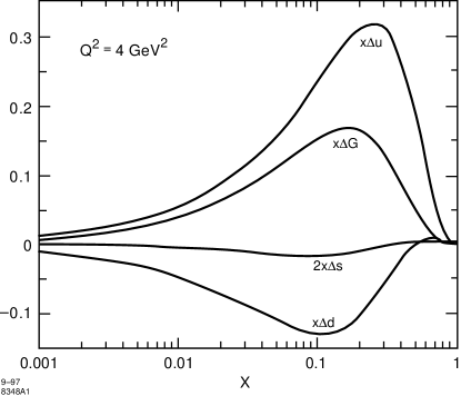
Figure 4: Model form for the polarized quark and gluon distributions of the proton satisfying empirical constraints and the perturbative QCD and Regge input conditions.$\!{}^{{\bf?}}$ From Leader et al.$\!{}^{{\bf?}}$

11 Intrinsic Hardness

The light-cone wavefunctions contain high fluctuations of arbitrary mass; i.e. nonzero probabilities for massive pairs, massive sea quarks, etc. These fluctuations are of two types: extrinsic $qg$, $gg$ or $q\overline{q}$ high mass pairs which are associated with the substructure of the constituents and are contained in ordinary DGLAP evolution; and intrinsic functions which are due to the physics of the bound state wavefunction itself. For example intrinsic sea quark pairs $Q\overline{Q}$ arise from diagrams which are interconnected to the valence quarks of the bound state hadron and thus depend on the valence quark correlations. It is easy to see that the leading perturbative contribution to intrinsic pairs falls as

$$\psi\sim\frac{\alpha_{s}^{2+\Gamma}({\cal M}^{2})}{{\cal M}^{2}}$$ (60)

where ${\cal M}$ is the pair mass and $T$ is the leading anomalous dimension associated with the valence wavefunction. The probability of any configurations with ${\cal M}^{2}>{\cal M}^{2}_{0}$ is then

$$P({\cal M}^{2}>{\cal M}^{2}_{0})\sim\frac{\alpha_{s}^{4+2\Gamma}}{{\cal M}^{2}_{0}}\ ,$$ (61)

which implies a remarkably slow fall-off for large off-shell fluctuations. The result is universal for any intrinsic parton pair

$$\frac{{\cal M}^{2}+P^{2}_{\perp}}{x_{1}+x_{2}}=\frac{m^{2}_{1}+\vec{k}^{2}_{\perp i}}{x_{1}}+\frac{m^{2}_{2}+\vec{k}^{2}_{\perp 2}}{x_{2}}$$ (62)

with

$$\vec{k}_{\perp 1}=x_{1}\vec{P}_{\perp}+\vec{k}_{\perp}\qquad\vec{k}_{\perp 2}=x_{2}\vec{P}_{\perp}-\vec{k}_{\perp}\ ;$$ (63)

i.e. for large relative $k_{\perp}$ and/or large quark mass. Hoyer and I $\!{}^{{\bf?}}$ call this “intrinsic hardness.” In the case of intrinsic charm or bottom pairs in the nucleon, the LC wavefunction is maximized when ${\cal M}^{2}_{n}$ is minimized; i.e. for

$$x_{\perp i}=\frac{m_{\perp i}}{\Sigma m_{\perp i}}$$ (64)

where $m_{\perp}=\sqrt{m^{2}+\vec{k}^{2}_{\perp}}$. Thus the maximal intrinsic charm-bottom configurations occur at equal rapidity; i.e. where the heavy partons have highest momentum fractions. This is in contrast to the usual extrinsic sea quark which are subconstituents of the gluons and have low $x$. The extrinsic quarks evolve rapidly with a probability increasing as power of $\log\,Q^{2}/{\cal M}^{2}$.

It is thus important to distinguish two types of quark and gluon contributions to the nucleon sea measured in deep inelastic lepton-nucleon scattering: “extrinsic” and “intrinsic”. $\!{}^{{\bf?}}$ The extrinsic sea quarks and gluons are created as part of the lepton-scattering interaction and thus exist over a very short time $\Delta\tau\sim 1/Q$. These factorizable contributions can be systematically derived from the QCD hard bremsstrahlung and pair-production (gluon-splitting) subprocesses characteristic of leading twist perturbative QCD evolution. In contrast, the intrinsic sea quarks and gluons are multi-connected to the valence quarks and exist over a relatively long lifetime within the nucleon bound state. Thus the intrinsic $q\overline{q}$ pairs can arrange themselves together with the valence quarks of the target nucleon into the most energetically-favored meson-baryon fluctuations.

Another interesting distinction between extrinsic and intrinsic sea quarks is that due to nonperturbative effects, the intrinsic contributions are generally not symmetric for sea quark and anti-quarks. For example, in the muonium atom $(\mu^{+}e^{-})$ an intrinsic $\tau^{+}\tau^{-}$ pair would be asymmetric since the $\tau^{+}$ tends to be attracted to the electron and the $\tau^{-}$ tends to be attracted to the opposite-sign muon. Thus the $\tau^{-}$ would be expected to have a higher $\left\langle{x}\right\rangle$ than the $\tau^{+}$. It is also possible to consider the nucleon wavefunction at low resolution as a fluctuating system coupling to intermediate hadronic Fock states such as non-interacting meson-baryon pairs. The most important fluctuations are most likely to be those closest to the energy shell and thus have minimal invariant mass. For example, the coupling of a proton to a virtual $K^{+}\Lambda$ pair provides a specific source of intrinsic strange quarks and antiquarks in the proton. Since the $s$ and $\overline{s}$ quarks appear in different configurations in the lowest-lying hadronic pair states, their helicity and momentum distributions are distinct. Ma and I $\!{}^{{\bf?}}$ have used an intermediate meson-baryon fluctuation model to model the possible $s$ versus $\overline{s}$ and $c$ versus $\overline{c}$ asymmetries of the intrinsic distributions of the nucleon. We utilize a boost-invariant light-cone Fock state description of the hadron wavefunction which emphasizes multi-parton configurations of minimal invariant mass. We find that such fluctuations predict a striking sea quark/antiquark asymmetry in the corresponding momentum and helicity distributions in the nucleon structure functions. In particular, the strange and anti-strange distributions in the nucleon generally have completely different momentum and spin characteristics. The helicity structure of the intrinsic $s\overline{s}$ is strongly asymmetric: the $s$ quark from a $\Lambda(uds)\,K(u\overline{s})$ is aligned with the $\Lambda$ helicity and (because of parity) is 100% anti-aligned with the nucleon spin. On the other hand, the $\overline{s}$ from the pseudoscalar kaon is unaligned. Ma and I have shown that this picture of quark and antiquark asymmetry in the momentum and helicity distributions of the nucleon sea quarks has support from a number of experimental observations, and we have suggested processes to test and measure this quark and antiquark asymmetry in the nucleon sea.

11.1 Phenomenological Consequences of Intrinsic Charm and Bottom

Microscopically, the intrinsic heavy-quark Fock component in the $\pi^{-}$ wavefunction, $|\overline{u}dQ\overline{Q}\rangle$, is generated by virtual interactions such as $gg\rightarrow Q\overline{Q}$ where the gluons couple to two or more projectile valence quarks. The probability for $Q\overline{Q}$ fluctuations to exist in a light hadron thus scales as $\alpha_{s}^{2}(m_{Q}^{2})/m_{Q}^{2}$ relative to leading-twist production.$\!{}^{{\bf?}}$ This contribution is therefore higher twist, and power-law suppressed compared to sea quark contributions generated by gluon splitting. When the projectile scatters in the target, the coherence of the Fock components is broken and its fluctuations can hadronize, forming new hadronic systems from the fluctuations.$\!{}^{{\bf?}}$ For example, intrinsic $c\overline{c}$ fluctuations can be liberated provided the system is probed during the characteristic time $\Delta t=2p_{\rm lab}/M^{2}_{c\overline{c}}$ that such fluctuations exist. For soft interactions at momentum scale $\mu$, the intrinsic heavy quark cross section is suppressed by an additional resolving factor $\propto\mu^{2}/m^{2}_{Q}$.$\!{}^{{\bf?}}$ The nuclear dependence arising from the manifestation of intrinsic charm is expected to be $\sigma_{A}\approx\sigma_{N}A^{2/3}$, characteristic of soft interactions.

In general, the dominant Fock state configurations are not far off shell and thus have minimal invariant mass ${\cal M}^{2}=\sum_{i}m_{\perp}/x_{i}$ where $m_{\perp}$ is the transverse mass of the $i^{\rm th}$ particle in the configuration. Intrinsic $Q\overline{Q}$ Fock components with minimum invariant mass correspond to configurations with equal-rapidity constituents. Thus, unlike sea quarks generated from a single parton, intrinsic heavy quarks tend to carry a larger fraction of the parent momentum than do the light quarks.$\!{}^{{\bf?}}$ In fact, if the intrinsic $Q\overline{Q}$ pair coalesces into a quarkonium state, the momentum of the two heavy quarks is combined so that the quarkonium state will carry a significant fraction of the projectile momentum.

There is substantial evidence for the existence of intrinsic $c\overline{c}$ fluctuations in the wavefunctions of light hadrons. For example, the charm structure function of the proton measured by EMC is significantly larger than that predicted by photon-gluon fusion at large $x_{Bj}$.$\!{}^{{\bf?}}$ Leading charm production in $\pi N$ and hyperon-$N$ collisions also requires a charm source beyond leading twist.$\!{}^{{\bf?},{\bf?}}$ The NA3 experiment has also shown that the single $J/\psi$ cross section at large $x_{F}$ is greater than expected from $gg$ and $q\overline{q}$ production.$\!{}^{{\bf?}}$ The nuclear dependence of this forward component is diffractive-like, as expected from the BHMT mechanism. In addition, intrinsic charm may account for the anomalous longitudinal polarization of the $J/\psi$ at large $x_{F}$ seen in $\pi N\rightarrow J/\psi X$ interactions.$\!{}^{{\bf?}}$ Further theoretical work is needed to establish that the data on direct $J/\psi$ and $\chi_{1}$ production can be described using the higher-twist intrinsic charm mechanism.$\!{}^{{\bf?}}$

A recent analysis by Harris, Smith and Vogt $\!{}^{{\bf?}}$ of the excessively large charm structure function of the proton at large $x$ as measured by the EMC collaboration at CERN yields an estimate that the probability $P_{c\overline{c}}$ that the proton contains intrinsic charm Fock states is of the order of $0.6\%\pm 0.3\%.$ In the case of intrinsic bottom, perturbative QCD scaling predicts

$$P_{b\overline{b}}=P_{c\overline{c}}\frac{m^{2}_{\psi}}{m^{2}_{\Upsilon}}\frac{\alpha^{4}_{s}(m_{b})}{\alpha^{4}_{s}(m_{c})}\;,$$ (65)

more than an order of magnitude smaller. We can speculate that if super-partners of the quarks or gluons exist they must also appear in higher Fock states of the proton, such as $|uud~{}{\rm gluino}~{}{\rm gluino}\rangle$. At sufficiently high energies, the diffractive excitation of the proton will produce these intrinsic quarks and gluinos in the proton fragmentation region. Such supersymmetric particles can bind with the valence quarks to produce highly unusual color-singlet hybrid supersymmetric states such as $|uud~{}{\rm gluino}\rangle$ at high $x_{F}.$ The probability that the proton contains intrinsic gluinos or squarks scales with the appropriate color factor and scales inversely with the heavy particle mass squared relative to the intrinsic charm and bottom probabilities. This probability is directly reflected in the production rate when the hadron is probed at a hard scale $Q$ which is large compared to the virtual mass ${\cal M}$ of the Fock state. At low virtualities, the rate is suppressed by an extra resolution factor of $Q^{2}/{\cal M}^{2}.$ The forward proton fragmentation regime is a challenge to instrument at HERA, but it may be feasible to tag special channels involving neutral hadrons or muons. In the case of the gas jet fixed-target $ep$ collisions such as at HERMES, the target fragments emerge at low velocity and large backward angles, and thus may be accessible to precise measurement.

Double Quarkonium Hadroproduction It is quite rare for two charmonium states to be produced in the same hadronic collision. However, the NA3 collaboration has measured a double $J/\psi$ production rate significantly above background in multi-muon events with $\pi^{-}$ beams at laboratory momentum 150 and 280 GeV/c and a 400 GeV/c proton beam. $\!{}^{{\bf?}}$ The relative double to single rate, $\sigma_{\psi\psi}/\sigma_{\psi}$, is $(3\pm 1)\times 10^{-4}$ for pion-induced production, where $\sigma_{\psi}$ is the integrated single $\psi$ production cross section. A particularly surprising feature of the NA3 $\pi^{-}N\rightarrow\psi\psi X$ events is that the laboratory fraction of the projectile momentum carried by the $\psi\psi$ pair is always very large, $x_{\psi\psi}\geq 0.6$ at 150 GeV/c and $x_{\psi\psi}\geq 0.4$ at 280 GeV/c. In some events, nearly all of the projectile momentum is carried by the $\psi\psi$ system! In contrast, perturbative $gg$ and $q\overline{q}$ fusion processes are expected to produce central $\psi\psi$ pairs, centered around the mean value, $\langle x_{\psi\psi}\rangle\approx$ 0.4–0.5, in the laboratory. The predicted $\psi\psi$ pair distributions from the intrinsic charm model provide a natural explanation of the strong forward production of double $J/\psi$ hadroproduction, and thus gives strong phenomenological support for the presence of intrinsic heavy quark states in hadrons.

It is clearly important for the double $J/\psi$ measurements to be repeated with higher statistics and at higher energies. The same intrinsic Fock states will also lead to the production of multi-charmed baryons in the proton fragmentation region. The intrinsic heavy quark model can also be used to predict the features of heavier quarkonium hadroproduction, such as $\Upsilon\Upsilon$, $\Upsilon\psi$, and $(c\overline{b})$ $(\overline{c}b)$ pairs. Predictions for these events have been given by Ramona Vogt and myself.

Leading-Particle Effect in Open Charm Production According to PQCD factorization, the fragmentation of a heavy quark jet is independent of the production process. However, there are strong correlations between the quantum numbers of $D$ mesons and the charge of the incident pion beam in $\pi N\rightarrow DX$ reactions. This effect can be explained as being due to the coalescence of the produced intrinsic charm quark with co-moving valence quarks. The same higher-twist recombination effect can also account for the suppression of $J/\psi$ and $\Upsilon$ production in nuclear collisions in regions of phase space with high particle density.$\!{}^{{\bf?}}$

It is of particular interest to examine the fragmentation of the proton when the electron strikes a light quark and the interacting Fock component is the $|uudc\overline{c}\rangle$ or $|uudb\overline{b}\rangle$ state. These Fock components correspond to intrinsic charm or intrinsic bottom quarks in the proton wavefunction. Since the heavy quarks in the proton bound state have roughly the same rapidity as the proton itself, the intrinsic heavy quarks will appear in the proton fragmentation region. One expects heavy quarkonium and also heavy hadrons to be formed from the coalescence of the heavy quark with the valence $u$ and $d$ quarks, since they have nearly the same rapidity.

12 Intrinsic Charm and the $J/\psi\to\rho\pi$ problem

One of the most dramatic problems confronting the standard picture of quarkonium decays is the $J/\psi\to\rho\pi$ puzzle.$\!{}^{{\bf?}}$ This decay occurs with a branching ratio of $(1.28\pm 0.10)\%$,$\!{}^{{\bf?}}$ and it is the largest two-body hadronic branching ratio of the $J/\psi$. The $J/\psi$ is assumed to be a $\overline{c}c$ bound state pair in the $\Psi(1S)$ state. One then expects the $\psi^{\prime}=\Psi(2S)$ to decay to $\rho\pi$ with a comparable branching ratio, scaled by a factor $\sim 0.15$, due to the ratio of the $\Psi(2S)$ to $\Psi(1S)$ wavefunctions squared at the origin. In fact, $B(\psi^{\prime}\to\rho\pi)<3.6\times 10^{-5}$ ,$\!{}^{{\bf?}}$ more than a factor of 50 below the expected rate. Most of the branching ratios for exclusive hadronic channels allowed in both $J/\psi$ and $\psi^{\prime}$ decays indeed scale with their lepton pair branching ratios, as would be expected from decay amplitudes controlled by the quarkonium wavefunction near the origin,$\!{}^{{\bf?},{\bf?}}$

$${B(\psi^{\prime}\to h)\over B(J/\psi\to h)}\simeq{B(\psi^{\prime}\to e^{+}e^{-})\over B(J/\psi\to e^{+}e^{-})}=0.147\pm 0.023\quad$$ (66)

where $h$ denotes a given hadronic channel. The $J/\psi\to\rho\pi$ and $J/\psi\to KK^{*}$ decays also conflict dramatically with perturbative QCD hadron helicity conservation: all such pseudoscalar/vector two-body hadronic final states are forbidden at leading twist if helicity is conserved at each vertex.$\!{}^{{\bf?},{\bf?}}$

Marek Karliner and I $\!{}^{{\bf?}}$ have recently shown that such anomalously large decay rates for the $J/\psi$ and their suppression for $\psi^{\prime}(2S)$ follow naturally from the existence of intrinsic charm $\,\left|\,{\overline{q}q\,\overline{c}c}\right\rangle$ Fock components of the light vector mesons. For example, consider the light-cone Fock representation of the $\rho$: $\rho^{+}=\Psi^{\rho}_{u\overline{d}}\,\,\left|\,{u\overline{d}}\right\rangle\,+\,\Psi^{\rho}_{u\overline{d}\,\overline{c}c}\,\,\left|\,{u\overline{d}\,\overline{c}c}\right\rangle\,+\,\cdots\ \ .$ The $\Psi^{\rho}_{u\overline{d}\overline{c}c}$ wavefunction will be maximized at minimal invariant mass; i.e. at equal rapidity for the constituents and in the spin configuration where the $u\overline{d}$ are in a pseudoscalar state, thus minimizing the QCD spin-spin interaction. The $\overline{c}c$ in the $\,\left|\,{u\overline{d}\,\overline{c}c}\right\rangle$ Fock state carries the spin projection of the $\rho.$ We also expect the wavefunction of the $\overline{c}c$ quarks to be in an $S$-wave configuration with no nodes in its radial dependence, in order to minimize the kinetic energy of the charm quarks and thus also minimize the total invariant mass.

The presence of the $\,\left|\,{u\overline{d}\,\overline{c}c}\right\rangle$ Fock state in the $\rho$ will allow the $J/\psi\to\rho\pi$ decay to occur simply through rearrangement of the incoming and outgoing quark lines; in fact, the $\,\left|\,{u\overline{d}\,\overline{c}c}\right\rangle$ Fock state wavefunction has a good overlap with the radial and spin $\,\left|\,{\overline{c}c}\right\rangle$ and $\,\left|\,{u\overline{d}}\right\rangle$ wavefunctions of the $J/\psi$ and pion. Moreover, there is no conflict with hadron helicity conservation, since the $\overline{c}c$ pair in the $\rho$ is in the $1^{-}$ state. On the other hand, the overlap with the $\psi^{\prime}$ will be suppressed, since the radial wavefunction of the $n=2$ quarkonium state is orthogonal to the node-less $\overline{c}c$ in the $\,\left|\,{u\overline{d}\,\overline{c}c}\right\rangle$ state of the $\rho$. This simple argument provides a compelling explanation of the absence of $\psi^{\prime}\to\rho\pi$ and other vector pseudoscalar-scalar states.

13 Light-Cone Wavefunction Description of the Spin Anomaly in Deep Inelastic Polarized Structure Functions

One of the most interesting distinguishing characteristics between extrinsic and intrinsic heavy quarks is their contributions to the Ellis-Jaffe sum rule $\int^{1}_{0}dx\,g_{1}(x,Q)$ for polarized deep inelastic scattering cross sections. The extrinsic contributions to structure functions can be identified with photon-gluon fusion processes since they derive from $Q\overline{Q}$ constituents of the gluon. However, one obtains zero contribution to the Ellis-Jaffe sum rule from $\gamma^{*}g\rightarrow q\overline{q}$ at tree level if the gluon is on-shell $k^{2}=0$. This follows from the DHG sum rule: the tree graph contribution to $\!{}^{{\bf?}}$

$$\int^{\infty}_{\nu_{th}}\frac{d{\nu}}{\nu}\,\Delta\sigma(ab\rightarrow cd)$$ (67)

vanishes for any two-to-two polarized cross sections if $a$ is an on-shell gauge particle. Thus the anomaly contribution $-\frac{\alpha_{s}}{2\pi}\,\Delta G$ to the Ellis-Jaffe sum rule arises from off-shell gluons with $|k^{2}|\buildrel>\over{{}_{\sim}}4m^{2}_{Q}$.$\!{}^{{\bf?}}$ The final state which contributes physically to such configurations consists of $Q$ and $\overline{Q}$ jets recoiling against the scattered lepton plus a third jet scattering at $p_{T}>m_{Q}$, corresponding to a quark (or gluon) which emitted the off-shell gluon. The intrinsic contributions, on the other hand, consist of one high $p_{T}$ heavy quark jet recoiling against the lepton. Also, as noted above, the $\Delta Q(x)$ and $\Delta\overline{Q}(x)$ in general are different helicity distributions.$\!{}^{{\bf?}}$

14 Direct Measurement of the Light-cone Valence Wavefunction.

Diffractive multi-jet production in heavy nuclei provides a novel way to measure the shape of the LC Fock state wavefunctions. For example, consider the reaction $\!{}^{{\bf?},{\bf?}}$

$$\pi A\rightarrow{\rm Jet}_{1}+{\rm Jet}_{2}+A^{\prime}$$ (68)

at high energy where the nucleus $A^{\prime}$ is left intact in its ground state. The transverse momenta of the jets have to balance so that $\vec{k}_{\perp i}+\vec{k}_{\perp 2}=\vec{q}_{\perp}<{\cal R}^{-1}_{A}\ ,$ and the light-cone longitudinal momentum fractions have to add to $x_{1}+x_{2}\sim 1$ so that $\Delta p_{L}<{\cal R}^{-1}_{A}$. The process can then occur coherently in the nucleus. Because of color transparency; i.e. the cancellation of color interactions in a small-size color-singlet hadron, the valence wavefunction of the pion with small impact separation, will penetrate the nucleus with minimal interactions, diffracting into jet pairs.$\!{}^{{\bf?}}$ The $x_{1}=x$, $x_{2}=1-x$ dependence of the di-jet distributions will thus reflect the shape of the pion distribution amplitude; the $\vec{k}_{\perp 1}-\vec{k}_{\perp 2}$ relative transverse momenta of the jets also gives key information on the underlying shape of the valence pion wavefunction. The QCD analysis can be confirmed by the observation that the diffractive nuclear amplitude extrapolated to $t=0$ is linear in nuclear number $A$, as predicted by QCD color transparency. The integrated diffractive rate should scale as $A^{2}/{\cal R}^{2}_{A}\sim A^{4/3}$. A diffractive experiment of this type is now in progress at Fermilab using 500 GeV incident pions on nuclear targets.$\!{}^{{\bf?}}$

Data from CLEO for the $\gamma\gamma^{*}\rightarrow\pi^{0}$ transition form factor favor a form for the pion distribution amplitude close to the asymptotic solution $\!{}^{{\bf?}}$ $\phi^{asympt}_{\pi}(x)=\sqrt{3}f_{\pi}x(1-x)$ to the perturbative QCD evolution equation.$\!{}^{{\bf?},{\bf?},{\bf?}}$ It will be interesting to see if the diffractive pion to di-jet experiment also favors the asymptotic form.

It would also be interesting to study diffractive tri-jet production using proton beams $pA\rightarrow{\rm Jet}_{1}+{\rm Jet}_{2}+{\rm Jet}_{3}+A^{\prime}$ to determine the fundamental shape of the 3-quark structure of the valence light-cone wavefunction of the nucleon at small transverse separation. Conversely, one can use incident real and virtual photons: $\gamma^{*}A\rightarrow{\rm Jet}_{1}+{\rm Jet}_{2}+A^{\prime}$ to confirm the shape of the calculable light-cone wavefunction for transversely-polarized and longitudinally-polarized virtual photons. Such experiments will open up a remarkable, direct window on the amplitude structure of hadrons at short distances.

15 Other Applications of Light-Cone Quantization to Hadron Phenomenology

The light-cone formalism provides the theoretical framework which allows for a hadron to exist in various Fock configurations. For example, quarkonium states not only have valence $Q\overline{Q}$ components but they also contain $Q\overline{Q}g$ and $Q\overline{Q}gg$ states in which the quark pair is in a color-octet configuration. Similarly, nuclear LC wave functions contain components in which the quarks are not in color-singlet nucleon sub-clusters. In some processes, such as large momentum transfer exclusive reactions, only the valence color-singlet Fock state of the scattering hadrons with small inter-quark impact separation $b_{\perp}={\cal O}(1/Q)$ can couple to the hard scattering amplitude. In reactions in which large numbers of particles are produced, the higher Fock components of the LC wavefunction will be emphasized. The higher particle number Fock states of a hadron containing heavy quarks can be diffractively excited, leading to heavy hadron production in the high momentum fragmentation region of the projectile. In some cases the projectile’s valence quarks can coalesce with quarks produced in the collision, producing unusual leading-particle correlations. Thus the multi-particle nature of the LC wavefunction can manifest itself in a number of novel ways. For example:

Regge behavior. The light-cone wavefunctions $\psi_{n/H}$ of a hadron are not independent of each other, but rather are coupled via the equations of motion. Recently Antonuccio, Dalley and I $\!{}^{{\bf?}}$ have used the constraint of finite “mechanical” kinetic energy to derive“ladder relations” which interrelate the light-cone wavefunctions of states differing by 1 or 2 gluons. We then use these relations to derive the Regge behavior of both the polarized and unpolarized structure functions at $x\rightarrow 0$, extending Mueller’s derivation of the BFKL hard QCD pomeron from the properties of heavy quarkonium light-cone wavefunctions at large $N_{C}$ QCD.$\!{}^{{\bf?}}$

Analysis of diffractive vector meson photoproduction. The light-cone Fock wavefunction representation of hadronic amplitudes allows a simple eikonal analysis of diffractive high energy processes, such as $\gamma^{*}(Q^{2})p\to\rho p$, in terms of the virtual photon and the vector meson Fock state light-cone wavefunctions convoluted with the $gp\to gp$ near-forward matrix element $\!{}^{{\bf?}}$ See Fig. 1h. One can easily show that only small transverse size $b_{\perp}\sim 1/Q$ of the vector meson wavefunction is involved. The hadronic interactions are minimal, and thus the $\gamma^{*}(Q^{2})N\to\rho N$ reaction can occur coherently throughout a nuclear target in reactions such as without absorption or shadowing. The $\gamma^{*}A\to\phi A$ process thus provides a natural framework for testing QCD color transparency.$\!{}^{{\bf?}}$

Structure functions at large $x_{bj}$. The behavior of structure functions where one quark has the entire momentum requires the knowledge of LC wavefunctions with $x\rightarrow 1$ for the struck quark and $x\rightarrow 0$ for the spectators. As mentioned in Section 2, this is a highly off-shell configuration, and thus one can rigorously derive quark-counting and helicity-retention rules for the power-law behavior of the polarized and unpolarized quark and gluon distributions in the $x\rightarrow 1$ endpoint domain. Evolution of structure functions is minimal in this domain because the struck quark is highly virtual as $x\rightarrow 1$; i.e. the starting point $Q^{2}_{0}$ for evolution cannot be held fixed, but must be larger than a scale of order $(m^{2}+k^{2}_{\perp})/(1-x)$.$\!{}^{{\bf?}}$

Color Transparency QCD predicts that the Fock components of a hadron with a small color dipole moment can pass through nuclear matter without interactions.$\!{}^{{\bf?},{\bf?}}$ Thus in the case of large momentum transfer reactions, where only small-size valence Fock state configurations enter the hard scattering amplitude, both the initial and final state interactions of the hadron states become negligible. Color Transparency can be measured though the nuclear dependence of totally diffractive vector meson production $d\sigma/dt(\gamma^{*}A\to VA).$ For large photon virtualities (or for heavy vector quarkonium), the small color dipole moment of the vector system implies minimal absorption. Thus, remarkably, QCD predicts that the forward amplitude $\gamma^{*}A\to VA$ at $t\to 0$ is nearly linear in $A$. One is also sensitive to corrections from the nonlinear $A$-dependence of the nearly forward matrix element that couples two gluons to the nucleus, which is closely related to the nuclear dependence of the gluon structure function of the nucleus.$\!{}^{{\bf?}}$ The integral of the diffractive cross section over the forward peak is thus predicted to scale approximately as $A^{2}/R_{A}^{2}\sim A^{4/3}.$ Evidence for color transparency in quasi-elastic $\rho$ leptoproduction $\gamma^{*}A\to\rho^{0}N(A-1)$ has recently been reported by the E665 experiment at Fermilab $\!{}^{{\bf?}}$ for both nuclear coherent and incoherent reactions. A test could also be carried out at very small $t_{\rm min}$ at HERA, and would provide a striking test of QCD in exclusive nuclear reactions. There is also evidence for QCD “color transparency” in quasi-elastic $pp$ scattering in nuclei.$\!{}^{{\bf?}}$ In contrast to color transparency, Fock states with large-scale color configurations interact strongly and with high particle number production. $\!{}^{{\bf?}}$

Hidden Color The deuteron form factor at high $Q^{2}$ is sensitive to wavefunction configurations where all six quarks overlap within an impact separation $b_{\perp i}<{\cal O}(1/Q);$ the leading power-law fall off predicted by QCD is $F_{d}(Q^{2})=f(\alpha_{s}(Q^{2}))/(Q^{2})^{5}$, where, asymptotically, $f(\alpha_{s}(Q^{2}))\propto\alpha_{s}(Q^{2})^{5+2\gamma}$.$\!{}^{{\bf?}}$ The derivation of the evolution equation for the deuteron distribution amplitude and its leading anomalous dimension $\gamma$ is given in Ref. $\!{}^{{\bf?}}$ In general, the six-quark wavefunction of a deuteron is a mixture of five different color-singlet states. The dominant color configuration at large distances corresponds to the usual proton-neutron bound state. However at small impact space separation, all five Fock color-singlet components eventually acquire equal weight, i.e., the deuteron wavefunction evolves to 80% “hidden color.” The relatively large normalization of the deuteron form factor observed at large $Q^{2}$ points to sizable hidden color contributions.$\!{}^{{\bf?}}$

Spin-Spin Correlations in Nucleon-Nucleon Scattering and the Charm Threshold One of the most striking anomalies in elastic proton-proton scattering is the large spin correlation $A_{NN}$ observed at large angles.$\!{}^{{\bf?}}$ At $\sqrt{s}\simeq 5$ GeV, the rate for scattering with incident proton spins parallel and normal to the scattering plane is four times larger than that for scattering with anti-parallel polarization. This strong polarization correlation can be attributed to the onset of charm production in the intermediate state at this energy.$\!{}^{{\bf?}}$ The intermediate state $|uuduudc\overline{c}\rangle$ has odd intrinsic parity and couples to the $J=S=1$ initial state, thus strongly enhancing scattering when the incident projectile and target protons have their spins parallel and normal to the scattering plane. The charm threshold can also explain the anomalous change in color transparency observed at the same energy in quasi-elastic $pp$ scattering. A crucial test is the observation of open charm production near threshold with a cross section of order of $1\mu$b.

The QCD Van Der Waals Potential and Nuclear Bound Quarkonium The simplest manifestation of the nuclear force is the interaction between two heavy quarkonium states, such as the $\Upsilon(b\overline{b})$ and the $J/\psi(c\overline{c})$. Since there are no valence quarks in common, the dominant color-singlet interaction arises simply from the exchange of two or more gluons. In principle, one could measure the interactions of such systems by producing pairs of quarkonia in high energy hadron collisions. The same fundamental QCD van der Waals potential also dominates the interactions of heavy quarkonia with ordinary hadrons and nuclei. The small size of the $Q\overline{Q}$ bound state relative to the much larger hadron allows a systematic expansion of the gluonic potential using the operator product expansion.$\!{}^{{\bf?}}$ The coupling of the scalar part of the interaction to large-size hadrons is rigorously normalized to the mass of the state via the trace anomaly. This scalar attractive potential dominates the interactions at low relative velocity. In this way one establishes that the nuclear force between heavy quarkonia and ordinary nuclei is attractive and sufficiently strong to produce nuclear-bound quarkonium.$\!{}^{{\bf?},{\bf?}}$ Recently, Miller and I have shown that the corrections to the gluon exchange potential from meson exchange contributions are relatively negligible, and we show how deuteron targets can be used to measure the $J/\psi$-nucleon cross section.$\!{}^{{\bf?}}$ Navarra and I have shown that exclusive decays of $B$ mesons at $B$ factories such as the $B\to J/\psi\overline{p}\Lambda$ can provide a sensitive search tool for finding possible $J/\psi$-baryon resonances.$\!{}^{{\bf?}}$

16 Commensurate Scale Relations

A critical problem in making reliable predictions in quantum chromodynamics is how to deal with the dependence of the truncated perturbative series on the choice of renormalization scale and scheme. For processes where only the leading and next-to-leading order predictions are known, the theoretical uncertainties from the choice of renormalization scale and scheme are often much larger than the experimental uncertainties. The uncertainties introduced by the conventions in the renormalization procedure are amplified in processes involving more than one physical scale such as jet observables and semi-inclusive reactions. In the case of jet production at $e^{+}e^{-}$ colliders, the jet fractions depend both on the total center of mass energy $s$ and the jet resolution parameter $y$ (which gives an upperbound $ys$ to the invariant mass squared of each individual jet). different scale-setting strategies can lead to very different behaviors for the renormalization scale in the small $y$ region. In the case of QCD predictions for exclusive processes such as the decay of heavy hadrons to specific channels and baryon form factors at large momentum transfer, the scale ambiguities for the underlying quark-gluon subprocesses are even more acute since the coupling constant $\alpha_{s}(\mu)$ enters at a high power. Furthermore, since the external momenta entering an exclusive reaction are partitioned among the many propagators of the underlying hard-scattering amplitude, the physical scales that control these processes are inevitably much softer than the overall momentum transfer.

The renormalization scale ambiguity problem can be resolved if one can optimize the choices of scale and scheme according to some sensible criteria. In the BLM procedure $\!{}^{{\bf?}}$, the renormalization scales are chosen such that all vacuum polarization effects from the QCD $\beta$ function are re-summed into the running couplings. The coefficients of the perturbative series are thus identical to the perturbative coefficients of the corresponding conformally invariant theory with $\beta=0.$ The BLM method has the important advantage of “pre-summing” the large and strongly divergent terms in the PQCD series which grow as $n!(\alpha_{s}\beta_{0})^{n}$, i.e., the infrared renormalons associated with coupling constant renormalization. $\!{}^{{\bf?},{\bf?}}$ Furthermore, the renormalization scales $Q^{*}$ in the BLM method are physical in the sense that they reflect the mean virtuality of the gluon propagators. $\!{}^{{\bf?},{\bf?},{\bf?},{\bf?}}$ In fact, in the $\alpha_{V}(Q)$ scheme, where the QCD coupling is defined from the heavy quark potential, the renormalization scale is by definition the momentum transfer caused by the gluon.

A basic principle of renormalization theory is the requirement that relations between physical observables must be independent of renormalization scale and scheme conventions to any fixed order of perturbation theory.$\!{}^{{\bf?}}$ In this section, I shall discuss high precision perturbative predictions which have no scale or scheme ambiguities. These predictions, called “Commensurate Scale Relations,” $\!{}^{{\bf?}}$ are valid for any renormalizable quantum field theory, and thus may provide a uniform perturbative analysis of the electroweak and strong sectors of the Standard Model.

Commensurate scale relations relate observables to observables, and thus are independent of theoretical conventions such as choice of intermediate renormalization scheme. The scales of the effective charges that appear in commensurate scale relations are fixed by the requirement that the couplings sum all of the effects of the nonzero $\beta$ function, as in the BLM method.$\!{}^{{\bf?}}$ The coefficients in the perturbative expansions in the commensurate scale relations are thus identical to those of a corresponding conformally-invariant theory with $\beta=0.$

A helpful tool and notation for relating physical quantities is the effective charge. Any perturbatively calculable physical quantity can be used to define an effective charge $\!{}^{{\bf?},{\bf?},{\bf?}}$ by incorporating the entire radiative correction into its definition. An important result is that all effective charges $\alpha_{A}(Q)$ satisfy the Gell-Mann-Low renormalization group equation with the same $\beta_{0}$ and $\beta_{1};$ different schemes or effective charges only differ through the third and higher coefficients of the $\beta$ function. Thus, any effective charge can be used as a reference running coupling constant in QCD to define the renormalization procedure. More generally, each effective charge or renormalization scheme, including $\overline{\rm MS}$, is a special case of the universal coupling function $\alpha(Q,\beta_{n})$. $\!{}^{{\bf?},{\bf?}}$ Peterman and Stückelberg have shown $\!{}^{{\bf?}}$ that all effective charges are related to each other through a set of evolution equations in the scheme parameters $\beta_{n}.$

For example, consider the entire radiative corrections to the annihilation cross section expressed as the “effective charge” $\alpha_{R}(Q)$ where $Q=\sqrt{s}$:

$$R(Q)\equiv 3\sum_{f}Q_{f}^{2}\left[1+{\alpha_{R}(Q)\over\pi}\right].$$ (69)

Similarly, we can define the entire radiative correction to the Bjorken sum rule as the effective charge $\alpha_{g_{1}}(Q)$ where $Q$ is the lepton momentum transfer:

$$\int_{0}^{1}dx\left[g_{1}^{ep}(x,Q^{2})-g_{1}^{en}(x,Q^{2})\right]\equiv{1\over 3}\left|g_{A}\over g_{V}\right|\left[1-{\alpha_{g_{1}}(Q)\over\pi}\right].$$ (70)

The commensurate scale relations connecting the effective charges for observables $A$ and $B$ have the form

$$\alpha_{A}(Q_{A})=\alpha_{B}(Q_{B})\left(1+r_{A/B}{\alpha_{B}\over\pi}+\cdots\right)\ ,$$ (71)

where the coefficient $r_{A/B}$ is independent of the number of flavors $n_{F}$ contributing to coupling constant renormalization. We calculate the coefficients in the next section. The ratio of scales $\lambda_{A/B}=Q_{A}/Q_{B}$ is unique at leading order and guarantees that the observables $A$ and $B$ pass through new quark thresholds at the same physical scale. One also can show that the commensurate scales satisfy the transitivity rule $\lambda_{A/B}=\lambda_{A/C}\lambda_{C/B},$ which is the renormalization group property which ensures that predictions in PQCD are independent of the choice of an intermediate renormalization scheme $C.$ In particular, scale-fixed predictions can be made without reference to theoretically-constructed renormalization schemes such as $MSb.$ QCD can thus be tested in a new and precise way by checking that the observables track both in their relative normalization and in their commensurate scale dependence.

A scale-fixed relation between any two physical observables $A$ and $B$ can be derived by applying BLM scale-fixing to their respective perturbative predictions in, say, the $\overline{MS}$ scheme, and then algebraically eliminating $\alpha_{\overline{MS}}.$ The choice of the BLM scale ensures that the resulting commensurate scale relation between $A$ and $B$ is independent of the choice of the intermediate renormalization scheme.$\!{}^{{\bf?}}$ Thus, using this formalism, one can relate any perturbatively calculable observable, such as the annihilation ratio $R_{e^{+}e^{-}}$, the heavy quark potential, and the radiative corrections to structure function sum rules to each other without any renormalization scale or scheme ambiguity.$\!{}^{{\bf?}}$ Commensurate scale relations can also be applied in grand unified theories to make scale and scheme invariant predictions which relate physical observables in different sectors of the theory.

Scales that appear in commensurate scale relations are physical since they reflect the mean virtuality of the gluons in the underlying hard subprocess.$\!{}^{{\bf?},{\bf?}}$ As emphasized by Mueller,$\!{}^{{\bf?}}$ commensurate scale relations isolate the effect of infrared renormalons associated with the nonzero $\beta$ function. The usual factorial growth of the coefficients in perturbation theory due to quark and gluon vacuum polarization insertions is eliminated since such effects are resummed into the running couplings. The perturbative series is thus much more convergent.

It is interesting to compare Padé resummation predictions for single-scale perturbative QCD series in which the initial renormalization scale choice is taken as the characteristic scale $\mu=Q$ as well as the BLM scale $\mu=Q^{*}$. One finds $\!{}^{{\bf?}}$ that the Padé predictions for the summed series are in each case independent of the initial scale choice, an indication that the Padé results are thus characteristic of the actual QCD prediction. However, the BLM scale generally produces a faster convergence to the complete sum than the conventional scale choice. This can be understood by the fact that the BLM scale choice immediately sums into the coupling all repeated vacuum polarization insertions to all orders, thus eliminating the large $(\beta_{0}\alpha_{s})^{n}$ terms in the series as well as the $n!$ growth characteristic of the infrared renormalon structure of PQCD.$\!{}^{{\bf?},{\bf?}}$

17 The Generalized Crewther Relation

In 1972 Crewther $\!{}^{{\bf?}}$ derived a remarkable consequence of the operator product expansion for conformally-invariant gauge theory. Crewther’s relation has the form

$$3S=KR^{\prime}$$ (72)

where $S$ is the value of the anomaly controlling $\pi^{0}\to\gamma\gamma$ decay, $K$ is the value of the Bjorken sum rule in polarized deep inelastic scattering, and $R^{\prime}$ is the isovector part of the annihilation cross section ratio $\sigma(e^{+}e^{-}\to$hadrons)/$\sigma(e^{+}e^{-}\to\mu^{+}\mu^{-})$. Since $S$ is unaffected by QCD radiative corrections,$\!{}^{{\bf?}}$ Crewther’s relation requires that the QCD radiative corrections to $R_{e^{+}e^{-}}$ exactly cancel the radiative corrections to the Bjorken sum rule order by order in perturbation theory.

However, Crewther’s relation is only valid in the case of conformally-invariant gauge theory, i.e. when the coupling $\alpha_{s}$ is scale invariant. However, in reality the radiative corrections to the Bjorken sum rule and the annihilation ratio are in general functions of different physical scales. Thus Crewther’s relation cannot be tested directly in QCD unless the effects of the nonzero $\beta$ function for the QCD running coupling are accounted for, and the energy scale $\sqrt{s}$ in the annihilation cross section is related to the momentum transfer $Q$ in the deep inelastic sum rules. Recently Broadhurst and Kataev $\!{}^{{\bf?}}$ have explicitly calculated the radiative corrections to the Crewther relation and have demonstrated explicitly that the corrections are proportional to the QCD $\beta$ function.

We can use the known expressions to three loops $\!{}^{{\bf?},{\bf?},{\bf?}}$ in $\overline{\rm MS}$ scheme and choose the leading-order and next-to-leading scales $Q^{*}$ and $Q^{**}$ to re-sum all quark and gluon vacuum polarization corrections into the running couplings. The values of these scales are the physical values of the energies or momentum transfers which ensure that the radiative corrections to each observable passes through the heavy quark thresholds at their respective commensurate physical scales. The final result connecting the effective charges (see Section 1) is remarkably simple:

$${\alpha_{g_{1}}(Q)\over\pi}={\alpha_{R}(Q^{*})\over\pi}-\left({\alpha_{R}(Q^{**})\over\pi}\right)^{2}+\left({\alpha_{R}(Q^{f})\over\pi}\right)^{3}+\cdots.$$ (73)

The coefficients in the series (aside for a factor of $C_{F},$ which can be absorbed in the definition of $\alpha_{s}$) are actually independent of color and are the same in Abelian, non Abelian, and conformal gauge theory. The non-Abelian structure of the theory is reflected in the scales $Q^{*}$ and $Q^{**}.$ Note that the a calculational device; it simply serves as an intermediary between observables and does not appear in the final relation (73). This is equivalent to the group property defined by Peterman and Stückelberg $\!{}^{{\bf?}}$ which ensures that predictions in PQCD are independent of the choice of an intermediate renormalization scheme. (The renormalization group method was developed by Gell-Mann and Low $\!{}^{{\bf?}}$ and by Bogoliubov and Shirkov.$\!{}^{{\bf?}}$)

The connection between the effective charges of observables given by Eq. (73) is a prime example of a “commensurate scale relation” (CSR). A fundamental test of QCD will be to verify empirically that the related observables track in both normalization and shape as given by the CSR. The commensurate scale relations thus provide fundamental tests of QCD which can be made increasingly precise and independent of the choice of renormalization scheme or other theoretical convention. More generally, the CSR between sets of physical observables automatically satisfy the transitivity and symmetry properties $\!{}^{{\bf?}}$ of the scale transformations of the renormalization “group” as originally defined by Peterman and Stückelberg.$\!{}^{{\bf?}}$ The predicted relation between observables must be independent of the order one makes substitutions; i.e. the algebraic path one takes to relate the observables.

The relation between scales in the CSR is consistent with the BLM scale-fixing procedure $\!{}^{{\bf?}}$ in which the scale is chosen such that all terms arising from the QCD $\beta-$function are resummed into the coupling. Note that this also implies that the coefficients in the perturbation CSR expansions are independent of the number of quark flavors $f$ renormalizing the gluon propagators. This prescription ensures that, as in quantum electrodynamics, vacuum polarization contributions due to fermion pairs are all incorporated into the coupling $\alpha(\mu)$ rather than the coefficients. The coefficients in the perturbative expansion using BLM scale-fixing are the same as those of the corresponding conformally invariant theory with $\beta=0.$ In practice, the conformal limit is defined by $\beta_{0},\beta_{1}\to 0$, and can be reached, for instance, by adding enough spin-half and scalar quarks as in $N=4$ supersymmetric QCD. Since all the running coupling effects have been absorbed into the renormalization scales, the BLM scale-setting method correctly reproduces the perturbation theory coefficients of the conformally invariant theory in the $\beta\to 0$ limit.

The commensurate scale relation between $\alpha_{g_{1}}$ and $\alpha_{R}$ given by Eq. (73) implies that the radiative corrections to the annihilation cross section and the Bjorken (or Gross-Llewellyn Smith) sum rule cancel at their commensurate scales. The relations between the physical cross sections can be written in the forms:

$${R_{e^{+}e^{-}}(s)\over 3\sum e^{2}_{q}}~{}{\int^{1}_{0}dxg_{1}^{p}(x,Q^{2})-g_{1}^{n}(x,Q^{2})\over{1\over 3}g_{A}/g_{V}}=1-\Delta\beta_{0}\widehat{a}^{3}$$ (74)

and

$${R_{e^{+}e^{-}}(s)\over 3\sum e^{2}_{q}}~{}{\int^{1}_{0}dxF_{3}^{\nu p}(x,Q^{2})+F_{3}^{\overline{\nu}p}(x,Q^{2})\over 6}=1-\Delta\beta_{0}\widehat{a}^{3},$$ (75)

provided that the annihilation energy in $R_{e^{+}e^{-}}(s)$ and the momentum transfer $Q$ appearing in the deep inelastic structure functions are commensurate at NLO: $\sqrt{s}=Q^{*}=Q\exp[{7\over 4}-2\zeta_{3}+({11\over 96}+{7\over 3}\zeta_{3}-2\zeta^{2}_{3}-{\pi^{2}\over 24})\beta_{0}\widehat{a}(Q)]$. The light-by-light correction to the CSR for the Bjorken sum rule vanishes for three flavors. The term $\Delta\beta_{0}\widehat{a}^{3}$ with $\Delta=\ell n\,(Q^{**}/Q^{*})$ is the third-order correction arising from the difference between $Q^{**}$ and $Q^{*}$; in practice this correction is negligible: for a typical value $\widehat{a}=\alpha_{R}(Q)/\pi=0.14,$ $\Delta\beta_{0}\widehat{a}^{3}=0.007.$ Thus at the magic energy $\sqrt{s}=Q^{*}$, the radiative corrections to the Bjorken and GLLS sum rules almost precisely cancel the radiative corrections to the annihilation cross section. This allows a practical test and extension of the Crewther relation to nonconformal QCD.

As an initial test of Eq. (75), we can compare the CCFR measurement $\!{}^{{\bf?}}$ of the Gross-Llewellyn Smith sum rule $1-\widehat{\alpha}_{F_{3}}={1\over 6}\int^{1}_{0}dx[F_{3}^{\nu p}(x,Q^{2})+F_{3}^{\overline{\nu}p}(x,Q^{2})]={1\over 3}(2.5\pm 0.13)$ at $Q^{2}=3$ GeV² and the parameterization of the annihilation data $\!{}^{{\bf?}}$ $1+\widehat{\alpha}_{R}=R_{e^{+}e^{-}}(s)/3\sum e^{2}_{q}=1.20.$ at the commensurate scale $\sqrt{s}=Q^{*}=0.38\,Q=0.66$ GeV. The product is $(1+\widehat{\alpha}_{R})(1-\widehat{\alpha}_{F_{3}})=1.00\pm 0.04$, which is a highly nontrivial check of the theory at very low physical scales. More recently, the E143 $\!{}^{{\bf?}}$ experiment at SLAC has reported a new value for the Bjorken sum rule at $Q^{2}=3\$GeV²: $\Gamma_{1}^{p}-\Gamma_{1}^{n}=0.163\pm 0.010({\rm stat})\pm 0.016({\rm syst}).$ The Crewther product in this case is also consistent with QCD: $(1+\widehat{\alpha}_{R})(1-\widehat{\alpha}_{g_{1}})=0.93\pm 0.11.$

In a paper with Gabadadze, Kataev and Lu $\!{}^{{\bf?}}$ we show that it is also possible and convenient to choose one unique mean scale $\overline{Q}^{*}$ in $\alpha_{R}(Q)$ so that the perturbative expansion will also reproduce the coefficients of the geometric progression. The possibility of using a single scale in the generalization of the BLM prescription beyond the next-to-leading order (NLO) was first considered by Grunberg and Kataev.$\!{}^{{\bf?}}$ The new single-scale Crewther relation has the form:

$$\widehat{\alpha}_{g_{1}}(Q)=\widehat{\alpha}_{R}(\overline{Q}^{*})-\widehat{\alpha}_{R}^{2}(\overline{Q}^{*})+\widehat{\alpha}_{R}^{3}(\overline{Q}^{*})+\cdots,$$ (76)

The generalized Crewther relation provides an important test of QCD. Since the Crewther formula written in the form of the CSR relates one observable to another observable, the predictions are independent of theoretical conventions, such as the choice of renormalization scheme. It is clearly very interesting to test these fundamental self-consistency relations between the polarized Bjorken sum rule or the Gross-Llewellyn Smith sum rule and the $e^{+}e^{-}$-annihilation $R$-ratio. Present data are consistent with the generalized Crewther relations, but measurements at higher precision and energies will be needed to decisively test these fundamental connections in QCD.

It is worthwhile to point out that commensurate scale relations are derived within the framework of perturbation theory in leading twist and do not involve the nonperturbative contributions to the Adler’s function $D(Q^{2})$$\!{}^{{\bf?}}$ and the $R$-ratio, as well as to the polarized Bjorken and the Gross-Llewellyn Smith sum rules. $\!{}^{{\bf?},{\bf?}}$ These nonperturbative contributions are expected to be significant at small energies and momentum transfer. In order to make these contributions comparatively negligible, one should choose relatively large values for $s$ and $Q^{2}$. In order to put the analysis of the experimental data for lower energies on more solid ground, it will be necessary to understand whether there exist any Crewther-type relations between nonperturbative order $O(1/Q^{4})$-corrections to the Adler’s $D$-function $\!{}^{{\bf?}}$ and the order $O(1/Q^{2})$ higher twist contributions to the deep-inelastic sum rules.$\!{}^{{\bf?},{\bf?}}$

Commensurate scale relations such as the generalized Crewther relation discussed here open up additional possibilities for testing QCD. One can compare two observables by checking that their effective charges agree both in normalization and in their scale dependence. The ratio of leading-order commensurate scales $\lambda_{A/B}$ is fixed uniquely: it ensures that both observables $A$ and $B$ pass through heavy quark thresholds at precisely the same physical point. The same procedure can be applied to multi-scale problems; in general, the commensurate scales $Q^{*},Q^{**}$, etc. will depend on all of the available scales.

The coefficients in a CSR are identical to the coefficients in a conformal theory where explicit renormalon behavior does not appear. It is thus reasonable to expect that the series expansions appearing in the CSR are convergent when one relates finite observables to each other. Thus commensurate scale relations between observables allow tests of perturbative QCD with higher and higher precision as the perturbative expansion grows.

18 Renormalization Scale Fixing In Exclusive Processes

As we have noted, perturbative QCD can be used to analyze a number of exclusive processes involving large momentum transfers, including the decay of heavy hadrons to specific channels such as $B\to\pi\pi$ and $\Upsilon\to p\overline{p}$, baryon form factors at large $t$, and fixed $\theta_{c.m.}$ hadronic scattering amplitudes such as $\gamma p\to\pi^{+}n$ at high energies.$\!{}^{{\bf?}}$ As in the case of inclusive reactions, factorization theorems for exclusive processes $\!{}^{{\bf?},{\bf?}}$ allow the analytic separation of the perturbatively-calculable short-distance contributions from the long-distance nonperturbative dynamics associated with hadronic binding.

The scale ambiguities for the underlying quark-gluon subprocesses are particularly acute in the case of QCD predictions for exclusive processes, since the running coupling $\alpha_{s}$ enters at a high power. Furthermore, since each external momentum entering an exclusive reaction is partitioned among the many propagators of the underlying hard-scattering amplitude, the physical scales that control these processes are inevitably much softer than the overall momentum transfer. Exclusive process phenomenology is further complicated by the fact that the scales of the running couplings in the hard-scattering amplitude depend themselves on the shape of the hadronic wavefunctions.

In this section we will discuss the application of the BLM method to fix the renormalization scale of the QCD coupling in exclusive hadronic amplitudes such as the pion form factor, the photon-to-pion transition form factor and $\gamma\gamma\rightarrow\pi^{+}\pi^{-}$ at large momentum transfer. Renormalization-scheme-independent commensurate scale relations will be established which connect the hard scattering subprocess amplitudes that control these exclusive processes to other QCD observables such as the heavy quark potential and the electron-positron annihilation cross section. Because the renormalization scale is small, we will argue that the effective coupling is nearly constant, thus accounting for the nominal (dimensional counting) scaling behavior $\!{}^{{\bf?}}$ of the data.$\!{}^{{\bf?},{\bf?}}$

The heavy-quark potential $V(Q^{2})$ can be identified as the two-particle-irreducible scattering amplitude of test charges, i.e., the scattering of an infinitely heavy quark and antiquark at momentum transfer $t=-Q^{2}.$ The relation

$$V(Q^{2})=-{4\pi C_{F}\alpha_{V}(Q^{2})\over Q^{2}},$$ (77)

with $C_{F}=(N_{C}^{2}-1)/2N_{C}=4/3$, then defines the effective charge $\alpha_{V}(Q).$ This coupling provides a physically-based alternative to the usual ${\overline{MS}}$ scheme. Recent lattice gauge calculations have provided strong constraints on the normalization and shape of $\alpha_{V}(Q^{2})$.

As in the corresponding case of Abelian QED, the scale $Q$ of the coupling $\alpha_{V}(Q)$ is identified with the exchanged momentum. All vacuum polarization corrections due to fermion pairs are incorporated in terms of the usual vacuum polarization kernels defined in terms of physical mass thresholds. The first two terms $\beta_{0}=11-2n_{f}/3$ and $\beta_{1}=102-38n_{f}/3$ in the expansion of the $\beta$ function defined from the logarithmic derivative of $\alpha_{V}(Q)$ are universal, i.e., identical for all effective charges at $Q^{2}\gg 4m_{f}^{2}$. The coefficient $\beta_{2}$ for $\alpha_{V}$ has recently been calculated in the $\overline{MS}$ scheme.$\!{}^{{\bf?}}$

The scale-fixed relation between $\alpha_{V}$ and the conventional $\overline{MS}$ coupling is

$$\alpha_{\overline{MS}}(Q)=\alpha_{V}(e^{5/6}Q)\left(1+\frac{2C_{A}}{3}{\alpha_{V}\over\pi}+\cdots\right),$$ (78)

above or below any quark mass threshold. The factor $e^{5/6}\simeq 0.4346$ is the ratio of commensurate scales between the two schemes to this order. It arises because of the convention used in defining the modified minimal subtraction scheme. The scale in the $\overline{MS}$ scheme is thus a factor $\sim 0.4$ smaller than the physical scale. The coefficient $2C_{A}/3$ in the NLO term is a feature of the non-Abelian couplings of QCD; the same coefficient occurs even if the theory had been conformally invariant with $\beta_{0}=0.$ The commensurate scale relation between $\alpha_{V}$, as defined from the heavy quark potential, and $\alpha_{\overline{MS}}$ provides an analytic extension of the $\overline{MS}$ scheme in which flavor thresholds are automatically. taken into account at their proper respective scales.$\!{}^{{\bf?},{\bf?}}$ The coupling $\alpha_{V}$ provides a natural scheme for computing exclusive amplitudes. Once we relate form factors to effective charges based on observables, there are no ambiguities due to scale or scheme conventions.

The use of $\alpha_{V}$ as the expansion parameter with BLM scale-fixing has also been found to be valuable in lattice gauge theory, greatly increasing the convergence of perturbative expansions relative to those using the bare lattice coupling.$\!{}^{{\bf?}}$ In fact, new lattice calculations of the $\Upsilon$ spectrum$\!{}^{{\bf?}}$ have been used to determine the normalization of the static heavy quark potential and its effective charge:

$$\alpha_{V}^{(3)}(8.2~{}{\rm GeV})=0.196(3),$$ (79)

where the effective number of light flavors is $n_{f}=3$. The corresponding modified minimal subtraction coupling evolved to the $Z$ mass using Eq. (78) is given by

$$\alpha_{\overline{MS}}^{(5)}(M_{Z})=0.115(2).$$ (80)

This value is consistent with the world average of 0.117(5), but is significantly more precise. These results are valid up to NLO.

19 Hard Exclusive Two-Photon Reactions

Exclusive two-photon processes such as $\gamma\gamma\to$ hadron pairs and the transition form factor $\gamma^{*}\gamma\to$ neutral mesons play a unique role in testing quantum chromodynamics because of the simplicity of the initial state.$\!{}^{{\bf?}}$ At large momentum transfer the direct point-like coupling of the photon dominates at leading twist, leading to highly specific predictions which depend on the shape and normalization of the hadron distribution amplitudes $\phi_{H}(x_{i},Q),$ the basic valence bound state wavefunctions. The most recent exclusive two-photon process data from CLEO $\!{}^{{\bf?}}$ provides stringent tests of these fundamental QCD predictions.

Exclusive processes are particularly sensitive to the unknown nonperturbative bound state dynamics of the hadrons. However, in some important cases, the leading power-law behavior of an exclusive amplitude at large momentum transfer can be computed rigorously via a factorization theorem which separates the soft and hard dynamics. The key ingredient is the factorization of the hadronic amplitude at leading twist. As in the case of inclusive reactions, factorization theorems for exclusive processes $\!{}^{{\bf?},{\bf?},{\bf?}}$ allow the analytic separation of the perturbatively-calculable short-distance contributions from the long-distance nonperturbative dynamics associated with hadronic binding. For example, the amplitude $\gamma\gamma\rightarrow\pi^{+}\pi^{-}$ factorizes in the form

$${\cal M}_{\gamma\gamma\rightarrow\pi^{+}\pi^{-}}=\int^{1}_{0}dx\int^{1}_{0}dy\,\phi_{\pi}(x,\widetilde{Q})\,T_{H}(x,y,\widetilde{Q})\,\phi_{\pi}(y,\widetilde{Q})$$ (81)

where $\phi_{\pi}(x,\widetilde{Q})$ is in the pion distribution amplitude and contains all of the soft, nonperturbative dynamics of the pion $q\overline{q}$ wavefunction integrated in relative transverse momentum up to the separation scale $k_{\perp}^{2}<\widetilde{Q}^{2}$, and $T_{H}$ is the quark/gluon hard scattering amplitude for $\gamma\gamma\rightarrow(q\overline{q})(q\overline{q})$ where the outgoing quarks are taken collinear with their respective pion parent. To lowest order in $\alpha_{s}$, the hard scattering amplitude is linear in $\alpha_{s}$. The most convenient definition of the coupling is the effective charge $\alpha_{V}(Q^{2})$, defined from the potential for the scattering of two infinitely heavy test charges, in analogy to the definition of the QED running coupling. Another possible choice is the effective charge $\alpha_{R}(s)$, defined from the QCD correction to the annihilation cross section: $R_{e^{+}e^{-}\to{\rm hadrons}}(s)\equiv R_{0}(1+\alpha_{R}(s)/\pi).$ One can relate $\alpha_{V}$ and $\alpha_{R}$ to $\alpha_{\overline{MS}}$ to NNLO using commensurate scale relations.$\!{}^{{\bf?}}$

The contributions from non-valence Fock states and the correction from neglecting the transverse momentum in the subprocess amplitude from the nonperturbative region are higher twist, i.e., power-law suppressed. The transverse momenta in the perturbative domain lead to the evolution of the distribution amplitude and to next-to-leading-order (NLO) corrections in $\alpha_{s}$. The contribution from the endpoint regions of integration, $x\sim 1$ and $y\sim 1,$ are power-law and Sudakov suppressed and thus can only contribute corrections at higher order in $1/Q$.$\!{}^{{\bf?}}$

The QCD coupling is typically evaluated at quite low scales in exclusive processes since the momentum transfers has to be divided among several constituents. In the BLM procedure, the scale of the coupling is evaluated by absorbing all vacuum polarization corrections with the scale of the coupling or by taking the experimental value integrating over the gluon virtuality. Thus, in the case of the (timelike) pion form factor the relevant scale is of order $Q^{*2}\sim e^{-3}{\cal M}^{2}_{\pi\pi^{-}}\cong\frac{1}{20}\,{\cal M}^{2}_{\pi^{+}\pi^{-}}$ assuming the asymptotic form of the pion distribution amplitude $\phi^{\rm asympt}_{\pi}=\sqrt{3}\,f_{\pi}\,x(1-x)$. At such low scales, it is likely that the coupling is frozen or relatively slow varying.

In the BLM procedure, the renormalization scales are chosen such that all vacuum polarization effects from the QCD $\beta$ function are re-summed into the running couplings. The coefficients of the perturbative series are thus identical to the perturbative coefficients of the corresponding conformally invariant theory with $\beta=0.$ The BLM method has the important advantage of “pre-summing” the large and strongly divergent terms in the PQCD series which grow as $n!(\alpha_{s}\beta_{0})^{n}$, i.e., the infrared renormalons associated with coupling constant renormalization.$\!{}^{{\bf?},{\bf?}}$ Furthermore, the renormalization scales $Q^{*}$ in the BLM method are physical in the sense that they reflect the mean virtuality of the gluon propagators.$\!{}^{{\bf?},{\bf?},{\bf?},{\bf?}}$ In fact, in the $\alpha_{V}(Q)$ scheme, where the QCD coupling is defined from the heavy quark potential, the renormalization scale is by definition the momentum transfer caused by the gluon. Because the renormalization scale is small in the exclusive $\gamma\gamma$ processes discussed here, we will argue that the effective coupling is nearly constant, thus accounting for the nominal scaling behavior of the data.$\!{}^{{\bf?},{\bf?}}$

Ji, Pang, Robertson, and I $\!{}^{{\bf?}}$ have recently analyzed the pion transition form factor $F^{\gamma^{*}\gamma}\rightarrow\pi^{0}$ obtained from $e\gamma\rightarrow e^{\prime}\pi^{0}$, the timelike pion form obtained from $e^{+}e^{-}\rightarrow\pi^{+}\pi$, and the $\gamma\gamma\rightarrow\pi^{+}\pi^{-}$ processes, all at NLO in $\alpha_{V}$. The assumption of a nearly constant coupling in the hard scattering amplitude at low scales provides an explanation for the phenomenological success of dimensional counting rules for exclusive processes; i.e., the power-law fall-off follows the nominal scaling of the hard scattering amplitude ${\cal M}_{\rm had}\sim T_{H}\sim[p_{T}]^{4-n}$ where $n$ is in the total number of incident and final fields entering $T_{H}$.$\!{}^{{\bf?}}$

The transition form factor has now been measured up to $Q^{2}<8$ GeV² in the tagged two-photon collisions $e\gamma\to e^{\prime}\pi^{0}$ by the CLEO and CELLO collaborations. In this case the amplitude has the factorized form

$$F_{\gamma M}(Q^{2})={4\over\sqrt{3}}\int^{1}_{0}dx\phi_{M}(x,Q^{2})T^{H}_{\gamma\to M}(x,Q^{2}),$$ (82)

where the hard scattering amplitude for $\gamma\gamma^{*}\to q\overline{q}$ is

$$T^{H}_{\gamma M}(x,Q^{2})={1\over(1-x)Q^{2}}\left(1+{\cal O}(\alpha_{s})\right).$$ (83)

The leading QCD corrections have been computed by Braaten $\!{}^{{\bf?}}$ and Dittes and Radyushkin $\!{}^{{\bf?}}$; however, the NLO corrections are necessary to fix the BLM scale at LO. Thus it is not yet possible to rigorously determine the BLM scale for this quantity. We shall here assume that this scale is the same as that occurring in the prediction for $F_{\pi}$. For the asymptotic distribution amplitude we thus predict

$$Q^{2}F_{\gamma\pi}(Q^{2})=2f_{\pi}\left(1-{5\over 3}{\alpha_{V}(Q^{*})\over\pi}\right).$$ (84)

As we shall see, given the phenomenological form of $\alpha_{V}$ we employ (discussed below), this result is not terribly sensitive to the precise value of the scale.

An important prediction resulting from the factorized form of these results is that the normalization of the ratio

$$R_{\pi}(Q^{2}) \equiv \frac{F_{\pi}(Q^{2})}{4\pi Q^{2}|F_{\pi\gamma}(Q^{2})|^{2}}$$ (85)

$$= \alpha_{\overline{MS}}(e^{-14/6}Q)\left(1-0.56{\alpha_{\overline{MS}}\over\pi}\right)$$ (86)

$$= \alpha_{V}(e^{-3/2}Q)\left(1+1.43{\alpha_{V}\over\pi}\right)$$ (87)

$$= \alpha_{R}(e^{5/12-{2\zeta_{3}}}Q)\left(1-0.65{\alpha_{R}\over\pi}\right)$$ (88)

is formally independent of the form of the pion distribution amplitude. The $\alpha_{\overline{MS}}$ correction follows from combined references.$\!{}^{{\bf?},{\bf?},{\bf?}}$ The next-to-leading correction given here assumes the asymptotic distribution amplitude.

We emphasize that when we relate $R_{\pi}$ to $\alpha_{V}$ we relate observable to observable and thus there is no scheme ambiguity. Furthermore, effective charges such as $\alpha_{V}$ are defined from physical observables and thus must be finite even at low momenta. A number of proposals have been suggested for the form of the QCD coupling in the low-momentum regime. For example, Petronzio and Parisi $\!{}^{{\bf?}}$ have argued that the coupling must freeze at low momentum transfer in order that perturbative QCD loop integrations be well defined. Mattingly and Stevenson $\!{}^{{\bf?}}$ have incorporated such behavior into their parameterizations of $\alpha_{R}$ at low scales. Gribov $\!{}^{{\bf?}}$ has presented novel dynamical arguments related to the nature of confinement for a fixed coupling at low scales. Zerwas$\!{}^{{\bf?}}$ has noted the heavy quark potential must saturate to a Yukawa form since the light-quark production processes will screen the linear confining potential at large distances. Cornwall $\!{}^{{\bf?}}$ and others $\!{}^{{\bf?},{\bf?}}$ have argued that the gluon propagator will acquire an effective gluon mass $m_{g}$ from nonperturbative dynamics, which again will regulate the form of the effective couplings at low momentum. We shall adopt the simple parameterization

$$\alpha_{V}(Q)={4\pi\over{\beta_{0}\ln\left({{Q^{2}+4m_{g}^{2}}\over\Lambda^{2}_{V}}\right)}},$$ (89)

which effectively freezes the $\alpha_{V}$ effective charge to a finite value for $Q^{2}\leq 4m_{g}^{2}.$

We can use the nonrelativistic heavy quark lattice results $\!{}^{{\bf?},{\bf?}}$ to fix the parameters. A fit to the lattice data of the above parameterization gives $\Lambda_{V}=0.16$ GeV if we use the well-known momentum-dependent $n_{f}$.$\!{}^{{\bf?}}$ Furthermore, the value $m^{2}_{g}=0.19$ GeV² gives consistency with the frozen value of $\alpha_{R}$ advocated by Mattingly and Stevenson. $\!{}^{{\bf?}}$ Their parameterization implies the approximate constraint $\alpha_{R}(Q)/\pi\simeq 0.27$ for $Q=\sqrt{s}<0.3$ GeV, which leads to $\alpha_{V}(0.5~{}{\rm GeV})\simeq 0.37$ using the NLO commensurate scale relation between $\alpha_{V}$ and $\alpha_{R}$. The resulting form for $\alpha_{V}$ is shown in Fig. 5. The corresponding predictions for $\alpha_{R}$ and $\alpha_{\overline{MS}}$ using the CSRs at NLO are also shown. Note that for low $Q^{2}$ the couplings, although frozen, are large. Thus the NLO and higher-order terms in the CSRs are large, and inverting them perturbatively to NLO does not give accurate results at low scales. In addition, higher-twist contributions to $\alpha_{V}$ and $\alpha_{R}$, which are not reflected in the CSR relating them, may be expected to be important for low $Q^{2}$.$\!{}^{{\bf?}}$

Figure 5: The coupling function $\alpha_{V}(Q^{2})$ as given in Eq. (89). Also shown are the corresponding predictions for $\alpha_{\overline{MS}}$ and $\alpha_{R}$ following from the NLO commensurate scale relations.

It is clear that exclusive processes such as the photon-to-pion transition form factors can provide a valuable window for determining the magnitude and the shape of the effective charges at quite low momentum transfers. In particular, we can check consistency with the $\alpha_{V}$ prediction from lattice gauge theory. A complimentary method for determining $\alpha_{V}$ at low momentum is to use the angular anisotropy of $e^{+}e^{-}\to Q\overline{Q}$ at the heavy quark thresholds. $\!{}^{{\bf?}}$ It should be emphasized that the parameterization (89) is just an approximate form. The actual behavior of $\alpha_{V}(Q^{2})$ at low $Q^{2}$ is one of the key uncertainties in QCD phenomenology.

As we have emphasized, exclusive processes are sensitive to the magnitude and shape of the QCD couplings at quite low momentum transfer: $Q_{V}^{*2}\simeq e^{-3}Q^{2}\simeq Q^{2}/20$ and $Q_{R}^{*2}\simeq Q^{2}/50$.$\!{}^{{\bf?}}$ The fact that the data for exclusive processes such as form factors, two photon processes such as $\gamma\gamma\to\pi^{+}\pi^{-},$ and photoproduction at fixed $\theta_{c.m.}$ are consistent with the nominal scaling of the leading-twist QCD predictions (dimensional counting) at momentum transfers $Q$ up to the order of a few GeV can be immediately understood if the effective charges $\alpha_{V}$ and $\alpha_{R}$ are slowly varying at low momentum. The scaling of the exclusive amplitude then follows that of the subprocess amplitude $T_{H}$ with effectively fixed coupling. Donnachie and Landshoff $\!{}^{{\bf?}}$ have also argued that a frozen coupling is needed to explain the observed $t^{-8}$ scaling of $d\sigma/dt\,(pp\rightarrow pp)$ at large $s\gg-t$. Note also that the Sudakov effect of the end point region is the exponential of a double log series if the coupling is frozen, and thus is strong.

Figure 6: The $\gamma\rightarrow\pi^{0}$ transition form factor. The solid line is the full prediction including the QCD correction [Eq. (90)]; the dotted line is the LO prediction $Q^{2}F_{\gamma\pi}(Q^{2})=2f_{\pi}$.

In Fig. 6, we compare the recent CLEO data $\!{}^{{\bf?}}$ for the photon to pion transition form factor with the prediction

$$Q^{2}F_{\gamma\pi}(Q^{2})=2f_{\pi}\left(1-{5\over 3}{\alpha_{V}(e^{-3/2}Q)\over\pi}\right).$$ (90)

The flat scaling of the $Q^{2}F_{\gamma\pi}(Q^{2})$ data from $Q^{2}=2$ to $Q^{2}=8$ GeV² provides an important confirmation of the applicability of leading twist QCD to this process. The magnitude of $Q^{2}F_{\gamma\pi}(Q^{2})$ is remarkably consistent with the predicted form, assuming the asymptotic distribution amplitude and including the LO QCD radiative correction with $\alpha_{V}(e^{-3/2}Q)/\pi\simeq 0.12$. Radyushkin,$\!{}^{{\bf?}}$ Ong $\!{}^{{\bf?}}$ and Kroll $\!{}^{{\bf?}}$ have also noted that the scaling and normalization of the photon-to-pion transition form factor tends to favor the asymptotic form for the pion distribution amplitude and rules out broader distributions such as the two-humped form suggested by QCD sum rules. $\!{}^{{\bf?}}$ One cannot obtain a unique solution for the nonperturbative wavefunction from the $F_{\pi\gamma}$ data alone. However, we have the constraint that

$${1\over 3}\langle{1\over 1-x}\rangle\left[1-{5\over 3}{\alpha_{V}(Q^{*})\over\pi}\right]\simeq 0.8$$ (91)

(assuming the renormalization scale we have chosen in Eq. (84) is approximately correct). Thus one could allow for some broadening of the distribution amplitude with a corresponding increase in the value of $\alpha_{V}$ at low scales.

We have also analyzed the $\gamma\gamma\rightarrow\pi^{+}\pi^{-},K^{+}K^{-}$ data. These data exhibit true leading-twist scaling (Fig. 7), so that one would expect this process to be a good test of theory. One can show that to LO

$${{d\sigma\over dt}\left(\gamma\gamma\rightarrow\pi^{+}\pi^{-}\right)\over{d\sigma\over dt}\left(\gamma\gamma\rightarrow\mu^{+}\mu^{-}\right)}={4|F_{\pi}(s)|^{2}\over 1-\cos^{4}\theta_{c.m.}}$$ (92)

in the CMS, where $dt=(s/2)d(\cos\theta_{c.m.})$ and here $F_{\pi}(s)$ is the time-like pion form factor. The ratio of the time-like to space-like pion form factor for the asymptotic distribution amplitude is given by

$${|F^{(\rm timelike)}_{\pi}(-Q^{2})|\over F^{(\rm spacelike)}_{\pi}(Q^{2})}={|\alpha_{V}(-Q^{*2})|\over\alpha_{V}(Q^{*2})}.$$ (93)

If we simply continue Eq. (89) to negative values of $Q^{2}$ then for $1<Q^{2}<10$ GeV², and hence $0.05<Q^{*2}<0.5$ GeV², the ratio of couplings in Eq. (93) is of order 1.5. Of course this assumes the analytic application of Eq. (89). Thus if we assume the asymptotic form for the distribution amplitude, then we predict $F^{(\rm timelike)}_{\pi}(-Q^{2})\simeq(0.3~{}{\rm GeV}^{2})/Q^{2}$ and hence

$${{d\sigma\over dt}\left(\gamma\gamma\rightarrow\pi^{+}\pi^{-}\right)\over{d\sigma\over dt}\left(\gamma\gamma\rightarrow\mu^{+}\mu^{-}\right)}\simeq{.36\over s^{2}}{1\over 1-\cos^{4}\theta_{c.m.}}.$$ (94)

The resulting prediction for the combined cross section $\sigma(\gamma\gamma\to\pi^{+}\pi^{-},K^{+}K^{-})$ is shown in Fig. 7, along with CLEO data.$\!{}^{{\bf?}}$ Considering the possible contribution of the resonance $f_{2}(1270)$, the agreement is reasonable.

Figure 7: Two-photon annihilation cross section $\sigma(\gamma\gamma\to\pi^{+}\pi^{-},K^{+}K^{-})$ as a function of CMS energy, for $|\cos\theta^{*}|<0.6$.

We also note that the normalization of $\alpha_{V}$ could be larger at low momentum than our estimate. This would also imply a broadening of the pion distribution amplitude compared to its asymptotic form since one needs to raise the expectation value of $1/(1-x)$ in order to maintain consistency with the magnitude of the $F_{\gamma\pi}(Q^{2})$ data. A full analysis will then also require consideration of the breaking of scaling from the evolution of the distribution amplitude. In any case, we find no compelling argument for significant higher-twist contributions in the few GeV regime from the hard scattering amplitude or the endpoint regions, since such corrections violate the observed scaling behavior of the data.

The analysis we have presented here suggests a systematic program for estimating exclusive amplitudes in QCD (including exclusive $B$-decays) which involve hard scattering. The central input is $\alpha_{V}(0)$, or

$$\overline{\alpha_{V}}={1\over{Q_{0}^{2}}}\int_{0}^{Q_{0}^{2}}d{Q^{\prime}}^{2}\alpha_{V}({Q^{\prime}}^{2}),\;\;Q_{0}^{2}\leq 1\;\;{\rm GeV}^{2},$$ (95)

which largely controls the magnitude of the underlying quark-gluon subprocesses for hard processes in the few-GeV region. In this work, the mean coupling value for $Q_{0}^{2}\simeq 0.5$ GeV² is $\overline{\alpha_{V}}\simeq 0.38.$ The main focus will then be to determine the shapes and normalization of the process-independent meson and baryon distribution amplitudes.

The leading-twist scaling of the observed cross sections for exclusive two-photon processes and other fixed $\theta_{cm}$ reactions can be understood if the effective coupling $\alpha_{V}(Q^{*})$ is approximately constant in the domain of $Q^{*}$ relevant to the underlying hard scattering amplitudes. In addition, the Sudakov suppression of the long-distance contributions is strengthened if the coupling is frozen because of the exponentiation of a double log series. We have also found that the commensurate scale relation connecting the heavy quark potential, as determined from lattice gauge theory, to the photon-to-pion transition form factor is in excellent agreement with $\gamma e\to\pi^{0}e$ data assuming that the pion distribution amplitude is close to its asymptotic form $\sqrt{3}f_{\pi}x(1-x)$. We also reproduce the scaling and approximate normalization of the $\gamma\gamma\rightarrow\pi^{+}\pi^{-},K^{+}K^{-}$ data at large momentum transfer. However, the normalization of the space-like pion form factor $F_{\pi}(Q^{2})$ obtained from electroproduction experiments is somewhat higher than that predicted by the corresponding commensurate scale relation. This discrepancy may be due to systematic errors introduced by the extrapolation of the $\gamma^{*}p\to\pi^{+}n$ electroproduction data to the pion pole.

20 Acknowledgments

Much of the content of these lectures is based on collaborations with Matthias Burkardt, Sid Drell, Paul Hoyer, Chueng Ji, Marek Karliner, Peter Lepage, Hung Jung Lu, Bo-Qiang Ma, Alex Pang, Hans Christian Pauli, Dave Robertson, Ivan Schmidt, Felix Schlumpf, and Ramona Vogt. I am particularly grateful to Professors Chueng Ji and Dong-Pil Min for their invitation to this school. This work is supported in part by the U.S. Department of Energy under contract no. DE–AC03–76SF00515.

References

References

- [1] For recent reviews of light-cone quantization and its applications to QCD, see S. J. Brodsky, H. C. Pauli, and S. S. Pinsky, SLAC-PUB-7484, hep-ph/9705477, and A. Harindranath, hep-ph/9612244, Lectures given at International School on Light-Front Quantization and Non-Perturbative QCD, hep-ph/9612244.
- [2] H. C. Pauli and S. J. Brodsky, Phys. Rev. D32, 2001 (1985).
- [3] S. J. Brodsky and H. C. Pauli, SLAC-PUB-5558, published in Schladming 1991, Proceedings.
- [4] S. Dalley, and I. R. Klebanov, Phys. Rev. D47, 2517 (1993).
- [5] F. Antonuccio and S. Dalley, Phys. Lett. B376, 154 (1996), hep-ph/9512106, and references therein.
- [6] For a review and further references, see S. J. Brodsky and D. G. Robertson published in the proceedings of ELFE (European Laboratory for Electrons) Summer School on Confinement Physics, Cambridge, England, hep-ph/9511374
- [7] S. J. Brodsky, G. P. Lepage and P. B. Mackenzie, Phys. Rev. D28, 228 (1983).
- [8] S. J. Brodsky, G. T. Gabadadze, A. L. Kataev, and H. J. Lu, Phys. Lett. 372B, 133 (1996).
- [9] S. J. Brodsky and S. D. Drell, Phys. Rev. D22, 2236 (1980).
- [10] S. J. Brodsky and G. P. Lepage, Phys. Rev. Lett. 53, 545 (1979); Phys. Lett. 87B, 359 (1979); G. P. Lepage and S. J. Brodsky, Phys. Rev. D22, 2157 (1980). S.J. Brodsky and G.P. Lepage, Phys. Rev. D24, 2848 (1981). S. J. Brodsky and G. P. Lepage, Phys. Rev. D24, 1808 (1981). A review of exclusive processes in QCD and further references is given in S. J. Brodsky and G. P. Lepage, in Perturbative Quantum Chromodynamics, A. H. Mueller, Ed. (World Scientific, 1989).
- [11] A. V. Efremov and A. V. Radyushkin, Theor. Math. Phys. 42, 97 (1980).
- [12] C.-R. Ji, A. Pang, and A. Szczepaniak, Phys. Rev. D52, 4038 (1995).
- [13] F. Antonuccio, S. J. Brodsky, and S. Dalley, SLAC-PUB-7472, hep-ph/9705413.
- [14] S. J. Brodsky, R. Roskies, R. Suaya, Phys.Rev. D8, 4574 (1973).
- [15] A. Langnau and M. Burkardt , Phys. Rev. D47 3452 (1993); Phys. Rev. D44 3857 (1991).
- [16] M. Burkardt, Phys. Rev. D47, 4628 (1993) and M. Burkardt, Adv. Nucl. Phys. 23, 1 (1996).
- [17] M. Burkardt, Phys. Rev. D54, 2913 (1996) and M. Burkardt and H. El-Khozondar, Phys. Rev. D55, 6514 (1997).
- [18] See J. D. Bjorken, J. B. Kogut, and D. E. Soper, Phys. Rev. D3, 1382 (1971), and references therein.
- [19] A summary of light-cone perturbation-theory calculation rules for gauge theories is given by G. P. Lepage and S. J. Brodsky, Phys. Rev. D22, 2157 (1980).
- [20] This is the light-cone analog of the infinite-momentum frame introduced in S. D. Drell. D. J. Levy, and T. M. Yan, Phys. Rev. Lett. 22, 744 (1969). See also S. J. Brodsky, F. E. Close, and J. F. Gunion, Phys. Rev. D6, 177 (1972).
- [21] S. D. Drell and T. M. Yan, Phys. Rev. Lett. 24, 181 (1970).
- [22] Related calculations in the infinite-momentum frame are given in S. J. Chang and S. K. Ma, Phys. Rev. 180, 1506 (1969); J. D. Bjorken, et al., Ref. ; D. Foerster, Ph.D. Thesis, University of Sussex, 1972; and S. J. Brodsky, R. Roskies, and R. Suaya, Phys. Rev. D8, 4574 (1973). The infinite-momentum-frame calculation of the order- contribution to the anomalous moment of the electron is also given in the last reference.
- [23] S. J. Brodsky, T. Huang, and G. P. Lepage, Published in Banff Summer Inst.1981:83 (QCD161:B23:1981)
- [24] S. J. Brodsky and J. R. Hiller, Phys. Rev. C28, 475 (1983).
- [25] S. J. Brodsky and J. R. Primack, Ann. Phys. 52 315 (1969); Phys. Rev. 174, 2071 (1968).
- [26] S. J. Brodsky and F. Schlumpf, Phys. Lett. B329, 111 (1994).
- [27] S. B. Gerasimov, Yad. Fiz. 2, 598 (1965) [Sov. J. Nucl. Phys. 2, 430 (1966)].
- [28] S. D. Drell and A. C. Hearn, Phys. Rev. Lett. 16, 908 (1966).
- [29] R. J. Perry, A. Harindranath and K. G. Wilson, Phys. Rev. Lett. 65, 2959 (1990).
- [30] B.-Q. Ma, Phys. Rev. C 43, 2821 (1991); Int. J. Mod. Phys. E 1, 809 (1992) .
- [31] F. Schlumpf, Phys. Rev. D47, 4114 (1993); Mod. Phys. Lett. A8, 2135 (1993); Phys. Rev. D48, 4478 (1993); J. Phys. G 20, 237 (1994).
- [32] E. Wigner, Ann. Math. 40, 149 (1939).
- [33] H. J. Melosh, Phys. Rev. D9, 1095 (1974); L. A. Kondratyuk and M. V. Terent’ev, Yad. Fiz. 31, 1087 (1980) [Sov. J. Nucl. Phys. 31, 561 (1980)]; D. V. Ahluwalia and M. Sawicki, Phys. Rev. D47, 5161 (1993).
- [34] L. L. Frankfurt and M. I. Strikman, Nucl. Phys. B 148, 107 (1979), Phys. Rep. 76, 215 (1981); L. A. Kondratyuk and M. I. Strikman, Nucl. Phys. A426, 575 (1984); L. L. Frankfurt, T. Frederico, and M. Strikman, Phys. Rev. C48, 2182 (1993).
- [35] F. Coester and W. N. Polyzou, Phys. Rev. D26, 1349 (1982); P. L. Chung, F. Coester, B. D. Keister and W. N. Polyzou, Phys. Rev. C37, 2000 (1988).
- [36] H. Leutwyler and J. Stern, Ann. Phys. 112, 94 (1978).
- [37] P. L. Chung and F. Coester, Phys. Rev. D44, 229 (1991).
- [38] B.-Q. Ma, J. Phys. G17, L53 (1991); B.-Q. Ma and Qi-Ren Zhang, Z. Phys. C58, 479 (1993).
- [39] Particle Data Group, Phys. Rev. D45 (Part 2), 1 (1992).
- [40] G. Karl, Phys. Rev. D45, 247 (1992).
- [41] H. Fritzsch, Mod. Phys. Lett. A5, 625 (1990).
- [42] R. L. Jaffe and A. Manohar, Nucl. Phys. B337, 509 (1990).
- [43] A. V. Efremov and O. V. Teryaev, Proceedings of the International Symposium on Hadron Interactions (Bechyne), eds. J. Fischer, P. Kolar and V. Kundrat (Prague), 302 (1988); G. Altarelli and G. G. Ross, Phys. Lett. B212, 391 (1988); R. D. Carlitz, J. C. Collins and A. H. Mueller, Phys. Lett. B214, 229 (1988).
- [44] S. J. Brodsky, M. Burkardt, and I. Schmidt, Nucl. Phys. B441, 197 (1995), hep-ph/9401328
- [45] E. Leader, A. V. Sidorov, and D. B. Stamenov, hep-ph/9708335
- [46] P. Hoyer, S. J. Brodsky, SLAC-PUB-5374, Published in Nashville Part. Prod.1990: 238-255 (QCD161:T736:1990).
- [47] S. J. Brodsky, P. Hoyer, C. Peterson, and N. Sakai, Phys. Lett. B93, 451 (1980); S. J. Brodsky, C. Peterson, and N. Sakai, Phys. Rev. D23 2745 (1981).
- [48] S. J. Brodsky and B.-Q. Ma, Phys.Lett. B381, 317 (1996). hep-ph/9604393
- [49] R. Vogt and S. J. Brodsky, Nucl. Phys. B438, 261 (1995).
- [50] S. J. Brodsky, P. Hoyer, A. H. Mueller, W.-K. Tang, Nucl. Phys. B369, 519 (1992).
- [51] S. J. Brodsky, J. C. Collins, S. D. Ellis, J. F. Gunion, and A. H. Mueller, Snowmass Summer Study 1984:227 (QCD184:S7:1984).
- [52] J. J. Aubert, et al., Nucl. Phys. B123, 1 (1983).
- [53] S. J. Brodsky, W.-K. Tang, and P. Hoyer, Phys. Rev. D52, 6285 (1995).
- [54] J. Badier, et al., Z. Phys. C 20, 1010 (1983).
- [55] C. Biino, et al., Phys. Rev. Lett. 58, 2523 (1987).
- [56] B. W. Harris, J. Smith, and R. Vogt, hep-ph/9508403, Nucl. Phys. B461, 181 (1996); E. Hoffmann, R. Moore, Z. Phys. C20, 71 (1983).
- [57] J. Badier, et al., Phys. Lett B114, 457 (1982), ibid. 158, 85 (1985).
- [58] M.E.B. Franklin et al., Phys. Rev. Lett. 51, 963 (1983); G. Trilling, J. Phys. (Paris) Colloq. 43, C3-81 (1982); E. Bloom, J. Phys. (Paris) Colloq. 43, C3-407 (1982).
- [59] Particle Data Group, Review of Particle Physics, Phys. Rev. D54, 1 (1996).
- [60] BES Collaboration, J.Z. Bai et al., Phys. Rev. D54, 1221 (1996). This upper limit is substantially more stringent than quoted in Ref. .
- [61] S. J. Brodsky, G. P. Lepage, and S. F. Tuan, Phys. Rev. Lett. 59, 621 (1987).
- [62] S. J. Brodsky and M. Karliner, Phys. Rev. Lett. 78, 4682 (1997), hep-ph/9704379
- [63] S. S. Pinsky, Phys. Lett. B236, 479 (1990).
- [64] S. J. Brodsky and I. A. Schmidt, Phys. Lett. B351, 344 (1995).
- [65] S. J. Brodsky and I. Schmidt (to be published).
- [66] G. Bertsch, S. J. Brodsky, A. S. Goldhaber, and J. F. Gunion, Phys. Rev. Lett. 47, 297 (1981).
- [67] L. Frankfurt, G. A. Miller, and M. Strikman, Phys. Lett. B304, 1 (1993), hep-ph/9305228
- [68] R. Weiss-Babai, representing Fermilab E791 collaboration, proceedings of Hadron 97 conference, BNL (1997), to be published
- [69] P. Kroll and M. Raulfs, Phys. Lett. B387, 848 (1996).
- [70] I. V. Musatov and A. V. Radyushkin, hep-ph/9702443.
- [71] S. J. Brodsky, C.-R. Ji, A. Pang, and D. G. Robertson, SLAC-PUB-7473, hep-ph/9705221.
- [72] A. H. Mueller, Nucl. Phys. B250, 327 (1985). A. H. Mueller, Nucl. Phys. B415, 373 (1994). A. H. Mueller, Phys. Lett. B308, 355 (1993).
- [73] S. J. Brodsky, L. Frankfurt, J. F. Gunion, A. H. Mueller, and M. Strikman, Phys. Rev. D50, 3134 (1994). hep-ph/9402283.
- [74] S. J. Brodsky and A. H. Mueller, Phys. Lett. 206B, 685 (1988).
- [75] Adams, et al., Phys. Rev. Lett. 74, 1525 (1995).
- [76] S. Heppelmann, Nucl. Phys. B (Proc. Suppl.) 12, 159 (1990), and references therein.
- [77] B. Blaettel, G. Baym, L. L. Frankfurt, H. Heiselberg, and M. Strikman, Phys. Rev. D47, 2761 (1993).
- [78] S. J. Brodsky and B. T. Chertok, Phys. Rev. D14, 3003 (1976).
- [79] S. J. Brodsky, C.-R. Ji, and G. P. Lepage, Phys. Rev. Lett. 51, 83 (1983).
- [80] G. R. Farrar, K. Huleihel, and H. Zhang, Phys. Rev. Lett. 74, 650 (1995).
- [81] A. D. Krisch, Nucl. Phys. B (Proc. Suppl.) 25, 285 (1992).
- [82] S. J. Brodsky and G. F. de Teramond, Phys. Rev. Lett. 60, 1924 (1988).
- [83] M. Luke, A. V. Manohar and M. J. Savage, Phys. Lett. B288, 355 (1992).
- [84] S. J. Brodsky, G. F. de Teramond, and I. A. Schmidt, Phys. Rev. Lett. 64, 1011 (1990).
- [85] S. J. Brodsky and G. A. Miller, SLAC-PUB-7553, hep-ph/9707382
- [86] S. J. Brodsky and F. S. Navarra, SLAC-PUB-7445, hep-ph/9704348
- [87] P. Ball, M. Beneke and V. M. Braun, Phys. Rev. D52, 3929 (1995); P. Ball, M. Beneke and V. M. Braun, Nucl. Phys. B452, 563 (1995). hep-ph/9502300
- [88] G. P. Lepage and P. B. Mackenzie, Phys. Rev. D48, 2250 (1993).
- [89] M. Neubert, Phys. Rev. D51, 5924 (1995); Phys. Rev. Lett. 76, 3061 (1996).
- [90] E. C. G. Stückelberg and A. Peterman, Helv. Phys. Acta 26 (1953) 499; A. Peterman, Phys. Rev.53C, 157 (1979).
- [91] S. J. Brodsky and H. J. Lu, Phys. Rev. D51, 3652 (1995). H. J. Lu and S. J. Brodsky, Phys. Rev. D48, 3310 (1993).
- [92] G. Grunberg, Phys. Lett. B95, 70 (1980); Phys. Lett. B110, 501 (1982); Phys. Rev. D29, 2315 (1984).
- [93] A. Dhar and V. Gupta, Phys. Rev. D29, 2822 (1984).
- [94] V. Gupta, D. V. Shirkov and O. V. Tarasov, Int. J. Mod. Phys. A6, 3381 (1991).
- [95] S. J. Brodsky, J. Ellis, E. Gardi, M. Karliner, and M. Samuel, hep-ph/9706467; M. A. Samuel, J. Ellis, and M. Karliner, Phys. Rev. Lett. 74, 4380 (1995).
- [96] G. ’t Hooft, in The Whys of Subnuclear Physics, Proceedings of the International School, Erice, Italy, 1977, Subnuclear Series Vol. 15 (Plenum, New York, 1979).
- [97] R. J. Crewther, Phys. Rev. Lett. 28, 1421 (1972).
- [98] W. A. Bardeen, Phys. Rev. D184, 1848 (1969).
- [99] D. J. Broadhurst and A. L. Kataev, Phys. Lett. B315, 179 (1993).
- [100] S. A. Larin and J.A.M. Vermaseren, Phys. Lett. B259, 345 (1991).
- [101] S. G. Gorishny, A. L. Kataev, and S. A. Larin, Phys. Lett. B259, 144 (1991).
- [102] L. R. Surguladze and M. A. Samuel, Phys. Rev. Lett. 66, 560 (1991), Phys. Rev. Lett. 66, 2416E (1991).
- [103] M. Gell-Mann and F. E. Low, Phys. Rev. D95, 1300 (1954).
- [104] N. N. Bogoliubov and D. V. Shirkov, Dok. Akad. Nauk SSSR 103, 391 (1955).
- [105] S. J. Brodsky and H. J. Lu, SLAC-PUB-6000 (1993).
- [106] CCFR Collab., W. C. Leung et al., Phys. Lett. B317, 655 (1993); A. L. Kataev, A. V. Sidorov, Phys. Lett. B331, 179 (1994).
- [107] A. C. Mattingly and P. M. Stevenson, Phys. Rev. D49, 437 (1994).
- [108] E143 Collab., K. Abe et al., SLAC-PUB 95-6734.
- [109] G. Grunberg and A. L. Kataev, Phys. Lett. B279, 352 (1992).
- [110] M. A. Shifman, A. I. Vainshtein and V. I. Zakharov, Nucl. Phys. B147, 385 (1979).
- [111] R.L. Jaffe and M. Soldate, Phys. Rev. D26, 49 (1982); E.V. Shuryak and A.I. Vainshtein, Nucl. Phys. B199, 451 (1982); Nucl. Phys. B201, 141 (1982); X. Ji and M. Unrau, Phys. Lett. B333, 228(1994).
- [112] R. W. Brown, K. L. Kowalski, and S. J. Brodsky, Phys. Rev. D28, 624 (1983); S. J. Brodsky and R. W. Brown, Phys. Rev. Lett. 49, 966 (1982).
- [113] S. J. Brodsky and G. P. Lepage, in Perturbative Quantum Chromodynamics, A. H. Mueller, Ed. (World Scientific, 1989).
- [114] S. J. Brodsky and G. R. Farrar, Phys. Rev. Lett. 31, 1153 (1973); Phys.Rev. D11, 1309 (1975).
- [115] C.-R. Ji, A. Sill and R. Lombard-Nelsen, Phys. Rev. D36, 165 (1987).
- [116] C.-R. Ji and F. Amiri, Phys. Rev. D42, 3764 (1990).
- [117] M. Peter, Phys. Rev. Lett. 78, 602 (1997); hep-ph/9702245.
- [118] S. J. Brodsky, M. Gill, G. Mirabelli, M. Melles, and J. Rathsman (in preparation).
- [119] C. T. H. Davies et. al., Phys. Rev. D52, 6519 (1995). C.T.H. Davies, K. Hornbostel, G. P. Lepage, A. Lidsey, J. Shigemitsu, J. Sloan, Phys. Lett. B345, 42 (1995).
- [120] J. Gronberg et al. CLNS-97-1477, (1997), hep-ex/9707031; J. Dominick, et al., Phys. Rev. D50, 3027 (1994).
- [121] E. Braaten and S.-M. Tse, Phys. Rev. D35, 2255 (1987).
- [122] F. M. Dittes and A. V. Radyushkin, Sov. J. Nucl. Phys. 34, 293 (1981); Phys. Lett. 134B, 359 (1984).
- [123] R. D. Field, R. Gupta, S. Otto, and L. Chang, Nucl. Phys. B186, 429 (1981).
- [124] G. Parisi and R. Petronzio, Phys. Lett. 95B, 51 (1980).
- [125] V. N. Gribov, Lund Report No. LU-TP 91-7, 1991 (unpublished).
- [126] K. D. Born, E. Laermann, R. Sommer, P. M. Zerwas, and T. F. Walsh, Phys. Lett. 329B, 325 (1994).
- [127] J. M. Cornwall, Phys. Rev. D26, 1453 (1982).
- [128] A. Donnachie and P. V. Landshoff, Nucl. Phys. B311, 509 (1989).
- [129] M. Gay Ducati, F. Halzen and A. A. Natale, Phys. Rev. D48, 2324 (1993).
- [130] A. X. El-Khadra, G. Hockney, A. Kronfeld and P. B. Mackenzie, Phys. Rev. Lett. 69, 729 (1992).
- [131] D. V. Shirkov and S. V. Mikhailov, Z. Phys. C63, 463 (1994).
- [132] M. Beneke , V. M. Braun, and N. Kivel, Phys. Lett. B404, 315 (1997); V. M. Braun, hep-ph/9505317.
- [133] S. J. Brodsky, A. H. Hoang, J. H. Kuhn, and T. Teubner, Phys. Lett. 359B, 355 (1995).
- [134] N. Isgur and C. H. Lewellyn-Smith, Phys. Rev. Lett. 52, 1080 (1984); Phys. Lett. 217B, 535 (1989); Nucl. Phys. B317, 526 (1989).
- [135] A. Donnachie and P. V. Landshoff, Phys. Lett. B387, 637 (1996), hep-ph/9607377.
- [136] A. V. Radyushkin, Acta Phys. Polon. B26, 2067 (1995).
- [137] S. Ong, Phys. Rev. D52, 3111 (1995).
- [138] V. L. Chernyak and A. R. Zhitnitsky, Phys. Rep. 112, 173 (1984).