hep-ph/9710223 NIKHEF 97-038 VUTH 97-15 Single spin asymmetries from a gluonic background in the Drell-Yan process

Abstract

We discuss the effects of so-called gluonic poles in twist-three hadronic matrix elements, as first considered by Qiu and Sterman, in the Drell-Yan process. These effects cannot be distinguished from those of time-reversal odd distribution functions, although time-reversal invariance is not broken by the presence of gluonic poles. Both gluonic poles and time-reversal odd distribution functions can lead to the same single spin asymmetries. We explicitly show the connection between gluonic poles and large distance gluon fields, identify the possible single spin asymmetries in the Drell-Yan process and discuss the role of intrinsic transverse momentum of the partons.

October 2, 1997

13.85.Qk,13.88.+e

I Introduction

In the usual description of the Drell-Yan process (DY) in terms of quark and antiquark distribution functions time-reversal symmetry implies the absence of single spin asymmetries at tree level, even including order $1/Q$ corrections [1]. Additional time-reversal odd (T-odd) distribution functions are present when the incoming hadrons cannot be treated as plane-wave states. This may occur due to some factorization breaking mechanism [2]. We will show that, even apart from such mechanisms, the contributions of T-odd distribution functions may effectively arise due to the presence of so-called gluonic poles attributed to asymptotic (large distance) gluon fields. The gluonic poles appearing in the twist-three hadronic matrix elements [3, 4, 5, 6] together with imaginary phases of hard subprocesses effectively give rise to the same single spin asymmetries. This is the origin of the single spin asymmetry of Ref. [7]. Hence, the absence or presence of single spin asymmetries in DY can be viewed as a reflection of the absence or presence of gluonic poles. The ”effective” T-odd functions coming from gluonic poles do not constitute a violation of time-reversal invariance itself.

The outline of the article is as follows. We will first discuss how DY is described in terms of so-called correlation functions (section 2), which themselves are parametrized in terms of distribution functions (section 3). We focus especially on T-odd distribution functions, which show up in the imaginary part of the equations of motion (e.o.m.), which relate quark correlation functions with and without an additional gluon. In section 4 we will investigate the behavior of the quark-gluon correlation function in case it has a pole when the gluon has zero momentum. We will show that such poles will effectively contribute to the imaginary part of the e.o.m. and hence, to T-odd distribution functions. The large distance nature of gluonic poles is elaborated upon, in particular, the boundary conditions. In the final section we present the $Q_{T}$-averaged DY cross-section with emphasis on the contributions of the effective T-odd distribution functions and the intrinsic transverse momentum.

II The Drell-Yan process in terms of correlation functions

We employ methods originating from Refs. [8, 9, 10, 11, 12, 13, 14, 15] in order to describe the soft (non-perturbative) parts of the scattering process in terms of correlation functions, which are (Fourier transforms of) hadronic matrix elements of non-local operators. We restrict ourselves to tree-level, but include $1/Q$ power corrections. The asymmetries under investigation are loosely referred to as ’twist-three’ asymmetries, since they are suppressed by a factor of $1/Q$, where the photon momentum $q$ sets the scale $Q$, such that $Q^{2}=q^{2}$. We do not take $Z$ bosons into account, since the asymmetries are likely to be negligible at or above the $Z$ threshold.

For the Drell-Yan process up to order $1/Q$ the quark correlation functions to consider are [8, 9, 10, 12]

$$\Phi_{ij}(P_{1},S_{1};p)=\int\frac{d^{4}z}{(2\pi)^{4}}e^{ip\cdot z}\langle P_{1},S_{1}|\overline{\psi}_{j}(0)\psi_{i}(z)|P_{1},S_{1}\rangle,$$ (1)

$$\Phi^{\alpha}_{Aij}(P_{1},S_{1};p_{1},p_{2})=\int\frac{d^{4}z}{(2\pi)^{4}}\frac{d^{4}z^{\prime}}{(2\pi)^{4}}e^{ip_{1}\cdot z}e^{i(p_{2}-p_{1})\cdot z^{\prime}}\langle P_{1},S_{1}|\overline{\psi}_{j}(0)gA^{\alpha}(z^{\prime})\psi_{i}(z)|P_{1},S_{1}\rangle.$$ (2)

We have included a color identity and $g$ times $t^{a}$ from the hard into the soft parts $\Phi$ and $\Phi_{A}^{\alpha}$, respectively. The inclusion of path-ordered exponentials, which are needed in order to render the correlation functions gauge invariant, is implicit.

The quark-quark correlation function $\Phi_{ij}(p)$ can be expanded in a number of invariant amplitudes according to Dirac structure [9]. The available vectors are the momentum and spin vectors $P_{1},S_{1}$ of the incoming hadron (spin-1/2), such that $P_{1}\cdot S_{1}=0$, and the quark momentum $p$. In the case of a hard scattering process the momentum of the struck quark is predominantly along the direction of the hadron momentum, which itself is chosen to be predominantly along a light-like direction given by the vector $n_{+}$. Another light-like direction $n_{-}$ is chosen such that $n_{+}\cdot n_{-}=1$; both vectors are dimensionless. The second hadron is chosen to be predominantly in the $n_{-}$ direction, such that $P_{1}\cdot P_{2}={\cal O}(Q^{2})$. We make the following Sudakov decompositions:

$$P_{1}^{\mu}\equiv\frac{Q}{x_{1}\sqrt{2}}\,n_{+}^{\mu}+\frac{x_{1}M_{1}^{2}}{Q\sqrt{2}}\,n_{-}^{\mu},$$ (3)

$$P_{2}^{\mu}\equiv\frac{x_{2}M_{2}^{2}}{Q\sqrt{2}}\,n_{+}^{\mu}+\frac{Q}{x_{2}\sqrt{2}}\,n_{-}^{\mu},$$ (4)

$$q^{\mu}\equiv\frac{Q}{\sqrt{2}}\,n_{+}^{\mu}+\frac{Q}{\sqrt{2}}\,n_{-}^{\mu}+q_{T}^{\mu},$$ (5)

for $Q_{T}^{2}\equiv-q_{T}^{2}\ll Q^{2}$. We will often refer to the $\pm$ components of a momentum $p$, which are defined as $p^{\pm}=p\cdot n_{\mp}$. Furthermore, we decompose the parton momenta $p,p_{1}$ and the spin vector $S_{1}$ of hadron-one as

$$p\equiv\frac{xQ}{x_{1}\sqrt{2}}\,n_{+}+\frac{x_{1}(p^{2}+\mathchoice{{\hbox{\boldmath$\displaystyle p$}}}{{\hbox{\boldmath$\textstyle p$}}}{{\hbox{\boldmath$\scriptstyle p$}}}{{\hbox{\boldmath$\scriptscriptstyle p$}}}_{T}^{2})}{xQ\sqrt{2}}\,n_{-}+p_{T}\approx xP_{1}+p_{T},$$ (6)

$$p_{1}\equiv\frac{yQ}{x_{1}\sqrt{2}}\,n_{+}+\frac{x_{1}(p_{1}^{2}+\mathchoice{{\hbox{\boldmath$\displaystyle p$}}}{{\hbox{\boldmath$\textstyle p$}}}{{\hbox{\boldmath$\scriptstyle p$}}}{{\hbox{\boldmath$\scriptscriptstyle p$}}}_{1T}^{2})}{yQ\sqrt{2}}\,n_{-}+p_{1T}\approx yP_{1}+p_{1T},$$ (7)

$$S_{1}\equiv\frac{\lambda_{1}Q}{x_{1}M_{1}\sqrt{2}}\,n_{+}-\frac{x_{1}\lambda_{1}M_{1}}{Q\sqrt{2}}\,n_{-}+S_{1T}\approx\frac{\lambda_{1}}{M_{1}}P_{1}+S_{1T}.$$ (8)

Also we note that up to order $1/Q$ only the transverse components of $A^{\alpha}$ matter inside $\Phi_{A}^{\alpha}$.

The Drell-Yan process consists of two soft parts and one of them is described by the above quark correlation functions, whereas the other is defined by the antiquark correlation functions, denoted by $\overline{\Phi}$ and $\overline{\Phi}{}_{A}^{\alpha}$. The correlation function $\overline{\Phi}$ depends on the second hadron momentum and polarization, $P_{2}$ and $S_{2}$, and the antiquark momentum $k$ and is given by [9]:

$$\overline{\Phi}_{ij}(P_{2},S_{2};k) = \frac{1}{(2\pi)^{4}}\int d^{4}z\ e^{-i\,k\cdot z}\langle P_{2},S_{2}|\psi_{i}(z)\overline{\psi}_{j}(0)|P_{2},S_{2}\rangle.$$ (9)

The vectors in $\overline{\Phi}$ and $\overline{\Phi}{}_{A}^{\alpha}$ are also decomposed in $n_{\pm}$,

$$k\equiv\frac{\bar{x}Q}{x_{2}\sqrt{2}}\,n_{-}+\frac{x_{2}(k^{2}+\mathchoice{{\hbox{\boldmath$\displaystyle k$}}}{{\hbox{\boldmath$\textstyle k$}}}{{\hbox{\boldmath$\scriptstyle k$}}}{{\hbox{\boldmath$\scriptscriptstyle k$}}}_{T}^{2})}{\bar{x}Q\sqrt{2}}\,n_{+}+k_{T}\approx\bar{x}P_{2}+k_{T},$$ (10)

$$S_{2}\equiv\frac{\lambda_{2}x_{2}Q}{M_{2}\sqrt{2}}\,n_{-}-\frac{\lambda_{2}M_{2}}{x_{2}Q\sqrt{2}}\,n_{+}+S_{2T}\approx\frac{\lambda_{2}}{M_{2}}P_{2}+S_{2T}.$$ (11)

The function $\overline{\Phi}_{A}^{\alpha}$ and the additional momentum $k_{1}$ are analogously defined as for the quark case.

At tree level four-momentum conservation fixes $xP_{1}^{+}=p^{+}=q^{+}=x_{1}P_{1}^{+}$, i.e., $x=x_{1}$ and similarly $\bar{x}=x_{2}$, and allows up to $1/Q^{2}$ corrections for integration over $p^{-}$ and $k^{+}$. However, the transverse momentum integrations cannot be separated, unless one integrates over the transverse momentum of the photon. In that case one arrives at correlation functions also integrated over their transverse momentum dependence, such that they only depend on the momentum fractions $x,y$ and $\bar{x},\bar{y}$. These partly integrated correlation functions $\Phi(x),\overline{\Phi}(\bar{x}),\Phi_{A}^{\alpha}(x,y)$ and $\overline{\Phi}{}_{A}^{\alpha}(\bar{x},\bar{y})$ are the quantities that are parametrized in terms of so-called distribution functions. For details see Ref. [1].

The five relevant diagrams lead to the following expression for the hadron tensor integrated over the transverse photon momentum (up to order $1/Q$):

$$\int d^{2}\mathchoice{{\hbox{\boldmath$\displaystyle q$}}}{{\hbox{\boldmath$\textstyle q$}}}{{\hbox{\boldmath$\scriptstyle q$}}}{{\hbox{\boldmath$\scriptscriptstyle q$}}}_{T}\,{\cal W}^{\mu\nu}=\frac{e^{2}}{3}\,\Biggl{\{}\text{Tr}\left(\Phi(x)\gamma^{\mu}\overline{\Phi}(\bar{x})\gamma^{\nu}\right)$$ (12)

$$+ \int\,dy\,\text{Tr}\left(\Phi_{A}^{\alpha}(y,x)\gamma^{\mu}\overline{\Phi}(\bar{x})\gamma_{\alpha}\frac{\mbox{$\not\!n_{+}$}}{Q\sqrt{2}}\,\frac{x-y}{x-y+i\epsilon}\,\gamma^{\nu}\right)+\int\,dy\,\text{Tr}\left(\Phi_{A}^{\alpha}(x,y)\gamma^{\mu}\frac{\mbox{$\not\!n_{+}$}}{Q\sqrt{2}}\,\frac{x-y}{x-y+i\epsilon}\,\gamma_{\alpha}\overline{\Phi}(\bar{x})\gamma^{\nu}\right)$$ (13)

$$- \int\,d\bar{y}\,\text{Tr}\left(\Phi(x)\gamma^{\mu}\overline{\Phi}_{A}^{\alpha}(\bar{y},\bar{x})\gamma^{\nu}\frac{\mbox{$\not\!n_{-}$}}{Q\sqrt{2}}\,\frac{\bar{x}-\bar{y}}{\bar{x}-\bar{y}+i\epsilon}\,\gamma_{\alpha}\right)-\int\,d\bar{y}\,\text{Tr}\left(\Phi(x)\gamma_{\alpha}\frac{\mbox{$\not\!n_{-}$}}{Q\sqrt{2}}\,\frac{\bar{x}-\bar{y}}{\bar{x}-\bar{y}+i\epsilon}\,\gamma^{\mu}\overline{\Phi}_{A}^{\alpha}(\bar{x},\bar{y})\gamma^{\nu}\right)\Biggr{\}}.$$ (14)

We will explain the above expression. The factor 1/3 arises from the color averaging in the $q\bar{q}$ annihilation. We have omitted flavor indices and summation; furthermore, there is a contribution from diagrams with reversed fermion flow, which is similar as the above expression but with $\mu\leftrightarrow\nu$ and $q\rightarrow-q$ replacements. In the expression the terms with $\not\!n_{\pm}$ arise from the fermion propagators in the hard part neglecting contributions that will appear suppressed by powers of $Q^{2}$,

$$\frac{\mbox{$\not\!p_{1}$}-\mbox{$\not\!q$}+m}{(p_{1}-q)^{2}-m^{2}+i\epsilon} \approx -\frac{\mbox{$\not\!n_{+}$}}{Q\sqrt{2}}\,\frac{x-y}{x-y+i\epsilon},$$ (15)

$$\frac{\mbox{$\not\!q$}-\mbox{$\not\!k_{1}$}+m}{(q-k_{1})^{2}-m^{2}+i\epsilon} \approx \frac{\mbox{$\not\!n_{-}$}}{Q\sqrt{2}}\,\frac{\bar{x}-\bar{y}}{\bar{x}-\bar{y}+i\epsilon},$$ (16)

where the approximate signs hold true only when the propagators are embedded in the diagrams. From these expressions one observes that the case $x=y$, i.e., the case of a zero-momentum gluon, corresponds to an on-shell quark propagator.

Note that $\Phi(x),\overline{\Phi}(\bar{x}),\Phi_{A}^{\alpha}(x,y)$ and $\overline{\Phi}{}_{A}^{\alpha}(\bar{x},\bar{y})$ are now integrals involving only one light-cone direction, for instance,

$$\Phi_{ij}(x) \equiv \int\frac{d\lambda}{2\pi}e^{i\lambda x}\langle\,P,S|\overline{\psi}_{j}(0)\psi_{i}(\lambda n_{-})|P,S\,\rangle.$$ (17)

We observe that in the above expression one cannot simply replace $\Phi_{A}^{\alpha}(x,y)$ by $\Phi_{D}^{\alpha}(x,y)$, where

$$\Phi_{Dij}^{\alpha}(x,y)\equiv\int\frac{d\lambda}{2\pi}\frac{d\eta}{2\pi}e^{i\lambda x}e^{i\eta(y-x)}\langle P,S|\overline{\psi}_{j}(0)iD_{T}^{\alpha}(\eta n_{-})\psi_{i}(\lambda n_{-})|P,S\rangle$$ (18)

and $iD^{\alpha}=i\partial^{\alpha}+gA^{\alpha}$. One must takes into account the difference proportional to $\int d^{2}\mathchoice{{\hbox{\boldmath$\displaystyle p$}}}{{\hbox{\boldmath$\textstyle p$}}}{{\hbox{\boldmath$\scriptstyle p$}}}{{\hbox{\boldmath$\scriptscriptstyle p$}}}_{T}p_{T}^{\alpha}\Phi(x,p_{T})$. This difference is only zero, in case there are no transverse polarization vectors present. Similarly for the difference between $\overline{\Phi}{}_{A}^{\alpha}$ and $\overline{\Phi}{}_{D}^{\alpha}$.

III Distribution functions

For the correlation functions $\Phi$ and $\Phi^{\alpha}_{D}$ we need up to order $1/Q$ the following parametrizations in terms of distribution functions [14, 15]:

$$\Phi(x) = \frac{1}{2}\left[f_{1}(x)\mbox{$\not\!P_{1}\,$}+g_{1}(x)\,\lambda_{1}\gamma_{5}\mbox{$\not\!P_{1}\,$}+h_{1}(x)\,\gamma_{5}\mbox{$\not\!S$}_{1T}\mbox{$\not\!P_{1}\,$}\right]$$ (19)

$$+ \frac{M_{1}}{2}\left[e(x)\mathchoice{{\hbox{\boldmath$\displaystyle 1$}}}{{\hbox{\boldmath$\textstyle 1$}}}{{\hbox{\boldmath$\scriptstyle 1$}}}{{\hbox{\boldmath$\scriptscriptstyle 1$}}}+g_{T}(x)\gamma_{5}\mbox{$\not\!S$}_{1T}+h_{L}(x)\frac{\lambda_{1}}{2}\gamma_{5}\left[\mbox{$\not\!n_{+}$},\mbox{$\not\!n_{-}$}\right]\right],$$ (20)

$$\Phi^{\alpha}_{D}(x,y) = \frac{M_{1}}{2}\bigg{[}G_{D}(x,y)\,i\epsilon_{T}^{\alpha\beta}S_{1T\,\beta}\mbox{$\not\!P_{1}\,$}+\tilde{G}_{D}(x,y)\,S_{1T}^{\alpha}\gamma_{5}\mbox{$\not\!P_{1}\,$}$$ (21)

$$+ H_{D}(x,y)\lambda_{1}\gamma_{5}\gamma_{T}^{\alpha}\mbox{$\not\!P_{1}\,$}+E_{D}(x,y)\gamma_{T}^{\alpha}\mbox{$\not\!P_{1}\,$}\bigg{]},$$ (22)

where $\epsilon_{T}^{\mu\nu}=\epsilon^{\alpha\beta\mu\nu}n_{+\alpha}n_{-\beta}$. We make a similar expansion for $\Phi_{A}^{\alpha}(x,y)$ with the functions $G_{D},\ldots$ replaced by $G_{A},\ldots$, while the rest stays the same.

The parametrization of $\Phi(x)$ is consistent with requirements imposed on $\Phi$ following from hermiticity, parity and time-reversal invariance,

$$\Phi^{\dagger}(P_{1},S_{1};p)=\gamma_{0}\,\Phi(P_{1},S_{1};p)\,\gamma_{0}$$ [Hermiticity] (23)

$$\Phi(P_{1},S_{1};p)=\gamma_{0}\,\Phi(\bar{P}_{1},-\bar{S}_{1};\bar{p})\,\gamma_{0}$$ [Parity] (24)

$$\Phi^{\ast}(P_{1},S_{1};p)=\gamma_{5}C\,\Phi(\bar{P}_{1},\bar{S}_{1};\bar{p})\,C^{\dagger}\gamma_{5}$$ [Time reversal] (25)

where $\bar{p}$ = $(p^{0},-\mathchoice{{\hbox{\boldmath$\displaystyle p$}}}{{\hbox{\boldmath$\textstyle p$}}}{{\hbox{\boldmath$\scriptstyle p$}}}{{\hbox{\boldmath$\scriptscriptstyle p$}}})$, etc. For the one-argument functions in Eq. (20) it follows from hermiticity that they are real. Note that for the validity of Eq. (25) it is essential that the incoming hadron is a plane wave state. For $\Phi_{D}^{\alpha}$ and similarly for $\Phi_{A}^{\alpha}$ hermiticity, parity and time-reversal invariance yield the following relations:

$$\left[\Phi_{D}^{\alpha}(P_{1},S_{1};p_{1},p_{2})\right]^{\dagger}=\gamma_{0}\,\Phi_{D}^{\alpha}(P_{1},S_{1};p_{2},p_{1})\,\gamma_{0}$$ [Hermiticity] (26)

$$\Phi_{D}^{\alpha}(P_{1},S_{1};p_{1},p_{2})=\gamma_{0}\,\Phi_{D\alpha}(\bar{P}_{1},-\bar{S}_{1};\bar{p}_{1},\bar{p}_{2})\,\gamma_{0}$$ [Parity] (27)

$$\left[\Phi_{D}^{\alpha}(P_{1},S_{1};p_{1},p_{2})\right]^{\ast}=\gamma_{5}C\,\Phi_{D\alpha}(\bar{P}_{1},\bar{S}_{1};\bar{p}_{1},\bar{p}_{2})\,C^{\dagger}\gamma_{5}$$ [Time reversal] (28)

Hermiticity then gives for the two-argument functions in Eq. (22) the following constraints:

$$G_{D}(x,y) = -G_{D}^{\ast}(y,x),$$ (29)

$$\tilde{G}_{D}(x,y) = \tilde{G}_{D}^{\ast}(y,x),$$ (30)

$$H_{D}(x,y) = H_{D}^{\ast}(y,x),$$ (31)

$$E_{D}(x,y) = -E_{D}^{\ast}(y,x).$$ (32)

Hence, the real and imaginary parts of these two-argument functions have definite symmetry properties under the interchange of the two arguments. If we would impose time-reversal invariance all four functions must be real and $\tilde{G}_{D}$ and $H_{D}$ are then symmetric and $G_{D}$ and $E_{D}$ are antisymmetric under interchange of the two arguments, such that at $x=y$ only $\tilde{G}_{D}$ and $H_{D}$ survive.

In the remainder of this section we do not impose time-reversal invariance and hence allow for imaginary parts of these functions. In addition, the following (T-odd) one-argument distribution functions then appear:

$$\left.\Phi(x)\right|_{\text{T-odd}} = \frac{M_{1}}{2}\left[f_{T}(x)\epsilon_{T}^{\mu\nu}S_{1T\mu}\gamma_{T\nu}-e_{L}(x)\lambda_{1}i\gamma_{5}+h(x)\frac{i}{2}\left[\mbox{$\not\!n_{+}$},\mbox{$\not\!n_{-}$}\right]\right].$$ (33)

Also we parametrize:

$$\Phi_{\partial}^{\alpha}(x)\equiv\int d^{2}\mathchoice{{\hbox{\boldmath$\displaystyle p$}}}{{\hbox{\boldmath$\textstyle p$}}}{{\hbox{\boldmath$\scriptstyle p$}}}{{\hbox{\boldmath$\scriptscriptstyle p$}}}_{T}p_{T}^{\alpha}\Phi(x,p_{T}) = -\frac{M_{1}}{2}\bigg{[}if_{1T}^{\perp(1)}(x)\,i\epsilon_{T}^{\alpha\beta}S_{1T\,\beta}\mbox{$\not\!P_{1}\,$}-g_{1T}^{(1)}(x)\,S_{1T}^{\alpha}\gamma_{5}\mbox{$\not\!P_{1}\,$}$$ (34)

$$+ h_{1L}^{\perp(1)}(x)\lambda_{1}\gamma_{5}\gamma_{T}^{\alpha}\mbox{$\not\!P_{1}\,$}+ih_{1}^{\perp(1)}(x)\gamma_{T}^{\alpha}\mbox{$\not\!P_{1}\,$}\bigg{]}.$$ (35)

The superscript $(1)$ stands for the first $\mathchoice{{\hbox{\boldmath$\displaystyle k$}}}{{\hbox{\boldmath$\textstyle k$}}}{{\hbox{\boldmath$\scriptstyle k$}}}{{\hbox{\boldmath$\scriptscriptstyle k$}}}_{T}^{2}$-moment of $\mathchoice{{\hbox{\boldmath$\displaystyle k$}}}{{\hbox{\boldmath$\textstyle k$}}}{{\hbox{\boldmath$\scriptstyle k$}}}{{\hbox{\boldmath$\scriptscriptstyle k$}}}_{T}$-dependent distribution functions $f(x,\mathchoice{{\hbox{\boldmath$\displaystyle k$}}}{{\hbox{\boldmath$\textstyle k$}}}{{\hbox{\boldmath$\scriptstyle k$}}}{{\hbox{\boldmath$\scriptscriptstyle k$}}}_{T}^{2})$,

$$f^{(1)}(x)=\int d^{2}\mathchoice{{\hbox{\boldmath$\displaystyle k$}}}{{\hbox{\boldmath$\textstyle k$}}}{{\hbox{\boldmath$\scriptstyle k$}}}{{\hbox{\boldmath$\scriptscriptstyle k$}}}_{T}\,\left(\frac{\mathchoice{{\hbox{\boldmath$\displaystyle k$}}}{{\hbox{\boldmath$\textstyle k$}}}{{\hbox{\boldmath$\scriptstyle k$}}}{{\hbox{\boldmath$\scriptscriptstyle k$}}}_{T}^{2}}{2M^{2}}\right)f(x,\mathchoice{{\hbox{\boldmath$\displaystyle k$}}}{{\hbox{\boldmath$\textstyle k$}}}{{\hbox{\boldmath$\scriptstyle k$}}}{{\hbox{\boldmath$\scriptscriptstyle k$}}}_{T}^{2}).$$ (36)

This particular parametrization Eq. (35) is written in a form similar to Eq. (22), while using the $\mathchoice{{\hbox{\boldmath$\displaystyle k$}}}{{\hbox{\boldmath$\textstyle k$}}}{{\hbox{\boldmath$\scriptstyle k$}}}{{\hbox{\boldmath$\scriptscriptstyle k$}}}_{T}$-dependent functions of Ref. [16]. Note that $f_{1T}^{\perp(1)}(x)$ and $h_{1}^{\perp(1)}(x)$ are T-odd.

We observe (since $iD^{\alpha}=i\partial^{\alpha}+gA^{\alpha}$):

$$\int dy\,\left[G_{D}(x,y)+G_{D}(y,x)\right]=\int dy\,\left[G_{A}(x,y)+G_{A}(y,x)\right]-2if_{1T}^{\perp(1)}(x),$$ (37)

$$\int dy\,\left[\tilde{G}_{D}(x,y)+\tilde{G}_{D}(y,x)\right]=\int dy\,\left[\tilde{G}_{A}(x,y)+\tilde{G}_{A}(y,x)\right]+2g_{1T}^{(1)}(x),$$ (38)

$$\int dy\,\left[H_{D}(x,y)+H_{D}(y,x)\right]=\int dy\,\left[H_{A}(x,y)+H_{A}(y,x)\right]-2h_{1L}^{\perp(1)}(x),$$ (39)

$$\int dy\,\left[E_{D}(x,y)+E_{D}(y,x)\right]=\int dy\,\left[E_{A}(x,y)+E_{A}(y,x)\right]-2ih_{1}^{\perp(1)}(x),$$ (40)

while for the ’differences’ no $\mathchoice{{\hbox{\boldmath$\displaystyle k$}}}{{\hbox{\boldmath$\textstyle k$}}}{{\hbox{\boldmath$\scriptstyle k$}}}{{\hbox{\boldmath$\scriptscriptstyle k$}}}_{T}^{2}$-moments appear:

$$\int dy\,\left[G_{D}(x,y)-G_{D}(y,x)\right]=\int dy\,\left[G_{A}(x,y)-G_{A}(y,x)\right],$$ (41)

etc.

The two-argument functions and the one-argument functions are related by the classical e.o.m., which hold inside hadronic matrix elements [11]. Using the above parametrizations one has the following relations [13, 15]:

$$\int dy\,\Bigl{[}G_{D}(x,y)-G_{D}(y,x)+\tilde{G}_{D}(x,y)+\tilde{G}_{D}(y,x)\Bigr{]}=2xg_{T}(x)-2\frac{m}{M}h_{1}(x),$$ (42)

$$\int dy\,\Bigl{[}G_{D}(x,y)+G_{D}(y,x)+\tilde{G}_{D}(x,y)-\tilde{G}_{D}(y,x)\Bigr{]}=2ixf_{T}(x),$$ (43)

$$\int dy\,\Bigl{[}H_{D}(x,y)+H_{D}(y,x)\Bigr{]}=xh_{L}(x)-\frac{m}{M}g_{1}(x),$$ (44)

$$\int dy\,\Bigl{[}H_{D}(x,y)-H_{D}(y,x)\Bigr{]}=-ixe_{L}(x),$$ (45)

$$\int dy\,\Bigl{[}E_{D}(x,y)-E_{D}(y,x)\Bigr{]}=xe(x)-\frac{m}{M}f_{1}(x),$$ (46)

$$\int dy\,\Bigl{[}E_{D}(x,y)+E_{D}(y,x)\Bigr{]}=ixh(x).$$ (47)

From this we see that the (T-odd) imaginary parts of the two-argument functions are related to the T-odd one-argument functions, as one expects. So if time-reversal invariance is imposed, the imaginary parts of the e.o.m. Eqs. (43), (45) and (47) become three trivial equalities. We like to point out that if one integrates Eqs. (42) and (43) over $x$, weighted with some test-function $\sigma(x)$, one arrives at the sum rules discussed in [13, 17].

In order to observe the role of intrinsic transverse momentum, we will use some specific combinations of distribution functions, indicated by a tilde on the function. The tilde functions are the true interaction-dependent twist-three parts of subleading functions, which often contain twist-two parts, (in analogy to $g_{2}$) called Wandzura-Wilczek parts [18]. They are defined such that in the analogues of Eqs. (42) – (47) for $G_{A}$ etc. only tilde functions appear,

$$\int dy\,\Bigl{[}{\rm Re}\,G_{A}(x,y)+{\rm Re}\,\tilde{G}_{A}(x,y)\Bigr{]}=xg_{T}(x)-\frac{m}{M}h_{1}(x)-g_{1T}^{(1)}(x)\equiv x\tilde{g}_{T}(x),$$ (48)

$$\int dy\,\Bigl{[}{\rm Im}\,G_{A}(x,y)+{\rm Im}\,\tilde{G}_{A}(x,y)\Bigr{]}=xf_{T}(x)+f_{1T}^{\perp(1)}(x)\equiv x\tilde{f}_{T}(x),$$ (49)

$$\int dy\,\Bigl{[}2\,{\rm Re}\,H_{A}(x,y)\Bigr{]}=xh_{L}(x)-\frac{m}{M}g_{1}(x)+2\,h_{1L}^{\perp(1)}(x)\equiv x\tilde{h}_{L}(x),$$ (50)

$$\int dy\,\Bigl{[}2\,{\rm Im}\,H_{A}(x,y)\Bigr{]}=-xe_{L}(x)\equiv-x\tilde{e}_{L}(x),$$ (51)

$$\int dy\,\Bigl{[}2\,{\rm Re}\,E_{A}(x,y)\Bigr{]}=xe(x)-\frac{m}{M}f_{1}(x)\equiv x\tilde{e}(x),$$ (52)

$$\int dy\,\Bigl{[}2\,{\rm Im}\,E_{A}(x,y)\Bigr{]}=xh(x)+2\,h_{1}^{\perp(1)}(x)\equiv x\tilde{h}(x).$$ (53)

IV Gluonic poles and time-reversal odd behavior

We are interested in the behavior of the quark-gluon correlation function $\Phi_{A}^{\alpha}$ in case $x=y$, when the gluon has zero-momentum. For this purpose, we define ($\alpha$ is a transverse index)

$$\Phi_{Fij}^{\alpha}(x,y)\equiv\int\frac{d\lambda}{2\pi}\frac{d\eta}{2\pi}e^{i\lambda x}e^{i\eta(y-x)}\langle P,S|\overline{\psi}_{j}(0)F^{+\alpha}(\eta n_{-})\psi_{i}(\lambda n_{-})|P,S\rangle$$ (54)

and $F^{\rho\sigma}(z)=\frac{i}{g}\left[D^{\rho}(z),D^{\sigma}(z)\right]$. Defined as given above, the matrix element has the same hermiticity, but the opposite time-reversal behavior as $\Phi_{D}^{\alpha}$ and $\Phi_{A}^{\alpha}$ and we will parametrize it identically with help of functions called $G_{F}(x,y),\tilde{G}_{F}(x,y),H_{F}(x,y)$ and $E_{F}(x,y)$, noting that time-reversal implies (in contrast to $\Phi_{D}^{\alpha}$ or $\Phi_{A}^{\alpha}$) that $G_{F}$ and $E_{F}$ are symmetric and thus may survive at $x=y$. In the gauge $A^{+}=0$ one has $F^{+\alpha}=\partial^{+}A_{T}^{\alpha}$ and one finds by partial integration

$$(x-y)\Phi_{A}^{\alpha}(x,y)=-i\Phi_{F}^{\alpha}(x,y).$$ (55)

If a specific Dirac projection of $\Phi_{F}^{\alpha}(x,x)$ is nonvanishing, then the corresponding projection of $\Phi_{A}^{\alpha}(x,x)$ has a pole, hence the name gluonic pole. An example is the function $T(x,S_{T})=\pi\text{Tr}\left[\Phi_{F}^{\alpha}(x,x)\,\epsilon_{T\beta\alpha}S_{T}^{\beta}\mbox{$\not\!n_{-}$}\right]/P^{+}=2\pi iMS_{T}^{2}G_{F}(x,x)$ discussed by Qiu and Sterman in Ref. [3, 4].

In order to define Eq. (55) at the pole, one needs a prescription, which is related to the choice of boundary conditions on $A^{\alpha}(\eta=\pm\infty)$ inside matrix elements. Possible inversions of $F^{+\alpha}$ = $\partial^{+}A_{T}^{\alpha}$ are (only considering the dependence on the minus component):

$$A_{T}^{\alpha}(y^{-}) = A_{T}^{\alpha}(\infty)-\int_{-\infty}^{\infty}dz^{-}\ \theta(z^{-}-y^{-})\,F^{+\alpha}(z^{-})$$ (56)

$$= A_{T}^{\alpha}(-\infty)+\int_{-\infty}^{\infty}dz^{-}\ \theta(y^{-}-z^{-})\,F^{+\alpha}(z^{-})$$ (57)

$$= \frac{A_{T}^{\alpha}(\infty)+A_{T}^{\alpha}(-\infty)}{2}-\frac{1}{2}\int_{-\infty}^{\infty}dz^{-}\ \epsilon(z^{-}-y^{-})\,F^{+\alpha}(z^{-}).$$ (58)

One can use the representations for the $\theta$ and $\epsilon$ functions, to obtain

$$\Phi^{\alpha}_{A}(x,y) = \delta(x-y)\,\Phi^{\alpha}_{A(\infty)}(x)+\frac{-i}{x-y+i\epsilon}\,\Phi_{F}^{\alpha}(x,y)$$ (59)

$$= \delta(x-y)\,\Phi^{\alpha}_{A(-\infty)}(x)+\frac{-i}{x-y-i\epsilon}\,\Phi_{F}^{\alpha}(x,y)$$ (60)

$$= \delta(x-y)\,\frac{\Phi^{\alpha}_{A(\infty)}(x)+\Phi^{\alpha}_{A(-\infty)}(x)}{2}+{\rm P}\frac{-i}{x-y}\,\Phi_{F}^{\alpha}(x,y),$$ (61)

where

$$\delta(x-y)\,\Phi^{\alpha}_{A(\pm\infty)\,ij}(x)\equiv\int\frac{d\lambda}{2\pi}\frac{d\eta}{2\pi}e^{i\lambda x}e^{i\eta(y-x)}\langle P,S|\overline{\psi}_{j}(0)gA_{T}^{\alpha}(\eta=\pm\infty)\psi_{i}(\lambda n_{-})|P,S\rangle.$$ (62)

So Eq. (61) shows the importance of boundary conditions in the inversion of Eq. (55), if matrix elements containing $A^{\alpha}(\eta=\pm\infty)$ do not vanish. When such matrix elements vanish (implicitly assumed in [1]) the pole prescription does not matter. Also one obtains

$$2\pi\,\Phi_{F}^{\alpha}(x,x)=\left[\Phi^{\alpha}_{A(\infty)}(x)-\Phi^{\alpha}_{A(-\infty)}(x)\right],$$ (63)

which shows the relation between the zero-momentum quark-gluon correlation function and the boundary conditions.

The behavior of $\Phi^{\alpha}_{A(\pm\infty)}(x)$ under time-reversal is:

$$\Phi^{\alpha\ast}_{A(\pm\infty)}(x)=\gamma_{5}C\,\Phi_{A(\mp\infty)\alpha}(x)\,C^{\dagger}\gamma_{5}.$$ (64)

This relation implies that time-reversal invariance only allows for symmetric or antisymmetric boundary conditions.

To study the effect of gluonic poles we will consider the (nonvanishing) antisymmetric boundary condition, $\Phi^{\alpha}_{A(\infty)}(x)=-\Phi^{\alpha}_{A(-\infty)}(x)$, which implies $\pi\,\Phi_{F}^{\alpha}(x,x)=\Phi^{\alpha}_{A(\infty)}(x)$. In the diagrammatic calculation resulting in Eq. (14) one always encounters the pole of the matrix element (in this case in the principal value prescription) multiplied with the propagator in the hard subprocess (having a causal prescription),

$$\Phi_{A}^{\alpha\,\text{eff}}(y,x)\equiv\frac{x-y}{x-y+i\epsilon}\,\Phi_{A}^{\alpha}(y,x)=\frac{-i}{x-y+i\epsilon}\,\Phi_{F}^{\alpha}(y,x)=\Phi_{A}^{\alpha}(y,x)-\pi\,\delta(x-y)\,\Phi_{F}^{\alpha}(y,x).$$ (65)

The time-reversal constraint applied to $\Phi_{A}^{\alpha}(x,y)$ implies the analogue of Eq. (28), while $\Phi_{F}^{\alpha}(x,y)$ has the opposite behavior under time-reversal compared to $\Phi_{A}^{\alpha}(x,y)$. Thus for $\Phi_{A}^{\alpha\,\text{eff}}(x,y)$ one does not have definite behavior under T-reversal symmetry. Specifically, the allowed T-even functions of $\Phi_{F}^{\alpha}(x,x)$, $G_{F}(x,x)$ and $E_{F}(x,x)$, can be identified with T-odd functions in the effective correlation function $\Phi_{A}^{\alpha\,\text{eff}}(x,y)$. This implies that $G_{A}^{\text{eff}}(x,y)$ and $E_{A}^{\text{eff}}(x,y)$ will have an imaginary part and this gives rise to two ”effective” time-reversal-odd distribution functions $\tilde{f}_{T}^{\text{eff}}(x)$ and $\tilde{h}^{\text{eff}}(x)$ via the (imaginary part of the) e.o.m. Since by identification

$$i\pi\,G_{F}(x,x) = \int dy\,\text{Im}\,G_{A}^{\text{eff}}(y,x),$$ (66)

$$i\pi\,E_{F}(x,x) = \int dy\,\text{Im}\,E_{A}^{\text{eff}}(y,x),$$ (67)

it follows from Eqs. (49) and (53) that

$$x\tilde{f}_{T}^{\text{eff}}(x) = i\pi G_{F}(x,x)=\frac{1}{2MS_{T}^{2}}T(x,S_{T}),$$ (68)

$$x\tilde{h}^{\text{eff}}(x) = 2i\pi E_{F}(x,x)=\frac{-i\pi}{2MP^{+}}\text{Tr}\left[\Phi_{F}^{\alpha}(x,x)\,\gamma_{T\alpha}\mbox{$\not\!n_{-}$}\right].$$ (69)

The function $\tilde{e}_{L}^{\text{eff}}$ receives no gluonic pole contribution, since time-reversal symmetry requires $H_{F}(x,x)=0$.

Of course, the mechanism for generating finite projections of $\Phi_{F}^{\rho}(x,x)$ remains unknown. We just can conclude that if there is indeed a non-zero gluonic pole (in the case of non-zero antisymmetric boundary conditions), then at twist-three there are two non-zero “effective” T-odd distribution functions, namely $\tilde{f}_{T}$ and $\tilde{h}$. The first one generates the single spin twist-three asymmetry found by Hammon et al. [7], in their notation it is proportional to $T(x,x)$. The second one leads to a new asymmetry (see next section). Summarizing, we find for the parametrization of $\Phi^{\alpha}_{A(\infty)}(x)$,

$$\Phi^{\alpha}_{A(\infty)}(x) = -\frac{ixM}{2}\bigg{[}\tilde{f}_{T}^{\text{eff}}(x)\,i\epsilon_{T}^{\alpha\beta}S_{T\,\beta}\mbox{$\not\!P\,$}+\frac{1}{2}\tilde{h}^{\text{eff}}(x)\gamma_{T}^{\alpha}\mbox{$\not\!P\,$}\bigg{]},$$ (70)

which is constrained by time-reversal symmetry but behaves exactly opposite to for instance $\Phi_{\partial}^{\alpha}(x)$, hence in their parametrizations the meaning of time-reversal even or odd functions are opposite also.

The case of nonvanishing symmetric boundary conditions is less interesting, since $\Phi_{F}^{\alpha}(x,x)=0$, but it is allowed. The delta-function singularity in this case will contribute to the functions $\tilde{G}_{A}(x,x)$ and $H_{A}(x,x)$ and hence, to T-even tilde functions. This would only affect the magnitude of (time-reversal even) double spin asymmetries.

The antisymmetric nonvanishing boundary condition for $\Phi^{\alpha}_{A(\pm\infty)}(x)$ might arise from a linear A-field, giving a constant field strength (cf. e.g. [20, 21]). One might also think of an instanton background field. In both cases one should interpret infinity to mean ’outside the proton radius’. Also, the constant field strength should be understood as an average value of the gluonic chromomagnetic field, which is non-zero due to a correlation with the direction of the proton spin. The large distance origin of the asymmetries arising from such a gluonic pole is apparent.

We like to point out that so-called fermionic poles play a role in off-forward scattering, such as prompt photon production [22, 3, 4, 5, 6], but not in DY to this order.

The fragmentation function that is the analogue of the distribution function $f_{T}$ (called $D_{T}$), shows up in a single spin asymmetry in hadron production in $e^{+}e^{-}$ annihilation [23, 24], allowed because final state interactions lead to T-odd fragmentation functions. In Ref. [25] both gluonic poles and final state interactions are considered, but without taking into account boundary terms in the matrix elements. This result is in fact an example of the effective relation we have shown (see also [17]).

V The Drell-Yan cross-section in terms of distribution functions

We will now discuss the Drell-Yan cross-section in case one integrates over transverse photon momentum. So one uses the above parametrizations of the correlation functions in the expression for the integrated hadron tensor as given in Eq. (14), which after contraction with the lepton tensor yields the cross-section. The parametrizations in terms of distribution functions are defined with help of the vectors $n_{+},n_{-}$ and several transverse vectors. However, angles we are going to discuss with respect to another set of vectors. Depending on the choice of this set, we find different combinations of functions with and without a tilde. Needless to say that the cross-section itself is an observable and does not depend on the choice of vectors, even though its appearance changes.

We choose the following sets of normalized vectors:

$$\hat{t}\equiv q/Q,$$ (71)

$$\hat{z}\equiv(1-c)\frac{2x_{1}}{Q}\tilde{P_{1}}-c\frac{2x_{2}}{Q}\tilde{P_{2}},$$ (72)

$$\hat{x}\equiv q_{T}/Q_{T}=(q-x_{1}\,P_{1}-x_{2}\,P_{2})/Q_{T},$$ (73)

characterized by a parameter $c$ and where $\tilde{P_{i}}\equiv P_{i}-q/(2x_{i})$, such that:

$$n_{+}^{\mu} = \frac{1}{\sqrt{2}}\left[\hat{t}^{\mu}+\hat{z}^{\mu}-2c\,\frac{Q_{T}}{Q}\hat{x}\right],$$ (74)

$$n_{-}^{\mu} = \frac{1}{\sqrt{2}}\left[\hat{t}^{\mu}-\hat{z}^{\mu}-2(1-c)\,\frac{Q_{T}}{Q}\,\hat{x}^{\mu}\right].$$ (75)

So the parameter $c$ basically distributes the transverse momentum between $P_{1}$ and $P_{2}$ in different ways (Fig. 1). If $c=0$ ($c=1$), then $P_{1}$ ($P_{2}$) has no transverse component. The symmetric case $c=1/2$ is the one used in Ref. [26].

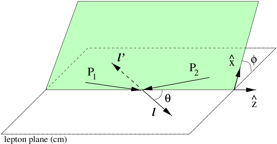
FIG. 1.: Kinematics of the Drell-Yan process in the lepton center of mass frame, for a particular value of $c$.

In this way we arrive at the following expression for the Drell-Yan cross-section in case of unpolarized leptons:

$$\frac{d\sigma(h_{1}h_{2}\to l\bar{l}X)}{d\Omega dx_{1}dx_{2}}=\frac{\alpha^{2}}{3Q^{2}}\;\sum_{a,\bar{a}}e_{a}^{2}\;\Bigg{\{}A(y)\left(f_{1}\overline{f}_{1}-{\lambda_{1}}{\lambda_{2}}g_{1}\overline{g}_{1}\right)$$ (81)

$${}+B(y)\;|\mathchoice{{\hbox{\boldmath$\displaystyle S$}}}{{\hbox{\boldmath$\textstyle S$}}}{{\hbox{\boldmath$\scriptstyle S$}}}{{\hbox{\boldmath$\scriptscriptstyle S$}}}_{1T}|\;|\mathchoice{{\hbox{\boldmath$\displaystyle S$}}}{{\hbox{\boldmath$\textstyle S$}}}{{\hbox{\boldmath$\scriptstyle S$}}}{{\hbox{\boldmath$\scriptscriptstyle S$}}}_{2T}|\;\cos(\phi_{S_{1}}+\phi_{S_{2}})\;\left(h_{1}\overline{h}_{1}\right)$$

$${}+C(y)\;|\mathchoice{{\hbox{\boldmath$\displaystyle S$}}}{{\hbox{\boldmath$\textstyle S$}}}{{\hbox{\boldmath$\scriptstyle S$}}}{{\hbox{\boldmath$\scriptscriptstyle S$}}}_{1T}|\;\sin(\phi_{S_{1}})\;\bigg{(}\frac{2M_{1}}{Q}\,x_{1}\,\left((1-c)f_{T}+c\tilde{f}_{T}\right)\overline{f}_{1}+\frac{2M_{2}}{Q}\,x_{2}\,h_{1}\left(c\overline{h}+(1-c)\tilde{\overline{h}}\right)\bigg{)}$$

$${}+C(y)\;|\mathchoice{{\hbox{\boldmath$\displaystyle S$}}}{{\hbox{\boldmath$\textstyle S$}}}{{\hbox{\boldmath$\scriptstyle S$}}}{{\hbox{\boldmath$\scriptscriptstyle S$}}}_{2T}|\;\sin(\phi_{S_{2}})\;\bigg{(}\frac{2M_{2}}{Q}\,x_{2}\,f_{1}\left(c\overline{f}_{T}+(1-c)\tilde{\overline{f}}_{T}\right)+\frac{2M_{1}}{Q}\,x_{1}\,\left((1-c)h+c\tilde{h}\right)\overline{h}_{1}\bigg{)}$$

$${}+C(y)\;{\lambda_{2}}\;|\mathchoice{{\hbox{\boldmath$\displaystyle S$}}}{{\hbox{\boldmath$\textstyle S$}}}{{\hbox{\boldmath$\scriptstyle S$}}}{{\hbox{\boldmath$\scriptscriptstyle S$}}}_{1T}|\;\cos(\phi_{S_{1}})\;\bigg{(}\frac{2M_{1}}{Q}\,x_{1}\,\big{(}(1-c)g_{T}+c\tilde{g}_{T}\big{)}\overline{g}_{1}+\frac{2M_{2}}{Q}\,x_{2}\,h_{1}\left(c\overline{h}_{L}+(1-c)\tilde{\overline{h}}_{L}\right)\bigg{)}$$

$${}-C(y)\;{\lambda_{1}}\;|\mathchoice{{\hbox{\boldmath$\displaystyle S$}}}{{\hbox{\boldmath$\textstyle S$}}}{{\hbox{\boldmath$\scriptstyle S$}}}{{\hbox{\boldmath$\scriptscriptstyle S$}}}_{2T}|\;\cos(\phi_{S_{2}})\;\bigg{(}\frac{2M_{2}}{Q}\,x_{2}\,g_{1}\left(c\overline{g}_{T}+(1-c)\tilde{\overline{g}}_{T}\right)+\frac{2M_{1}}{Q}\,x_{1}\,\left((1-c)h_{L}+c\tilde{h}_{L}\right)\overline{h}_{1}\bigg{)}\Bigg{\}},$$

where $d\Omega$ = $2dy\,d\phi^{l}$ and $\phi^{l}$ gives the orientation of $\hat{l}_{\perp}^{\mu}\equiv\left(g^{\mu\nu}-\hat{t}^{\{\mu}\hat{t}^{\nu\}}+\hat{z}^{\{\mu}\hat{z}^{\nu\}}\right)l_{\nu}$, the perpendicular part of the lepton momentum $l$, and $y=l^{-}/q^{-}$. In this result we encounter the following functions of $y$:

$$A(y) = \left(1-2y+2y^{2}\right)/2,$$ (82)

$$B(y) = y\,(1-y),$$ (83)

$$C(y) = (1-2y)\,\sqrt{y\,(1-y)}.$$ (84)

Furthermore, $f_{1}\overline{f}_{1}=f_{1}^{a}(x_{1})\overline{f}{}_{1}^{a}(x_{2})$, etc. and where $a$ is the flavor index.

For $c=1/2$ we find agreement with the results of [1] for the cross-section without T-odd distribution functions. Hence, we confirm the deviation of that result from the one found in [15].

We observe single-transverse-spin asymmetries with two possible angular dependences, namely $\sin(\phi_{S_{1}})$ and $\sin(\phi_{S_{2}})$. Each of them comes with two products of functions, in particular an unpolarized one ($f_{1}$ or $h$) times a polarized one ($f_{T}$ or $h_{1}$). There is no choice of $c$ to eliminate the tilde functions from this expression, nor to only retain tilde functions. This shows the non-trivial role of intrinsic transverse momentum of the partons and one cannot discard it. This means that unlike in the case of DIS, one cannot take only $\Phi(x)$ and $\Phi_{D}^{\alpha}(x,y)$ as a basis [12].

If we assume that the presence of T-odd distribution functions is only effective, arising due to gluonic poles, and that $\Phi_{A(\infty)}^{\alpha}=\Phi_{D(\infty)}^{\alpha}$, then $\tilde{f}_{T}^{\text{eff}}=f_{T}^{\text{eff}}$ and $\tilde{h}^{\text{eff}}=h^{\text{eff}}$. This implies the following single spin asymmetry (hadron-two unpolarized), given in the lepton center of mass frame:

$$A_{T}=\frac{2\sin(2\theta)\;\sin(\phi_{S_{1}})}{1+\cos^{2}\theta}\frac{|\mathchoice{{\hbox{\boldmath$\displaystyle S$}}}{{\hbox{\boldmath$\textstyle S$}}}{{\hbox{\boldmath$\scriptstyle S$}}}{{\hbox{\boldmath$\scriptscriptstyle S$}}}_{1T}|}{Q}\sum_{a}e_{a}^{2}\;\bigg{[}2M_{1}\,x_{1}\,f_{T}^{a}(x_{1})f_{1}^{\bar{a}}(x_{2})+2M_{2}\,h_{1}^{a}(x_{1})x_{2}\,h^{\bar{a}}(x_{2})\bigg{]}\Bigg{/}\sum_{a}e_{a}^{2}\;f_{1}^{a}(x_{1})f_{1}^{\bar{a}}(x_{2}),$$ (85)

where we used that $y=(1+\cos\theta)/2$ and $\theta$ is the angle of hadron-two with respect to the momentum of the outgoing leptons. The first term in the asymmetry (proportional to $f_{T}$) is the one discussed in [7] (in their notation it is proportional to $T(x,x)q(y)$), which will also be present in DIS ($f_{1}(x_{2})=\delta(1-x_{2})$). The second term is the other, new single spin asymmetry arising in DY from a gluonic pole. It is not proportional to $T(x,S_{T})$, but to another projection of $\Phi_{F}^{\alpha}$ in the point $x=y$, cf. Eq. (69).

VI Conclusions

We have shown how the effects of so-called gluonic poles in twist-three hadronic matrix elements, which were first discussed by Qiu and Sterman [3, 4], cannot be distinguished from that of T-odd distribution functions. We investigated this for the Drell-Yan process, which is expressed in terms of products of distribution functions. Even in the absence of T-odd distribution functions, imaginary phases arising from hard subprocesses together with gluonic poles give rise to effective T-odd distribution functions. This leads to single spin asymmetries for the Drell-Yan process, such as the one found recently by Hammon et al. [7]. These asymmetries therefore can have a different origin than the analogous asymmetries in inclusive hadron production in $e^{+}e^{-}$ annihilation [23, 24], which can also arise due to final state interactions, which are expected to be present always in contrast to initial state interactions. We have moreover shown that the presence of gluonic poles is in accordance with time-reversal invariance and requires a large distance gluonic field with antisymmetric boundary conditions. Our analysis shows also the role of intrinsic transverse momentum of the partons for the DY cross-section at subleading order.

We thank A. Schäfer for useful discussions. This work was in part supported by the Foundation for Fundamental Research on Matter (FOM) and the National Organization for Scientific Research (NWO). It is also performed in the framework of Grant 96-02-17631 of the Russian Foundation for Fundamental Research and Grant $N^{o}_{-}$ 93-1180 from INTAS.

REFERENCES

[1]
R.D. Tangerman and P.J. Mulders, Phys. Rev. D 51 (1995) 3357;
NIKHEF preprint NIKHEF-94-P7, hep-ph/9408305.
[2]
M. Anselmino, M. Boglione and F. Murgia, Phys. Lett. B 362 (1995) 164.
[3]
J. Qiu and G. Sterman, Phys. Rev. Lett. 67 (1991) 2264.
[4]
J. Qiu and G. Sterman, Nucl. Phys. B 378 (1992) 52.
[5]
V.M. Korotkiyan and O.V. Teryaev, Dubna preprint E2-94-200.
[6]
A.V. Efremov, V.M. Korotkiyan and O.V. Teryaev, Phys. Lett. B 384 (1995) 577.
[7]
N. Hammon, O. Teryaev and A. Schäfer, Phys. Lett. B 390 (1997) 409.
[8]
D.E. Soper, Phys. Rev. D 15 (1977) 1141; Phys. Rev. Lett. 43 (1979) 1847.
[9]
J.P. Ralston and D.E. Soper, Nucl. Phys. B 152 (1979) 109.
[10]
J.C. Collins and D.E. Soper, Nucl. Phys. B 194 (1982) 445.
[11]
H.D. Politzer, Nucl. Phys. B 172 (1980) 349.
[12]
R.K. Ellis, W. Furmanski and R. Petronzio, Nucl. Phys. B 212 (1983) 29.
[13]
A.V. Efremov and O.V. Teryaev, Sov. J. Nucl. Phys. 39 (1984) 962.
[14]
R.L. Jaffe and X. Ji, Phys. Rev. Lett. 67 (1991) 552.
[15]
R.L. Jaffe and X. Ji, Nucl. Phys. B 375 (1992) 527.
[16]
P.J. Mulders and R.D. Tangerman, Nucl. Phys. B 461 (1996) 197;
Nucl. Phys. B 484 (1997) 538 (E).
[17]
O.V. Teryaev, in Proceedings of the 12th International Symposium on
High-Energy Spin Physics, C.W. de Jager et al. (eds), World Scientific
1997, p. 594.
[18]
S. Wandzura and F. Wilczek, Phys. Lett. B 72 (1977) 195.
[19]
J.B. Kogut and D.E. Soper, Phys. Rev. D 1 (1970) 2901.
[20]
A. Schäfer, L. Mankiewicz, P. Gornicki and S. Güllenstern, Phys. Rev. D 47
(1993) R1.
[21]
B. Ehrnsperger, A. Schäfer, W. Greiner, L. Mankiewicz, Phys. Lett. B 321
(1994) 121.
[22]
A.V. Efremov and O.V. Teryaev, Phys. Lett. B 150 (1985) 383.
[23]
W. Lu, Phys. Rev. D 51 (1995) 5305.
[24]
D. Boer, R. Jakob and P.J. Mulders, hep-ph/9702281.
[25]
W. Lu, X. Li, H. Hu, Phys. Lett. B 368 (1996) 281.
[26]
R. Meng, F.I. Olness, and D.E. Soper, Nucl. Phys. B 371 (1992) 79