Abstract

A method to calculate two-loop self-energy diagrams of the Standard Model is demonstrated. A direct physical application is the calculation of the two-loop electroweak contribution to the anomalous magnetic moment of the muon ${\frac{1}{2}(g-2)}_{\mu}$. Presently, we confine ourselves to a “toy” model with only $\mu$, $\gamma$ and a heavy neutral scalar particle (Higgs). The algorithm is implemented as a FORM-based program package. For generating and automatically evaluating any number of two-loop self-energy diagrams, a special C-program has been written. This program creates the initial FORM-expression for every diagram generated by QGRAF, executes the corresponding subroutines and sums up the final results.

PACS number(s): 12.15.Lk, 13.10.+q, 13.40.Em

Keywords: Standard Model, Feynman diagram, recurrence relations,
anomalous magnetic moment

1 Introduction

Recent high precision experiments to verify the Standard Model of electroweak interactions require, on the side of the theory, high-precision calculations resulting in the evaluation of higher loop diagrams. For specific processes thousands of multiloop Feynman diagrams do contribute, and it turns out impossible to perform these calculations by hand. That makes the request for automatization a high-priority task. In this direction, several program packages are elaborated [2, 3, 4, 5]. It appears absolutely necessary that various groups produce their own solutions of handling this problem: various ways will be of different efficiency, have different domains of applicability, and last but not least, should eventually allow for completely independent checks of the final results. This point of view motivated us to seek our own way of automatic evaluation of Feynman diagrams. We have in mind only higher loop calculations (no multipoint functions).

There exist several kinds of methods for evaluating multiloop Feynman diagrams with masses. The most direct and universal method is based on the Feynman parameter representation and subsequent numerical Monte-Carlo integration [6]. The universality is its most essential advancement. Great progress has been achieved in implementing this method into combined automatic systems like GRACE [2]. But the convergence of the Monte-Carlo integration is rather slow, and there is no way to estimate the actual numerical error. When the subintegral expression has kinematical singularities, the error may significantly exceed the estimate [7].

In a semi-analytic method some integrations are done exactly in terms of special functions, and the dimension of numerical integration becomes lower [8], [9]. The advantage of this method is the possibility to deal with tensor structures. However, an essential drawback is the difficulty of consistently performing renormalizations, because one has to stay in the integer dimension.

The method [10] of Taylor expansion of a diagram in external momenta, analytic continuation and Padé-like approximations allows one to recover the behaviour of the function in the whole complex plane of momentum variables. However, it would require the knowledge of rather many expansion coefficients in order to get a sufficiently precise estimate at the threshold.

Therefore, we are going to use the asymptotic expansions of Feynman diagrams in small/large momenta and masses, where the orders of expansion in a small ratio of parameters are completely collected even at the threshold. We are interested in the low-energy physics of the Standard Model. In this situation there exists a natural small parameter: the ratio of the characteristic scale of the process to the scale of the weak interaction, defined by $M_{Z}$. This provides a good convergence for asymptotic expansions of physical observables and, in a number of cases, makes already the leading order sufficient for the existing precision of the experiments. On the other hand, one can use the dimensional renormalization, and then there are no problems with the $R$ operation.

We demonstrate here the functioning of a C program (TLAMM) for the evaluation of the two-loop anomalous magnetic moment (AMM) of the muon ${\frac{1}{2}(g-2)}_{\mu}$. This piloting C program must read the diagrams generated by QGRAF [11] for a given physical process, generate the FORM [12] source code, start the FORM interpreter, read and sum up the results for the class of diagrams under consideration. Here, for the purpose of demonstration, we apply TLAMM to a closed subclass of diagrams of the Standard Model which we refer to as a “toy” model.

Recent papers have reduced the theoretical uncertainty of the muon AMM by partially calculating the two-loop electroweak contributions [13], [14]. In some cases the following approximations were used: terms suppressed by $(1-4\sin^{2}\Theta_{W})$ were omitted; the fermion masses of the first two families were set to zero; diagrams with two or more scalar couplings to the muon, suppressed by the ratio $\frac{m^{2}_{\mu}}{M^{2}_{Z}}$, were discarded; the Kobayashi-Maskawa matrix was assumed to be unity; the mass of the Higgs particle was assumed large as compared to $M_{Z}$.

All of these approximations, except possibly the last one, are well justified and give rise to small corrections only. We consider it of great interest to study also the case $M_{H}\sim M_{Z}$. To perform this calculation is our main physical motivation. Apart from that, for technical reasons, it may be interesting to study the functioning of TLAMM by calculating all $1832$ two-loop diagrams without any approximation.

The calculation of the AMM of the muon reduces, after differentiation and contractions with projection operators, to diagrams of the propagator type with external momentum on the muon mass shell (for details see [15]).

The applicability of the asymptotic expansion [16], [17] in the limit of large masses has to be investigated for diagrams evaluated on the muon mass shell (i.e., $p^{2}=-m_{\mu}^{2}$). Some diagrams already had a threshold at the muon mass shell before the expansion. In other diagrams, this threshold appears in some terms of the expansion. In dimensional regularization, threshold singularities (like any other infrared singularities if they are strong enough) manifest themselves as poles in $\varepsilon$ (in $4-2\varepsilon$ dimensions). They ought to cancel for the total AMM. We check this for a closed subset of diagrams in the toy model.

2 Large-mass expansion

The asymptotic expansion in the limit of large masses is defined [17] as

$$F_{G}(q,M,m,\varepsilon)\stackrel{{\scriptstyle M\to\infty}}{{\sim}}\sum_{\gamma}F_{G/\gamma}(q,m,\varepsilon)\circ T_{q^{\gamma},m^{\gamma}}F_{\gamma}(q^{\gamma},M,m^{\gamma},\varepsilon)$$ (1)

where $G$ is the original graph, $\gamma$’s are subgraphs involved in the asymptotic expansion, $G/\gamma$ denotes shrinking $\gamma$ to a point; $F_{\gamma}$ is the Feynman integral corresponding to $\gamma$; $T_{q_{\gamma},m_{\gamma}}$ is the Taylor operator expanding the integrand in small masses $\{m_{\gamma}\}$ and small external momenta $\{q_{\gamma}\}$ of the subgraph $\gamma$ (before integration); “$\circ$” inserts the subgraph expansion in the numerator of the integrand $F_{G/{\gamma}}$. The sum goes over all subgraphs $\gamma$ which (a) contain all lines with large masses, and (b) are one-particle irreducible relative to lines with light or zero masses.

The following types of integrals occur in the asymptotic expansion of the muon AMM in the Standard Model:

1. two-loop tadpole diagrams with various heavy masses on internal lines;

2. two-loop self-energy diagrams, involving contributions from fermions lighter or heavier than the muon, with the external momentum on the muon mass shell;

3. two-loop self-energy diagrams with two or three muon lines and the external momentum on the muon mass shell;

4. various products of a one-loop self-energy diagram on shell and a one-loop tadpole with a heavy mass.

Almost all of these diagrams can be evaluated analytically using the package SHELL2 [18]. For our calculation we have modified this package in the following way:

1. There are no restrictions on the indices of the lines (powers of scalar denominators).

2. More recurrence relations are used, and the dependence on the space-time dimension is always explicitly reducible to powers of linear factors.

3. A new algorithm for simplification of this rational fractions is implemented. These modifications essentially reduce the execution time (in some cases, down to the order of a hundredth).

4. New programs for evaluating two-loop tadpole integrals with different masses are added.

5. New programs were written for the asymptotic expansion of one-loop self-energy diagrams (relevant for renormalization) in the large-mass limit.

3 The toy model

As the first step, we concentrate on a “toy” model, a “slice” of the Standard Model, involving a light charged spinor $\Psi$, the photon $A_{\mu}$, and a heavy neutral scalar field $\Phi$. The scalar has triple $\left(g\right)$ and quartic $\left(\lambda\right)$ self-interactions, and the Yukawa coupling $\left(y\right)$ to the spinor. The Lagrangian of the toy model reads (in the Euclidean space-time)

$${\it L} = \frac{1}{2}\partial_{\mu}\Phi\partial^{\mu}\Phi+\frac{1}{2}M^{2}:\Phi^{2}:-\frac{g}{3!}:\Phi^{3}:-\frac{\lambda}{4!}:\Phi^{4}:+\frac{1}{4}\left(\partial_{\mu}A_{\nu}-\partial_{\nu}A_{\mu}\right)^{2}$$ (2)

$$+\frac{1}{2\alpha}\left(\partial_{\mu}A^{\mu}\right)^{2}+\bar{\Psi}\left(\hat{\partial}+m\right)\Psi+ie\bar{\Psi}\hat{A}\Psi-y\Phi\bar{\Psi}\Psi$$

where $e$ is the electric charge and $\alpha$ is a gauge fixing parameter.

The main aims of the present investigation are the following:

1. Verification of the consistency of the large-mass asymptotic expansion with the external momentum on the mass shell of a small mass. In particular, we check the cancelation of all threshold singularities that appear in individual diagrams and manifest themselves as infrared poles in $\varepsilon$.

2. Estimation of the influence of a heavy neutral scalar particle on the AMM of the muon in the framework of the Standard Model.

3. Verification of gauge independence (we use the covariant gauge with an arbitrary parameter $\alpha$).

In what follows we analyze in some detail the diagrams contributing to the AMM of the fermion in our toy model and specify the renormalization procedure. Apart from counterterms $40$ diagrams contribute to the two-loop AMM of the fermion. After performing the Dirac and Lorentz algebra, all diagrams can be reduced to some set of scalar prototypes. A prototype defines the arrangement of massive and massless lines in a diagram. Individual integrals are specified by the powers of the scalar denominators, called indices of the lines. From the point of view of the asymptotic expansion method the topology of the diagram is essential. All diagrams of the toy model that contribute to the two-loop AMM can be classified in terms of $9$ prototypes (we omit the pure QED diagrams). These prototypes and their corresponding subgraphs $\gamma$ involved in the asymptotic expansion, are given in Fig.1. In dimensional regularization, the last subgraphs vanish in cases $1,4,7$, and $8$, owing to massless tadpoles.

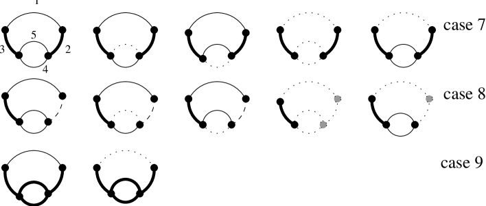
Figure 1: The prototypes and their subgraphs contributing to the large mass expansion. Thick, thin and dashed lines correspond to the heavy-mass, light-mass, and massless propagators, respectively. Dotted lines indicate the lines omitted in the subgraph $\gamma$.

4 Program TLAMM

All diagrams are generated in symbolic form by means of QGRAF [11]. For automatic calculation we have created a special piloting program written in C. This program, called TLAMM,

1. reads QGRAF output;

2. creates a file containing the complete FORM program for calculating each diagram;

3. executes FORM;

4. reads FORM output, picks out the result of the calculation, and builds the total sum of all diagrams in a single file which can be processed by FORM.

The program has its own internal notation for topologies. In the problem $g-2$ of a lepton in the Standard Model there are four different topologies (see Fig.2). Line number 1 is always assumed to correspond to a fermion line (a lepton or a neutrino); therefore, topologies b and c are distinguished.

Figure 2: Two-loop topologies existing for the AMM of the lepton in the Standard Model.

All diagrams are classified according to their local prototypes. The notation consists of a letter (the topology) and five (or four in B case) integer numbers specifying the masses on the lines

0 for the zero mass: $\gamma$, $\nu$;

1 for a mass less than $m_{\mu}$: $e,u,d$;

2 for $m_{\mu}$;

3 for an intermediate mass between $m_{\mu}$ and $M_{W}$: $s,\tau,c,b$;

4 for a heavy mass: $W,Z,t,H$.

In the Feynman gauge $\alpha=1$ all pseudo-Higgs particles and the Faddeev-Popov ghosts are heavy except for one massless ghost.

Each local prototype is calculated by means of the asymptotic expansion in heavy masses. For each diagram the corresponding FORM subroutine is called according to the local prototype.

Identifiers for vertices and propagators and the explicit Feynman rules are red from separate files and then inserted into the FORM program. Because the number of identifiers needed for the calculation of all diagrams together may exceed the FORM capacity, the piloting program TLAMM retains for each diagram only those involved in its calculation.

All initial settings are defined in a configuration file. The latter contains information on the file names, identifiers of topologies, the distribution of momenta, and the description of the model in terms of the notation that is some extension of QGRAF’s. The program carries out the complete verification of all input files except the QGRAF output.

There exist several options which allow one to process only the diagrams

• explicitly listed by number;

• of a given prototype;

• of a specified topology.

There are also some debugging options.

The asymptotic expansion of each prototype is performed by a separate FORM program. For efficiency of the algorithm the following points are essential:

1. The result of the calculation is presented as a series in small parameters. Care is taken to avoid the production of unnecessarily high powers in intermediate results.

2. For the evaluation of the Feynman integrals, it is necessary to reduce scalar products of momenta in the numerator to the square combinations which are present in the denominator. Most efficiently this is done by means of recurrence relations proposed by Tarasov [19].

As a demonstration of the functioning of TLAMM, the unrenormalized (“bare”) contributions of all the two-loop diagrams to the anomalous magnetic moment of the fermion in the toy model are presented in Figs.3–7 to the leading order in $m^{2}/M^{2}$. In the presented expressions the factor of $(2\pi)^{-4}$ is implied. During the calculations, each loop was divided by $\Gamma(1+\varepsilon)$ rather than multiplied by $\Gamma(1-\varepsilon)$ as is done in the $\overline{\rm{MS}}$ definition.

Figure 3: The two-loop QED contributions to the AMM in the arbitrary gauge.

Figure 4: The two-loop AMM contributions proportional to $y^{4}$.

Figure 5: The two-loop AMM contributions proportional to $e^{2}y^{2}$ (to be continued).

Figure 6: The two-loop AMM contributions proportional to $e^{2}y^{2}$ (continued).

Figure 7: The two-loop AMM contributions involving the triple interaction $g$ .

5 The results of the calculations

Initially, we use the minimal subtraction scheme for the parameters of the Lagrangian (2). Afterwards, it is more convenient to re-express the running masses $m_{R}$ and $M_{R}^{2}$ in terms of the physical pole masses $m,M^{2}$ of the particles (at the one-loop level, relevant here),

$$m_{R}(\mu^{2}) = m\Big{\{}1-\frac{e_{R}^{2}}{16\pi^{2}}\Big{(}4-3\ln\frac{m^{2}}{\mu^{2}}\Big{)}+\frac{y_{R}^{2}}{16\pi^{2}}\Big{[}\frac{5}{4}-\frac{3}{2}\ln\frac{M^{2}}{\mu^{2}}$$ (3)

$$+ \left(\frac{m^{2}}{M^{2}}\right)\Big{(}\frac{1}{6}-\ln\frac{M^{2}}{m^{2}}\Big{)}+\left(\frac{m^{2}}{M^{2}}\right)^{2}\Big{(}\frac{7}{8}-\frac{3}{2}\ln\frac{M^{2}}{m^{2}}\Big{)}$$

$$+ \left(\frac{m^{2}}{M^{2}}\right)^{3}\Big{(}\frac{47}{20}-3\ln\frac{M^{2}}{m^{2}}\Big{)}+\cdots\Big{]}\Big{\}},$$

$$M_{R}^{2}(\mu^{2}) = M^{2}\Big{\{}1+\frac{y_{R}^{2}}{16\pi^{2}}\Big{[}4-2\ln\frac{M^{2}}{\mu^{2}}-\left(\frac{m^{2}}{M^{2}}\right)\Big{(}16-12\ln\frac{M^{2}}{\mu^{2}}\Big{)}$$ (4)

$$- \left(\frac{m^{2}}{M^{2}}\right)^{2}\Big{(}18+12\ln\frac{M^{2}}{m^{2}}\Big{)}+\left(\frac{m^{2}}{M^{2}}\right)^{3}\Big{(}\frac{4}{3}-8\ln\frac{M^{2}}{m^{2}}\Big{)}+\cdots\Big{]}$$

$$+ \frac{g_{R}^{2}}{16\pi^{2}M^{2}}\Big{(}1-\frac{\pi}{2\sqrt{3}}-\frac{1}{2}\ln\frac{M^{2}}{\mu^{2}}\Big{)}\Big{\}},$$

thus terming to the on-shell renormalization of the masses. The scalar-field tadpoles do never contribute owing to the normal ordering of the Lagrangian. Anyway, their contributions would become of no consequence after everything is expressed in terms of the pole masses. As a result, the quartic interaction constant $\lambda$ falls out of the two-loop anomalous magnetic moment of the fermion.

We have calculated the asymptotic expansion up to the $7$th order in the ratio $m^{2}/M^{2}$ and have convinced ourselves that all orders of the expansion are free from on-shell singularities and involve only the logarithms of the masses. For brevity, we present just two leading orders

$$a_{\mu} = \frac{e_{R}^{2}}{4\pi^{2}}\left[\frac{1}{2}\right]+\frac{e_{R}^{4}}{16\pi^{4}}\left[\frac{197}{144}+\left(\frac{1}{2}-3\ln\left(2\right)\right)\zeta\left(2\right)+\frac{3}{4}\zeta\left(3\right)+\frac{1}{6}\ln\frac{m^{2}}{\mu^{2}}\right]$$ (5)

$$+\frac{y_{R}^{2}}{16\pi^{2}}\left(\frac{m}{M}\right)^{2}\left[-\frac{7}{3}+2\ln\frac{M^{2}}{m^{2}}\right]$$

$$+\frac{e_{R}^{2}y_{R}^{2}}{64\pi^{4}}\left(\frac{m}{M}\right)^{2}\left[\frac{335}{27}+\frac{121}{9}\ln\frac{M^{2}}{\mu^{2}}-\frac{179}{18}\ln\frac{m^{2}}{\mu^{2}}\right.$$

$$\left.-\frac{13}{2}\ln^{2}\frac{M^{2}}{\mu^{2}}-\frac{7}{2}\ln^{2}\frac{m^{2}}{\mu^{2}}+10\ln\frac{M^{2}}{\mu^{2}}\ln\frac{m^{2}}{\mu^{2}}-29\zeta\left(2\right)\right]$$

$$+\frac{y_{R}^{3}}{256\pi^{4}}\left(\frac{g_{R}m}{M^{2}}\right)\left[2-\frac{4}{3}\zeta\left(2\right)+\left(\frac{m}{M}\right)^{2}\left\{\frac{46}{3}-\frac{189}{2}S_{2}+6\ln\frac{M^{2}}{m^{2}}\right\}\right]$$

$$+\frac{y_{R}^{2}}{256\pi^{4}}\left(\frac{g_{R}m}{M^{2}}\right)^{2}\left[-\frac{5}{3}+\frac{45}{2}S_{2}-\frac{13}{6}\frac{\pi}{\sqrt{3}}-\left(2-\frac{\pi}{\sqrt{3}}\right)\ln\frac{M^{2}}{m^{2}}\right]$$

$$+\frac{y_{R}^{4}}{256\pi^{4}}\left(\frac{m}{M}\right)^{2}\left[\frac{103}{6}+13\ln\frac{m^{2}}{\mu^{2}}-\frac{74}{3}\ln\frac{M^{2}}{\mu^{2}}+10\ln\frac{M^{2}}{\mu^{2}}\ln\frac{M^{2}}{m^{2}}\right],~{}$$

where $S_{2}=\frac{4}{9\sqrt{3}}{\rm Cl}_{2}\left(\frac{\pi}{3}\right)=0.2604341$ with ${\rm Cl}_{2}$ the Clausen function; $e_{R},y_{R}$ and $g_{R}$ are renormalized (running) coupling constants.

In quantum electrodynamics it is agreed to express the running charge of the electron $e_{R}(\mu^{2})$ in terms of the experimentally measurable physical charge $e$. The later is defined by the nonrelativistic Thompson limit of the Compton scattering, that is, as the product of the on-shell vertex function at the zero momentum of the photon [with the projection operator $\left(-i\hat{p}+m\right)$ $\gamma_{\mu}$ $\left(-i\hat{p}+m\right)$ ] by the on-shell wave-function renormalization constant (the residue of the fermion propagator at its pole). Both quantities are renormalization- and gauge-invariant but contain an infrared singularity which cancels in the product. Performing an analogous procedure for the charge of the muon in our toy model to the one-loop order we get

$$e_{R}^{2}(\mu^{2})=e^{2}\left(1-\frac{1}{3}\frac{e^{2}}{4\pi^{2}}\ln\frac{m^{2}}{\mu^{2}}\right).$$ (6)

The physical Yukawa charge could also be defined in terms of the on-shell Yukawa vertex. However, its evaluation is a difficult task in itself. On the other hand, in the Standard Model the Yukawa charge is usually related to the mass of the fermion rather than kept as an independent parameter. As a compromise, to define the physical Yukawa charge $y$, we use the following one-loop expression for the running charge:

$$y_{R}^{2}(\mu^{2})=y^{2}\left(1+\frac{3}{2}\frac{e^{2}}{4\pi^{2}}\ln\frac{m^{2}}{\mu^{2}}-5\frac{y^{2}}{16\pi^{2}}\ln\frac{M^{2}}{\mu^{2}}\right).$$ (7)

The calculation through the on-shell vertex would generally give a finite correction (independent of $\mu^{2}$) to this formula. The running of the triple scalar interaction is inessential in the approximation that we consider. In terms of the physical charges, the anomalous magnetic moment (5) becomes

$$a_{\mu} = \frac{e^{2}}{4\pi^{2}}\left[\frac{1}{2}\right]+\frac{e^{4}}{16\pi^{4}}\left[\frac{197}{144}+\left(\frac{1}{2}-3\ln\left(2\right)\right)\zeta\left(2\right)+\frac{3}{4}\zeta\left(3\right)\right]$$ (8)

$$+\frac{y^{2}}{16\pi^{2}}\left(\frac{m}{M}\right)^{2}\left[-\frac{7}{3}+2\ln\frac{M^{2}}{m^{2}}\right]$$

$$+\frac{e^{2}y^{2}}{64\pi^{4}}\left(\frac{m}{M}\right)^{2}\left[\frac{335}{27}+\frac{121}{9}\ln\frac{M^{2}}{m^{2}}-\frac{13}{2}\ln^{2}\frac{M^{2}}{m^{2}}-29\zeta\left(2\right)\right]$$

$$+\frac{y^{3}}{256\pi^{4}}\left(\frac{gm}{M^{2}}\right)\left[2-\frac{4}{3}\zeta\left(2\right)+\left(\frac{m}{M}\right)^{2}\left\{\frac{46}{3}-\frac{189}{2}S_{2}+6\ln\frac{M^{2}}{m^{2}}\right\}\right]$$

$$+\frac{y^{2}}{256\pi^{4}}\left(\frac{gm}{M^{2}}\right)^{2}\left[-\frac{5}{3}+\frac{45}{2}S_{2}-\frac{13}{6}\frac{\pi}{\sqrt{3}}-\left(2-\frac{\pi}{\sqrt{3}}\right)\ln\frac{M^{2}}{m^{2}}\right]$$

$$+\frac{y^{4}}{256\pi^{4}}\left(\frac{m}{M}\right)^{2}\left[\frac{103}{6}-13\ln\frac{M^{2}}{m^{2}}\right].$$

The Standard-model motivated values for the Yukawa and triple scalar interactions are

$$y=-\frac{1}{2}\frac{e}{\sin\Theta_{W}}\frac{m_{\mu}}{M_{W}},\hskip 42.67912ptg=-\frac{e}{\sin\Theta_{W}}\frac{3M_{H}^{2}}{2M_{W}}.$$ (9)

Then, the estimate of the influence of a heavy neutral scalar particle on the anomalous magnetic moment of the muon is (besides the pure QED contribution)

$$\Delta a_{\mu} = \frac{e^{2}}{4\pi^{2}}\frac{1}{\sin^{2}\Theta_{W}}\left(\frac{m_{\mu}}{M_{W}}\right)^{2}\left(\frac{m_{\mu}}{M_{H}}\right)^{2}\Biggl{[}\Biggl{(}-\frac{7}{48}+\frac{1}{8}\ln\left(\frac{M_{H}}{m_{\mu}}\right)^{2}\Biggr{)}$$ (10)

$$+ \frac{e^{2}}{4\pi^{2}}\Biggl{(}\frac{335}{432}+\frac{121}{144}\ln\left(\frac{M_{H}}{m_{\mu}}\right)^{2}-\frac{13}{32}\ln^{2}\left(\frac{M_{H}}{m_{\mu}}\right)^{2}-\frac{29}{16}\zeta\left(2\right)\Biggr{)}$$

$$+ \frac{e^{2}}{4\pi^{2}}\frac{1}{\sin^{2}\Theta_{W}}\left(\frac{M_{H}}{M_{W}}\right)^{2}\Biggl{(}-\frac{9}{256}-\frac{1}{64}\zeta\left(2\right)+\frac{405}{512}S_{2}$$

$$-\frac{39}{256}\frac{\pi}{\sqrt{3}}+\frac{9}{128}\left(\frac{\pi}{\sqrt{3}}-1\right)\ln\left(\frac{M_{H}}{m_{\mu}}\right)^{2}\Biggr{)}$$

$$+ \frac{e^{2}}{4\pi^{2}}\frac{1}{\sin^{2}\Theta_{W}}\left(\frac{m_{\mu}}{M_{W}}\right)^{2}\Biggl{(}\frac{379}{1536}-\frac{567}{512}S_{2}+\frac{5}{256}\ln\left(\frac{M_{H}}{m_{\mu}}\right)^{2}\Biggr{)}\Biggr{]}.$$

This contribution is strongly suppressed and seems improbable to be exhibited in future experiments.

We conclude that

1. the gauge independence of the two-loop contribution to the anomalous magnetic moment of the fermion has been verified;

2. any threshold singularities in the on-shell asymptotic expansion of the diagrams contributing to the AMM do cancel;

3. the correction due to the heavy neutral scalar is suppressed by the ratio of $m^{4}_{\mu}$ to heavy masses.

Acknowledgments This work was supported in part by the RFFI grant # 96-02-17531, by Volkswagenstiftung and by Bundesministerium für Forschung und Technologie.

References

- [1] L. V. Avdeev, J. Fleischer, M. Yu. Kalmykov and M. N. Tentyukov, ”Towards Automatic Analytic Evaluation of Massive Feynman Diagrams”, (hep-ph/9610467).
- [2] T. Ishikawa et al., Minami-Taeya group “GRACE manual”, KEK-92-19, 1993.
- [3] J. Kublbeck, M. Böhm and A. Denner, Comp. Phys. Comm. 60 (1990), 165. R. Mertig, M. Böhm and A. Denner, Comp. Phys. Comm. 64 (1991), 345.
- [4] E. E. Boos, M. N. Dubinin, V. A. Ilyin, A. E. Pukhov and V. I. Savrin, ”COMPHEP: specialized package for automatic calculations of elementary particle decays and collisions”, SNUTP 94-116 (1994) (hep-ph/9503280).
- [5] T. van Ritbergen, J. A. M. Vermaseren, S. A. Larin and P. Nogueira, Int. J. Mod. Phys. C 6 (1995) 513-518.
- [6] J. Fujimoto, Y. Shimizu, K. Kato and Y. Oyanagi, Prog. Theor. Phys. 87 (1992) 1233; J. Fujimoto, Y. Shimizu, K. Kato and T. Kaneko, Int. J. Mod. Phys. C 6 (1995) 525.
- [7] P. A. Baikov and D. J. Broadhurst, in New Computing Techniques in Physics Research IV, p.167 (hep-ph/9504398).
- [8] D. Kreimer, Phys. Lett. B273 (1991), 277; ibid B292 (1992), 341.
- [9] F. A. Berends and J. B. Tausk, Nucl. Phys. B421 (1994), 456. A. Czarnecki, U. Kilian and D. Kreimer, Nucl. Phys. B433 (1995), 259. S. Bauberger, F. A. Berends, M. Böhm and M. Buza, Nucl. Phys. B434 (1995), 383. S. Bauberger, and M. Böhm, Nucl. Phys. B445 (1995), 25.
- [10] J. Fleischer and O. V. Tarasov, Z.Phys. C64 (1994), 413; J. Fleischer, Int. J. Mod.Phys. C6 (1995), 495.
- [11] P. Nogueira, J. Comput. Phys. 105 (1993), 279.
- [12] J. A. M. Vermaseren, Symbolic manipulation with FORM, Amsterdam, Computer Algebra Nederland, 1991.
- [13] T. V. Kukhto, E. A. Kuraev, A. Schiller and Z. K. Silagadze, Nucl. Phys. B371 (1992), 567; E. A. Kuraev, T. V. Kukhto, and A. Schiller, Sov. J. Nucl. Phys. 51 (1990), 1031.
- [14] S. Peris, M. Perrottet and E. de Rafael, Phys. Lett. B355 (1995), 523. A. Czarnecki, B. Krause and W. Marciano, Phys. Rev. D52 (1995), R2619; Phys. Rev. Lett. 76 (1996), 3267. A. Czarnecki and B. Krause, ”Computing techniques for two-loop corrections to anomalous magnetic moments of lepton”, Preprint hep-ph/9611241.
- [15] R. Z. Roskies, E. Remiddi and M. J. Levine in Quantum Electrodynamics, p. 163, ed. T. Kinoshita (World Scientific, Singapore, 1990).
- [16] F. V. Tkachov, Institute for Nuclear Research preprint, P-0332, ”Euclidean Asymptotics of Feynman integrals: Basic notations.”, Moscow (1983); P-0358, ”Asymptotics of Euclidean Feynman integrals. 2. one loop case.”, Moscow (1984); Int. J. Mod. Phys. A8 (1993), 2047; S. G. Gorishny, Nucl. Phys. B319 (1989), 633. K. G. Chetyrkin and V. A. Smirnov, Institute for Nuclear Research preprint, P-0518, ”Asymptotic expansions of Feynman amplidudes, -operation and the method of glueing”, (in Russian), Moscow (1987); S. G. Gorishny and S. A. Larin, Nucl. Phys. B283 (1987), 452; K. G. Chetyrkin, Teor. Math. Phys. 75 (1988), 26; ibid 76 (1988), 207; Max-Planck-Institute preprint, MPI-PAE/PTh-13/91, ”Combinatorics of , and operations and asymptotic expansions of Feynman integrals in the limit of large momenta and masses”, Munich (1991); G. B. Pivovarov and F. V. Tkachov, Int. J. Mod. Phys. A8 (1993), 2241.
- [17] V. A. Smirnov, Comm. Math. Phys. 134 (1990), 109; Renormalization and asymptotic expansions (Bikrhäuser, Basel, 1991); Phys. Lett. B 394 (1997), 205. A. Czarnecki and V. A. Smirnov, Phys. Lett. B 394 (1997), 211.
- [18] J. Fleischer and O. V. Tarasov, Comp. Phys. Commun. 71 (1992), 193.
- [19] O.V. Tarasov, in New Computing Techniques in Physics Research IV, ed. B. Denby and D. Perret-Gallix (World Scientific, Singapore, 1995), p.161 (hep-ph/9505277).