Soft photons and hard thermal loops

Abstract

We calculate within the Hard Thermal Loop expansion the production rate of soft photons and lepton pairs by a hot quark-gluon plasma at thermal equilibrium, up to the 2-loop order. Strong collinear divergences appear to mix the orders of the perturbative expansion so that the 2-loop order is in fact dominant compared to the 1-loop order. More precisely, angular integrals that would otherwise be of order 1 are found to behave as powers of $1/g$ when the produced photon is massless, therefore breaking the standard HTL power counting rules.

ENSLAPP-A-665, hep-ph/9710203

1 Introduction

The production rate of photons or dileptons is of some relevance to the phenomenology of a quark-gluon plasma. Indeed, these electromagnetic probes are interacting very slightly through electromagnetic forces. Therefore, it is expected that they will escape the plasma without re-interacting after their creation. As a consequence, they are rather clean probes of the state of the system at the time it produced them.

Among the theoretical tools to calculate such observables, one can quote the semi-classical methods based on an eikonal approximation [1, 2, 3, 4], and the tools of finite temperature field theory [5, 6, 7, 8, 9, 10]. In this report, I focus mainly on the field theoretical method. I assume a plasma in thermal equilibrium and sufficiently hot so that the temperature is much larger than the masses of the particles. From the theoretical point of view, studying these production rates is a good test of our present understanding of problems such as infrared and collinear singularities in high temperature QCD.

The starting point is to connect the photon production rate to the imaginary part of the photon polarization tensor, via the following two relations [5, 11]:

$${\rm At\ }Q^{2}=0{\rm,}\qquad{{dN}\over{dtd^{3}{\tenimbf x}}}=-{{d^{3}{\tenimbf q}}\over{(2\pi)^{3}}}\;{{n_{{}_{B}}(q_{o})}\over{q_{o}}}{\rm Im}\,\Pi^{\mu}{}_{\mu}(q_{o},{\tenimbf q})$$ (1)

$${\rm At\ }Q^{2}>0{\rm,}\qquad{{dN}\over{dtd^{3}{\tenimbf x}}}=-\alpha{{dq_{o}d^{3}{\tenimbf q}}\over{12\pi^{3}}}\;{{n_{{}_{B}}(q_{o})}\over{Q^{2}}}{\rm Im}\,\Pi^{\mu}{}_{\mu}(q_{o},{\tenimbf q})\;.$$ (2)

Basically, these two formulae differ only by the allowed phase space, by the coupling constant involved in the decay of a virtual photon into a lepton pair and by the propagator of such a heavy photon.

2 Infrared problems and hard thermal loops

2.1 Origin of the problem

Before going on with some details of the calculation we performed, it is worth recalling some of the issues related to the concept of hard thermal loops (HTL) [12], and its relevance to the problem of infrared divergences. Indeed, although HTLs have been introduced to solve the problem of the apparent non gauge invariance of the gluon damping rate [13], they proved to be quite efficient in improving the infrared behavior of thermal gauge theories, which is a priori more severe than at $T=0$ due to the singular behavior of Bose-Einstein’s factors at small energies:

$$n_{{}_{B}}(l_{o})={1\over{e^{l_{0}/T}-1}}\approx{T\over{l_{o}}}\gg 1\quad{\rm if\ }l_{o}\ll T\;.$$ (3)

Since in the Feynman rules, these factors are always accompanied by the Dirac’s distribution $\delta(l_{o}^{2}-{\tenimbf l}^{2}-m^{2})$, the Bose-Einstein’s weights are a problem only if there are massless bosons in the theory. In QCD, one has gluons…

2.2 Semantics: hard and soft scales

Figure 1: Hard and soft scales.

It is useful in thermal field theories to distinguish between two typical energy scales: particles of energy of order $T$ are said to be hard, and particles of energy of order $gT$ are said to be soft. Roughly speaking, the hard scale is the typical energy of partons in the plasma, and the soft scale is the typical energy of quanta exchanged during parton interactions.

2.3 Summation of hard thermal loops

The foundations of the HTL concept lie in the fact that some one-loop diagrams have a thermal contribution which is dominated by the hard region of phase space, and moreover this thermal contribution is as large as the bare corresponding function when all its external legs carry soft momenta. For instance, this is what happens for the one-loop photon self-energy in QED.

Figure 2: Hard thermal loop of the photon self energy.

Then, in order to take these large contributions into account, one defines an effective field theory [14, 15] by the means of effective propagators and vertices. The effective propagators are obtained by a Dyson summation of the HTL contribution to the corresponding self energy, whereas the effective vertices are defined to be the sum of their bare counterpart plus the HTL contribution to the corresponding vertex function. In order to avoid double counting of thermal corrections, one should include counter-terms whose purpose is to subtract at higher orders what had been added by this summation. In that way, the overall Lagrangian function remains unchanged, so that the use of this effective theory just amounts to a re-ordering of the perturbative expansion.

2.4 Basic properties

The HTLs have a few nice properties that make the effective theories obtained by they summation rather attractive:

$\bullet$ The HTLs are gauge invariant. As a consequence, the effective theory one obtains by summing all the HTLs is also gauge invariant. It is important to note the fact that the effective vertices are essential here to achieve the gauge invariance of the effective Lagrangian. In fact, starting by the summation of 2-point HTLs in order to obtain a better behaved effective propagator, one can obtain all the $n-$point $(n\geq 3)$ HTLs by the requirement that the effective theory should be gauge invariant [14].

$\bullet$ The common physical interpretation of the HTLs is that they reflect the long distance behavior of the gauge interaction better than the bare theory did. In particular, they account for the Debye screening phenomenon, which is translated in field theory by the fact that the gluon acquires an effective mass $m_{{}_{D}}\sim gT$, thus leading to a screened interaction whose range is of order $m_{{}_{D}}^{-1}$.

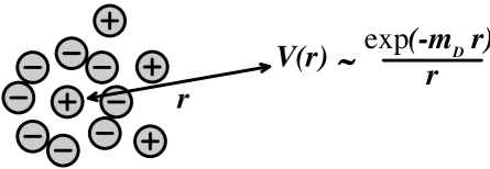
Figure 3: QED Debye screening.

$\bullet$ The $n-$point $(n\geq 3)$ HTLs are vanishing if one takes the trace over the Lorentz indices of two external gauge bosons.

$\bullet$ Another property which makes the HTLs simple is the fact that the 1-loop diagrams that give the HTLs are calculated with massless particles running in the loop. Besides the technical simplification this fact provides, it is also at the origin of collinear singularities encountered when one is using HTLs with light-like external legs.

2.5 Further problems

Despite the great improvement the HTLs provide for perturbative calculations in thermal gauge theories, some nasty problems remain.

$\bullet$ The first one is the problem of collinear singularities evocated above. Due to the fact that the HTLs are calculated with massless propagators running in the hard loop, these functions are divergent when at least one of the external legs is on-shell. This is due to an angular integral like:

$$\int{{d\Omega_{\tenimbf p}}\over{\widehat{P}\cdot K}}\propto\int\limits_{-1}^{+1}{{d\cos\theta}\over{k(1-\cos\theta)}}=\infty\;,$$ (4)

where $\widehat{P}\equiv(1,\hat{\tenimbf p})$, and $K$ is a light-like external momentum. A possible solution to this problem has been proposed recently [16], which amounts to keep an asymptotic thermal mass for the particle running in the hard loop. Obviously, the previous divergent integral becomes now:

$$\int{{d\Omega_{\tenimbf p}}\over{\widehat{P}\cdot K}}\propto\int\limits_{-1}^{+1}{{d\cos\theta}\over{\omega_{k}-k\cos\theta}}<\infty\;,$$ (5)

where $\omega_{k}\equiv\surd({\tenimbf k}^{2}+m^{2})$. Moreover, it has been shown that these improved hard thermal loops still generate a gauge invariant effective theory.

$\bullet$ The other problem which is not solved by the summation of HTLs is due to the fact that static transverse gauge bosons don’t get a thermal mass. This property is known to be true to all orders in QED, in which case it is related to the fact that static magnetic fields are not screened in a plasma. In QCD, there is still a hope that self-interactions of gluons can generate such a mass for the transverse modes, but it seems that this mass will be beyond the abilities of perturbative methods, and at most of order $g^{2}T$ contrary to usual thermal masses that are of order $gT$. The nullity of this magnetic mass is at the origin of further infrared divergences, like those encountered in the perturbative calculation of the damping rate of a fast fermion.

3 $\gamma$ production rate at $1$ loop

3.1 1-loop diagrams and results

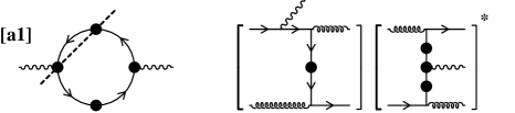
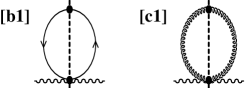
Figure 4: Contributions to the photon production rate at 1-loop in the effective theory. The first one is accompanied by the corresponding physical amplitudes. Black dots denote effective propagators and vertices.

These 1-loop diagrams have been evaluated by several groups [5, 6, 7, 8], leading to the following results:

$${\rm Im}\,\Pi^{\mu}{}_{\mu}{}_{|{\tenimbf[a1]}}(q_{o},{\tenimbf q})\sim e^{2}g^{4}{{T^{3}}\over{q_{o}}}\;,$$ (6)

$${\rm Im}\,\Pi^{\mu}{}_{\mu}{}_{|{\tenimbf[b1]}}(q_{o},{\tenimbf q})=0\;,\qquad{\rm Im}\,\Pi^{\mu}{}_{\mu}{}_{|{\tenimbf[c1]}}(q_{o},{\tenimbf q})=0\;.$$ (7)

The result given for the diagram $[{\tenimbf a1}]$ is to be preceded by a numerical coefficient which is finite if the emitted photon is massive $(Q^{2}>0)$, but that diverges logarithmically when the photon mass goes to zero. This is due to the fact that the hard loop contained in the effective $\gamma q\bar{q}$ vertex is plagued by a collinear divergence when one of its external legs is light-like. If one applies the prescription presented in the previous section, this coefficient becomes a number of order $\ln(1/g)$.

3.2 Comments

A few remarks are worth saying concerning these results:

$\bullet$ The only non-vanishing contribution at 1-loop in the effective theory based on the summation of the HTLs comes from the diagram $[{\tenimbf a1}]$ and corresponds to the interference between the two amplitudes represented in the figure 4. If, instead of using thermal field theory, one had just tried to guess what are the dominant processes contributing to photon production by a hot plasma, it is unlikely that these processes would have been thought as being dominant.

$\bullet$ The exact nullity of the diagrams $[{\tenimbf b1}]$ and $[{\tenimbf c1}]$ is a consequence of the remark made earlier concerning the trace over Lorentz indices of $n-$point HTLs.

$\bullet$ In the case of the diagram $[{\tenimbf a1}]$, taking the trace $\cdots{}^{\mu}{}_{\mu}$ doesn’t make the result vanish, but nevertheless is at the origin of a suppression by a power of $g$. Therefore, if this suppression is specific to this topology, it may be that some 2-loop diagrams are of the same order (in thermal field theories the expansion parameter is $g$ instead of $g^{2}$).

This fact, added to the oddity of the dominant physical process at 1-loop, should incite one to evaluate the 2-loop contributions.

4 $\gamma$ production rate at $2$ loops

4.1 2-loop diagrams

In the list of 2-loop diagrams contributing to the photon production rate, we skipped right from the beginning those having a tadpole topology since taking the $\cdots{}^{\mu}{}_{\mu}$ trace will make them exactly cancel. Moreover, we skipped topologies containing effective vertices like $\gamma ggg$ or $\gamma gq\bar{q}$. This will be justified later by the fact that the topologies $[{\tenimbf a2}]$ and $[{\tenimbf b2}]$ are important because of quasi superposed collinear singularities (leading to an enhancement by powers of $1/g$), whereas the diagrams we skipped can have at most powers of $\ln(1/g)$. For the remaining diagrams, it is a priori essential to keep the topologies with counter-terms in order to avoid double counting of thermal corrections already included at the 1-loop level. Nevertheless, it is obvious that the diagrams with counter-terms are of the order of magnitude of $[{\tenimbf a1}]$ (the counter-term is part of the effective vertex contained in $[{\tenimbf a1}]$).

Figure 5: Some 2-loop contributions to photon production. The cross denote HTL counter-terms.

4.2 Physical processes

Looking more carefully at the kinematics of these 2-loop diagrams, we can see that the dominant contribution comes from the region of phase space where the quark running in the loop is hard while the exchanged gluon is soft. As a consequence, we can approximate the effective vertices by their bare counterpart, and the effective quark propagators by their hard approximation:

$${\cal S}(P)=i{{p_{o}\gamma^{o}-\omega_{+}(p)\hat{\tenimbf p}\cdot{\bf\gamma}}\over{p_{o}^{2}-\omega_{+}^{2}(p)+i\epsilon}}\;,$$ (8)

with $\omega_{+}(p)\equiv\surd({\tenimbf p}^{2}+M_{{}_{F}}^{2})$, where $M^{2}_{{}_{F}}\equiv g^{2}C_{{}_{F}}T^{2}/4$. Therefore, we can replace the diagrams $[{\tenimbf a2}]$ and $[{\tenimbf b2}]$ by the simpler version of the figure 6, where we used a slightly abusive notation for the quark propagators we represented as bare ones whereas we are retaining an asymptotic thermal mass in them.

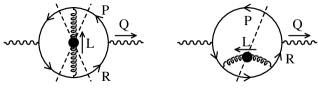
Figure 6: Simplified version of $\tenimbf[a2]$ and $\tenimbf[b2]$.

On the same figure, we also represented the cuts relevant to the calculation of the imaginary part of the polarization tensor. The cuts not represented always imply that the quark be soft, which would drastically reduce the phase space available. A priori, by cutting an effective gluon propagator, we can pick the pole part $(L^{2}>0)$ or the Landau damping part $(L^{2}<0)$ of the gluon spectral function. The two contributions correspond respectively to photon production by Compton effect or by bremsstrahlung, which looks more intuitive than the processes involved in $[{\tenimbf a1}]$.

Figure 7: Physical processes involved in $\tenimbf[b2]$.

4.3 Collinear behavior

If both the external photon and the internal quark are massless, the diagrams $[{\tenimbf a2}]$ and $[{\tenimbf b2}]$ exhibits a collinear singularity when the 3-momentum of the quark is collinear to that of the external photon. Moreover, contrary to the case of the diagram $[{\tenimbf a1}]$ where such singularities are at most logarithmic, we have here two denominators (corresponding to the propagators which are not cut) that vanish almost simultaneously. This is obvious in the case of the diagram $[{\tenimbf a2}]$ for which we have an exact double pole due to the insertion of the self-energy correction. In the case of the diagram $[{\tenimbf b2}]$, both denominators are distinct and so are the two poles. At $Q^{2}=0$, $R^{2}$ is vanishing when $\tenimbf p$ is parallel to $\tenimbf q$, and $(P+L)^{2}$ is vanishing when ${\tenimbf r}+{\tenimbf l}$ is parallel to $\tenimbf q$. Nevertheless, since $\tenimbf p$ and $\tenimbf r$ are hard whereas $\tenimbf q$ and $\tenimbf l$ are soft, these two conditions of collinearity are satisfied almost at the same time. It means that the two poles are very close, so that their association behaves almost like a double pole.

Therefore, in both $[{\tenimbf a2}]$ and $[{\tenimbf b2}]$, we have denominators that lead to a linear collinear divergence. A careful calculation of the angular integral while keeping $Q^{2}\geq 0$ and the quark thermal mass $M_{{}_{F}}$ indicates that these divergences are regularized by the combination $M^{2}_{\rm eff}\equiv M^{2}_{{}_{F}}+Q^{2}r^{2}/q_{o}^{2}$ divided by $T^{2}$. If we limit ourselves to photons of very small virtuality $(Q^{2}\ll q_{o}^{2})$, then this dimensionless regulator is much smaller than $1$, and the dimensionless angular integral is much larger than $1$, which would be its order of magnitude in the absence of collinear problems. In fact, at $Q^{2}=0$, the only scale in the angular integral is $M^{2}_{{}_{F}}/T^{2}\sim g^{2}$, so that the enhancement factor of this integral is $1/g^{2}$. The fact that powers of $1/g$ can appear at $Q^{2}=0$ in the perturbative expansion due to collinear singularities can make the order of magnitude of a diagram somewhat unpredictable by the power counting rules associated usually with the HTL expansion (indeed, these rules always assume that the dimensionless angular integrals that one can factorize out of the HTLs are of order $1$, and we have shown by this example that these integrals can sometimes be as large as powers of $1/g$).

The above results concerning the order of magnitude of the angular integrals indicate that the result is completely dominated by the collinear sector of the phase space. As a consequence, one can use a collinear approximation to obtain a simplified expression for the Dirac’s algebra associated with the quark loop. The results one obtains that way are:

$${\rm Tr}_{\tenimbf[a2]}\approx 16Q^{2}P_{\alpha}P_{\beta}\;,\qquad{\rm Tr}_{\tenimbf[b2]}\approx 16(Q^{2}-L^{2})P_{\alpha}P_{\beta}\;,$$ (9)

where $\alpha$ and $\beta$ are the Lorentz indices of the gluon. Then, limiting ourselves to very small $Q^{2}$, we can neglect the contribution of the diagram $[{\tenimbf a2}]$.

Moreover, since we have the constraint $\delta(P^{2}-M^{2}_{{}_{F}})$, the denominator $(P+L)^{2}-M^{2}_{{}_{F}}$ can approach zero only if $L^{2}$ is negative. As a consequence, the portion of phase space that contains the collinear singularities also verifies $L^{2}<0$, which indicates that the bremsstrahlung production of photons dominates with respect to the Compton effect.

4.4 Results

Therefore, the result we obtain for the imaginary part of the polarization tensor of the photon can take the form [9, 10]:

$${\rm Im}\,\Pi^{\mu}{}_{\mu}(q_{o},{\tenimbf q})\approx-{{e^{2}g^{2}NC_{{}_{F}}}\over{3\pi^{2}}}\sum\limits_{T,L}\,J_{{}_{T,L}}\,{{T^{3}}\over{q_{o}}}\;,$$ (10)

where the quantities $J_{{}_{T,L}}$ are pure numbers quantifying the respective contributions of transverse and longitudinal gluons exchange. These coefficients are given by an integral which is evaluated numerically, as a function of the ratio $Q^{2}/q_{o}^{2}$ and plotted on the figure 8. We can see clearly an enhancement in the region of small $Q^{2}$. Indeed, since the regularization of collinear divergences is realized by the mass $M^{2}_{\rm eff}$, increasing with $Q^{2}$, the result is larger at small $Q^{2}$.

Figure 8: Transverse and longitudinal contributions as a function of $Q^{2}/q_{o}^{2}$, for $3$ colors and $3$ light flavors. The value taken for the coupling constant is $g=0.44$.

The same quantities are plotted also with a logarithmic scale that enables one to see in more detail the region of small $Q^{2}$. In particular, we see that they converge to finite values when $Q^{2}$ goes to $0$. Moreover, we see that the enhancement effect (quantified by the ratio of the values taken at $Q^{2}=0$ and at $Q^{2}\sim q_{o}^{2}$) is larger when $g$ is small.

Figure 9: Effect of the value of the coupling constant. Solid lines: $g=0.1$, dashed lines: $g=0.44$, dotted lines: $g=2$. We used $3$ colors and $3$ light flavors.

Let us now list a few important features of the result we obtained:

$\bullet$ The diagram $[{\tenimbf a1}]$, only non vanishing contribution at the 1-loop order, is negligeable compared to $[{\tenimbf b2}]$, for small enough $Q^{2}$ $(Q^{2}\ll q_{o}^{2}\ll T^{2})$. Moreover, the latter is much larger than the diagrams with counter-terms of the figure 5. This fact is due to strong collinear divergences. Therefore, there is a possibility that such collinear singularities may invalidate the perturbative expansion since powers of the inverse coupling constant emerge in the process.

$\bullet$ The result we obtained is free of any infrared divergence and is totally insensitive to the magnetic mass scale as long as the magnetic mass is negligeable in front of the thermal mass $M_{{}_{F}}$. If this condition is satisfied, then the regularization of potential IR singularities in the transverse gluon contribution is done by the quark mass $M_{{}_{F}}$. There is a natural explanation for this a priori surprising property related to the fact that the delta function constraints become incompatible in the limit $L\to 0$ when $M_{{}_{F}}>0$.

$\bullet$ Our result can be put into a form that looks like the expressions obtained by semi-classical methods:

$${{dN}\over{dtd^{3}{\tenimbf x}}}\approx {{d^{3}{\tenimbf q}}\over{(2\pi)^{3}2q_{o}}}\int\prod\limits_{i=1,2}{{d^{4}P_{i}}\over{(2\pi)^{4}}}\;2\pi\delta(P_{i}^{2}-M_{{}_{F}}^{2})\;n_{{}_{F}}(p^{o}_{i})$$ (11)

$$\times\int\prod\limits_{i=1,2}{{d^{4}P^{\prime}_{i}}\over{(2\pi)^{4}}}\;2\pi\delta(P^{\prime}_{i}{}^{2}-M_{{}_{F}}^{2})\,[1-n_{{}_{F}}(p^{\prime}_{i}{}^{o})]$$

$$\times\left|{\cal M}\right|^{2}(P_{1},P_{2};P^{\prime}_{1}+Q,P^{\prime}_{2})\;\;\;(2\pi)^{4}\delta(P_{1}+P_{2}-P^{\prime}_{1}-P^{\prime}_{2}-Q)$$

$$\times e^{2}\sum_{{\rm pol.\ }\epsilon}\left({{P_{1}\cdot\epsilon}\over{P_{1}\cdot Q}}-{{P^{\prime}_{1}\cdot\epsilon}\over{P^{\prime}_{1}\cdot Q}}\right)^{2}\;.$$

The interpretation of the various factors entering the above formula is rather easy: starting from the beginning, we find the photon phase space, the phase space of two incoming quarks, the phase space of the same outgoing quarks, the amplitude $|{\cal M}|^{2}$ of the scattering process between the two quarks, associated to a delta constraint ensuring the overall momentum conservation, and finally a factor which is the square of the electromagnetic current coupling the photon to the quark line.

Therefore, we see that thermal field theory gives the same kind of expression as the one obtained by semi-classical methods [1, 2, 3, 4] when considering the photon emission induced by a single scattering. In fact, the thermal field theory result is more precise in the sense that it has not neglected the contribution of transverse gluons, which is as important as the longitudinal one as can be seen from the curves plotted above.

5 Conclusions and perspectives

The study of the photon production rate by a hot quark-gluon plasma by using the effective theory based on the summation of the hard thermal loops has shown that serious problems may arise from strong collinear singularities. More precisely, angular integrals that are usually assumed to be of order unity in the HTL framework are found to behave as powers of $1/g$. It is not known by now if such singularities or even stronger ones may emerge from higher order contributions, enabling them to remain at the same level.

From a more phenomenological point of view, we arrived at the conclusion that real or slightly virtual soft photons are mostly produced by bremsstrahlung in a hot plasma.

An important issue is to determine whether higher order contributions, corresponding to photon emission induced by multiple scatterings, are important or not. The importance of this study is related to the fact that the semi-classical methods predict that multiple scatterings are important and can modify the photon spectrum in the region of small energy, a phenomenon known as the Landau-Pomeranchuk-Migdal effect.

References

- [1] J. Cleymans, V.V. Goloviznin, K. Redlich, Phys. Rev. D 47, 173 (1993).
- [2] J. Cleymans, V.V. Goloviznin, K. Redlich, Phys. Rev. D 47, 989 (1993).
- [3] R. Baier, Y.L. Dokshitzer, A.H. Mueller, S. Peigne, D. Schiff, Nucl. Phys. B 478, 577 (1996).
- [4] R. Baier, Y.L. Dokshitzer, A.H. Mueller, S. Peigne, D. Schiff, Nucl. Phys. B 483, 291 (1997).
- [5] E. Braaten, R.D. Pisarski, T.C. Yuan, Phys. Rev. Lett. 64, 2242 (1990).
- [6] R. Baier, S. Peigne, D. Schiff, Z. Phys. C 62, 337 (1994).
- [7] P. Aurenche, T. Becherrawy, E. Petitgirard, Preprint ENSLAPP-A-452/93, hep-ph/9403320.
- [8] S.M.H. Wong, Z. Phys. C 53, 465 (1992).
- [9] P. Aurenche, F. Gelis, R. Kobes, E. Petitgirard, Phys. Rev. D 54, 5274 (1996).
- [10] P. Aurenche, F. Gelis, R. Kobes, E. Petitgirard, Z. Phys. C 75, 315 (1997).
- [11] H.A. Weldon, Phys. Rev. D 28, 2007 (1983).
- [12] E. Braaten, R.D. Pisarski, Nucl. Phys. B 337, 569 ( 1990).
- [13] E. Braaten, R.D. Pisarski, Phys. Rev. D 42, 2156 (1990).
- [14] E. Braaten, R.D. Pisarski, Phys. Rev. D 45, 1827 (1992).
- [15] J. Frenkel, J.C. Taylor, Nucl. Phys. B 374, 156 (1992).
- [16] F. Flechsig, A.K. Rebhan, Nucl. Phys. B 464, 279 (1996).