$\gamma$ - beam propagation in the anisotropic medium

Abstract

Propagation of $\gamma$-beam in the anisotropic medium is considered. The simplest example of such a medium of the general type is a combination of the two linearly polarized monochromatic laser waves with different frequencies (dichromatic wave). The optical properties of this combination are described with the use of the permittivity tensor. The refractive indices and polarization characteristics of normal electromagnetic waves propagating in the anisotropic medium are found. The relations, describing variations of $\gamma$ -beam intensity and Stokes parameters as functions of the propagation length, are obtained. The influence of laser wave intensity on the propagation process is calculated.

The $\gamma$-beam intensity losses in the dichromatic wave depend on the initial circular polarization of $\gamma$-quanta. This effect is also applied to single crystals which are oriented in some regions of coherent pair production. In principle, the single crystal sensitivity to a circular polarization can be used for determination of polarization of high energy ( in tens GeV and more) $\gamma$-quanta and electrons.

1 Introduction

Polarization effects [1, 2] arising from the visible light propagation in the anisotropic or gyrotropic medium are well-known. The theory [3] makes prediction about the analogous effects for $\gamma$-quanta with energy $>1$ GeV propagating in single crystals, which present the anisotropic medium. The main absorption process of $\gamma$-quanta in the single crystals is the electron-positron pair production. The cross section of this process depends on the linear polarization of $\gamma$-beam with respect to crystallographic planes. As a result, the monochromatic linearly polarized $\gamma$-beam may be presented as a superposition of two electromagnetic waves with different refractive indices due to which the transformation of linear (circular) polarization to circular (linear) one takes place.

On the other hand, the process of $e^{+}e^{-}$-pair production in single crystals is similar to the same process in a linearly polarized laser wave [4]. A possibility to use a bunch of linearly polarized laser photons as a ”single crystal” is pointed in [5], but the concrete calculations of this possibility are not given.

In the recent paper [6] it has been shown that the polarization effects such as birefringence and rotation of polarization plane for $\gamma$- beams with energies of tens GeV or more take place for short (about some picoseconds) laser bunches and parameters of lasers, which may be provided by real techniques. In the cited paper the differential equations which determine the variation of Stokes parameters and intensity of $\gamma$-quanta traversing a bunch of arbitrary polarized laser photons are obtained. For these calculations the well-known scattering amplitudes for the process of elastic scattering light by light [7, 8] were used. Then in paper [9] the process of $\gamma$-beam propagation in the field of a laser wave was investigated with the use of traditional optical methods. Bisides, the transformation of $\gamma$-beam linear polarization into circular in the anisotropic medium was discussed in [10].

The case of $\gamma$-quanta propagation in single crystals described in [3] is a special case of such a process. The general case of $\gamma$-propagation in single crystals oriented in the angle region corresponding to process of the coherent pair production was considered in Ref.([5]). In this paper it was shown that the propagating $\gamma$-beam is a superposition of the two elliptically polarized waves but the description of variation of the $\gamma$-beam polarization is unavailaible.

In the present paper we study the general case of high energy $\gamma$-quanta propagation through the anisotropic medium. The anisotropic medium is determined as such a medium, which optical properties may be described using a symmetric permittivity tensor [1, 2]. As will be indicated the simplest example of the anisotropic medium of the general type is a superposition of the two linearly polarized laser waves with different frequencies moving in the same direction. We will study in detail the $\gamma$-quanta propagation in such a combined laser wave with the goal of better understanding of this process in more complicated cases, as in single crystals.

2 Permittivity tensor in anisotropic medium

We write the equations of the electromagnetic field in a medium ($\gamma$-beam propagating in a laser wave, single crystal, and the like) in the following form [1, 2]

$$rot\vec{B}={{1}\over{c}}{{\partial\vec{D}}\over{\partial t}}\,,\;\;\;div\vec{D}=0\,,$$

$$rot\vec{E}=-{{1}\over{c}}{{\partial\vec{B}}\over{\partial t}}\,,\;\;\;div\vec{B}=0\,,$$ (1)

$\vec{E}$ - is the intensity of electric field and $\vec{D}$ and $\vec{B}$ are the electric and magnetic induction vectors, t is the time , c is the speed of light. All the properties of the medium are reflected in the relation between $\vec{B},\vec{E}$ and $\vec{D}$. Eqs.(1) would suffice to describe the $\gamma$-beam propagation in a medium and such a property as the intensity of magnetic field is not needed [1, 2]. We represent the relation between $\vec{D}$ and $\vec{E}$ in the form

$$D_{i}(\omega)=\varepsilon_{ij}E_{j}(\omega)\,,\;\;\;(i,j=1,2,3)\,,$$ (2)

where $\varepsilon_{ij}=\varepsilon^{\prime}_{ij}+i\varepsilon^{\prime\prime}_{ij}$ is the complex permittivity tensor and $\omega$ is the frequency of $\gamma$-quanta.

By way of example of the anisotropic medium let us consider the superposition of the two linearly polarized laser waves, moving in the same direction. The frequencies of these waves (photon energies) are different. In order to determine the permittivity tensor in the case of a monochromatic field (high energy $\gamma$-beam) $\vec{E}_{0}e^{i(\vec{k}\vec{r}-\omega t)}$ propagating in above-mentioned laser medium , where $\vec{k}$ is the wave vector of the $\gamma$-quanta, we find the average energy lost by the electromagnetic wave per unit volume $V$ and per unit time [1, 2]

$$\tilde{q}={1\over{4\pi V}}\int_{V}\vec{E}{{\partial\vec{D}}\over{\partial t}}dV={{i\omega}\over{16\pi}}(\varepsilon_{ij}^{\ast}-\varepsilon_{ji})E_{j}^{\ast}E_{i}\,.$$ (3)

The mechanism by which the wave loses energy is $e^{+}e^{-}$-pair production in the field of the laser wave [11]. The process is determined primarily by the transverse part of the permittivity tensor, while the longitudinal components of the tensor are higher-order infinitesimals in the interaction constant $\alpha$ [4, 12]. Taking this into account, and in the coordinate system one axis of which is oriented parallel to the wave vector of $\gamma$-quanta, we have from (3)

$$\tilde{q}={{i\omega J}\over{4}}\{({\varepsilon_{11}}^{\ast}-\varepsilon_{11})(1+\xi_{3})+({\varepsilon_{12}}^{\ast}-\varepsilon_{21})(\xi_{1}-i\xi_{2})+({\varepsilon_{21}}^{\ast}-\varepsilon_{12})(\xi_{1}+i\xi_{2})+$$

$$({\varepsilon_{22}}^{\ast}-\varepsilon_{22})(1-\xi_{3})\}\,,$$ (4)

where $J=(E_{1}{E_{1}}^{\ast}+E_{2}{E_{2}}^{\ast})/8\pi,\xi_{i}$ are Stokes parameters of $\gamma$-beam. On the other hand, knowing the cross section $\sigma_{\gamma\gamma}$ of the pair production process, we can write

$$\tilde{q}=2cJ\{n_{l,1}\sigma_{\gamma\gamma,1}+n_{l,2}\sigma_{\gamma\gamma,2}\}\,,$$ (5)

where $n_{l,1}$ is the number of photons per volume unit of the laser wave with the linear polarization equals $P_{l,1}$, and $n_{l,2}$ is the similar number for second wave with the linear polarization equals $P_{l,2}$, $\sigma_{\gamma\gamma,1}$ and $\sigma_{\gamma\gamma,2}$ are corresponding cross sections for $e^{+}e^{-}$ -pair production in $\gamma\gamma$ -interactions, $P_{1,1},P_{3,1}$ and $P_{1,2},P_{3,2}$ are the Stokes parameters of the laser waves ($P_{1,1}^{2}+P_{3,1}^{2}=P_{l_{1}}^{2},\,P_{1,2}^{2}+P_{3,2}^{2}=P^{2}_{l_{2}}$). Factor 2 in this formula is due to the counter-motion of the $\gamma$-beam and laser wave. Note, that the Eq.(5) is true, when the intensity of laser wave are not high (see below).

We can write the cross section of $e^{+}e^{-}$-pair production in the following form [4, 6, 7, 11]

$$\sigma_{\gamma\gamma}(z)=\sigma_{0}(z)+\sigma_{l}(z)(\xi_{1}P_{1}+\xi_{3}P_{3})\,,\,\;0<z\leq 1\,,$$ (6)

$$\sigma_{0}(z)=\pi r_{e}^{2}z\{(1+z-z^{2}/2)L_{\_}-\sqrt{1-z}(1+z)\}\,,$$ (7)

$$\sigma_{l}(z)={\pi r_{e}^{2}z^{3}\over 2}(L_{\_}+2\sqrt{1-z}/z)\,,$$ (8)

$$L_{\_}=\ln{{1+\sqrt{1-z}}\over\ {1-\sqrt{1-z}}}\,$$

where $z={{m^{2}c^{4}}\over{E_{\gamma}E_{l}}}$ is the invariant variable, $E_{\gamma}$ is the $\gamma$-quantum energy, $m$ and $r_{e}$ are the mass and classical radius of electron, $E_{l}$ and $P_{1},P_{3}$ are the energy and Stokes parameters of the laser photon. It is well known that the pair production is a threshold process and, because of this, the laser wave is a transparent medium for $\gamma$-beam , when $E_{\gamma}E_{l}<m^{2}c^{4}$ or $z>1$. There are two different photon energies $E_{l,1}$ and $E_{l,2}$ in the case of dichromatic laser wave. Because of this, it is convenient to use the two corresponding invariant variable $z_{1}={{m^{2}c^{4}}\over{E_{\gamma}E_{l,1}}}$ and $z_{2}={{m^{2}c^{4}}\over{E_{\gamma}E_{l,2}}}$. It is evident that $z_{1}/z_{2}=E_{l,2}/E_{l,1}$. Comparing Eqs.(4) and (5) we can find the components of permittivity tensor caused by $\gamma$-quanta absorption.

Then we can determine the other components of the tensor with the help of the following dispersion relations [2]

$$\varepsilon^{\prime}_{ij}-\delta_{ij}={2\over\pi}{\cal P}\int_{0}^{\infty}{{x\varepsilon^{\prime\prime}_{ij}(x)\,dx}\over{x^{2}-\omega^{2}}}\,,$$ (9)

$$\varepsilon^{\prime\prime}_{ij}=-{{2\omega}\over{\pi}}{\cal P}\int_{0}^{\infty}{{(\varepsilon^{\prime}_{ij}-\delta_{ij})\,dx}\over{x^{2}-\omega^{2}}}\,,$$ (10)

where $\delta_{ij}$ is the Kronecker $\delta$-function. Comparing Eqs.(4) and (5), we get

$$\varepsilon^{\prime\prime}_{11}+\varepsilon^{\prime\prime}_{22}=4c(n_{l,1}\sigma_{0}(z_{1})+n_{l,2}\sigma_{0}(z_{2}))/\omega\,,$$ (11)

$$\varepsilon^{\prime\prime}_{11}-\varepsilon^{\prime\prime}_{22}=4c(n_{l,1}\sigma_{l}(z_{1})P_{3,1}+n_{l,2}\sigma_{l}(z_{2})P_{3,2})/\omega\,,$$ (12)

$$\varepsilon^{\prime\prime}_{12}+\varepsilon^{\prime\prime}_{21}=4c(n_{l,1}\sigma_{l}(z_{1})P_{1,1}+n_{l,2}\sigma_{l}(z_{2})P_{1,2})/\omega\,,$$ (13)

$$\varepsilon^{\prime}_{12}=\varepsilon^{\prime}_{21}$$ (14)

It easy to verify that $\varepsilon_{12}=\varepsilon_{21}$. The same result is evident from the theory of generalized receptivity [13].

The other components of the permittivity tensor can be calculated with the help of relations (9 )-(10). The results of calculations of the components $\varepsilon_{ij}$ for the arbitrary coordinate system, one axis of which is oriented parallel to the wave vector of the $\gamma$-quanta, are presented below

$$\varepsilon^{\prime}_{11}-\varepsilon^{\prime}_{22}={\alpha\over{2\pi E_{o}^{2}}}(<E^{2}_{1}>P_{3,1}z^{2}_{1}{F_{1}}^{\prime}(z_{1})+<E^{2}_{2}>P_{3,2}z^{2}_{2}{F_{1}}^{\prime}(z_{2}))$$ (15)

$$\varepsilon^{\prime}_{11}+\varepsilon^{\prime}_{22}=2+{2\alpha\over{\pi E_{o}^{2}}}(<E_{1}^{2}>z^{2}_{1}{F_{2}}^{\prime}(z_{1},1)+<E_{2}^{2}>z^{2}_{2}{F_{2}}^{\prime}(z_{2},1))\,,$$ (16)

$$\varepsilon^{\prime}_{12}=\varepsilon^{\prime}_{21}={\alpha\over{4\pi E_{o}^{2}}}(<E^{2}_{1}>P_{1,1}z^{2}_{1}{F_{1}}^{\prime}(z_{1})+<E^{2}_{2}>P_{1,2}z^{2}_{2}{F_{1}}^{\prime}(z_{2}))$$ (17)

$$\varepsilon^{\prime\prime}_{11}-\varepsilon^{\prime\prime}_{22}=-{\alpha\over 4E_{o}^{2}}(<E^{2}_{1}>P_{3,1}{F_{1}}^{\prime\prime}(z_{1})+<E^{2}_{2}>P_{3,2}{F_{1}}^{\prime\prime}(z_{2}))\,,$$ (18)

$$\varepsilon^{\prime\prime}_{11}+\varepsilon^{\prime\prime}_{22}={\alpha\over E_{o}^{2}}(<E^{2}_{1}>{F_{2}}^{\prime\prime}(z_{1},1)+<E^{2}_{2}>{F_{2}}^{\prime\prime}(z_{2},1)\,,$$ (19)

$$\varepsilon^{\prime\prime}_{12}=\varepsilon^{\prime\prime}_{21}=-{\alpha\over 8E_{o}^{2}}(<E^{2}_{1}>P_{1,1}{F_{1}}^{\prime\prime}(z_{1})+<E^{2}_{2}>P_{1,2}{F_{1}}^{\prime\prime}(z_{2}))\,,$$ (20)

where $<E^{2}_{i}>=4\pi n_{l,i}E_{l,i}\,(i=1,2)$ is the mean square of intensity electric field for every laser wave and the functions $F^{\prime}_{1},F^{\prime}_{2},F^{\prime\prime}_{1},F^{\prime\prime}_{2},$ are equal to:

$${F_{1}}^{\prime}(z)=\cases{[\sqrt{1-z}+{z\over 2}L_{-}]^{2}+[\sqrt{1+z}-{z\over 2}L_{+}]^{2}-{{\pi^{2}z^{2}}\over{4}},\;0<z\leq 1,\cr-[\sqrt{z-1}-z\mathop{\rm arcctg}\nolimits\sqrt{z-1}]^{2}+[\sqrt{1+z}-{z\over 2}L_{+}]^{2},\;z>1.\cr}$$ (21)

$${F_{2}}^{\prime}(z,\mu)=\cases{-2-\mu-(1+\mu(z-{z^{2}\over 2})){1\over 4}L^{2}_{-}-(1-\mu(z+{z^{2}\over 2})){1\over 4}L^{2}_{+}+\cr+{{(1+\mu z)\sqrt{1-z}}\over{2}}L_{-}-{{(\mu z-1)\sqrt{z+1}}\over{2}}L_{+}+{\pi^{2}\over 4}(1+\mu(z-{{z^{2}}\over 2})),\;0<z\leq 1,\cr-2-\mu+(1+\mu(z-{z^{2}\over 2}))\mathop{\rm arcctg}\nolimits^{2}(\sqrt{z-1})-(1-\mu(z+{z^{2}\over 2})){1\over 4}L^{2}_{+}+\cr+(1+\mu z)\sqrt{z-1}\mathop{\rm arcctg}\nolimits\sqrt{z-1}-{{(\mu z-1)\sqrt{1+z}}\over{2}}L_{+},\;z>1.\cr}$$ (22)

$${F_{1}}^{\prime\prime}(z)=\cases{z^{4}(L_{-}+{{2\sqrt{1-z}}\over{z}}),\;0<z\leq 1,\cr 0,\;z>1.\cr}$$ (23)

$${F_{2}}^{\prime\prime}(z,\mu)=\cases{z^{2}((1+\mu(z-{z^{2}\over 2}))L_{-}-\sqrt{1-z}(1+\mu z)),\;0<z\leq 1,\cr 0,\;z>1\cr}$$ (24)

The function $L_{+}$ is equal to:

$$L_{+}=ln{{\sqrt{1+z}+1}\over{\sqrt{1+z}-1}}\,.$$

The constant $E_{o}={{m^{2}c^{3}}\over{e\hbar}}$ is the critical field of quantum electrodynamics. The presented here data completely determine the permittivity tensor for high energy $\gamma$-quanta traversing a dichromatic linearly polarized bunch of laser photons.

In a number of problems in optics it is more convenient to employ the tensor $\eta_{ij}$ , which is inverse of the tensor $\varepsilon_{ij}$. When $|\varepsilon_{ij}-\delta_{ij}|\ll 1$, these tensors are related by

$$\eta_{ij}+\varepsilon_{ij}=2\delta_{ij}.$$ (25)

It should be noted the following peculiarities of the permittivity tensor:

1) Our description can be extended to the case when the laser bunch is superposition more then two linearly polarized waves. It is obvious that the analogous terms should be added in the tensor components in these cases.

2) Let us that $E_{l,1}>E_{l,2}$. Then the laser bunch is a transparent medium at $z_{1}>1$. In this case the all components $\varepsilon^{\prime\prime}_{ij}$ are equal to zero.

3) In the general case the symmetric complex tensor $\varepsilon^{\prime\prime}_{ij}$ does not reduce to principal axes [1, 2, 5] (i.e., there does not exist a coordinate system in which the tensors $\varepsilon^{\prime}_{ij}$ and $\varepsilon^{\prime\prime}_{ij}$ are simultaneously diagonal).

4)In the case, when the two waves have the same direction of linear polarization or their polarizations are orthogonal, the tensor $\varepsilon_{ij}$ can be reduced to a diagonal form. The permittivity tensor for monochromatic linearly polarized wave can be reduced to the diagonal form for the all time.

Everything said above is also true for tensor $\eta_{ij}$.

3 Refractive indices of $\gamma$-quanta

The main problem of optic of anisotropic medium is to investigate the propagation of monochromatic plane waves, characterized by definite values of the frequency $\omega$ and wave vector $\vec{k}$. Such waves, satisfying a homogeneous wave equation, are called normal electromagnetic waves [2], and they have the form

$$\vec{E}=\vec{E}_{0}e^{i(\vec{k}\vec{r}-\omega t)},\vec{k}=\omega\tilde{n}\vec{s}/c\,,$$

where $\vec{E}_{0}$ is the complex vector, independent of coordinates $\vec{r}$ and time, $\tilde{n}$ is the complex index of refraction and $\vec{s}=\vec{k}/|k|$ is a real unit vector. The vectors $\vec{D}$ and $\vec{B}$ have the same form.

From Maxwell’s equations (1) we obtain the wave equation

$$rotrot\vec{E}+{1\over c}{{\partial^{2}\vec{D}}\over{\partial t^{2}}}=0\,.$$

Taking into account the relation between $\vec{D}$ and $\vec{E}$ in a system of coordinates in which the axis $x$ is oriented parallel to the wave vector, we obtain

$$\eta_{11}{{\partial^{2}D_{1}}\over{\partial x^{2}}}+\eta_{12}{{\partial^{2}D_{2}}\over{\partial x^{2}}}-{1\over c^{2}}{{\partial^{2}D_{1}}\over{\partial t^{2}}}=0,$$

$$\eta_{21}{{\partial^{2}D_{1}}\over{\partial x^{2}}}+\eta_{22}{{\partial^{2}D_{2}}\over{\partial x^{2}}}-{1\over c^{2}}{{\partial^{2}D_{2}}\over{\partial t^{2}}}=0.$$ (26)

For a monochromatic plane wave it follows from these equations that

$$(\tilde{n}^{-2}\delta_{ij}-\eta_{ij})D_{j}=0,\;i,j=1,2.$$ (27)

From the condition that the two homogeneous equations are compatible, we find the index of refraction of the $\gamma$-quanta

$$\tilde{n}^{-2}={S\over 2}\pm\sqrt{{S^{2}\over 4}-D_{\eta}}=(\eta_{11}+\eta_{22})/2\pm\sqrt{(\eta_{11}-\eta_{22})^{2}/4+\eta_{12}\eta_{21}}\,,$$ (28)

where $S$ and $D_{\eta}$ are, respectively, the trace and determinant of the matrix $\eta_{ij}$. Thus, in the general case the $\gamma$-beam propagates through the laser wave as the superposition of two electromagnetic waves with different refractive indices. Note, that the two roots of (29) which have form $-1+small\;quantity$, are superfluous. They correspond to the $\gamma$-quanta motion in the reverse direction.

In the general case the refractive indices are complex values. However, they are real values, when the laser bunch is a transparent medium for $\gamma$-quantum (all components of the permittivity tensor are real number in this case). Fig.1 illustrates the refractive indices as functions of the invariant variable $z$ (the laser wave parameters are in the caption).

4 Polarization properties of $\gamma$-beam propagation in laser wave

Here we consider the polarization properties one of two normal electromagnetic waves. From dispersion equations (28) we find the ratios of the components of the vector $\vec{D}$

$${D_{1}\over D_{2}}=\kappa={{\tilde{n}^{-2}-\eta_{22}}\over{\eta_{21}}}={{|D_{1}|}\over{|D_{2}|}}e^{i\delta},$$ (29)

where $\delta$ is the phase shift between $D_{1}$ and $D_{2}$. This ratio $\kappa$ can be reduced to zero or to the form $\kappa=i\rho$ (since $|D_{1}||D_{2}|\sin\delta=b_{1}b_{2}$, where $b_{1}$ and $b_{2}$ are the semiaxes of the ellipse and $|\rho|=b_{1}/b_{2}$ [14]) by the rotation of the coordinate system around the wave vector of $\gamma$-quanta (the $x$-axis is constantly aligned with the wave vector). The first case corresponds to the propagation of a linearly polarized wave and the second case corresponds to an elliptically polarized wave; in addition, $\rho>0(\rho<0)$ corresponds to left (right) - hand polarization of $\gamma$-quanta.

The different cases of $\gamma$-beam propagation in anisotropic medium, which optical properties described by the symmetric tensor, were considered in paper [5]. In the case when permittivity tensor may be reduce to principal axes (i.e., there is a coordinate system in which $\varepsilon_{12}=0$) the normal electromagnetic waves are linearly polarized. In general case the permittivity tensor does not reduce to principal axes and the normal waves are elliptically polarized. The propagation of $\gamma$-beam, which is a superposition of the two linearly polarized waves, was considered in a number papers [6, 9, 15]. Because of this, in the following we will consider the case when $\gamma$-beam is the superposition of the two elliptically polarized normal waves.

In the case under consideration the refractive indices are the complex values. Because of this, the value $\kappa$ is also complex and we get the following relation between two normal waves

$$\kappa^{(1)}\kappa^{(2)}=-1\,,$$ (30)

where the indices in parentheses refer to the waves with refractive indices $\tilde{n}_{1}$ and $\tilde{n}_{2}$. In what follows we will use only one of two values, namely, the $\kappa=\kappa^{(1)}$ (without pointing any indices). In our case one can obtain

$$D_{1}^{(1)}D_{1}^{(2)}+D_{2}^{(1)}D_{2}^{(2)}=0\,,$$ (31)

$$D_{1}^{(1)}D_{1}^{*(2)}+D_{2}^{(1)}D_{2}^{*(2)}=D_{2}^{(1)}D_{2}^{*(2)}(\kappa^{*}-\kappa)/\kappa^{*}\,,$$ (32)

where the indices in parentheses refer to waves with refractive indices $\tilde{n}_{1}$ and $\tilde{n}_{2}$. From here we can see that $\vec{D}^{(1)}$ and $\vec{D}^{(2)}$ vectors are orthogonal but $\vec{D}^{(1)}$ and $\vec{D}^{*(2)}$ vectors are not orthogonal if the value $\kappa^{*}-\kappa$ is not equal to zero. Let us name the Stokes parameters of the normal wave with the refractive indices $\tilde{n}_{1}$ and $\tilde{n}_{2}$ respectively as $X_{1},X_{2},X_{3}$ and $Y_{1},Y_{2},Y_{3}$. Then we get

$$X_{1}={\kappa+\kappa^{*}\over 1+\kappa\kappa^{*}}\,,$$ (33)

$$X_{2}={i(\kappa-\kappa^{*})\over 1+\kappa\kappa^{*}}\,,$$ (34)

$$X_{3}={\kappa\kappa^{*}-1\over 1+\kappa\kappa^{*}}\,.$$ (35)

We have also the following relations $Y_{1}=-X_{1},Y_{2}=X_{2},Y_{3}=-X_{3}$. The angle of ellipse turn $\varphi$ is found from relation $tg2\varphi=X_{1}/X_{3}=Y_{1}/Y_{3}$.

Fig.2 illustrates the results of calculations of $|P_{circ}|=|X_{2}|$ as functions of the invariant variable $z_{1}$ under various conditions.

5 $\gamma$-quanta propagation in the laser wave

Now we can find the relations describing the variations of intensity and Stokes parameters of $\gamma$-quanta propagating in the uniform ($n_{l}=const$) laser wave. Then representing the $\gamma$-beam as the superposition of two normal waves corresponding to the polarization state of a laser wave we get the following relations

$$J_{\gamma}(x)=J_{1}(x)+J_{2}(x)+2J_{3}(x)\,,$$ (36)

$$\xi_{1}(x)=(X_{1}J_{1}(x)+Y_{1}J_{2}(x)+p_{1}J_{4}(x))/J_{\gamma}(x)\,,$$ (37)

$$\xi_{2}(x)=(X_{2}J_{1}(x)+Y_{2}J_{2}(x)+p_{2}J_{3}(x))/J_{\gamma}(x)\,,$$ (38)

$$\xi_{3}(x)=(X_{3}J_{1}(x)+Y_{3}J_{2}(x)+p_{3}J_{4}(x))/J_{\gamma}(x)\,,$$ (39)

where $J_{\gamma},\xi_{1},\xi_{2},\xi_{3}$ are the intensity and Stokes parameters of $\gamma$-quanta on the laser bunch thickness equal to x. The partial intensities $J_{i}(x),(i=1-4)$ have the following form ( the physical sense of these values is easy to understand, if the relation $(\vec{D}^{(1)}+\vec{D}^{(2)})(\vec{D}^{*(1)}+\vec{D}^{*(2)})$ is written in the component-wise form)

$$J_{1}(x)=J_{1}(0)\exp(-2\mathop{\rm Im}\nolimits(\tilde{n}_{1})\omega x/c)\,,\qquad\qquad\qquad$$ (40)

$$J_{2}(x)=J_{2}(0)\exp(-2\mathop{\rm Im}\nolimits(\tilde{n}_{2})\omega x/c)\,,\qquad\qquad\qquad$$ (41)

$$J_{3}(x)=\exp(-\mathop{\rm Im}\nolimits(\tilde{n}_{1}+\tilde{n}_{2})\omega x/c)\{J_{3}(0)\cos(\mathop{\rm Re}\nolimits(\tilde{n}_{1}-\tilde{n}_{2})\omega x/c)+$$ (42)

$$+J_{4}(0)\sin(\mathop{\rm Re}\nolimits(\tilde{n}_{1}-\tilde{n}_{2})\omega x/c)\}\qquad\qquad\qquad\,,$$

$$J_{4}(x)=-\exp(-\mathop{\rm Im}\nolimits(\tilde{n}_{1}+\tilde{n}_{2})\omega x/c)\{J_{3}(0)\sin(\mathop{\rm Re}\nolimits(\tilde{n}_{1}-\tilde{n}_{2})\omega x/c)-$$ (43)

$$-J_{4}(0)\cos(\mathop{\rm Re}\nolimits(\tilde{n}_{1}-\tilde{n}_{2})\omega x/c)\}\qquad\qquad\qquad\,.$$

The initial partial intensities are defined from the following relations

$$J_{1}(0)={\xi_{2}(0)-q\over 2(X_{2}-q)}+{\xi_{3}(0)-f\xi_{1}(0)\over 2(X_{3}-fX_{1})}\,,$$ (44)

$$J_{2}(0)={\xi_{2}(0)-q\over 2(X_{2}-q)}-{\xi_{3}(0)-f\xi_{1}(0)\over 2(X_{3}-fX_{1})}\,,$$ (45)

$$J_{3}(0)=1/2-{(\xi_{2}(0)-q)\over 2(X_{2}-q)}\,,$$ (46)

$$J_{4}(0)={\xi_{1}(0)X_{3}-\xi_{3}(0)X_{1}\over p_{1}X_{3}-p_{3}X_{1}}\,.$$ (47)

The relations between $X_{i}$ and $Y_{i}$ values were used, because of this the $Y_{i}$-values are absent in Eqs.(44)-(47). Besides, we assume that $J_{\gamma}(0)=1$. The parameters $f,q,p_{1},p_{2},p_{3}$ have the following form:

$$p_{1}={2i(1-\kappa\kappa^{*})\over\kappa^{*}-\kappa}\,,\quad p_{2}={2i(1+\kappa\kappa^{*})\over\kappa^{*}-\kappa}\,,\quad p_{3}={2i(\kappa+\kappa^{*})\over\kappa^{*}-\kappa}\,.$$

$$f=p_{3}/p_{1}\,,\qquad q=p_{2}/2\,.$$

Eqs.(36)-(39) describe the general case of $\gamma$-beam propagation, when the variations intensity and Stokes parameters are determined by the imaginary values of refractive indices and the difference of their real quantities. However, these equations do not described such cases, when the relation $\kappa+\kappa^{*}=0$ takes place. In the case $\kappa+\kappa^{*}=0$, one can use the known relations from papers [6, 9, 15] or one can find limits of the obtained here Eqs.(36)-(39). For example, one can offer $\kappa=\delta+i\rho$ and $\delta$ direct to zero.

Figs.3,4 illustrate the variations of Stokes parameters and intensity of an initially unpolarized $\gamma$-beam moving in the dichromatic laser wave.

6 Influence of the laser wave intensity on $\gamma$-quanta propagation

The influence of the laser wave intensity on the $e^{+}e^{-}$-pair production was studied in a number of papers (see Ref.[4] and literature therein). The degree of intensity of a dichromatic laser wave can be characterized by the dimensionless parameter [4] $\xi^{2}=\xi^{2}_{1}+\xi^{2}_{2}$ where $\xi^{2}_{1}={<E^{2}_{1}>\over{E_{o}}^{2}}{m^{2}c^{4}\over{E_{l,1}}^{2}}$ and $\xi^{2}_{2}={<E^{2}_{2}>\over{E_{o}}^{2}}{m^{2}c^{4}\over{E_{l,2}}^{2}}$. Here we have considered the case of the relatively not high intensity of a laser wave, when $\xi^{2}\ll 1$. The results of papers [4, 11] are allowed one to write down the components of permittivity tensor taking into account the first terms of the expansion of the intensity in Taylor series. Thus we have found that the already obtained components of the tensor should be transformed with the help of the following simple rules. Firstly, the variables $z_{i},i=1,2$ are substituted by the variables $\tilde{z}_{i}=z_{i}(1+\xi^{2})$. Secondly, the value $E_{o}$ (the critical field) in Eqs.(15)-(20) is substituted by the value $\tilde{E}_{o}={m^{2}c^{3}(1+\xi^{2})\over e\hbar}$. Thirdly, the functions $F^{\prime}_{2}(z_{i},1),F^{\prime\prime}_{2}(z_{i},1),F^{\prime}_{1}(z_{i}),F^{\prime\prime}_{(}z_{i})$ are substituted by the functions $F^{\prime}_{2}(\tilde{z}_{i},\mu),F^{\prime\prime}_{2}(\tilde{z}_{i},\mu),F^{\prime}_{1}(\tilde{z}_{i}),F^{\prime\prime}_{1}(\tilde{z}_{i}),$ where $\mu=1/(1+\xi^{2})$. The new condition for the pair production threshold follows from these rules. It is $\tilde{z}_{i}<1$, where i is index of wave with the most photon energy. It means that the threshold energy of $\gamma$-beam enhances (at the fixed frequency of laser photons). In the strict sense the field of application of these more refined relations satisfies the condition $\xi^{2}\ll 1$. Nevertheless, we can receive the important information in this case [9].

In the case, when the parameter $\xi^{2}\gg 1$, the pair production process is similar to an analogous process in the constant electromagnetic field. The permittivity tensor for these fields was found in Ref.[16] and some particular calculations of $\gamma$-quanta propagation are in [17].

7 Discussion

The optical properties of an anisotropic medium can be described by the use of the symmetric permittivity tensor. In general case the tensor components are complex values. It means, broadly speaking, that the permittivity tensor does not reduce to principal axes with the result that the normal electromagnetic waves (the eigenfunctions of the problem) present two elliptically polarized waves. Because of this some peculiarities in $\gamma$-quanta propagation in anisotropic medium are appeared. The simplest example of such a medium of the general type is the dichromatic laser wave involving two linearly polarized waves with different frequencies. Other example is a single crystal oriented in region of the coherent pair production process [4]. The permittivity tensor and polarization characteristics of normal waves in single crystals were obtained in paper [5], and it was shown that orientation regions are in single crystals, where the circular polarization of normal waves is high ($\approx 90\%$ in maximum). However in single crystals the components of permittivity tensor are a sum of sufficiently large number of terms that make the investigation more difficult. Note that Eqs.(36-39) for variations of $\gamma$-beam intensity and Stokes parameters are true for an arbitrary anisotropic medium, when $\kappa-\kappa^{*}\neq 0$

We made some calculations of $\gamma$-beam propagation in the field of dichromatic wave in the case, when the frequency ratio $E_{l,2}/E_{l,1}$ is equal to 2 (see Figs.(1-4)). We take the values $P_{1,1}=1,P_{3,2}=1$ for the polarization state of the dichromatic wave. It means that the angle between directions of these two polarizations is equal to 45 degree. One can see from Fig.2 that value $|P_{circ}|=|X_{2}|$ depends on ratio of the electric field intensities $r=\sqrt{<E_{2}^{2}>/<E_{1}^{2}>}$ . The value $|X_{2}|=1$, when r=0.658 or 4.12 (curves 1 and 4 on Fig.2). The refractive indices for r=0.658 are shown on Fig.1. One can see that the real and imaginary parts of refractive indices of two normal electromagnetic waves are equal in magnitude at $z_{1}=1.43$. This is the so-called in classical crystal optics case of singular axis [1, 2].

Now we can make a conclusion that in single crystals the high degree of circular polarization of normal waves [5] is due to the common action of the two ”strong” crystallographic planes with the 45 degree angle between them. The (110) and (010) planes are responsible for the effect at the conditions of the cited paper.

Fig.3 illustrates the variations of Stokes parameters as functions of the laser bunch thickness. The behavior of these curves it is easily to understand. As already noted, the $\gamma$-beam in a medium can be presented as a superposition of two normal electromagnetic waves with the different refractive indices. Because of this, one normal wave is adsorbed more then another wave and after propagation of some thickness $x$ only this wave would then be left behind and $\xi_{1}(x)\approx X_{1},\xi_{2}(x)\approx X_{2},\xi_{3}(x)\approx X_{3}$ or $\xi_{1}(x)\approx Y_{1},\xi_{2}(x)\approx Y_{2},\xi_{3}(x)\approx Y_{3}$. Referring to Fig.3 it will be observed that such a thickness is enough large when $1<z_{1}<1.45$. The reason is that the difference of imaginary parts of refractive indices is a small value in the pointed region of the variable $z_{1}$(see Fig.1).

The dichromatic wave or single crystals [5] are sensitive to the circular polarization of $\gamma$-beam (see Figs.3,4). So, initially an unpolarized $\gamma$-beam moving in an anisotropic medium become circularly polarized one. This case is differ from the known case [3] of the $\gamma$-beam propagation in the anisotropic medium. As is shown in Ref.[3] the only linearly polarized beam is transformed in circularly polarized one. In principle, the single crystal sensitivity to a circular polarization can be used for determination of polarization of high energy ( in tens GeV and more) $\gamma$-quanta and electrons.

It is believed that a $\gamma$-beam propagation in the linearly polarized monochromatic laser wave moving in the magnetic field (normally to it direction) is similar to such a propagation in a dichromatic wave. The another analogous example is two monochromatic laser waves with the equal frequencies moving at an nonzero angle between them. On the other hand we would expect that high energy $\gamma$-quanta, propagating over cosmological distances, can be polarized due to their interaction with magnetic fields and/or extragalactic starlight photons [18]. With this point of view one can explain the anisotropy in electromagnetic propagation over cosmological distances [19], as might appear at first sight. However this explanation is required a high electromagnetic energy density in the cosmic space ($>0.1\,erg\,cm^{-3}$, if take the birefringence scale of order $10^{27}$ cm [19]). This estimate follows from Ref.[9] where asymptotic values of the refractive indices are calculated.

The propagation of $\gamma$-quanta through a laser wave (when $\xi^{2}\ll 1$) is similar to the same process in single crystals for the region of coherent pair production. For example, the permittivity tensor in single crystals [5] is determined by the functions $F^{\prime}_{1},F^{\prime}_{2},F^{\prime\prime}_{1},F^{\prime\prime}_{2}$ as in a laser wave. However, the existence of some frequencies of pseudophotons and incoherent pair production in single crystals is the main difference between these two cases. Note that the permittivity tensor components (see also Ref.[9]) can be presented as a linear combinations of the invariant helicity amplitudes for the forward light by light scattering [6, 7, 8].

Note that there are no experiments yet in support of the transformation of $\gamma$-beam polarization in single crystals and laser waves. Nevertheless, a number of proposals on the investigation and utilization of this phenomenon [12] is available.

The author would like to thank S.Darbinian for usefull discussion.

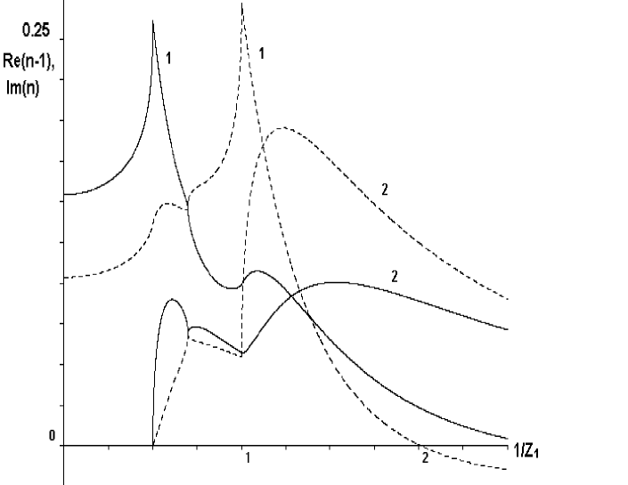
Figure 1: The real (1) and imaginary (2) parts of refractive indices for dichromatic laser wave ($P_{1,1}=1$, $P_{3,2}=1$, $r=0.658$, $z_{2}/z_{1}=2$) as functions of the invariant parameter $z_{1}$. For obtaining absolute quantity the ordinate value is myltiplied by the factor $E_{o}^{2}/\alpha<E^{2}_{1}>$.

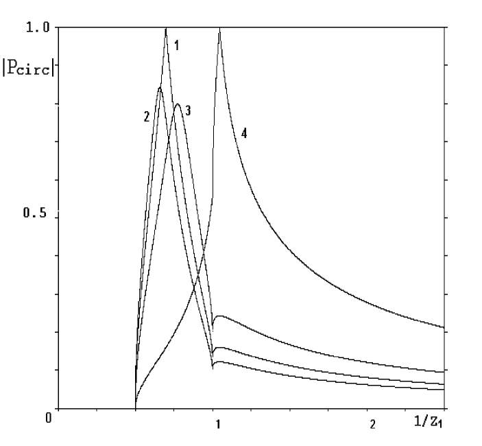
Figure 2: The absolute value of normal waves circular polarizition $|P_{circ}|=|X_{2}|$ as function of the invariant parameter $z_{1}$. The polarization state of laser wave is as in Fig1. The ratios $r$ are equal to 0.658,0.5,1.0 and 4.12 for curves 1-4. The ratio $z_{1}/z_{2}$ is equal to 2.

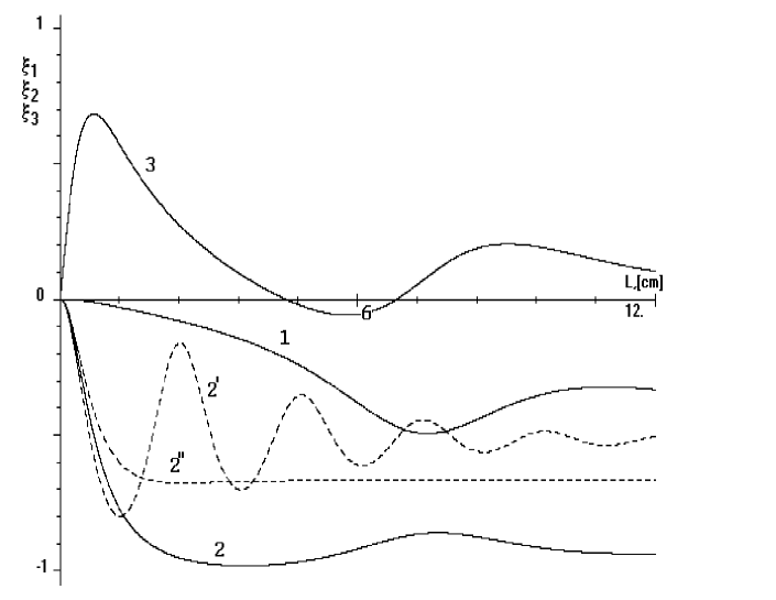
Figure 3: The Stokes parameters of initialy unpolarized $\gamma$-beam as functions of a laser bunch thickness. The polarization state of laser wave is as in Fig.1. The number near each curve corresponds to number i of Stokes parameter $\xi_{i}$. The solid curves correspond to $z_{1}=1.4$. The curves $2^{\prime}$ and $2"$ correspond to $z_{1}=1.2,\,1.6$. $r=0.658$, $z_{1}/z_{2}=2$, $n_{l,1}=5\,10^{25}cm^{-3}$, $E_{l,1}=1eV$.

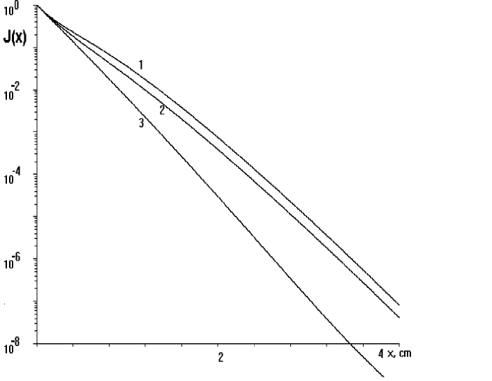
Figure 4: The intensity of $\gamma$-beam as function of the laser bunch thickness. The polarization state of laser wave is as in Fig.1. Curves 1-3 correspond to initial circular polarization $\xi_{2}(0)$ of $\gamma$-beam equals 1, 0 and -1. $r=0.658$, $z_{1}/z_{2}=2$, $n_{l,1}=5\,10^{25}cm^{-3}$, $E_{l,1}=1eV$.

References

• [1] L.D. Landau and E.M.Lifshitz, Electrodynamics of Continuous Media, Pergamon, Oxford (1960).
• [2] V.M. Agranovich and V.L. Ginzburg, Spatial Dispersion in Crystal Optics and the Theory of Excitons, Wiley, New York (1967).
• [3] N.Cabibbo, G. Da Prato, G. De Franceschi, and U. Mosco Phys. Rev. Lett, 1962. V.9 P.435.
• [4] V.N. Baier, V.M.Katkov, and V.M. Strakhovenko, Electromagnetic Processes at High Energies in Oriented Single Crystals [in Russian], Nauka, Novosibirsk, 1989.
• [5] V.A. Maisheev, V.L. Mikhalev, A.M. Frolov, JETP, V.101, p.1376, (1992); Sov.Phys. JETP v.74, p.740, (1992).
• [6] G.L. Kotkin and V.G. Serbo, Preprint hep-ph/9611345 (submitted to Phys. Rev. Lett.)
• [7] B.De Tollis, Il Nuovo Chimento 32, 754 (1964) and 35, 1182 (1965).
• [8] V.B.Berestetskii, E.M. Lifshitz, and L.P. Pitaevskii, Quantum Electrodynamics, Pergamon, Oxford (1982).
• [9] V.A. Maisheev, Preprint IHEP 97-25, Protvino, 1997.
• [10] R.O.Avakian, S.M.Darbinian, K.A.Ispirian, M.K.Ispirian, Nucl.Instr. and Meth., 1986, B 115, P.387.
• [11] A.I. Nikishov, V.I. Ritus JETP v.52, p. 1707 (1967).
• [12] V.G. Baryshevskii and V.V. Tikhomirov, Usp. Fiz. Nauk v.154, p.529, (1989) Sov. Phys. Usp. v. 32, p. 1013 (1989).
• [13] L.D. Landau, and E.M. Lifshitz Statistical Physics , Moscow, Nayka, 1964.
• [14] L.D. Landau, and E.M. Lifshitz, The Classical Theory of Fields, Pergamon, Oxford (1975).
• [15] V.A. Maisheev, V.L. Mikhalev, A.M. Frolov, Preprint IHEP 91-30, Protvino, 1991.
• [16] V.N.Baier, V.M. Katkov, and V.S.Fadin, Radiation from Relativistic Electrons [in Russian], Atomizdat, Moscow, 1973.
• [17] A.M. Frolov, V.A. Maisheev, V.L. Mikhaljov Nucl. Instr. and Meth. 1987 V. A254, P. 549.
• [18] M.H.Salamon and F.W.Stecker. Preprint: astro-ph/9708182
• [19] B.Nodland, J.P.Ralston. Preprint: astro-ph/9704196
Refer to caption