CERN-TH-97-238

FTUV/97-53,IFIC/97-54

hep-ph/9709369

Abstract

We show that the study of CP asymmetries in neutral $B$-meson decays provides a very sensitive probe of flavour-changing neutral currents (FCNC). We introduce two new angles, $\alpha_{SM}$ and $\beta_{SM}$, whose main feature is that they can be readily obtained from the measurement of the CP asymmetries $a_{J/\psi K_{s}}$, $a_{\pi^{+}\pi^{-}}$ and the ratio $R_{u}\equiv|V_{ud}V_{ub}^{*}|/|V_{cd}V_{cb}^{*}|$, providing a quantitative test of the presence of new physics in a model-independent way.

Assuming that new physics is due to the presence of an isosinglet down-type quark, we indicate how to reconstruct the unitarity quadrangles and point out that the measurements of the above asymmetries, within the expected experimental errors, may detect FCNC effects, even for values of $\left|\sum_{i=1}^{3}V_{id}V_{ib}^{*}/(V_{td}V_{tb}^{*})\right|$ at the level of a few times $10^{-2}$.

1 Introduction

The forthcoming experiments at $B$-factories will provide crucial tests of the Standard Model (SM) and its Cabibbo–Kobayashi–Maskawa mechanism (CKM) for flavour mixing and CP violation. The fact that in gauge theories CP violation and flavour mixing arise precisely from their two least known sectors, namely the Yukawa coupling and/or the Higgs sector, enhances the importance of the future experiments on $B$-mesons.

At the moment, there is a considerable amount of data on the CKM mixing matrix, leading to the measurements of $\left|V_{ud}\right|$, $\left|V_{us}\right|$, $\left|V_{ub}\right|$, $\left|V_{cb}\right|$, $\epsilon$, $\epsilon^{\prime}$, $x_{d}$, etc. Since, for three generations, the quark mixing matrix is completely fixed by four parameters, the present experimental data lead in principle to an overdetermination of the CKM matrix. In practice, the situation is more involved, due both to experimental errors and to various hadronic uncertainties in extracting the values of $|V_{ij}|$ from the experimental data. The crucial role played by CP asymmetries in neutral $B$-meson decays such as $B_{d}^{0}\rightarrow J/\psi K_{S}$, $B_{d}^{0}\rightarrow\pi^{+}\pi^{-}$ stems from the fact that, being dominated by one weak decay amplitude, they are free from most of the hadronic uncertainties [1]. In the SM, these CP asymmetries are given by

$$a_{J/\psi K_{S}} = -\frac{\Gamma\left(B^{0}\longrightarrow J/\psi\,K_{s}\right)-\Gamma\left(\overline{B}^{0}\longrightarrow J/\psi\,K_{s}\right)}{\left(\sin(\Delta Mt)\right)\left(\Gamma\left(B^{0}\longrightarrow J/\psi\,K_{s}\right)+\Gamma\left(\overline{B}^{0}\longrightarrow J/\psi\,K_{s}\right)\right)}$$ (1)

$$= \sin 2\beta$$

$$a_{\pi^{+}\pi^{-}} = -\frac{\Gamma\left(B^{0}\longrightarrow\pi^{+}\pi^{-}\right)-\Gamma\left(\overline{B}^{0}\longrightarrow\pi^{+}\pi^{-}\right)}{\left(\sin(\Delta Mt)\right)\left(\Gamma\left(B^{0}\longrightarrow\pi^{+}\pi^{-}\right)+\Gamma\left(\overline{B}^{0}\longrightarrow\pi^{+}\pi^{-}\right)\right)}$$ (2)

$$= \sin 2\alpha$$

where we have adopted the standard definitions of the angles $\alpha$, $\beta$ and $\gamma$ of the unitarity triangle

$$\alpha\equiv\arg\left(-\frac{V_{td}V_{tb}^{*}}{V_{ud}V_{ub}^{*}}\right)$$

$$\beta\equiv\arg\left(-\frac{V_{cd}V_{cb}^{*}}{V_{td}V_{tb}^{*}}\right)$$ (3)

$$\gamma\equiv\arg\left(-\frac{V_{ud}V_{ub}^{*}}{V_{cd}V_{cb}^{*}}\right)$$

In this letter, we will analyse how the presence of new physics can be detected, once the asymmetries $a_{J\psi K_{S}}$, $a_{\pi^{+}\pi^{-}}$ are measured. A good part of our analysis is applicable to a large class of models, although we pay special attention to the detection of flavour-changing neutral currents (FCNC) as well as deviations from $3\times 3$ unitarity of the CKM matrix. In our analysis we will make the following assumptions:

• We will assume that the quark decay amplitudes $\overline{b}\rightarrow\bar{c}c\bar{s}$, $\bar{b}\rightarrow\bar{u}u\bar{d}$, as well as the semileptonic $b$ decays are dominated by the SM tree-level diagrams. This is a reasonable hypothesis, which is satisfied in most of the known extensions of the SM.

• We will allow for the possibility of having new contributions to $B$–$\bar{B}$ mixing as well as deviations from $3\times 3$ unitarity of the CKM matrix.

We will define two new angles, $\alpha_{SM}$, $\beta_{SM}$, which have the interesting feature of being readily obtained from the measured values of $a_{J/\psi K_{S}}$, $a_{\pi^{+}\pi^{-}}$, independently of the presence of new physics. We then indicate how the values of $\alpha_{SM}$, $\beta_{SM}$ can be used to detect in a quantitative way the presence of new physics. This part of the analysis uses as experimental input only the values of $a_{J/\psi K_{S}}$, $a_{\pi^{+}\pi^{-}}$ and the ratio $R_{u}\equiv|V_{ud}V_{ub}^{*}|/|V_{cd}V_{cb}^{*}|$. Using then the experimental value of the $B^{0}$–$\overline{B}^{0}$ mixing parameter $x_{d}$, we will show how deviations of $3\times 3$ unitarity can be established by full reconstruction of a unitarity quadrangle in the context of models extended with one isosinglet vector-like quark of the down type (VLdQ) [2]. We will show that CP asymmetries in B decays provide a very sensitive probe on deviations from $3\times 3$ unitarity, measured by the parameter $Z_{bd}$, defined by

$$Z_{bd}=V_{ud}V_{ub}^{*}+V_{cd}V_{cb}^{*}+V_{td}V_{tb}^{*}.$$ (4)

We will give the minimum value of $Z_{bd}$ that can be detected at $B$-factories, taking into account the expected experimental errors.

2 Model-independent analysis

It is clear from Eq. (1) that the angles $\alpha$, $\beta$, $\gamma$ satisfy, by definition, the relation $\alpha+\beta+\gamma=\arg(-1)=\pi$. This relation obviously holds in any model, and one can write $\gamma=\pi-(\alpha+\beta)$. We will allow for the possibility of having new physics in the $B$–$\overline{B}$ mixing, which we will parametrize as

$$M_{12}=M_{12}^{(SM)}\Delta_{bd}^{*}$$ (5)

where $M_{12}^{(SM)}$ is the standard box contribution and $\Delta_{bd}$ is a complex number that parametrizes the new physics. The CP asymmetries are then given by

$$\begin{array}[]{l}a_{J/\psi K_{s}}=\sin\left(2\beta-\arg\Delta_{bd}\right)\\ a_{\pi^{+}\pi^{-}}=\sin\left(2\alpha+\arg\Delta_{bd}\right).\end{array}$$ (6)

From this equation it is clear that $\alpha+\beta$ can be extracted in a model-independent way, and one has

$$\pi-\gamma=\left(\alpha+\beta\right)=\frac{1}{2}\left[\arcsin(a_{J/\Psi,K_{s}})+\arcsin(a_{\pi^{+}\pi^{-}})\right].$$ (7)

At this stage, it is useful to introduce the two angles $\alpha_{SM}$ and $\beta_{SM}$, defined by (see Fig. 1)

$$\alpha_{SM}=\arg\left[\frac{\left(V_{ud}V_{ub}^{*}+V_{cd}V_{cb}^{*}\right)}{V_{ud}V_{ub}^{*}}\right]$$

$$\beta_{SM}=\arg\left[\frac{V_{cd}V_{cb}^{*}}{\left(V_{ud}V_{ub}^{*}+V_{cd}V_{cb}^{*}\right)}\right].$$ (8)

In models that respect 3$\times$ 3 unitarity, and in particular where $Z_{bd}=0$, one obviously has $\alpha=\alpha_{SM}$ and $\beta=\beta_{SM}$, but this will not be the case in models where $Z_{bd}\neq 0$. The advantage of the new angles $\alpha_{SM}$, $\beta_{SM}$ results from the fact that they can be readily obtained from the measurements of $a_{J/\psi K_{S}}$, $a_{\pi^{+}\pi^{-}}$ together with the ratio $R_{u}$. Indeed from Eq. (8), one has,

$$\alpha_{SM}=\arctan\left[\frac{\sin\gamma}{R_{u}+\cos(\pi-\gamma)}\right]$$

$$\beta_{SM}=\arctan\left[\frac{R_{u}\sin\gamma}{1+R_{u}\cos(\pi-\gamma)}\right],$$ (9)

where $R_{u}=|V_{ud}V_{ub}^{*}|/|V_{cd}V_{cb}^{*}|$ and $\gamma$ is obtained from Eq. (7). It should be emphasized that even if new physics is present in $B$–$\overline{B}$ mixing and/or there are deviations from unitarity, $\alpha_{SM}$, $\beta_{SM}$ are obtained in a model-independent way from Eq. (2).

We are specially interested in detecting any deviation of the measured values of the asymmetries $a_{J/\psi K_{s}}$, $a_{\pi^{+}\pi^{-}}$ from the predictions of the standard model. These deviations can be defined as

$$\Delta_{J/\psi K_{S}}\equiv(a_{J/\psi K_{S}})_{measured}-(a_{J/\psi K_{S}})_{SM}$$

$$\Delta_{\pi^{+}\pi^{-}}\equiv(a_{\pi^{+}\pi^{-}})_{measured}-(a_{\pi^{+}\pi^{-}})_{SM},$$ (10)

where $(a_{J/\psi K_{S}})_{SM}$, $(a_{\pi^{+}\pi^{-}})_{SM}$ are the predicted values of the asymmetries in the SM, namely:

$$\begin{array}[]{l}(a_{J/\Psi,K_{s}})_{SM}=\sin 2\beta_{SM}\\ (a_{\pi^{+}\pi^{-}})_{SM}=\sin 2\alpha_{SM},\end{array}$$ (11)

Since $\alpha_{SM}$, $\beta_{SM}$ can be evaluated from Eq. (2), one can obtain $\Delta_{J/\psi K_{S}}$, $\Delta_{\pi^{+}\pi^{-}}$ having as experimental input only the experimental values of $a_{J/\psi K_{S}}$, $a_{\pi^{+}\pi^{-}}$. Non-vanishing values of $\Delta_{J/\psi K_{S}}$, $\Delta_{\pi^{+}\pi^{-}}$ indicate in a quantitative way the presence of new physics.

For the analysis that follows, it is useful to define $\delta\equiv\beta-\beta_{SM}$, which implies $\alpha=\alpha_{SM}-\delta$ (see Fig. 1). It is clear that the combination $2\delta-\arg\Delta_{bd}$ can be readily evaluated from the previous analysis and one has

$$(2\delta-\arg\Delta_{bd})=\arcsin(a_{J/\psi K_{S}})-2\beta_{SM}.$$ (12)

Notice that a deviation from zero in Eq. (12) would translate in a corresponding non-zero value in Eq. (10). Therefore $2\delta-\arg\Delta_{bd}$ can also be used as a measure of the presence of new physics in CP asymmetries.

An additional piece of information that can be extracted from the previous analysis is the side opposite to the angle $\gamma$ in the triangle with angles $(\alpha_{SM},\beta_{SM},\gamma)$:

$$L_{uc}\equiv|V_{ud}V_{ub}^{*}+V_{cd}V_{cb}^{*}|.$$ (13)

With the experimental knowledge of $|V_{ud}V_{ub}^{*}|$, $|V_{cd}V_{cb}^{*}|$ as well as the value of $\gamma$ extracted from Eq. (7), one readily obtains $L_{uc}$.

So far, we have not used in our analysis the experimental value of the $B^{0}$–$\overline{B}^{0}$ mixing parameter $x_{d}$. In the SM, $L_{uc}=|V_{td}V_{tb}^{*}|$; therefore, a second test of the SM comes from the comparison of $|L_{uc}|$ with the value of $|V_{td}V_{tb}^{*}|$ extracted from the value of $x_{d}$, in the framework of the SM. If the equation

$$\begin{array}[]{l}x_{d}=C_{d}L_{uc}^{2}\\ \\ C_{d}=\frac{G_{F}^{2}\eta_{B}M_{B_{d}}}{6\pi^{2}\Gamma_{B_{d}}}(B_{B_{d}}F_{B_{d}}^{2})M_{W}^{2}\mid\overline{E}(x_{t}\mid)\end{array}$$

is not fulfilled, this will be a clear indication of the presence of new physics beyond the SM. We have used standard notation for the parameters entering $C_{d}$, and their experimental values can be found in Ref. [3]. In a general model, with a new contribution to $B_{d}$–$\overline{B}_{d}$ mixing, one has

$$x_{d}=C_{d}\left|\Delta_{bd}\right|\left|V_{td}V_{tb}^{*}\right|^{2}.$$ (14)

At this stage, it is worth recalling all the information we have about the unitarity quadrangle. From $\left|V_{ud}V_{ub}^{*}\right|$, $\left|V_{cd}V_{cb}^{*}\right|$, $a_{J/\Psi,K_{s}}$ and $a_{\pi^{+}\pi^{-}}$ we have fully reconstructed the $(\alpha_{SM},\beta_{SM},\gamma)$-triangle. The parameter $2\delta-\arg\Delta_{bd}$ is also obtained from Eq. (12), while $x_{d}$ gives us the value of $|\Delta_{bd}||V_{td}V_{tb}^{*}|^{2}$. From Fig. 1 it is clear that, in order to obtain the full quadrangle, we need to reconstruct the triangle with sides $L_{uc}$, $|Z_{bd}|$ and $|V_{td}V_{tb}^{*}|$. Next we will indicate how the full quadrangle can be reconstructed in the specific case where the new contributions to $B_{d}$–$\overline{B}_{d}$ mixing are due to FCNC arising in the context of a model where the SM is extended, through the addition of an isosinglet VLdQ. In this case $\Delta_{bd}$ is given by

$$\Delta_{bd}=1+are^{i\phi}-br^{2}e^{2i\phi}$$

$$re^{i\phi}=\frac{Z_{bd}}{V_{td}V_{tb}^{*}}$$

$$a=\frac{4\overline{C}(x_{t})}{\overline{E}(x_{t})}$$ (15)

$$b=\frac{4\pi\sin^{2}\theta_{W}}{\alpha\overline{E}(x_{t})},$$

where $\overline{E}(x_{t})$ and $\overline{C}(x_{t})$ are the well-known Inami and Lim functions [4]:

$$\overline{E}(x)=\frac{-4x+11x^{2}-x^{3}}{4(1-x)^{2}}+\frac{3x^{3}\ln x}{2(1-x)^{3}}$$

$$\overline{C}(x_{t})=\frac{x}{4}\left[\frac{4-x}{1-x}+\frac{3x\ln x}{(1-x)^{2}}\right]$$ (16)

and $x_{t}=\left(m_{t}/M_{W}\right)^{2}$. The last term in $\Delta_{bd}$, with an $r^{2}$ dependence, arises from the well-known $Z$-flavour-changing tree-graph contribution. The second term, with a linear dependence in $r$, comes from a one-loop $Z$-vertex correction, as recently pointed out in Ref. [5]. From Eq. (2) and Fig. 1, it is evident that we are led, from the knowledge of $|\Delta_{bd}||V_{td}V_{tb}^{*}|^{2}$, $2\delta-\arg\Delta_{bd}$ and $L_{uc}$, to three equations with three unknowns $r$, $\phi$, $|V_{td}V_{tb}^{*}|$. Note that these last three variables completely fix the upper triangle, therefore $\delta$ and $L_{uc}$ can be written in terms of $r$, $\phi$ and $|V_{td}V_{tb}^{*}|$. We can thus reconstruct the triangle of sides $L_{uc}$, $|V_{td}V_{tb}^{*}|$, $|Z_{bd}|$, completing in this way the reconstruction of the unitarity quadrangle.

It should be pointed out that discrete ambiguities may occur in the extraction of the value of the various angles from the knowledge of the asymmetries. A detailed discussion of how to overcome these ambiguities through additional measurements can be found in Ref. [6]. Throughout this paper, we will assume that these ambiguities can be solved by using additional information. We also assume that in the case of $\pi^{+}\pi^{-}$, possible complications, which may arise due to penguin contributions to the decay amplitudes, can be dealt with by using the analysis proposed in Ref. [7].

3 Quadrangle reconstructions

In VLdQ models one can choose, without loss of generality, a weak basis where the up quark mass matrix is diagonal. The mixing is then described by the 4$\times$4 unitary matrix $V$, which diagonalizes the down quark mass matrix. $V_{CKM}$ is the upper 3$\times$4 submatrix of $V$ and the elements of the fourth row fix the FCNC couplings of the $Z$-boson, $Z_{qq^{\prime}}=-V_{4q^{\prime}}V_{4q}^{*}$. The actual experimental bounds on $V$ coming from tree-level processes are [3]:

$$\left[\begin{array}[]{llll}0.973-0.975&0.2187-0.223&0.0024-0.0040&-\\ 0.208-0.240&0.83-1&0.037-0.043&-\\ -&-&-&-\\ -&-&-&-\end{array}\right]$$ (17)

From rare decays such as $K^{+}\rightarrow\pi^{+}\nu\overline{\nu}$ and $b\rightarrow Xl^{+}l^{-}$ one obtains [8]:

$$\begin{array}[]{l}\left|Z_{sd}\right|\leq 4.8\times 10^{-5}\\ \left|Z_{bd}\right|,\left|Z_{bs}\right|\leq 1.9\times 10^{-3}\end{array}$$ (18)

and finally, from $x_{d}$:

$$6.9\times 10^{-3}\leq\left|V_{td}V_{tb}^{*}\right|\left|\Delta_{bd}\right|^{1/2}\leq 11.3\times 10^{-3}$$ (19)

where the hadronic uncertainties have been included.

The purpose of our analysis is to show through specific examples how with the knowledge of the experimental values of the CP asymmetries $a_{J/\psi K_{S}}$, $a_{\pi^{+}\pi^{-}}$, and with the experimental errors expected in $B$-factories, one may be able to detect new physics beyond the SM. With the assumption that new physics arises from the VLdQ model, we will show that one can fully reconstruct the unitarity quadrangles. In our analysis we have adopted the following strategy. We have made a scan of $4\times 4$ unitary matrices, using one of the standard parametrizations [9], which on the one hand satisfy all the constraints in Eqs. (17), (18), (19) and, on the other hand, lead to predictions to $(a_{J/\psi K_{S}},a_{\pi^{+}\pi^{-}})$ that differ significantly from the predictions of the SM. We have classified the solutions in two groups with the following features.

• Case I. Relatively large value of the parameter $r$ (e.g. $r\approx 0.2$), leading to a large value of $\arg\Delta_{bd}$, while the deviations from $3\times 3$ unitarity, entering in the asymmetries through $\delta$, remain relatively small. Then the effects of new physics in the asymmetries are clearly dominated by the mixing.

• Case II. Small values of $r$ (e.g. $r\approx 0.05$) and new physics both in the mixing, $\arg\Delta_{bd}$, and in the quadrangle $\delta$.

For definiteness, we will consider two examples of unitary matrices belonging to each one of the cases. We will then consider two realistic situations where one knows $(a_{J/\psi K_{S}},a_{\pi^{+}\pi^{-}})$, $\left|V_{ud}V_{ub}^{*}\right|$, $\left|V_{cd}V_{cb}^{*}\right|$, $x_{d}$, only within some experimental errors. The central values of $a_{J/\psi K_{S}}$, $a_{\pi^{+}\pi^{-}}$ are chosen as the values implied by the above-mentioned unitary matrices, belonging to cases I and II. We will show that in each of these two cases, one would be able to establish the existence of new physics (i.e. $r\neq 0$) and find the allowed ranges of $r$ and $\phi$.

Let us consider the following explicit examples:

• Case I: $r\simeq 0.185$, new physics in the mixing

$$\left|V\right|=\left[\begin{array}[]{cccc}0.\,97496&0.\,2223&3.\,9999\times 10^{-3}&0.00\,492\\ 0.\,22229&0.\,97423&3.\,7998\times 10^{-2}&4.\,9666\times 10^{-3}\\ 4.\,8288\times 10^{-3}&3.\,7284\times 10^{-2}&0.\,97745&0.\,20782\\ 4.\,1991\times 10^{-3}&8.\,8125\times 10^{-3}&0.\,2077&0.\,97814\end{array}\right]$$ (20)

$$\arg(V)=\left[\begin{array}[]{cccc}0&0&-0.\,41888&2.\,0944\\ -3.\,1414&-1.\,1839\times 10^{-5}&1.\,9116\times 10^{-6}&1.\,6755\\ 2.\,6719&4.\,1595\times 10^{-2}&3.\,1416&0\\ -2.\,4556&-0.\,68252&-3.\,1407&3.\,1416\end{array}\right]$$ (21)

The corresponding unitarity quadrangle is represented in Fig. 2.

In this case, one has a relatively large value of $r$( $r=0.\,18478$), and there is new physics in the mixing corresponding to $\arg(\Delta_{bd})=2.\,0659$ versus $\delta\equiv\beta-\beta_{SM}=0.156$. There are clearly detectable effects in $a_{J/\psi K_{S}}$ and $a_{\pi^{+}\pi^{-}}$, as can be seen by comparing to the values of $\sin 2\beta_{SM}$ and $\sin 2\alpha_{SM}$:

$$a_{J/\psi K_{S}}=-0.\,90274 a_{\pi^{+}\pi^{-}}=0.\,28481$$ (22)

$$\sin(2\beta_{SM})=0.\,58736 \sin(2\alpha_{SM})=-0.\,99442$$

• Case II: $r\simeq 5\times 10^{-2}$ , new physics in the quadrangle and the mixing

  $$\left|V\right|=\left[\begin{array}[]{cccc}0.\,97496&0.\,2223&3.\,9999\times 10^{-3}&0.00\,492\\ 0.\,22197&0.\,97422&3.\,9989\times 10^{-2}&4.\,9666\times 10^{-3}\\ 0.0\,1316&3.\,7863\times 10^{-2}&0.\,9773&0.\,20801\\ 3.\,1224\times 10^{-3}&6.\,8898\times 10^{-3}&0.\,20799&0.\,9781\end{array}\right]$$ (23)

$$\arg(V)=\left[\begin{array}[]{cccc}0&0&-2.\,9322&-2.\,0944\\ -3.\,1413&-1.\,2891\times 10^{-5}&2.\,4309\times 10^{-6}&-0.\,83776\\ 3.\,0284&2.\,9735\times 10^{-2}&3.\,1416&3.\,1416\\ 1.\,7074&2.\,4479&6.\,2532\times 10^{-4}&3.\,1416\end{array}\right]$$ (24)

The corresponding unitarity quadrangle is represented in Fig. 3.

In this case one has a rather small value of $r$ ( $r=5.\,0494\times 10^{-2}$), while $\arg(\Delta_{bd})=-6.\,8996\times 10^{-2}$ and $\delta=4.\,9506\times 10^{-2}$. There are also detectable effects of new physics in the CP asymmetries, since one has:

$$a_{J/\psi K_{S}}=0.\,29147 a_{\pi^{+}\pi^{-}}=0.\,1233$$ (25)

$$\sin(2\beta_{SM})=0.\,12741 \sin(2\alpha_{SM})=0.\,2875$$

These two examples are the starting point of our analysis of realistic situations where the input data are only known within some experimental errors. At this stage it is worth indicating how the unitarity quadrangle can be reconstructed, taking as input data $a_{J/\psi K_{S}}$, $a_{\pi^{+}\pi^{-}}$, $\left|V_{ud}V_{ub}^{*}\right|$, $\left|V_{cd}V_{cb}^{*}\right|$ and $x_{d}$. We will use the following relations:

$$L_{uc}=\left|V_{cd}V_{cb}^{*}\right|\sqrt{1+R_{u}^{2}\mp\sqrt{2}R_{u}\sqrt{1+\left[\pm\sqrt{\left(1-a_{J/\psi K_{S}}^{2}\right)\left(1-a_{\pi^{+}\pi^{-}}^{2}\right)}-a_{J/\psi K_{S}}a_{\pi^{+}\pi^{-}}\right]}}$$ (26)

$$2\delta-\arg(\Delta_{bd})=2\arg\left\{1+R_{u}e^{-\frac{i}{2}\left[\arcsin\left(a_{\pi^{+}\pi^{-}}\right)+\arcsin\left(a_{J/\psi K_{S}}\right)\right]}\right\}+\arcsin\left(a_{J/\psi K_{S}}\right)$$ (27)

$$e^{i\left(2\delta-\arg\left(\Delta_{bd}\right)\right)}=\frac{(1-re^{i\phi)^{2}}\left(1+are^{i\phi}-br^{2}e^{2i\phi}\right)^{*}}{\left|1-re^{i\phi}\right|^{2}\left|1+are^{i\phi}-br^{2}e^{2i\phi}\right|}$$ (28)

$$\frac{x_{d}}{C_{d}L_{uc}^{2}}=\frac{\left|1+are^{i\phi}-br^{2}e^{2i\phi}\right|}{\left|1-re^{i\phi}\right|^{2}},$$ (29)

where we have expressed $|V_{td}V_{tb}^{*}|$ in terms of $r$, $\phi$ and $L_{uc}$ using,

$$|V_{td}V_{tb}^{*}|=\frac{L_{uc}}{|1-re^{i\phi}|}.$$ (30)

It is clear that using Eqs. (26), (27) and the measured values of $a_{J/\psi K_{S}}$, $a_{\pi^{+}\pi^{-}}$, $\left|V_{cd}V_{cb}^{*}\right|$ and $\left|V_{ud}V_{ub}^{*}\right|$ one can obtain $L_{uc}$ and $2\delta-\arg(\Delta_{bd})$. One can then use Eqs. (28), (29) and the measured value of $x_{d}$ to obtain $r$ and $\phi$. Therefore we can fully reconstruct the quadrangle and obtain the important quantity $re^{i\phi}=\frac{Z_{bd}}{V_{td}V_{tb}^{*}}$, which is a measure of the deviation of 3$\times$ 3 unitarity in the framework of the VLdQ model.

Next, we will assume that the measurement of $a_{J/\psi K_{S}}$, $a_{\pi^{+}\pi^{-}}$ gives the central values corresponding to Case I, with the following experimental errors:

$$a_{J/\psi K_{S}}=-0.90\pm 0.08$$

$$a_{\pi^{+}\pi^{-}}=0.28\pm 0.08$$ (31)

where the errors probably are pessimistic for $a_{J/\psi K_{S}}$ and optimistic for $a_{\pi^{+}\pi^{-}}$ in the case of a $B$-factory. From these “experimental” data, together with $\left|V_{cd}V_{cb}^{*}\right|$, $\left|V_{ud}V_{ub}^{*}\right|$ (including of course their actual errors) and the experimental value of $x_{d}$ (with the hadronic uncertainties included in $C_{d}$) we get in this case

$$\begin{array}[]{l}\cos\left(2\delta-\arg(\Delta_{bd})\right)=0.06\pm 0.31\\ \sin\left(2\delta-\arg(\Delta_{bd})\right)=-0.998\pm 0.017\\ 0.90\leq\frac{x_{d}}{C_{d}\left|L_{uc}\right|^{2}}\leq 5.13.\end{array}$$ (32)

The values given in Eq. (32) can be plugged in Eqs. (28) and (29) in order to obtain $re^{i\phi}=x+iy$. Note that the value of the angle $2\delta-\arg(\Delta_{bd})$ would be quite far from its value in the SM, where it vanishes. Therefore, in this case the detection of new physics would be unambiguously established. Note that in the derivation of the result of Eq. (32), we have assumed that the discrete ambiguities in Eqs. (26), (27) can be solved by using additional information, as pointed out in Ref. [6]. The plot of Eqs. (28) and (29), with the allowed bands (Eq. (32)) is given in Fig. 4.

The region between the external circle and the two internal ones is allowed by the $x_{d}$ ranges. The overlap of this sector with the allowed regions for $\sin\left(2\delta-\arg(\Delta_{bd})\right)$ and $\cos\left(2\delta-\arg(\Delta_{bd})\right)$ is the solution region we get for $re^{i\phi}=x+iy$ (darker area). The input values in Case I are $x=-0.075$ and $y=-0.17$, so the region in the third quadrant of Fig. 4 corresponds to the inputs of Case I. To be sure that the other solution in Fig. 4 is physical, it would be necessary to perform a very fine scanning of the parameter space of the mixing matrix. We will not address this question in this paper and we will concentrate on the reconstructed solution that corresponds to the input parameters. Therefore we conclude that roughly speaking we get a value of $r$ between $0.1$ and $0.2$, never compatible with the standard model, even if we enlarge the error bars by several standard deviations. The two seagull-shaped regions correspond to the $\cos\left(2\delta-\arg\left(\Delta_{bd}\right)\right)$ curves, the $\sin\left(2\delta-\arg\left(\Delta_{bd}\right)\right)$ curve serves to eliminate the wings in the second and fourth quadrants. It is evident from equation (28) that the curves $\cos\left(2\delta-\arg\left(\Delta_{bd}\right)\right)=cst$ will pass through the points $\Delta_{bd}=0$ that correspond to the “centre” of the small circles

$$x = \frac{a}{2b}=9.\,92\times 10^{-3}$$

$$y = \pm\sqrt{-\frac{1}{b}\left(1+\frac{a^{2}}{2b}\right)}=\pm 7.\,66\times 10^{-2}$$ (33)

$$r = 0.0\,77$$

It is precisely this value of $r$ that fixes the scale of $r$ lower bound in Fig. 4. The upper bound of $r$ is fixed by the upper bound of $\frac{x_{d}}{C_{d}\left|L_{uc}\right|^{2}}$ (the external circle); therefore the larger $L_{uc}$ can be, the better upper bound for $r$. In this case, as it is evident from Fig. 2, $L_{uc}=\left(6.3\pm 1.1\right)\times 10^{-3}$ is small. From this simple consideration, we can expect to obtain in Case II a much better upper bound for $r$, since from Fig. 3 one can see that $L_{uc}$ has a larger value.

Finally, let us consider Case II, where we assume the following values for $a_{J/\psi K_{S}}$, $a_{\pi^{+}\pi^{-}}$:

$$a_{J/\psi K_{S}}=0.29\pm 0.08, a_{\pi^{+}\pi^{-}}=0.12\pm 0.08,$$ (34)

which lead to

$$\begin{array}[]{l}\cos\left(2\delta-\arg(\Delta_{bd})\right)=0.98\pm 0.01\\ \sin\left(2\delta-\arg(\Delta_{bd})\right)=0.19\pm 0.07\\ 0.274\leq\frac{x_{d}}{C_{d}\left|L_{uc}\right|^{2}}\leq 1.10.\end{array}$$ (35)

Several comments are in order. The angle $2\delta-\arg(\Delta_{bd})$ is three standard deviations away from its standard model value of 0. This is to be expected, since $a_{J/\psi K_{S}}$ is also three standard deviations away from $\sin\left(2\beta_{SM}\right)$. The upper bound of $\frac{x_{d}}{C_{d}L_{uc}^{2}}$ is much smaller than in Case I as we have anticipated above. As we will see these facts completely change the origin of the scales of the bounds in $r$ . The analog of Fig. 4 for the Case II is plotted in Fig. 5.

The input parameters in this second case are $x=0.012$ and $y=-0.049$, therefore the solution corresponds to the dark area in the fourth quadrant. The solutions have changed quadrants because $\sin\left(2\delta\right.-$ $\left.\arg(\Delta_{bd})\right)$ has changed sign. Clearly in this case the upper bound on r ($r\ \hbox to0.0pt{\raise 2.0pt\hbox{$<$}\hss}{\lower 2.0pt\hbox{$\sim$}}\ 0.065$) is fixed by the centre of the down small circle defined by $\frac{x_{d}}{C_{d}\left|L_{uc}\right|^{2}}=0.274$. A reduction of the hadronic uncertainties in $C_{d}$ would lead to an increase of the radius of this small circle, thus reducing the upper bound on $r$. The lower bound on $r$ ($r\ \hbox to0.0pt{\raise 2.0pt\hbox{$>$}\hss}{\lower 2.0pt\hbox{$\sim$}}\ 0.04$) has to be taken with some caution, since it is compatible with zero at less than three standard deviations.

At any rate, it is clear from the above analysis that the study of CP asymmetries at $B$-factories provides the possibility of putting stringent bounds on $\left|\frac{Z_{bd}}{V_{td}V_{tb}^{*}}\right|$, of the order of 0.065 or even smaller. Therefore $B$-factories are quite competitive with respect to other experiments looking directly for FCNC in $b\rightarrow d$ transitions.

4 Conclusions

We have pointed out that the study of CP asymmetries in B decays provides an excellent tool for testing the SM and probing for new physics. In the framework of the SM, the CP asymmetries $a_{J/\psi K_{s}}$, $a_{\pi^{+}\pi^{-}}$ measure the angles of the unitarity triangle. If one wants to allow for the possiblity of having new physics in the $B$–$\overline{B}$ mixing and/or deviations of 3$\times$3 unitarity of the CKM matrix, the analysis becomes more involved. We found it useful to introduce two new angles, $\alpha_{SM}$ and $\beta_{SM}$, whose important feature is the fact that they are readily obtained from the measurement of $a_{J/\psi K_{s}}$ , $a_{\pi^{+}\pi^{-}}$ and the ratio $R_{u}$, even in the presence of new physics. The knowledge of $\alpha_{SM}$ and $\beta_{SM}$ enables us to ckdetect in a quantitative way deviations from the SM predictions for the CP asymmetries.

Assuming that the new physics arises from deviations from 3$\times$3 unitarity, which in turn leads to FCNC, we show how to reconstruct the unitarity quadrangle from input data. A study of specific examples shows that even taking into account the expected errors in the experimental values of $a_{J/\psi K_{s}}$, $a_{\pi^{+}\pi^{-}}$, it may be possible to detect the presence of the FCNC coupling $Z_{bd}$, even for a rather small value of the ratio $\left|\frac{Z_{bd}}{V_{td}V_{tb}^{*}}\right|$.

ACKNOWLEDGEMENTS

We would like to thank J. Bernabéu and F. del Aguila for useful comments and discussions. G.B. acknowledges the Spanish Ministry of Foreign Affairs for a MUTIS fellowship, and O.V. acknowledges the Generalitat Valenciana for a research fellowship. G.C. Branco is grateful to the CERN Theory Division for kind hospitality, and thanks Michael Gronau for various conversations. This work is partially supported by CICYT under grant AEN-96-1718 and IVEI under grant 038/96.

Figure 1: The unitarity quadrangle, with angles $\alpha$, $\beta$, $\gamma$, $\alpha_{SM}$, $\beta_{SM}$. In the SM limit one has $\alpha_{SM}=\alpha$, $\beta_{SM}=\beta$.

Figure 2: The unitarity quadrangle for case I, corresponding to a relatively large contribution of new physics in the mixing, $r=0.185$

Figure 3: The unitarity quadrangle for case II, corresponding to $r=5\cdot 10^{-2}$

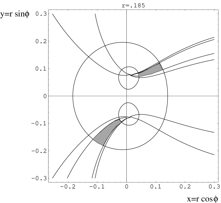
Figure 4: Reconstruction of $(r,\phi)$ from the measurement of the asymmetries in Case I

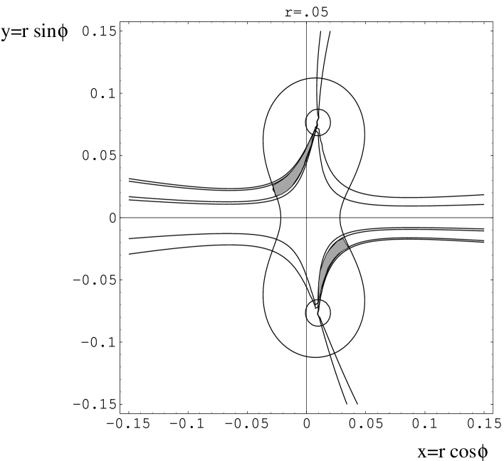
Figure 5: Reconstruction of $(r,\phi)$ from the measurement of the asymmetries in Case II

References

- [1] For the general formalism of CP asymmetries in neutral decays, see for instance, Y.Nir and H.Quinn, Ann. Rev. Nucl. Part. Sci. 42 (1992) 211.
-
[2]
F.del Aguila and J.Cortés, Phys. Lett. B156 (1985) 243,
G.C.Branco and L.Lavoura, Nucl. Phys. B278 (1986) 738,
F.del Aguila, M.K.Chase and J.Cortés, Nucl. Phys. B271 (1986) 61,
Y.Nir and D.Silverman, Phys. Rev. D42 (1990) 1477,
D.Silverman, Phys. Rev. D45 (1992) 1800,
G.C.Branco, T.Morozumi, P.A.Parada and M.N.Rebelo, Phys. Rev. D48 (1993), 1167.
W-S.Choong and D.Silverman, Phys. Rev. D49 (1994) 2322,
V.Barger, M.S.Berger and R.J.N.Phillips, Phys. Rev. D52 (1995) 1663,
D.Silverman,Int. Jour. Mod. Phys. A11 (1996) 2253,
M.Gronau and D.London, Phys. Rev. D55 (1997) 2845,
F.del Aguila, J.A.Aguilar-Saavedra and G.C.Branco, UG-FT 69/97, hep.ph/9703410, March 1997 - [3] A.J.Buras and R.Fleischer, Quark mixing, CP violation and rare decays after the top quark discovery , to appear in Heavy Flavours II, eds. A.J.Buras and M.Lindner, Advanced Series on Directions in High Energy Physics, World Scientific (1997).
- [4] C.S. Lim and T. Inami, Prog. Theor. Phys. 65 (1981) 297.
- [5] G.Barenboim and F.J.Botella, FTUV/97-53, IFIC/9754, hep-ph/9708209, to appear in Phys. Lett. B
-
[6]
Y.Grossman and H.R.Quinn, SLAC-PUB-7454, hep-ph/9705356,
Y.Grossman Y. Nir and M.P.Worah, hep-ph/9704287 -
[7]
M. Gronau and D. London, Phys. Rev. Lett. 65 (1990) 3381,
M. Gronau and J.L. Rosner Phys. Rev. Lett. 76 (1996) 1200. -
[8]
C.Albajar et al., UA1 Collaboration, Phys. Lett. B262 (1991) 163,
Y.Grossman, Z.Ligeti and E.Nardi, Nucl. Phys. B465 (1996) 369, (E) Nucl. Phys. B480 (1996) 753,
ALEPH Collaboration, Report no. PA10-019, presented at the 18th International Conference on High Energy Physics, Warsaw, Poland (1996),
D0Collaboartion, Report no. FERMILAB-CONF-96/253-E, presented at the 28th International Conference on High Energy Physics, Warsaw, Poland (1996),
Y.Grossman, Y.Nir and R.Rattazzi, CP violation beyond the Standard Model, to appear in Heavy Flavours II, eds. A.J.Buras and M.Lindner, Advanced Series on Directions in High Energy Physics, World Scientific (1997). - [9] F.J.Botella and L.L.Chau, Phys. Lett. 168B (1986) 97.